A Bayesian nonparametric mixture model for selecting genes and gene subnetworks

Abstract

It is very challenging to select informative features from tens of thousands of measured features in high-throughput data analysis. Recently, several parametric/regression models have been developed utilizing the gene network information to select genes or pathways strongly associated with a clinical/biological outcome. Alternatively, in this paper, we propose a nonparametric Bayesian model for gene selection incorporating network information. In addition to identifying genes that have a strong association with a clinical outcome, our model can select genes with particular expressional behavior, in which case the regression models are not directly applicable. We show that our proposed model is equivalent to an infinity mixture model for which we develop a posterior computation algorithm based on Markov chain Monte Carlo (MCMC) methods. We also propose two fast computing algorithms that approximate the posterior simulation with good accuracy but relatively low computational cost. We illustrate our methods on simulation studies and the analysis of Spellman yeast cell cycle microarray data.

, and t1Equally contributed. t2Supported in part by the National Center for Advancing Translational Sciences of the National Institutes of Health under Award Number UL1TR000454. t3Supported in part by the National Institutes of Health grants P20 HL113451 and U19 AI090023.

1 Introduction

In high-throughput data analysis, selecting informative features from tens of thousands of measured features is a difficult problem. Incorporating pathway or network information into the analysis has been a promising approach. Generally the setup of the problem contains two pieces of information. The first is the measurements of the features in multiple samples, typically with a clinical outcome associated with each sample. The second piece of information is a network depicting the biological relationship between the features, which is based on existing biological knowledge. The network could contain information such as protein interaction, transcriptional regulation, enzymatic reaction and signal transduction, etc. [Cerami et al. (2011)].

Some methods are developed using the available network topology for high-throughput data analysis. These methods incorporate the gene-pathway relationships or gene network information into a parametric/regression model. The primary goal is to identify either the important pathways or the genes that are strongly associated with clinical outcomes of interest. For example, there are a series of works [Wei and Li (2007, 2008); Wei and Pan (2010)] that model the gene network using a Discrete or Gaussian Markov random field (DMRF or GMRF). Li and Li (2008) and Pan, Xie and Shen (2010) used the gene network to build penalties in a regression model for gene pathway selection. Ma et al. (2010) incorporated the gene co-expression network in identification of caner prognosis markers using a survival model. Li and Zhang (2010) and Stingo et al. (2011) developed Bayesian linear regression models using MRF priors or Ising priors that capture the dependent structure of transcription factors or the gene network/pathway. Recently, Jacob, Neuvial and Dudoit (2012) proposed a powerful graph-structured two-sample test to detect differentially expressed genes.

Although regression models are widely used for the selection of the gene subnetwork that is associated with an outcome variable, in some situations the question of interest is to study the expressional behavior of genes, for example, periodicity, without an outcome variable. In other situations, the experimental design is more complex than simple case-control. For example, some gene expression studies involve longitudinal/functional measurements for which the parametric models [Leng and Müller (2006); Zhou et al. (2010); Breeze et al. (2011)] or the multivariate testing procedure [Jacob, Neuvial and Dudoit (2012)] may not be applicable without a major modification. A straightforward approach to this problem is to perform large-scale simultaneous hypothesis testing on gene behavior. A set of genes can be selected based on the testing statistics or $p$-values, where a correct choice of a null distribution for those correlated testing statistics [Efron (2004, 2010)] should be used. However, this approach ignores the gene network information that is useful to identify the subnetwork of genes with the particular expressional behavior. Due to the diverse behavior of neighboring genes on the network, it is generally believed that genes in close proximity on a network are likely to have joint effects on biological/medical outcomes or have similar expressional behavior. This motivates the needs of analyzing the large-scale testing statistics or statistical estimates incorporating the network information. Another motivation is that a linear regression or parametric model of gene expression levels might not be suitable in some cases. For example, we may be interested in finding subnetworks of genes that have nonlinear relations with an outcome without specifying a parametric form. To address these problems, a simple framework can be adopted. First, a certain statistic is computed for each feature without considering the network structure. The statistic can come from a test of nonlinear association, a test of periodic behavior or a certain regression model. After obtaining the feature-level statistics, a mixture model that takes into account the network structure can be used to select interesting features/subnetworks. More recently, Qu, Nettleton and Dekkers (2012) developed a Bayesian semiparametric model to take into account dependencies across genes by extending a mixture model to a regression model over the generated pseudo-covariates. This method could be sensitive to the choices of the pseudo-covariates. Wei and Pan (2012) proposed a Bayesian joint model of multiple gene networks using a two-component Gaussian mixture model with a MRF prior. This approach assumes the Gaussian distribution for each component which might not fit the data very well in other applications.

To mitigate problems of the current methods, we propose a Bayesian nonparametric mixture model for large-scale statistics incorporating network information. Specifically, the gene specific statistics are assumed to fall into two classes: “unselected” and “selected,” corresponding to whether the statistics are generated from a null distribution, with prior probabilities $p_{0}$ and $p_{1}=1-p_{0}$. A statistic has density either $f_{0}(r)$ or $f_{1}(r)$ depending on its class, where $f_{0}(r)$ represents “unselected” density and $f_{1}(r)$ represents “selected” density. Thus, without knowing the classes, the statistics follow a mixture distribution:

$$p_{0}f_{0}(r)+p_{1}f_{1}(r).$$ (1)

As suggested by Efron (2010), it is reasonable to assume statistics are normally distributed. This justifies the use of a Dirichlet process mixture (DPM) of normal distributions to estimate both $f_{0}(x)$ and $f_{1}(x)$. Note that different from Wei and Pan (2012), our model does not assume that $f_{0}$ and $f_{1}$ directly take the form of a normal density function. The DPM model has been discussed extensively and widely used in Bayesian statistics [Antoniak (1974); Escobar (1994); Escobar and West (1995); Müller and Quintana (2004);Dunson (2010)], due to the availability of efficient computational techniques [Neal (2000); Ishwaran and James (2001); Wang and Dunson (2011)] and the nonparametric nature with good performance on density estimation. The DPM has been extended to make inference for differential gene expression [Do, Müller and Tang (2005)] and estimate positive false discovery rates [Tang, Ghosal and Roy (2007)] but without incorporating the network information. In our model, we assign an Ising prior [Li and Zhang (2010)] to class labels of all genes according to the dependent structure of the network. As discussed previously, the class label only takes two values, “selected” and “unselected,” while a DPM model is equivalent to an infinity mixture model [Neal (2000); Ishwaran and James (2001, 2002)], based on which we develop a posterior computation algorithm. Our method selects genes and gene subnetworks automatically during the model fitting. To reduce the computational cost, we propose two fast computation algorithms that approximate the posterior distribution either using finite mixture models or guided by a standard DPM model fitting, for which we develop a hierarchical ordered distribution clustering (HODC) algorithm. It essentially performs clustering on ordered density functions. The fast computation algorithms can be tailored from any routine algorithms for the standard DPM model and combined with the HODC algorithm. Also, we suggest two approaches to choosing the hyperparameters in the model.

To the best of our knowledge, our work is among the very first to extend the DPM model to incorporate the gene network for gene selections. Our method has the following features: (1) It provides a general framework for gene selection based on large-scale statistics using the network information. It can be used for detecting a particular expressional/functional behavior, as well as the association with a clinical/biological outcome. (2) It produces good uncertainty estimates of gene selection from a Bayesian perspective, taking into account the variability from many sources. (3) It introduces more flexibility on model fitting adaptive to data in light of the advantages of Bayesian nonparametric modeling. It is more robust than a parametric model (e.g., two-component Gaussian mixture model) which is sensitive to model assumptions. (4) The fast computational algorithms have been developed for the posterior inference approximation. From our experience, achieving a similar accuracy, it can be 50–150 times (depending on the number of genes in the analysis) faster than the standard Markov chain Monte Carlo (MCMC) algorithm. For a data set more than 2000 genes, the analysis can be done within half an hour using a typical personal computer. (5) Compared with the standard DPM model, our model achieves much better selection accuracy in the simulation studies and provides much more interpretable and biologically meaningful results in the analysis of Spellman yeast cell cycle microarray data. One potential issue of our method is that it only allows the borrowing of information based on the network vicinity, without considering possible compensatory effects between neighboring genes. Such issues can be addressed by downstream analyses after a small number of genes/subnetworks are selected.

The rest of paper is organized as follows. In Section 2 we describe the proposed model and an equivalent model representation. We discuss the choice of priors and the details of the posterior computation algorithms for gene selection. In Section 2.4 we introduce fast computational algorithms for approximating posterior computation. In Section 3 we analyze an example data set, the Spellman yeast cell cycle microarray data. We evaluate the performance of our model via simulation studies in Section 4, where we compare our results with a standard DPM model ignoring the network information. We conclude the paper with discussions and future directions in Section 5.

2 The model

Let $n$ be the total number of genes in our analysis. For $i=1,\ldots,n$, let $r_{i}$ denote a statistic for gene $i$. It represents either a functional behavior or the association with a clinical outcome. For the association analysis, it is common to have an outcome $Y$ and a gene expression profile $X_{i}$ for each gene, $i$. As an alternative to a regression model, we can produce statistics for each gene, that is, $r_{i}=s(X_{i},Y)$, where $s(\cdot,\cdot)$ can be a covariance function or other dependence test statistics. For a large-scale testing problem, we usually obtain $p$-values, $p_{1},\ldots,p_{n}$, which can be transformed to normally distributed statistics, that is, $r_{i}=-\Phi^{-1}(p_{i})$, where $\Phi(r)$ denotes the cumulative distribution function for the standard normal distribution. This transformation is a monotone transformation and it ensures the “selected” genes have a larger value of $r_{i}$. Let $z_{i}$ be the class label for gene selection, where $z_{i}=1$ if gene $i$ is selected and $z_{i}=0$ is unselected. For $i,j=1,\ldots,n$, let $c_{ij}$ denote the gene network configuration, where $c_{ij}=1$ if gene $i$ and $j$ are connected, $c_{ij}=0$ otherwise. Write $\mathbf{r}=(r_{1},\ldots,r_{n})^{\prime}$, $\mathbf{z}=(z_{1},\ldots,z_{n})^{\prime}$ and $\mathbf{C}=(c_{ij})$. In our model, $\mathbf{r}$ and $\mathbf{C}$ are observed data, and $\mathbf{z}$ is a latent vector of our primary interest.

2.1 A network based DPM model for gene selection

As suggested by Efron (2010), we assume $r_{i}$’s are normally distributed. Let $\mathrm{N}(\mu,\sigma^{2})$ denote a normal distribution with mean $\mu$ and standard deviation $\sigma$. Let $\mathcal{DP}(G,\alpha)$ represent a Dirichlet process with base measure $G$ and scalar precision $\alpha$. Given the class label $\mathbf{z}$, we consider the following DPM model: for $i=1,2,\ldots,n$ and $k=0,1$,

$$\bigl{[}r_{i}\mid\mu_{i},\sigma^{2}_{i}\bigr{]} \sim \mathrm{N}\bigl{(}\mu_{i},\sigma^{2}_{i}\bigr{)},$$

$$\bigl{[}\bigl{(}\mu_{i},\sigma^{2}_{i}\bigr{)}\mid z_{i}=k,G_{k}\bigr{]} \sim G_{k},$$ (2)

$$G_{k} \sim \mathcal{DP}[G_{0k},\tau_{k}],$$

where $\mu_{i}$ and $\sigma^{2}_{i}$ are latent mean and variance parameters for each $r_{i}$. The random measure $G_{k}$ and the base measure $G_{0k}$ are both defined on $(-\infty,+\infty)\times(0,+\infty)$. We specify $G_{0k}=\mathrm{N}(\gamma_{k},\xi^{2}_{k})\times\operatorname{IG}(\alpha_{k},\beta_{k})$, where $\operatorname{IG}(\alpha,\beta)$ denotes an inverse gamma distribution with shape $\alpha$ and scale $\beta$. Note that given latent parameters $\mu_{i},\sigma^{2}_{i}$, the statistic $r_{i}$ is conditionally independent of $z_{i}$. By integrating out $(\mu_{i},\sigma^{2}_{i})$, we build the conditional density of $r_{i}$ given $z_{i}=k$ in (1), that is,

$$f_{k}(r)=\int\pi(r\mid\bolds{\theta})\,dG_{k}(\bolds{\theta}),\quad\quad\pi(r\mid\bolds{\theta})=\frac{1}{\sigma}\phi\biggl{(}\frac{r-\mu}{\sigma}\biggr{)},$$ (3)

where $\bolds{\theta}=(\mu,\sigma^{2})$ and $\phi(r)$ is the standard Gausian density function. This provides a Bayesian nonparametric construction of $f_{k}(r)$.

To incorporate the network structure, we assign a weighted Ising prior to $\mathbf{z}$:

$$\quad\pi(\mathbf{z}\mid\bolds{\pi},\bolds{\varrho},\bolds{\omega},\mathbf{C})\propto\exp\Biggl{[}\sum_{i=1}^{n}\biggl{(}\widetilde{\omega}_{i}\log(\pi_{z_{i}})+\varrho_{z_{i}}\sum_{j\neq i}\omega_{j}c_{ij}I[z_{i}=z_{j}]\biggr{)}\Biggr{]},$$ (4)

where $\bolds{\pi}=(\pi_{0},\pi_{1})$ with $0<\pi_{1}=1-\pi_{0}<1$, $\bolds{\varrho}=(\varrho_{0},\varrho_{1})$ with $\varrho_{k}>0$ for $k=0,1$, $\bolds{\omega}=(\omega_{1},\ldots,\omega_{n})^{\prime}$ with $\omega_{i}>0$ for $i=1,\ldots,n$, and $\widetilde{\omega}_{i}=\sum_{j=1}^{n}c_{ij}\omega_{j}/\break\sum_{j=1}^{n}c_{ij}$. The indicator function $I[\mathcal{A}]=1$ if event $\mathcal{A}$ is true, $I[\mathcal{A}]=0$ otherwise. The parameter $\bolds{\pi}$ controls the sparsity of $\mathbf{z}$, and the parameter $\bolds{\varrho}$ characterizes the smoothness of $\mathbf{z}$ over the network. For each gene $i$, a weight $\omega_{i}$ is introduced to control the information inflow to gene $i$ from other connected genes, which can adjust the prior distribution of $z_{i}$ based on biologically meaningful knowledge, if any. The term $\widetilde{\omega}_{i}$ is introduced to balance the contribution from $\bolds{\pi}$ and $\bolds{\varrho}$ to the prior probability of $\mathbf{z}$. When $\bolds{\varrho}=(0,0)$ and $\bolds{\omega}=(1,\ldots,1)^{\prime}$, the latent class labels $z_{i}$’s are independent identically distributed as Bernoulli with parameter $\pi_{1}$.

2.2 Model representations

As discussed by Neal (2000), the DPM models can also be obtained by taking the limit as the number of components goes to infinity. With a similar fashion, we construct an equivalent model representation of (2) for efficient posterior computations. Let $\operatorname{Discrete}(\mathbf{a},\mathbf{b})$ denote a discrete distribution taking values in $\mathbf{a}=(a_{1},\ldots,a_{L})^{\prime}$ with probability $\mathbf{b}=(b_{1},\ldots,b_{L})^{\prime}$, that is, if $\xi\sim\operatorname{Discrete}(\mathbf{a},\mathbf{b})$, then $\operatorname{Pr}(\xi=a_{l})=b_{l}$, for $l=1,\ldots,L$. Let $\operatorname{Dirichlet}(\bolds{\alpha})$ denote a Dirichlet distribution with parameter $\bolds{\alpha}$. Let $L_{k}$, for $k=0,1$, represent the number of components for density $f_{k}(r)$. We define the index sets $\mathbf{a}_{0}=(-L_{0}+1,-L_{0}+2,\ldots,0)$ and $\mathbf{a}_{1}=(1,2,\ldots,L_{1})$. Let $\mathbf{q}_{0}=(q_{-L_{0}+1},q_{-L_{0}+2},\ldots,q_{0})$ and $\mathbf{q}_{1}=(q_{1},\ldots,q_{L_{1}})$ with $\sum_{g\in\mathbf{a}_{k}}q_{g}=1$. Let $\mathbf{1}_{n}=(\underbrace{1,\ldots,1}_{n})$. Then model (2) is equivalent to the following model, as $L_{0}\rightarrow\infty$ and $L_{1}\rightarrow\infty$:

$$[r_{i}\mid g_{i},\widetilde{\bolds{\theta}}] \stackrel{{\scriptstyle\mathrm{i.i.d.}}}{{\sim}} \mathrm{N}\bigl{(}\widetilde{\mu}_{g_{i}},\widetilde{\sigma}^{2}_{g_{i}}\bigr{)},$$

$${[g_{i}\mid z_{i}=k,\mathbf{q}_{k}]} \stackrel{{\scriptstyle\mathrm{i.i.d.}}}{{\sim}} \operatorname{Discrete}(\mathbf{a}_{k},\mathbf{q}_{k}),$$

$$\widetilde{\bolds{\theta}}_{g} \sim G_{0k}\quad\quad\mbox{for }g\in\mathbf{a}_{k},$$

$$\mathbf{q}_{k} \sim \operatorname{Dirichlet}(\tau_{k}\mathbf{1}_{L_{k}}/L_{k}),$$

where $\widetilde{\bolds{\theta}}=\{\widetilde{\bolds{\theta}}_{g}\}_{g\in\mathbf{a}_{0}\cup\mathbf{a}_{1}}$ and $\widetilde{\bolds{\theta}}_{g}=(\widetilde{\mu}_{g},\widetilde{\sigma}^{2}_{g})$. The index $g_{i}$ indicates the latent class associated with each data point $r_{i}$. Write $\mathbf{g}=(g_{1},\ldots,g_{n})$ and $\mathbf{z}=(z_{1},\ldots,z_{n})$. For each class, $g$, the parameter $\widetilde{\bolds{\theta}}_{\mathrm{c}}$ determines the distribution of $r_{i}$ from that class. The conditional distributions of $g_{i}$ and $\widetilde{\bolds{\theta}}_{g_{i}}$ given $z_{i}=0$ and $z_{i}=1$ are different. Based on model (2.2), the conditional density of $f_{k}(r)$ in (3) becomes

$$f_{k}(r)=\sum_{g\in\mathbf{a}_{k}}\frac{q_{g}}{\widetilde{\sigma}_{g}}\phi\biggl{(}\frac{r-\widetilde{\mu}_{g}}{\widetilde{\sigma}_{g}}\biggr{)}.$$ (6)

This further implies that given $L_{0}$ and $L_{1}$, the marginal distribution of $r_{i}$ also has a form of finite mixture normals, that is,

$$\pi(r)=\sum_{k=0}^{1}p_{k}f_{k}(r)=\sum_{g=-L_{0}+1}^{L_{1}}\frac{\widetilde{q}_{g}}{\widetilde{\sigma}_{g}}\phi\biggl{(}\frac{r-\widetilde{\mu}_{g}}{\widetilde{\sigma}_{g}}\biggr{)},$$ (7)

where $\widetilde{q}_{g}=p_{0}q_{g}$ if $g\leq 0$, $\widetilde{q}_{g}=p_{1}q_{g}$ otherwise.

Model (2.2) is not identifiable for $z_{i}$ in the sense that if we switch the gene selection class label “$0$” and “$1$,” the marginal distribution of $r_{i}$ (7) is unchanged. Without loss of generality, we assume that the “selected gene” should be more likely to have large statistics compared to the “unselected genes.” Thus, we impose an order restriction on the parameter $\widetilde{\bolds{\theta}}$, for $g=-L_{0}+1,\ldots,L_{1}$,

$$\widetilde{\mu}_{g}<\widetilde{\mu}_{g+1}.$$ (8)

This also sorts out the nonidentifiability of parameter $\widetilde{\bolds{\theta}}$. In many cases, the functional behaviors of some genes are strongly evident from prior biological knowledge. Whether or not those genes are selected is not necessarily determined by other genes in the network. Those genes are likely to be the hubs of the networks, thus, the determination of the status of these genes might help select genes in their neighborhood. This suggests that it is reasonable to preselect a small amount of genes that can be surely elicited by biologists from their experience and knowledge. We refer to them as “surely selected” (SS) genes. These genes are usually associated with very large statistics. We evaluate the performance via the simulation studies in Section 4.2.

2.3 Posterior computation

In model (2.2), given $L_{0}$ and $L_{1}$, we have the full conditional distribution of $g_{i}=g$ and $z_{i}=k$ given $\mathbf{g}_{-i}=(g_{1},\ldots,g_{i-1},\break g_{i+1},\ldots,g_{n})$, $\mathbf{z}_{-i}=(z_{1},\ldots,z_{i-1},z_{i+1},\ldots,z_{n})$ and data $\mathbf{r}$:

$$\pi(g_{i}=g,z_{i}=k\mid\mathbf{g}_{-i},\mathbf{z}_{-i},\mathbf{r},\widetilde{\bolds{\theta}})$$

$$\quad\quad\propto\frac{1}{\widetilde{\sigma}_{g}}\phi\biggl{(}\frac{r_{i}-\widetilde{\mu}_{g}}{\widetilde{\sigma}_{g}}\biggr{)}\frac{n_{-ig}+\tau_{k}/L_{k}}{\tau_{k}+m_{k}-1}$$ (9)

$$\quad\quad\quad{}\times\exp\biggl{(}\widetilde{\omega}_{i}\log(\pi_{k})+\varrho_{k}\sum_{j\neq i}\omega_{j}c_{ij}I[z_{j}=k]\biggr{)},$$

where $m_{k}=\sum_{i=1}^{n}I[z_{i}=k]$ is the number of genes in class $k$ and $n_{-ig}=\sum_{j\neq i}I[g_{j}=g]$ represents the number of $g_{j}$ for $j\neq i$ that are equal to $g$.

As $L_{0}\rightarrow\infty$ and $L_{1}\rightarrow\infty$, if $(g,k)=(g_{j},z_{j})$ for some $j\neq i$, then

$$\pi(g_{i}=g,z_{i}=k\mid\mathbf{g}_{-i},\mathbf{z}_{-i},\mathbf{r},\widetilde{\bolds{\theta}})$$

$$\quad\quad\propto\frac{n_{-ig}}{\tau_{k}+m_{k}-1}\exp\biggl{(}\widetilde{\omega}_{i}\log(\pi_{k})+\varrho_{k}\sum_{j\neq i}\omega_{j}c_{ij}I[z_{j}=k]\biggr{)}$$ (10)

$$\quad\quad\quad{}\times\frac{1}{\widetilde{\sigma}_{g}}\phi\biggl{(}\frac{r_{i}-\widetilde{\mu}_{g}}{\widetilde{\sigma}_{g}}\biggr{)}$$

and

$$\pi(g_{i}\neq g_{j},z_{i}\neq z_{j}\mbox{ for all }j\neq i\mid\mathbf{g}_{-i},\mathbf{z}_{-i},\mathbf{r},\widetilde{\bolds{\theta}})$$

$$\quad\quad\propto\frac{\tau_{k}}{\tau_{k}+m_{k}-1}\exp\biggl{(}\widetilde{\omega}_{i}\log(\pi_{k})+\varrho_{k}\sum_{j\neq i}\omega_{j}c_{ij}I[z_{j}=k]\biggr{)}$$ (11)

$$\quad\quad\quad{}\times\frac{\Gamma(\alpha_{k}+1/2)\beta_{k}^{\alpha_{k}}}{{\sqrt{2\pi}\Gamma(\alpha_{k})\xi_{k}}}\int\phi\biggl{(}\frac{\mu-\gamma_{k}}{\xi_{k}}\biggr{)}\biggl{(}\beta_{k}+\frac{1}{2}(r_{i}-\mu)^{2}\biggr{)}^{-(\alpha_{k}+1/2)}\,d\mu,$$

where the integral can be efficiently computed by the Gaussian quadrature method in practice. See Section A in the supplemental article [Zhao, Kang and Yu (2014)] for the derivations of equations (2.3) and (2.3).

The full conditionals of $\widetilde{\mu}_{g}$ and $\widetilde{\sigma}^{2}_{g}$ for $g\in\{g_{1},\ldots,g_{n}\}$ are given by

$$\bigl{[}\widetilde{\mu}_{g}\mid\widetilde{\sigma}^{2}_{g},\mathbf{r}\bigr{]} \sim \mathrm{N}\biggl{(}\frac{\widetilde{\sigma}^{2}_{g}\gamma_{k}+\xi^{2}_{k}\sum_{i:g_{i}=g}r_{i}}{\widetilde{\sigma}^{2}_{g}+\xi_{k}^{2}n_{g}},\frac{\widetilde{\sigma}^{2}_{g}\xi^{2}_{k}}{\widetilde{\sigma}^{2}_{g}+\xi^{2}_{k}n_{g}}\biggr{)},$$ (12)

$$\bigl{[}\widetilde{\sigma}^{2}_{g}\mid\widetilde{\mu}_{g},\mathbf{r}\bigr{]} \sim \operatorname{IG}\biggl{(}\alpha_{k}+\frac{n_{g}}{2},\beta_{k}+\frac{1}{2}\sum_{i:g_{i}=g}(r_{i}-\widetilde{\mu}_{g})^{2}\biggr{)},$$ (13)

where $k=I[g>0]$ and $n_{g}=\sum_{i=1}^{n}I[g_{i}=g]$. We summarize this algorithm in Section B.1 in the supplemental article [Zhao, Kang and Yu (2014)] and refer to it as NET-DPM-1. It is computationally intensive when $n$ is very large. To mitigate this problem, we propose two fast algorithms to fit finite mixture models (FMM) with appropriate choices of the number of components.

2.4 Fast computation algorithms

2.4.1 FMM approximation

When $L_{1}$ and $L_{0}$ fit the data well, we can accurately approximate the infinite mixture model (2) by the FMM (2.2). Given a fixed $L_{0}$ and $L_{1}$, it is straightforward to perform posterior computation for model (2.2) based on (2.3). We refer to this algorithm as NET-DPM-2 (see Section B.2 in the supplemental article [Zhao, Kang and Yu (2014)] for details). This algorithm does not change the dimension of $\widetilde{\bolds{\theta}}$ over iterations. In this sense, it simplifies the computation. Also, in order to keep computation efficient, we search for smaller values of $L_{0}$ and $L_{1}$ which fit the data well. This can be achieved under the guidance of a DPM density fitting for which we introduce an algorithm in the next section.

2.4.2 Hierarchical ordered density clustering

Without using the network information, a DPM model fitting on data $\mathbf{r}$ provides an approximation to the marginal density (7). It generates posterior samples for mixture densities, where the mean number of components should be close to $L_{0}+L_{1}$. Let us focus on one sample. Suppose $L_{0}+L_{1}$ is equal to the number of components in this sample. To further obtain an estimate of $L_{0}$ and $L_{1}$ for this sample, we need to partition the $L_{0}+L_{1}$ components into two classes. Thus, we propose an algorithm to cluster a set of ordered densities. We call it hierarchical ordered density clustering (HODC). Here, the density order is determined by the mean location of that density. For example, a set of Gaussian density functions are sorted according to their mean parameters. Similar to the classical hierarchical clustering analysis, we define a distance metric of density functions:

$$d\bigl{(}f,f^{\prime}\bigr{)}=\int_{-\infty}^{+\infty}\bigl{[}f(x)-f^{\prime}(x)\bigr{]}^{2}\,dx,$$ (14)

where $f$ and $f^{\prime}$ are two univariate density functions. Let $\mathcal{P}=\{(\widehat{\mu}_{g},\widehat{\sigma}^{2}_{g},\widehat{p}_{g})\}_{g=1}^{L_{0}+L_{1}}$ denote parameters for $L_{0}+L_{1}$ Gaussian densities, where $\widehat{\mu}_{g}<\widehat{\mu}_{g+1}$, $g=1,2,\dots,L_{0}+L_{1}-1$. This is the input data to the HODC algorithm totally consisting of $L_{0}+L_{1}-2$ steps. At the $m$ step, there are $L_{0}+L_{1}-m$ clusters of densities and let $\mathbf{s}^{(m)}_{l}$, for $l=1,\ldots,L_{0}+L_{1}-m$, denote the density indices in cluster $l$. To simplify, we define

$$\widetilde{\phi}(r;\mathbf{s},\mathcal{P})=\sum_{g\in\mathbf{s}}\frac{\widehat{p}_{g}}{\widehat{\sigma}_{g}}\phi\biggl{(}\frac{r-\widehat{\mu}_{g}}{\widehat{\sigma}_{g}}\biggr{)}\Big{/}\sum_{g\in\mathbf{s}}\widehat{p}_{g},$$ (15)

which represents a mixture of Gaussian densities, where the components indexed by $\mathbf{s}$ are a subset of $\{\phi[(r-\hat{\mu}_{g})/\hat{\sigma}_{g}]/\widehat{\sigma}_{g}\}_{g=1}^{L_{0}+L_{1}}$.

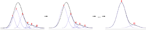
HODC:

• Input: Parameters for a mixture of Gaussian densities, that is, $\mathcal{P}$.

• Initialization: Set $m=0$ and $\mathbf{s}_{l}^{(0)}=\{l\}$, for $l=1,2,\ldots,L_{0}+L_{1}$;

• Repeat the following steps until $m=L_{0}+L_{1}-2$:

  • Step 1: Find

    $$l^{(m)}=\arg\min_{l}d\bigl{(}\widetilde{\phi}\bigl{(}\cdot;\mathbf{s}^{(m)}_{l},\mathcal{P}\bigr{)},\widetilde{\phi}\bigl{(}\cdot;\mathbf{s}^{(m)}_{l+1},\mathcal{P}\bigr{)}\bigr{)}.$$

  • Step 2: For $l=1,2,\ldots,L_{0}+L_{1}-m-1$, set

    $$\mathbf{s}_{l}^{(m+1)}=\cases{\mathbf{s}_{l}^{(m)}&\quad\mbox{if } $l<l^{(m)}$,\vspace*{2pt}\cr\mathbf{s}_{l}^{(m)}\cup\mathbf{s}_{l+1}^{(m)}&\quad\mbox{if } $l=l^{(m)}$,\vspace*{2pt}\cr\mathbf{s}_{l+1}^{(m)}&\quad\mbox{if } $l>l^{(m)}$.}$$

  • Step 3: Set $m=m+1$.

• Output: $\{\mathbf{s}_{l}^{(m)}\}_{l=1}^{L_{0}+L_{1}-m}$ for $m=1,2,\ldots,L_{0}+L_{1}-2$.

Figure 1 illustrates the HODC algorithm. The algorithm stops when $m=L_{0}+L_{1}-2$, where the ordered density components are partitioned into two classes indexed by $\mathbf{s}^{(m)}_{1}$ and $\mathbf{s}^{(m)}_{2}$. This suggests that the number of indices in $\mathbf{s}_{k+1}^{(m)}$, denoted by $|\mathbf{s}_{k+1}^{(m)}|$, is an estimate for $L_{k}$ in model (2.2). By running the HODC, we can obtain one $L_{k}$ estimate for each posterior sample generated from a DPM fitting. We take the average of $L_{k}$ estimates over all the posterior samples as the input of NET-DPM-2. The HODC also provides an approximation to $f_{k}(r)$ in (6), that is, $\widetilde{\phi}(r;\mathbf{s}_{k+1}^{(m)},\mathcal{P})$. This implies that we can further simplify the computation with the algorithm in the following section.

Figure 1: An illustration of the HODC algorithm for six density components: the HODC starts with clustering densities 1 and 2 as a mixture density labeled as 7, since the “distance” between 1 and 2 is shorter than all other adjacent density pairs. Then the HODC computes the “distance” between densities 3 and 7, densities 3 and 4, …, to proceed the clustering. Following this procedure, the HODC ends up with clustering densities 1, 2, 3 as a mixture density (labeled as 8) and 4, 5, 6 as another mixture density (labeled as 10).

2.4.3 FMM guided by a DPM model fitting

From a DPM model fitting, we obtain $V$ posterior samples of the parameters for the marginal density of $\mathbf{r}$. We denote them as $\mathcal{P}_{v}=\{(\widehat{\mu}_{vg},\widehat{\sigma}^{2}_{vg},\widehat{p}_{vg})\}_{g=1}^{L_{v0}+L_{v1}}$, for $v=1,2,\ldots,V$. For each $\mathcal{P}_{v}$, the HODC algorithm partitions $L_{v0}+L_{v1}$ components into two classes, where the class-specific components are indexed by $\mathbf{a}_{v,0}$ and $\mathbf{a}_{v,1}$. This leads to $V$ approximations of $f_{k}(r)$, that is, $\widetilde{\phi}(r;\mathbf{a}_{v,k},\mathcal{P}_{v})$. Given $f_{k}(r)$, our proposed gene selection model reduces to

$$[r_{i}\mid z_{i}=k]\stackrel{{\scriptstyle\mathrm{i.i.d.}}}{{\sim}}f_{k}(r)$$ (16)

for $i=1,2,\ldots,n$ and $k=0,1$, and $\mathbf{z}$ follows (4). To make inference on the posterior distribution of $\mathbf{z}$ by combining all $V$ approximations of $f_{k}(r)$, we consider

$$\pi(\mathbf{z}\mid\mathbf{r})\approx\frac{1}{V}\sum_{v=1}^{V}\pi(\mathbf{z}\mid\mathbf{r},\widetilde{\bolds{\phi}}_{v}),$$ (17)

where $\widetilde{\bolds{\phi}}_{v}=\{\widetilde{\phi}(r;\mathbf{a}_{v,0},\mathcal{P}_{v}),\widetilde{\phi}(r;\mathbf{a}_{v,1},\mathcal{P}_{v})\}$. For each $v$, the full conditional of $z_{i}$ is given by

$$\pi(z_{i}=k\mid\mathbf{z}_{-i},\mathbf{r},\widetilde{\bolds{\phi}}_{v})$$

(18)

$$\quad\quad\propto\widetilde{\phi}(r_{i};\mathbf{a}_{v,k},\mathcal{P}_{v})\exp\biggl{(}\widetilde{\omega}_{i}\log(\pi_{k})+\varrho_{k}\sum_{j\neq i}\omega_{j}c_{ij}I[z_{j}=k]\biggr{)}.$$

We refer to this algorithm as NET-DPM-3 (see Section B.3 in the supplemental article [Zhao, Kang and Yu (2014)] for details). It is extremely fast with a moderate $V$. Since the marginal density is estimated without using the network information, it might introduce bias on the distribution of $z_{i}$ and underestimate the variability of $z_{i}$. From our experience, those issues do not affect the selection accuracy much. Some examples are provided in Section 4.

2.5 The choice of hyperparameters

To proceed NET-DPMs, we need to specify the hyperparameters $\bolds{\pi}$, $\bolds{\varrho}$ and $\bolds{\omega}$ in (4). We assume that $\bolds{\omega}$ is prespecified according to biological information. In this paper, we choose equal weight, that is, $\bolds{\omega}=\mathbf{1}_{n}$ without incorporating any biological prior knowledge. We suggest two approaches to choosing $\bolds{\pi}$ and $\bolds{\varrho}$: (1) we assign hyperpriors on $\bolds{\pi}$ and $\bolds{\varrho}$ and make posterior inference; (2) for a set of possible choices of $\bolds{\pi}$ and $\bolds{\varrho}$, we employ the Bayesian model averaging. The details are provided in Section C in the supplemental article [Zhao, Kang and Yu (2014)].

3 Application

To demonstrate the behavior of our method, we apply the proposed method to the analysis of the Spellman yeast cell cycle microarray data set [Spellman et al. (1998)]. The data set is intended to detect genes with periodic behavior along the procession of the cell cycle. It has been extensively used in the development of computational methods. The network is summarized from the Database of Interacting Proteins (DIP) [Xenarios et al. (2002)]. We use the high-confidence connections between yeast proteins from the DIP. Eventually, the network contains 2031 genes, where the mean, median, maximum and minimum edges per gene are 3.948, 2, 57 and 1, respectively.

There is no outcome variable in the cell-cycle data set. In this demonstration we focus on the selection of genes with periodic behavior in light of the network. It is known that such genes show different phase shifts along the cell cycle and may not be correlated with each other [Yu (2010)]. We first perform the Fisher’s exact $G$ test for periodicity [Wichert, Fokianos and Strimmer (2004)] for each gene. We then transform the $p$-values to normal quantiles, $r_{i}=-\Phi^{-1}(p_{i})$ for gene $i$. We apply the fully Bayesian inference (NET-DPM-1), one fast computation approach (NET-DPM-3) and the standard DPM model fitting (STD-DPM) to this data set. For the NET-DPM-1, set $\tau_{0}=10$, $\tau_{1}=2$; following the results by STD-DPM, set $\gamma_{k}=\overline{\mu}_{k},\xi_{k}^{2}=\overline{\sigma}_{k}^{2},\beta_{k}=10,\alpha_{k}=\overline{\sigma}^{2}_{k}/\xi_{k}^{2}+1$ with $k=0,1$, where $\{\overline{\mu}_{k}\}$ and $\{\overline{\sigma}^{2}_{k}\}$ are preliminary estimations by the STD-DPM. We also conduct a sensitivity analysis for the hyperparameters specification (see the details in Section E in the supplemental article [Zhao, Kang and Yu (2014)]) to verify the robustness of the proposed methods. For both methods, the choices of $\pi_{0}$ and $\bolds{\varrho}$ for the model averaging algorithm are $(0.75,0.8,0.85,0.9)$ and $(0.5,1,5,10,15)\times(0.5,1,5,10,15)$ with restriction $\varrho_{0}<\varrho_{1}$. We run all the algorithms 5000 iterations with 2000 burn-in. In this article, the standard DPM fitting is obtained by an R package: DPpackage and all the proposed algorithms are implemented in R.

Table 1 presents the gene selection results based on three methods in a two-by-two table format. The number of the “selected” genes by the NET-DPM-1, the NET-DPM-3 and the STD-DPM are 201, 216 and 114, respectively. The summation of the diagonal elements of the table comparing the NET-DPM-3 and the NET-DPM-1 is larger than that for NET-DPM-3 and the STD-DPM. This indicates a stronger agreement between the two algorithms for NET-DPM.

=260pt NET-DPM-1 STD-DPM Selected Unselected Selected Unselected NET-DPM-3    Selected 170 0046 100 0116    Unselected 031 1784 014 1801

Table 1: Gene selection results by the three methods for the cell cycle data set

Figure 2: A subnetwork composed of genes with periodic behavior. The subnetwork consists of 135 genes. Red nodes: genes functionally involved in the M-phase of cell cycle; blue node: genes functionally involved in the interphase of cell cycle; green nodes: genes functionally involved in both M and interphase of cell cycle.

We focus our discussion on the NET-DPM-3 results. After removing all unselected genes, as well as selected genes not connected to any other selected genes, 163 of the 216 genes fall into 11 subnetworks. Of the 11 subnetworks, 10 are very small, each containing 5 or less genes. The remaining subnetwork contains 135 genes. Considering the purpose of the study is to find genes with periodic behavior, and most such genes are functionally related and regulated by the cell cycle process, this result is expected. We present the subnetwork in Figure 2. Sixty-one of the 135 genes belong to the mitotic cell cycle process based on gene ontology [Ashburner et al. (2000)]. The yeast mitotic cell cycle can be roughly divided into the M phase and the interphase, which contains S and G phases [Ashburner et al. (2000)]. We do not further divide the interphase because the number of genes annotated to its descendant nodes are small. Among the 135 genes, 45 are annotated to the M phase, and 21 are annotated to the interphase. By coloring the M phase genes in red, the interphase genes in blue and the genes annotated to both phases in green, we see that the majority of the selected M phase genes are clustered on the subnetwork, while the selected interphase genes are somewhat scattered, with 7 falling into a small but tight cluster.

Figure 3: A portion of the subnetwork shown in Figure 2, together with the immediate neighbors of the selected genes. Upper panel: NET-DPM-3 results; lower panel: STD-DPM results. The node labels indicate the gene name; circles and triangles represent “selected” and “unselected” genes; colors denote the value of the normal quantiles; a star in superscript represents the genes functionally annotated to the cell cycle process. Dash lines denote connections to genes not shown in the figure.

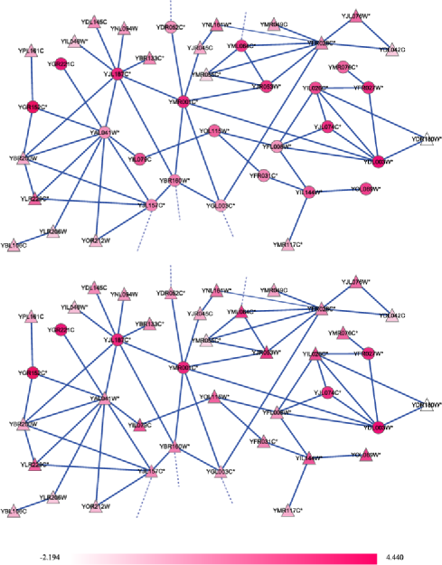
We show part of the subnetwork detected by the NET-DPM-3 with the corresponding one under the STD-DPM in Figure 3, where the genes that are linked by a dashed line are connected to other genes that are not shown in the figure. In this subnetwork, the gene selection results by the NET-DPM-1 agree with the NET-DPM-3 except for only one gene “YML064” for which the NET-DPM-1 does not select it with probability 0.478, while the NET-DPM-3 selects it with probability 0.687. This implies that both methods provide large uncertainty on this gene. Comparing the top panel (our method, NET-DPM-3) and bottom panel (STD-DPM), we observe a number of genes selected by NET-DPM but not by STD-DPM, and almost all such genes are cell cycle-related (denoted by a star by the ORF name). Examples include YAL041W (CLS4), which is required for the establishment and maintenance of polarity and critical in bud formation [Chenevert, Valtz and Herskowitz (1994); Cherry et al. (2012)]. The gene only shows moderate periodic behavior, as denoted by the color of the node. However, due to its links to other genes that have strong periodic behavior, it is selected by our method as an interesting gene. Another example is YFL008W (SMC1). It is a subunit of the cohesion complex, which is essential in sister chromatid cohesion of mitosis and meiosis. The complex is also involved in double-strand DNA break repair [Strunnikov and Jessberger (1999); Cherry et al. (2012)]. Similar to CLS4, the periodic behavior of SMC1 is not strong enough. It is only selected when the information is borrowed from linked genes that are functionally related and show strong periodic behavior. A number of other cell cycle-related genes in Figure 3 are in a similar situation, for example, YBR106W, YDR052C, YJL157C, YGL003C and YMR076C. These examples clearly show the benefit of utilizing the biological information stored in the network structure.

To assess the functional relevance of the selected genes globally, we resort to mapping the genes onto gene ontology biological processes [Ashburner et al. (2000)]. We limit our search to the GO Slim terms using the mapper of the Saccharomyces Genome Database [Cherry et al. (2012)]. The full result is listed in the supplementary file. Clearly, the overrepresented GO Slim terms are centered around cell cycle. Here we discuss some GO terms that are nonredundant. Among the 216 selected genes, 70 (32.4%, compared to 4.5% among all genes) belong to the process response to DNA damage stimulus (GO:0006974). The term shares a large portion of its genes with DNA recombination (GO:0006310) and DNA replication (GO:0006260) processes, which are integral to the cell cycle. Sixty-seven of the selected genes (31.0%, compared to 4.7% among all genes) belong to the process mitotic cell cycle (GO:0000278). Twenty-six of the 67 genes are shared with response to DNA damage stimulus (GO:0006974). Forty-one of the selected genes (19.0%, compared to 3.0% among all genes) belong to the process regulation of cell cycle (GO:0051726), among which 29 also belong to mitotic cell cycle (GO:0000278). Thirty-one of the selected genes (14.4%, compared to 2.6% among all genes) belong to the process meiotic cell cycle (GO:0051321), among which 12 are shared with mitotic cell cycle (GO:0000278). Other major enriched terms include chromatin organization (12.5%, compared to 3.5% overall), cytoskeleton organization (12.5%, compared to 3.4% overall), regulation of organelle organization (9.7%, compared to 2.4% overall) and cytokinesis (7.9%, compared to 1.7% overall). These terms clearly show strong relations with the yeast cell cycle.

4 Simulation studies

In this section we illustrate the performance of our methods (NET-DPMs) using simulation studies with various network structures and data settings compared with other methods. In Simulation 1 we study the similarity between the fully computational algorithm NET-DPM-1 and two fast computation approaches NET-DPM-$x$, $x=2,3$, in terms of gene selection accuracy and uncertainty estimations. Each of the three algorithms can be used along with one of the two methods for choosing hyperparameters: the posterior inference and model averaging. In Simulation 2 we focus on the gene network selection under a particular network structure and two types of simulated data to demonstrate the flexibility of the proposed methods. In both simulations we compare the NET-DPMs with a STD-DPM combined with the HODC algorithm without using any network information. In Section D in the supplemental article [Zhao, Kang and Yu (2014)], we also demonstrate the flexibility of the proposed methods by conducting a simulation on the selection of genes that are strongly associated with an outcome variable, and compare our NET-DPMs with a network based Bayesian variable selection (NET-BVS) proposed by Li and Zhang (2010).

Figure 4: Partial network structure with the dash lines representing connections to other nodes not shown in the figure.

4.1 Simulation 1

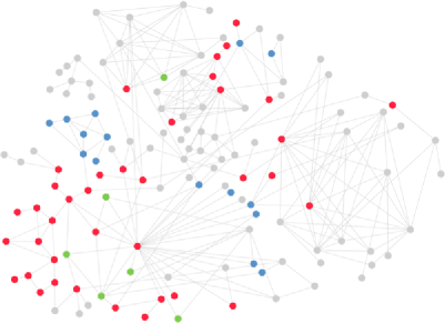
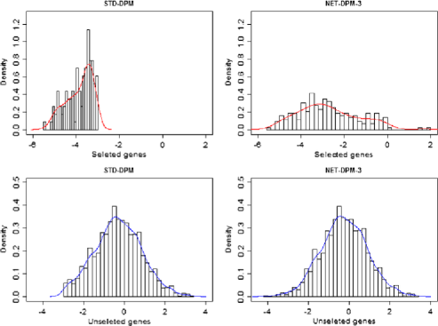
In this simulation we investigate the performance of the proposed algorithms using a simulated data set that mimic the real data in Section 3. We generate a scale-free network with 1000 genes based on the rich-get-rich algorithm [Barabási and Albert (1999)], that is, $n=1000$. Two hub genes with 64 and 69 connections to other genes are in this network; the mean and median edges per gene are 1.998 and 1. The partial network structure with the two hub genes included is shown in Figure 4. From the network structure, we generate $\mathbf{z}$ from the Ising model (4) with the sparsity parameter $\pi_{0}=0.8$ and smoothness parameters $\bolds{\varrho}=(\varrho_{0},\varrho_{1})=(5,10)$. For $i=1,\ldots,n$, in light of the results in Section 3, we simulate data $r_{i}$ given $z_{i}$ from the empirical distributions (Figure 5) of the test statistics for “selected” and “unselected” genes in the Spellman yeast cell cycle microarray data. As shown in Section 3, the NET-DPM-3 (Scenario 1) and the STD-DPM (Scenario 2) provide different gene selections results. We set both scenarios as the truth to simulate data.

Figure 5: Empirical distributions of “selected” genes (upper panel) and “unselected” genes (lower panel) in the Spellman yeast cell cycle data estimated by the NET-DPM-3 (right panel) and the STD-DPM (left panel).

We apply the NET-DPM-$x$, for $x=1,2,3$, and the STD-DPM to the simulated data set. To choose the sparsity and smoothness parameters, the NET-DPM-1 and the NET-DPM-3 are both combined with model averaging, where the possible choices of $\pi_{0}$ and $\bolds{\varrho}$ are $(0.75,0.8,0.85,0.9)$ and $(1,5,10,20,50)\times(1,5,10,20,50)$, while the NET-DPM-2 is combined with the posterior inference on $(\pi_{0},\bolds{\varrho})$. As for other hyperparameters, we specify $\tau_{k},\xi_{k},\gamma_{k},\beta_{k},\alpha_{k};k=0,1$ the same way as in the data application for the NET-DPM-$x$, for $x=1,2$. With random starting values, each algorithm is run 10 times under 10,000 iterations with 2000 burn-in. For each gene $i$, the mode of the marginal posterior probability of $z_{i}$ is taken to determine whether gene $i$ is selected or not. The selection performance for each method based on the average of the 10 runs is presented in Table 2. We also compare the posterior probability estimates of $\mathbf{z}$ between different algorithms under Scenario 1 in Figure 6.

Table 2: Gene selection accuracy in Simulation 1

	STD-DPM	NET-DPM-1	NET-DPM-2	NET-DPM-3
	Scenario 1
True positive rate	0.893	0.973	0.920	0.920
False positive rate	0.292	0.001	0.000	0.006
False discovery rate	0.801	0.014	0.000	0.080
	Scenario 2
True positive rate	1.000	1.000	1.000	1.000
False positive rate	0.232	0.000	0.000	0.007
False discovery rate	0.741	0.000	0.000	0.085
Typical computation time (hrs)	0.100	8.500	2.800	0.150

Figure 6: Marginal posterior probabilities of the class labels of all 1000 genes by the different methods: NET-DPM-3 vs. NET-DPM-2 (left panel) and NET-DPM-2 vs. NET-DPM-1 (right panel). The probability values are jittered by tiny random noises for better presenting.

Figure 7: Partial simulated gene network structure: the blue nodes represent “selected” genes and the red nodes represent “unselected” genes. Dash lines denote connections to genes not shown in the figure. A subnetwork of interest includes nodes 1, 2, 3, 4 and 5, which are encircled by a rectangle frame.

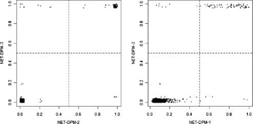
From Table 2, it is clear that the NET-DPMs achieve a better selection performance than the STD-DPM method under both scenarios. The STD-DPM without using the gene network information provides an extreme high false discovery rate in each scenario. This implies that it is critical to incorporate the gene network information to control FDR. Table 2 also suggests the NET-DPM-2 and the NET-DPM-3 approximate the NET-DPM-1 very well in terms of the gene selection accuracy with a substantial lower computational cost (3.4 GHz CPU, 8 GB Memory, Windows System). In addition, a comparison between the NET-DPM-2 and the NET-DPM-3 shows that the Bayesian model averaging over hyperparameters $(\pi_{0},\bolds{\varrho})$ provides an efficient alternative to the standard Bayesian posterior inference procedure. For the posterior probability estimates, the NET-DPM-2 and the NET-DPM-3 achieve a good agreement, as shown in the left panel of Figure 6. However, in the right panel of Figure 6, compared with the NET-DPM-1, the NET-DPM-3 tends to provide larger probability estimates for the “selected” genes, but smaller probability estimates for “unselected” genes. This implies the fast computation approaches underestimate the uncertainty of gene selection.

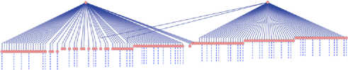
4.2 Simulation 2

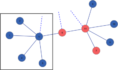
In this simulation we demonstrate the flexibility of the proposed methods and their ability to identify subnetworks of interest. We consider a 94-gene network which consists of an 11-gene subnetwork by design and an 83-gene scale-free network simulated from the rich-get-rich algorithm. The mean and median edges per node for the whole network are 2.02 and 1. Figure 7 shows the designed 11-gene subnetwork, where genes 5, 6 and 11 are connected with three other genes from the 83 gene scale-free network. Rather than simulating from priors, we directly specify the class label $\mathbf{z}$ as $z_{i}=1$ for $i\in\{1,2,3,4,5,8,9,10\}$, $z_{i}=0$ otherwise. In Figure 7 the blue nodes represent the “selected” genes and the red nodes are “unselected” genes. In addition, all other genes in the scale-free network (not shown in the figure) are “unselected.” The gene subnetwork of interest includes genes 1, 2, 3, 4 and 5, which are encircled by a rectangle frame in Figure 7. The null distribution for “unselected” $r_{i}$ is specified as a standard normal distribution: $[r_{i}\mid z_{i}=0]\sim\mathrm{N}(0,1)$. For the distribution of “selected” genes, we consider two settings:

Gaussian data: $$[r_{i}\mid z_{i}=1]\sim 0.4\times\mathrm{N}(3,1)+0.6\times\mathrm{N}(2,0.5),$$

Non-Gausian data: $$[r_{i}\mid z_{i}=1]\sim 0.4\times\mathrm{G}(5,2)+0.6\times\mathrm{G}(6,3),$$

where $\mathrm{G}(a,b)$ denotes a gamma distribution with shape $a$ and rate $b$. According to the above procedure, we simulate 100 data sets for each type of data. We apply the NET-DPM-3 and the STD-DPM to each data set. We utilize the model averaging for choosing hyperparameters and a set of possible choices are given by $\{1,2,5,10,15\}$ for both $\varrho_{0}$ and $\varrho_{1}$, and {0.8, 0.85, 0.9, 0.95} for $\pi_{0}$. We run 10,000 iterations with 2000 burn-in on each data set for both methods. In each simulated data set, we predetermine one gene as a “sure selected” gene. It has the largest number of connections with the “selected” genes estimated by the STD-DPM model.

Table 3 summarizes the selection accuracy of the gene subnetwork based on the 100 simulated data sets for each type of data. It is clear that the NET-DPM-3 provides much higher accuracy of the subnetwork selection than the STD-DPM. The NET-DPM-3 achieves a more than 60% accuracy rate in correctly identifying the subnetwork with an additional low false positive and false negative occurrences regardless of the type of data. This verifies the overall better performance of NET-DPM-3 than the STD-DPM in terms of identifying the gene subnetwork and the robustness of the proposed methods on different types of data.

Table 3: Selection accuracy of gene subnetworkta by TPR (true positive rate), FPR (false positive rate) and FDR (false discovery rate) in Simulation 2

	Gaussian data			Non-Gaussian data
Method	TPR	FPR	FDR	TPR	FPR	FDR
NET-DPM-3	63%	11%	15%	60%	05%	08%
STD-DPM	15%	33%	69%	17%	26%	60%

taFor gene subnetwork selection, the TPR is defined as the percentage of exactly selecting the correct network. The FPR is the percentage of selecting a larger network containing the correct network and at least one more other gene that has connection to the network. The FDR is the proportion of falsely selecting a larger network among all the network discoveries (selecting a correct or larger network).

5 Discussion

In the article we propose a Bayesian nonparametric mixture model for gene/gene subnetwork selection. Our model extends the standard DPM model incorporating the gene network information to significantly improve the accuracy of the gene selections and reduce the false discovery rate. We demonstrate that the proposed method has the ability to identify the subnetworks of genes and individual genes with a particular expressional behavior. We also show that it is able to select genes which are strongly associated with clinical variables. We develop a posterior computation algorithm along with two fast approximation approaches. The posterior inference can produce more accurate uncertainty estimates of gene selection, while the fast computing algorithms can achieve a similar gene selection accuracy. Due to the nonparametric nature, our method has the flexibility to fit various data types and has robustness to model assumptions.

When we observe gene expression data along with measurements of a clinical outcome, we need to create statistics to perform the selection of genes that are strongly associated with the clinical outcome. The choice of the statistics is crucial to the performance of our methods. To model the relationship between the clinical outcome and gene expression data, much literature suggests a linear regression model [Li and Li (2008); Pan, Xie and Shen (2010); Li and Zhang (2010); Stingo et al. (2011)], from which we produce testing statistics or coefficient estimates as the candidates. For instance, as we suggest in Section D in the supplemental article [Zhao, Kang and Yu (2014)], the most straightforward approach is to fit simple linear regression on each gene and use the $t$-statistics as the input data to our methods. However, there is no scientific evidence that the relationship between gene expression profiles and the clinical outcome should follow a linear regression model. Without making this assumption, we may test the independence between each gene expression profile and the clinical outcome via a nonparametric model suggested by Einmahl and Van Keilegom (2008) and use our model to fit the testing statistics. Other potential choices of statistics for the nonlinear problems include mutual information statistics [Peng, Long and Ding (2005)] and maximal information coefficient (MIC) statistics [Reshef et al. (2011)].

Although the development of our method is motivated by gene selection problems, our method can conduct variable selection for a general purpose and it has broad applications. For example, functional neuroimaging studies (e.g., fMRI and PET) usually produce large-scale statistics, one for each voxel in the brain. Those statistics are used to localize the brain activity regions related to particular brain functions. This essentially is a voxel selection problem to which our method is applicable, where the networks may be defined according to the spatial locations of the voxels. In addition to this, we discuss two future directions:

It is common that we have multiple hypothesis tests for each gene, and we have interest in jointly analyzing these statistics. This motivates an extension of the current NET-DPM model from one dimension to multiple dimensions for multivariate large-scale statistics.

The selection of one gene might be affected by not only the genes that are directly connected to it, but also the genes close to it over the network. It would be interesting to extend the prior specifications of the class label by incorporating a network distance. This should provide more biologically meaningful results.

References

- Antoniak (1974) {barticle}[mr] \bauthor\bsnmAntoniak, \bfnmCharles E.\binitsC. E. (\byear1974). \btitleMixtures of Dirichlet processes with applications to Bayesian nonparametric problems. \bjournalAnn. Statist. \bvolume2 \bpages1152–1174. \bidissn=0090-5364, mr=0365969 \bptokimsref\endbibitem
- Ashburner et al. (2000) {barticle}[pbm] \bauthor\bsnmAshburner, \bfnmM.\binitsM., \bauthor\bsnmBall, \bfnmC. A.\binitsC. A., \bauthor\bsnmBlake, \bfnmJ. A.\binitsJ. A., \bauthor\bsnmBotstein, \bfnmD.\binitsD., \bauthor\bsnmButler, \bfnmH.\binitsH., \bauthor\bsnmCherry, \bfnmJ. M.\binitsJ. M., \bauthor\bsnmDavis, \bfnmA. P.\binitsA. P., \bauthor\bsnmDolinski, \bfnmK.\binitsK., \bauthor\bsnmDwight, \bfnmS. S.\binitsS. S., \bauthor\bsnmEppig, \bfnmJ. T.\binitsJ. T., \bauthor\bsnmHarris, \bfnmM. A.\binitsM. A., \bauthor\bsnmHill, \bfnmD. P.\binitsD. P., \bauthor\bsnmIssel-Tarver, \bfnmL.\binitsL., \bauthor\bsnmKasarskis, \bfnmA.\binitsA., \bauthor\bsnmLewis, \bfnmS.\binitsS., \bauthor\bsnmMatese, \bfnmJ. C.\binitsJ. C., \bauthor\bsnmRichardson, \bfnmJ. E.\binitsJ. E., \bauthor\bsnmRingwald, \bfnmM.\binitsM., \bauthor\bsnmRubin, \bfnmG. M.\binitsG. M. and \bauthor\bsnmSherlock, \bfnmG.\binitsG. (\byear2000). \btitleGene ontology: Tool for the unification of biology. The Gene Ontology Consortium. \bjournalNat. Genet. \bvolume25 \bpages25–29. \biddoi=10.1038/75556, issn=1061-4036, mid=NIHMS269796, pmcid=3037419, pmid=10802651 \bptokimsref\endbibitem
- Barabási and Albert (1999) {barticle}[mr] \bauthor\bsnmBarabási, \bfnmAlbert-László\binitsA.-L. and \bauthor\bsnmAlbert, \bfnmRéka\binitsR. (\byear1999). \btitleEmergence of scaling in random networks. \bjournalScience \bvolume286 \bpages509–512. \biddoi=10.1126/science.286.5439.509, issn=0036-8075, mr=2091634 \bptokimsref\endbibitem
- Breeze et al. (2011) {barticle}[auto:STB—2014/02/12—14:17:21] \bauthor\bsnmBreeze, \bfnmE.\binitsE., \bauthor\bsnmHarrison, \bfnmE.\binitsE., \bauthor\bsnmMcHattie, \bfnmS.\binitsS., \bauthor\bsnmHughes, \bfnmL.\binitsL., \bauthor\bsnmHickman, \bfnmR.\binitsR., \bauthor\bsnmHill, \bfnmC.\binitsC., \bauthor\bsnmKiddle, \bfnmS.\binitsS., \bauthor\bsnmKim, \bfnmY.\binitsY., \bauthor\bsnmPenfold, \bfnmC.\binitsC., \bauthor\bsnmJenkins, \bfnmD.\binitsD. \betalet al. (\byear2011). \btitleHigh-resolution temporal profiling of transcripts during arabidopsis leaf senescence reveals a distinct chronology of processes and regulation. \bjournalThe Plant Cell Online \bvolume23 \bpages873–894. \bptokimsref\endbibitem
- Cerami et al. (2011) {barticle}[auto:STB—2014/02/12—14:17:21] \bauthor\bsnmCerami, \bfnmE.\binitsE., \bauthor\bsnmGross, \bfnmB.\binitsB., \bauthor\bsnmDemir, \bfnmE.\binitsE., \bauthor\bsnmRodchenkov, \bfnmI.\binitsI., \bauthor\bsnmBabur, \bfnmÖ.\binitsÖ., \bauthor\bsnmAnwar, \bfnmN.\binitsN., \bauthor\bsnmSchultz, \bfnmN.\binitsN., \bauthor\bsnmBader, \bfnmG.\binitsG. and \bauthor\bsnmSander, \bfnmC.\binitsC. (\byear2011). \btitlePathway commons, a web resource for biological pathway data. \bjournalNucleic Acids Res. \bvolume39 \bpagesD685–D690. \bptokimsref\endbibitem
- Chenevert, Valtz and Herskowitz (1994) {barticle}[auto:STB—2014/02/12—14:17:21] \bauthor\bsnmChenevert, \bfnmJ.\binitsJ., \bauthor\bsnmValtz, \bfnmN.\binitsN. and \bauthor\bsnmHerskowitz, \bfnmI.\binitsI. (\byear1994). \btitleIdentification of genes required for normal pheromone-induced cell polarization in saccharomyces cerevisiae. \bjournalGenetics \bvolume136 \bpages1287–1297. \bptokimsref\endbibitem
- Cherry et al. (2012) {barticle}[pbm] \bauthor\bsnmCherry, \bfnmJ. Michael\binitsJ. M., \bauthor\bsnmHong, \bfnmEurie L.\binitsE. L., \bauthor\bsnmAmundsen, \bfnmCraig\binitsC., \bauthor\bsnmBalakrishnan, \bfnmRama\binitsR., \bauthor\bsnmBinkley, \bfnmGail\binitsG., \bauthor\bsnmChan, \bfnmEsther T.\binitsE. T., \bauthor\bsnmChristie, \bfnmKaren R.\binitsK. R., \bauthor\bsnmCostanzo, \bfnmMaria C.\binitsM. C., \bauthor\bsnmDwight, \bfnmSelina S.\binitsS. S., \bauthor\bsnmEngel, \bfnmStacia R.\binitsS. R., \bauthor\bsnmFisk, \bfnmDianna G.\binitsD. G., \bauthor\bsnmHirschman, \bfnmJodi E.\binitsJ. E., \bauthor\bsnmHitz, \bfnmBenjamin C.\binitsB. C., \bauthor\bsnmKarra, \bfnmKalpana\binitsK., \bauthor\bsnmKrieger, \bfnmCynthia J.\binitsC. J., \bauthor\bsnmMiyasato, \bfnmStuart R.\binitsS. R., \bauthor\bsnmNash, \bfnmRob S.\binitsR. S., \bauthor\bsnmPark, \bfnmJulie\binitsJ., \bauthor\bsnmSkrzypek, \bfnmMarek S.\binitsM. S., \bauthor\bsnmSimison, \bfnmMatt\binitsM., \bauthor\bsnmWeng, \bfnmShuai\binitsS. and \bauthor\bsnmWong, \bfnmEdith D.\binitsE. D. (\byear2012). \btitleSaccharomyces Genome Database: The genomics resource of budding yeast. \bjournalNucleic Acids Res. \bvolume40 \bpagesD700–D705. \biddoi=10.1093/nar/gkr1029, issn=1362-4962, pii=gkr1029, pmcid=3245034, pmid=22110037 \bptokimsref\endbibitem
- Do, Müller and Tang (2005) {barticle}[mr] \bauthor\bsnmDo, \bfnmKim-Anh\binitsK.-A., \bauthor\bsnmMüller, \bfnmPeter\binitsP. and \bauthor\bsnmTang, \bfnmFeng\binitsF. (\byear2005). \btitleA Bayesian mixture model for differential gene expression. \bjournalJ. Roy. Statist. Soc. Ser. C \bvolume54 \bpages627–644. \biddoi=10.1111/j.1467-9876.2005.05593.x, issn=0035-9254, mr=2137258 \bptokimsref\endbibitem
- Dunson (2010) {bincollection}[mr] \bauthor\bsnmDunson, \bfnmDavid B.\binitsD. B. (\byear2010). \btitleNonparametric Bayes applications to biostatistics. In \bbooktitleBayesian Nonparametrics (\beditor\bfnmN. L.\binitsN. L. \bsnmHjort, \beditor\bfnmC.\binitsC. \bsnmHolmes, \beditor\bfnmP.\binitsP. \bsnmMüller and \beditor\bfnmS. G.\binitsS. G. \bsnmWalker, eds.) \bpages223–273. \bpublisherCambridge Univ. Press, \blocationCambridge. \bidmr=2730665 \bptokimsref\endbibitem
- Efron (2004) {barticle}[mr] \bauthor\bsnmEfron, \bfnmBradley\binitsB. (\byear2004). \btitleLarge-scale simultaneous hypothesis testing: The choice of a null hypothesis. \bjournalJ. Amer. Statist. Assoc. \bvolume99 \bpages96–104. \biddoi=10.1198/016214504000000089, issn=0162-1459, mr=2054289 \bptokimsref\endbibitem
- Efron (2010) {barticle}[mr] \bauthor\bsnmEfron, \bfnmBradley\binitsB. (\byear2010). \btitleCorrelated -values and the accuracy of large-scale statistical estimates. \bjournalJ. Amer. Statist. Assoc. \bvolume105 \bpages1042–1055. \biddoi=10.1198/jasa.2010.tm09129, issn=0162-1459, mr=2752597 \bptokimsref\endbibitem
- Einmahl and Van Keilegom (2008) {barticle}[mr] \bauthor\bsnmEinmahl, \bfnmJohn H. J.\binitsJ. H. J. and \bauthor\bsnmVan Keilegom, \bfnmIngrid\binitsI. (\byear2008). \btitleTests for independence in nonparametric regression. \bjournalStatist. Sinica \bvolume18 \bpages601–615. \bidissn=1017-0405, mr=2411617 \bptokimsref\endbibitem
- Escobar (1994) {barticle}[mr] \bauthor\bsnmEscobar, \bfnmMichael D.\binitsM. D. (\byear1994). \btitleEstimating normal means with a Dirichlet process prior. \bjournalJ. Amer. Statist. Assoc. \bvolume89 \bpages268–277. \bidissn=0162-1459, mr=1266299 \bptokimsref\endbibitem
- Escobar and West (1995) {barticle}[mr] \bauthor\bsnmEscobar, \bfnmMichael D.\binitsM. D. and \bauthor\bsnmWest, \bfnmMike\binitsM. (\byear1995). \btitleBayesian density estimation and inference using mixtures. \bjournalJ. Amer. Statist. Assoc. \bvolume90 \bpages577–588. \bidissn=0162-1459, mr=1340510 \bptokimsref\endbibitem
- Ishwaran and James (2001) {barticle}[mr] \bauthor\bsnmIshwaran, \bfnmHemant\binitsH. and \bauthor\bsnmJames, \bfnmLancelot F.\binitsL. F. (\byear2001). \btitleGibbs sampling methods for stick-breaking priors. \bjournalJ. Amer. Statist. Assoc. \bvolume96 \bpages161–173. \biddoi=10.1198/016214501750332758, issn=0162-1459, mr=1952729 \bptokimsref\endbibitem
- Ishwaran and James (2002) {barticle}[mr] \bauthor\bsnmIshwaran, \bfnmHemant\binitsH. and \bauthor\bsnmJames, \bfnmLancelot F.\binitsL. F. (\byear2002). \btitleApproximate Dirichlet process computing in finite normal mixtures: Smoothing and prior information. \bjournalJ. Comput. Graph. Statist. \bvolume11 \bpages508–532. \biddoi=10.1198/106186002411, issn=1061-8600, mr=1938445 \bptokimsref\endbibitem
- Jacob, Neuvial and Dudoit (2012) {barticle}[mr] \bauthor\bsnmJacob, \bfnmLaurent\binitsL., \bauthor\bsnmNeuvial, \bfnmPierre\binitsP. and \bauthor\bsnmDudoit, \bfnmSandrine\binitsS. (\byear2012). \btitleMore power via graph-structured tests for differential expression of gene networks. \bjournalAnn. Appl. Stat. \bvolume6 \bpages561–600. \biddoi=10.1214/11-AOAS528, issn=1932-6157, mr=2976483 \bptokimsref\endbibitem
- Leng and Müller (2006) {barticle}[pbm] \bauthor\bsnmLeng, \bfnmXiaoyan\binitsX. and \bauthor\bsnmMüller, \bfnmHans-Georg\binitsH.-G. (\byear2006). \btitleClassification using functional data analysis for temporal gene expression data. \bjournalBioinformatics \bvolume22 \bpages68–76. \biddoi=10.1093/bioinformatics/bti742, issn=1367-4803, pii=bti742, pmid=16257986 \bptokimsref\endbibitem
- Li and Li (2008) {barticle}[pbm] \bauthor\bsnmLi, \bfnmCaiyan\binitsC. and \bauthor\bsnmLi, \bfnmHongzhe\binitsH. (\byear2008). \btitleNetwork-constrained regularization and variable selection for analysis of genomic data. \bjournalBioinformatics \bvolume24 \bpages1175–1182. \biddoi=10.1093/bioinformatics/btn081, issn=1367-4811, pii=btn081, pmid=18310618 \bptokimsref\endbibitem
- Li and Zhang (2010) {barticle}[mr] \bauthor\bsnmLi, \bfnmFan\binitsF. and \bauthor\bsnmZhang, \bfnmNancy R.\binitsN. R. (\byear2010). \btitleBayesian variable selection in structured high-dimensional covariate spaces with applications in genomics. \bjournalJ. Amer. Statist. Assoc. \bvolume105 \bpages1202–1214. \biddoi=10.1198/jasa.2010.tm08177, issn=0162-1459, mr=2752615 \bptokimsref\endbibitem
- Ma et al. (2010) {barticle}[pbm] \bauthor\bsnmMa, \bfnmShuangge\binitsS., \bauthor\bsnmShi, \bfnmMingyu\binitsM., \bauthor\bsnmLi, \bfnmYang\binitsY., \bauthor\bsnmYi, \bfnmDanhui\binitsD. and \bauthor\bsnmShia, \bfnmBen-Chang\binitsB.-C. (\byear2010). \btitleIncorporating gene co-expression network in identification of cancer prognosis markers. \bjournalBMC Bioinformatics \bvolume11 \bpages271. \biddoi=10.1186/1471-2105-11-271, issn=1471-2105, pii=1471-2105-11-271, pmcid=2881088, pmid=20487548 \bptokimsref\endbibitem
- Müller and Quintana (2004) {barticle}[mr] \bauthor\bsnmMüller, \bfnmPeter\binitsP. and \bauthor\bsnmQuintana, \bfnmFernando A.\binitsF. A. (\byear2004). \btitleNonparametric Bayesian data analysis. \bjournalStatist. Sci. \bvolume19 \bpages95–110. \biddoi=10.1214/088342304000000017, issn=0883-4237, mr=2082149 \bptokimsref\endbibitem
- Neal (2000) {barticle}[mr] \bauthor\bsnmNeal, \bfnmRadford M.\binitsR. M. (\byear2000). \btitleMarkov chain sampling methods for Dirichlet process mixture models. \bjournalJ. Comput. Graph. Statist. \bvolume9 \bpages249–265. \biddoi=10.2307/1390653, issn=1061-8600, mr=1823804 \bptokimsref\endbibitem
- Pan, Xie and Shen (2010) {barticle}[mr] \bauthor\bsnmPan, \bfnmWei\binitsW., \bauthor\bsnmXie, \bfnmBenhuai\binitsB. and \bauthor\bsnmShen, \bfnmXiaotong\binitsX. (\byear2010). \btitleIncorporating predictor network in penalized regression with application to microarray data. \bjournalBiometrics \bvolume66 \bpages474–484. \biddoi=10.1111/j.1541-0420.2009.01296.x, issn=0006-341X, mr=2758827 \bptokimsref\endbibitem
- Peng, Long and Ding (2005) {barticle}[auto:STB—2014/02/12—14:17:21] \bauthor\bsnmPeng, \bfnmH.\binitsH., \bauthor\bsnmLong, \bfnmF.\binitsF. and \bauthor\bsnmDing, \bfnmC.\binitsC. (\byear2005). \btitleFeature selection based on mutual information criteria of max-dependency, max-relevance, and min-redundancy. \bjournalIEEE Trans. Pattern Analysis and Machine Intelligence \bvolume27 \bpages1226–1238. \bptokimsref\endbibitem
- Qu, Nettleton and Dekkers (2012) {barticle}[mr] \bauthor\bsnmQu, \bfnmLong\binitsL., \bauthor\bsnmNettleton, \bfnmDan\binitsD. and \bauthor\bsnmDekkers, \bfnmJack C. M.\binitsJ. C. M. (\byear2012). \btitleA hierarchical semiparametric model for incorporating intergene information for analysis of genomic data. \bjournalBiometrics \bvolume68 \bpages1168–1177. \biddoi=10.1111/j.1541-0420.2012.01778.x, issn=0006-341X, mr=3040023 \bptokimsref\endbibitem
- Reshef et al. (2011) {barticle}[pbm] \bauthor\bsnmReshef, \bfnmDavid N.\binitsD. N., \bauthor\bsnmReshef, \bfnmYakir A.\binitsY. A., \bauthor\bsnmFinucane, \bfnmHilary K.\binitsH. K., \bauthor\bsnmGrossman, \bfnmSharon R.\binitsS. R., \bauthor\bsnmMcVean, \bfnmGilean\binitsG., \bauthor\bsnmTurnbaugh, \bfnmPeter J.\binitsP. J., \bauthor\bsnmLander, \bfnmEric S.\binitsE. S., \bauthor\bsnmMitzenmacher, \bfnmMichael\binitsM. and \bauthor\bsnmSabeti, \bfnmPardis C.\binitsP. C. (\byear2011). \btitleDetecting novel associations in large data sets. \bjournalScience \bvolume334 \bpages1518–1524. \biddoi=10.1126/science.1205438, issn=1095-9203, mid=NIHMS358982, pii=334/6062/1518, pmcid=3325791, pmid=22174245 \bptokimsref\endbibitem
- Spellman et al. (1998) {barticle}[pbm] \bauthor\bsnmSpellman, \bfnmP. T.\binitsP. T., \bauthor\bsnmSherlock, \bfnmG.\binitsG., \bauthor\bsnmZhang, \bfnmM. Q.\binitsM. Q., \bauthor\bsnmIyer, \bfnmV. R.\binitsV. R., \bauthor\bsnmAnders, \bfnmK.\binitsK., \bauthor\bsnmEisen, \bfnmM. B.\binitsM. B., \bauthor\bsnmBrown, \bfnmP. O.\binitsP. O., \bauthor\bsnmBotstein, \bfnmD.\binitsD. and \bauthor\bsnmFutcher, \bfnmB.\binitsB. (\byear1998). \btitleComprehensive identification of cell cycle-regulated genes of the yeast Saccharomyces cerevisiae by microarray hybridization. \bjournalMol. Biol. Cell \bvolume9 \bpages3273–3297. \bidissn=1059-1524, pmcid=25624, pmid=9843569 \bptokimsref\endbibitem
- Stingo et al. (2011) {barticle}[mr] \bauthor\bsnmStingo, \bfnmFrancesco C.\binitsF. C., \bauthor\bsnmChen, \bfnmYian A.\binitsY. A., \bauthor\bsnmTadesse, \bfnmMahlet G.\binitsM. G. and \bauthor\bsnmVannucci, \bfnmMarina\binitsM. (\byear2011). \btitleIncorporating biological information into linear models: A Bayesian approach to the selection of pathways and genes. \bjournalAnn. Appl. Stat. \bvolume5 \bpages1978–2002. \biddoi=10.1214/11-AOAS463, issn=1932-6157, mr=2884929 \bptokimsref\endbibitem
- Strunnikov and Jessberger (1999) {barticle}[pbm] \bauthor\bsnmStrunnikov, \bfnmA. V.\binitsA. V. and \bauthor\bsnmJessberger, \bfnmR.\binitsR. (\byear1999). \btitleStructural maintenance of chromosomes (SMC) proteins: Conserved molecular properties for multiple biological functions. \bjournalEur. J. Biochem. \bvolume263 \bpages6–13. \bidissn=0014-2956, pii=ejb509, pmid=10429180 \bptokimsref\endbibitem
- Tang, Ghosal and Roy (2007) {barticle}[mr] \bauthor\bsnmTang, \bfnmYongqiang\binitsY., \bauthor\bsnmGhosal, \bfnmSubhashis\binitsS. and \bauthor\bsnmRoy, \bfnmAnindya\binitsA. (\byear2007). \btitleNonparametric Bayesian estimation of positive false discovery rates. \bjournalBiometrics \bvolume63 \bpages1126–1134, 1312. \biddoi=10.1111/j.1541-0420.2007.00819.x, issn=0006-341X, mr=2414590 \bptokimsref\endbibitem
- Wang and Dunson (2011) {barticle}[mr] \bauthor\bsnmWang, \bfnmLianming\binitsL. and \bauthor\bsnmDunson, \bfnmDavid B.\binitsD. B. (\byear2011). \btitleFast Bayesian inference in Dirichlet process mixture models. \bjournalJ. Comput. Graph. Statist. \bvolume20 \bpages196–216. \bnoteSupplementary material available online. \biddoi=10.1198/jcgs.2010.07081, issn=1061-8600, mr=2816545 \bptokimsref\endbibitem
- Wei and Li (2007) {barticle}[pbm] \bauthor\bsnmWei, \bfnmZhi\binitsZ. and \bauthor\bsnmLi, \bfnmHongzhe\binitsH. (\byear2007). \btitleA Markov random field model for network-based analysis of genomic data. \bjournalBioinformatics \bvolume23 \bpages1537–1544. \biddoi=10.1093/bioinformatics/btm129, issn=1367-4811, pii=btm129, pmid=17483504 \bptokimsref\endbibitem
- Wei and Li (2008) {barticle}[mr] \bauthor\bsnmWei, \bfnmZhi\binitsZ. and \bauthor\bsnmLi, \bfnmHongzhe\binitsH. (\byear2008). \btitleA hidden spatial-temporal Markov random field model for network-based analysis of time course gene expression data. \bjournalAnn. Appl. Stat. \bvolume2 \bpages408–429. \biddoi=10.1214/07–AOAS145, issn=1932-6157, mr=2415609 \bptokimsref\endbibitem
- Wei and Pan (2010) {barticle}[mr] \bauthor\bsnmWei, \bfnmPeng\binitsP. and \bauthor\bsnmPan, \bfnmWei\binitsW. (\byear2010). \btitleNetwork-based genomic discovery: Application and comparison of Markov random-field models. \bjournalJ. R. Stat. Soc. Ser. C. Appl. Stat. \bvolume59 \bpages105–125. \biddoi=10.1111/j.1467-9876.2009.00686.x, issn=0035-9254, mr=2750134 \bptokimsref\endbibitem
- Wei and Pan (2012) {barticle}[mr] \bauthor\bsnmWei, \bfnmPeng\binitsP. and \bauthor\bsnmPan, \bfnmWei\binitsW. (\byear2012). \btitleBayesian joint modeling of multiple gene networks and diverse genomic data to identify target genes of a transcription factor. \bjournalAnn. Appl. Stat. \bvolume6 \bpages334–355. \biddoi=10.1214/11-AOAS502, issn=1932-6157, mr=2951540 \bptokimsref\endbibitem
- Wichert, Fokianos and Strimmer (2004) {barticle}[pbm] \bauthor\bsnmWichert, \bfnmSofia\binitsS., \bauthor\bsnmFokianos, \bfnmKonstantinos\binitsK. and \bauthor\bsnmStrimmer, \bfnmKorbinian\binitsK. (\byear2004). \btitleIdentifying periodically expressed transcripts in microarray time series data. \bjournalBioinformatics \bvolume20 \bpages5–20. \bidissn=1367-4803, pmid=14693803 \bptokimsref\endbibitem
- Xenarios et al. (2002) {barticle}[pbm] \bauthor\bsnmXenarios, \bfnmIoannis\binitsI., \bauthor\bsnmSalwínski, \bfnmLukasz\binitsL., \bauthor\bsnmDuan, \bfnmXiaoqun Joyce\binitsX. J., \bauthor\bsnmHigney, \bfnmPatrick\binitsP., \bauthor\bsnmKim, \bfnmSul-Min\binitsS.-M. and \bauthor\bsnmEisenberg, \bfnmDavid\binitsD. (\byear2002). \btitleDIP, the Database of Interacting Proteins: A research tool for studying cellular networks of protein interactions. \bjournalNucleic Acids Res. \bvolume30 \bpages303–305. \bidissn=1362-4962, pmcid=99070, pmid=11752321 \bptokimsref\endbibitem
- Yu (2010) {barticle}[pbm] \bauthor\bsnmYu, \bfnmTianwei\binitsT. (\byear2010). \btitleAn exploratory data analysis method to reveal modular latent structures in high-throughput data. \bjournalBMC Bioinformatics \bvolume11 \bpages440. \biddoi=10.1186/1471-2105-11-440, issn=1471-2105, pii=1471-2105-11-440, pmcid=2940911, pmid=20799972 \bptokimsref\endbibitem
- Zhao, Kang and Yu (2014) {bmisc}[auto:STB—2014/02/12—14:17:21] \bauthor\bsnmZhao, \bfnmY.\binitsY., \bauthor\bsnmKang, \bfnmJ.\binitsJ. and \bauthor\bsnmYu, \bfnmT.\binitsT. (\byear2014) \bhowpublishedSupplement to “A Bayesian nonparametric mixture model for selecting genes and gene subnetworks.” DOI:\doiurl10.1214/14-AOAS719SUPP. \bptokimsref\endbibitem
- Zhou et al. (2010) {barticle}[mr] \bauthor\bsnmZhou, \bfnmBaiyu\binitsB., \bauthor\bsnmXu, \bfnmW.\binitsW., \bauthor\bsnmHerndon, \bfnmD.\binitsD., \bauthor\bsnmTompkins, \bfnmR.\binitsR., \bauthor\bsnmDavis, \bfnmR.\binitsR., \bauthor\bsnmXiao, \bfnmW.\binitsW., \bauthor\bsnmWong, \bfnmW.\binitsW., \bauthor\bsnmToner, \bfnmM.\binitsM., \bauthor\bsnmWarren, \bfnmH.\binitsH., \bauthor\bsnmSchoenfeld, \bfnmD.\binitsD. \betalet al. (\byear2010). \btitleAnalysis of factorial time-course microarrays with application to a clinical study of burn injury. \bjournalProc. Natl. Acad. Sci. USA \bvolume107 \bpages9923. \bptokimsref\endbibitem