Leveraging local identity-by-descent increases the power of case/control GWAS with related individuals

Abstract

Large case/control Genome-Wide Association Studies (GWAS) often include groups of related individuals with known relationships. When testing for associations at a given locus, current methods incorporate only the familial relationships between individuals. Here, we introduce the chromosome-based Quasi Likelihood Score (cQLS) statistic that incorporates local Identity-By-Descent (IBD) to increase the power to detect associations. In studies robust to population stratification, such as those with case/control sibling pairs, simulations show that the study power can be increased by over 50%. In our example, a GWAS examining late-onset Alzheimer’s disease, the $p$-values among the most strongly associated SNPs in the APOE gene tend to decrease, with the smallest $p$-value decreasing from $1.23\times 10^{-8}$ to $7.70\times 10^{-9}$. Furthermore, as a part of our simulations, we reevaluate our expectations about the use of families in GWAS. We show that, although adding only half as many unique chromosomes, genotyping affected siblings is more efficient than genotyping randomly ascertained cases. We also show that genotyping cases with a family history of disease will be less beneficial when searching for SNPs with smaller effect sizes.

copyrightownerIn the Public Domain

, , and t1Supported by the intramural program of the National Institute of Cancer. This study utilized the high-performance computational capabilities of the Biowulf Linux cluster at the National Institutes of Health, Bethesda, Md. (http://biowulf.nih.gov).

1 Introduction

Genome-Wide Association Studies (GWAS) of binary traits can include related individuals from known pedigrees [Barrett et al. (2008), Willer et al. (2008)]. In case–control studies, GWAS generally increase power by collecting cases with affected relatives, and may therefore find it cost-effective to genotype these related cases as well. Furthermore, GWAS may target families because the appropriate association tests are robust to population stratification [Ewens, Li and Spielman (2008)], the families have previously been collected for linkage analyses, the genetic variants can be called more accurately [Wang et al. (2007)], or the effects of parental imprinting can be evaluated [Wilkinson, Davies and Isles (2007)].

There are two general approaches for evaluating GWAS with related individuals from known pedigrees [Ott, Kamatani and Lathrop (2011), Manichaikul et al. (2012)]. The first approach combines two independent tests, a family-based test [Sham et al. (2002), Lange et al. (2003), Laird, Horvath and Xu (2000)], such as the transmission-disequilibrium test, and a population-based test of association. Methods exist for combining these two tests so the resulting analysis is robust to population stratification [Zheng et al. (2010), Won et al. (2012), Mirea et al. (2012), Manichaikul et al. (2012)]. The second approach, which potentially sacrifices robustness for improved power, calculates a single test statistic of association that accounts for the correlated genotypes among relatives [Bourgain et al. (2003), Thornton and McPeek (2007), Slager and Schaid (2001)]. Our focus is on the second approach and we derive a single test statistic which can use principal components [Price et al. (2006)] to correct for population stratification when necessary.

Until now, standard GWAS analyses have focused on the individual. For each individual, a study records their genotype and disease status. If all individuals were unrelated, the appropriate test statistic would simply be the correlation between an individual’s genotype and disease status [Hirschhorn and Daly (2005)]. However, when some individuals are related, a test statistic should correct for the dependence among genotypes and allow for the minor allele frequency (MAF) at a causal SNP to be higher in controls with affected relatives, as compared to randomly ascertained controls [Thornton and McPeek (2007), Bourgain et al. (2003), Zhu and Xiong (2012)]. The more-powerful Quasi-Likelihood Score (mQLS) statistic [Thornton and McPeek (2007)], an extension of the QLS [Bourgain et al. (2003)], accomplishes both objectives. However, because these statistics consider only the overall Identity By Descent (IBD) status between two individuals, they cannot allow for the MAF at a causal SNP to be higher in controls that share both alleles (IBD${}={}$2) with an affected sibling, as compared to controls that share no alleles (IBD${}={}$0) with an affected sibling.

We introduce a GWAS analysis that takes a different perspective and focuses on the founder chromosomes within each family. For each founder chromosome, we effectively identify its allele (at a given SNP) and the proportion of individuals carrying the SNP from that chromosome who are affected. This step is made possible by recent advances in IBD mapping and haplotyping [Browning and Browning (2010), Peters et al. (2012), He (2013)]. We suggest a chromosome-based Quasi Likelihood Score (cQLS) statistic that, at its simplest, measures the correlation between a binary indicator for the minor allele and the proportion of individuals affected. Formally, this test statistic is a partial score statistic from the retrospective likelihood that includes local IBD status among the observed data. The cQLS effectively leverages local IBD to improve power in GWAS with a large number of family-based controls. Furthermore, the derivation of the cQLS as a score statistic shows how to appropriately handle families of arbitrary pedigrees, include phenotype data from ungenotyped relatives, accommodate covariates, and allow for arbitrary models (e.g., logistic, liability threshold) linking disease risk and genotype status. In addition to these useful features, the cQLS also permits permutation-based measures of statistical significance. Accounting for relatedness in permutation methods of subject-centric approaches has proven exceptionally difficult [Wang (2011)].

In the next section, we define cQLS, describe the simulated data sets for testing its performance, and introduce a GWAS of Late-Onset Alzheimer’s Disease (LOAD) conducted by the National Institute of Aging and the National Cell Repository for Alzheimer’s Disease (NIA-LOAD/NCRAD) [Lee et al. (2008), Wijsman et al. (2011)]. In the third section, we evaluate the performance of the cQLS in simulated data sets and the NIA-LOAD/NCRAD data set. In addition to showing the potential benefit of cQLS, simulations evaluate the power gained by genotyping affected siblings, as compared to randomly ascertained cases, and demonstrate the diminished benefit of recruiting cases with a family history of disease when searching for SNPs with small effects [Ionita-Laza and Ottman (2011), Hattersley and McCarthy (2005), Teng and Risch (1999)]. In the final section, we conclude with a brief discussion.

2 Methods

2.1 cQLS: Definition

We consider a case–control study that contains $N_{\mathrm{Fam}}$ families, labeled $j=1,\ldots,N_{\mathrm{Fam}}$. Within family $j$, all genotyped chromosomes are assumed to arise from a family-specific set of $n_{j}$ founder chromosomes, labeled $k=1,\ldots,n_{j}$. We denote the total number of chromosomes by $N_{T}$:

$$N_{T}=\sum_{j}n_{j}.$$ (1)

For a given SNP, we let $Y_{jk}=1$ if the unique founder chromosome $k$ in family $j$ has a minor allele, and $Y_{jk}=0$ otherwise. Note that the subscripts “$j_{1}k$” and “$j_{2}k$” refer to different founder chromosomes from different families. For our discussion here, we will assume that $Y_{jk}$ is uniquely identifiable given the observed genetic data and that we can identify, with certainty, those individuals in family $j$ who inherited the SNP from founder chromosome $k$. Both assumptions will be relaxed in the Appendix. Furthermore, we will let $T_{jik^{\prime}k}=1$ if the $k^{\prime}$th copy ($k^{\prime}\in\{1,2\}$) of the specified SNP in individual $i$ is descended from founder chromosome $k$, and $T_{jik^{\prime}k}=0$ otherwise. We let $A_{ji}=1$ if individual $i$ is affected, and $A_{ji}=0$ otherwise.

For each founder SNP, we have $Y_{jk}$, indicating the presence or absence of a minor allele, and $C_{jk}=\sum_{i,k^{\prime}}T_{jik^{\prime}k}A_{ji}$, a count of the number of affected individuals with that SNP. If we expect that the minor allele increases disease risk, then the presence of a minor allele should be associated with a larger number of affected individuals. Therefore, the squared correlation between $Y_{jk}$ and $C_{jk}$ should be high. The proposed test statistic is a variation of this squared correlation.

Instead of using the count, $C_{jk}$, we use a version that normalizes each individual’s affection status to their expected affection status under the null hypothesis of no association,

$$Z_{jk}=\sum_{i}\sum_{k^{\prime}}T_{jik^{\prime}k}\biggl{(}A_{ji}-\frac{\hat{\pi}_{0}}{1-\hat{\pi}_{0}}(1-A_{ji})\biggr{)},$$ (2)

where $\hat{\pi}_{0}$ is our estimate of the prevalence of the disease in the population. We presume there are established estimates of $\hat{\pi}_{0}$ available in the literature. In the Appendix, we show how we can modify the expected affection status when other characteristics are known. We further show how we can make specific individuals, such as those with a family history of disease, carry more weight in the analysis by effectively increasing their contribution to $Z_{jk}$. We denote the average of all observed values of $Z_{jk}$ by

$$\bar{Z}\equiv\frac{\sum_{j,k}Z_{jk}}{N_{T}}.$$ (3)

Finally, we define a normalized version of the allele for chromosome $k$,

$$Y^{\dagger}_{jk}=Y_{jk}-\hat{\phi},$$ (4)

where

$$\hat{\phi}\equiv\frac{\sum_{j,k}Y_{jk}}{N_{T}}$$ (5)

and is our estimate of $\phi$, the minor allele frequency in the population, under the null hypothesis. As promised, our chromosome-based Quasi-Likelihood Score (cQLS) statistic is then proportional to the squared correlation between $Y^{\dagger}$ and $Z$,

$$\mathrm{cQLS}\equiv\frac{(\sum_{j,k}(Z_{jk}-\bar{Z})Y^{\dagger}_{jk})^{2}}{\sum_{j,k}(Z_{jk}-\bar{Z})^{2}\hat{\phi}(1-\hat{\phi})}.$$ (6)

Because $\operatorname{var}(Y^{\dagger}_{jk})$ is calculated as $\hat{\phi}(1-\hat{\phi})$, equation (6) requires the assumption of the Hardy–Weinberg Equilibrium (HWE). Therefore, the version of cQLS defined by equation (6) is appropriate in an ideal scenario where the genotypes and phenotypes of all individuals are known, $Y_{jk}$ can be identified for all families and chromosomes, and HWE holds. In the Appendix, we define a more robust cQLS that allows for violations in all three assumptions.

2.2 Assigning chromosomes

To calculate cQLS, we need to determine $T_{jik^{\prime}k}$, or the identity of the two chromosomes in individual $i$ for all $i,j,k^{\prime}$, and $k$ at each SNP. We perform this calculation in three steps. First, we phase subjects using BEAGLE [Browning and Browning (2011)], a software package for analysis of large-scale genetic data sets. Second, we detect shared segments within a family using GERMLINE [Gusev et al. (2009)], a software package for discovering long shared segments of Identity-By-Descent (IBD). In the third step, we convert the IBD status to $T_{jik^{\prime}k}$. The algorithm for this final step is described in Appendix B.4.

2.3 Simulations

Our three aims are to (1) assess the benefit of chromosome-based association tests (2) assess the value of genotyping an affected sibling and (3) assess the benefit of genotyping cases known to have affected siblings.

For our simulations, we assume that the liability threshold model accurately describes disease risk. In the liability threshold model, a complex disease results from an underlying, normally distributed, phenotype, or liability. When an individual’s liability exceeds a specific threshold, the individual is affected. In our scenario, the liability, $\mathbf{L}_{j}$, for individuals in nuclear family $j$ can be described by a linear function of their genotypes $\mathbf{G}_{j}$, where $G_{ji}$ is the number of minor alleles for individual $i$, $\mathbf{G}_{j}=[{G_{j1}\enskip\cdots\enskip G_{jN_{j}}}]^{t}$, and the superscript $t$ indicates transpose. Here, $\mathbf{E}_{j}$ accounts for environmental factors, while $\mathbf{F}_{j}$ accounts for background genetic correlation:

$$\mathbf{L}_{j}=\beta_{G}(\mathbf{G}_{j}-2\bolds{\phi})+\mathbf{E}_{j}+\beta_{F}\mathbf{F}_{j},$$ (7)

where

$$\left[\matrix{E_{j1}\vspace*{2pt}\cr E_{j2}\vspace*{2pt}\cr\vdots\vspace*{2pt}\cr E_{jN_{j}}}\right]\sim N\left(\left[\matrix{0\vspace*{2pt}\cr 0\vspace*{2pt}\cr\vdots\vspace*{2pt}\cr 0}\right],\left[\matrix{1&0&\cdots&0\vspace*{2pt}\cr 0&1&\cdots&0\vspace*{2pt}\cr\vdots\vspace*{2pt}\cr 0&0&\cdots&1}\right]\right)$$ (8)

and

$$\left[\matrix{F_{j1}\vspace*{2pt}\cr F_{j2}\vspace*{2pt}\cr F_{j3}\vspace*{2pt}\cr\vdots\vspace*{2pt}\cr F_{jN_{j}}}\right]\sim N\left(\left[\matrix{0\vspace*{2pt}\cr 0\vspace*{2pt}\cr 0\vspace*{2pt}\cr\vdots\vspace*{2pt}\cr 0}\right],\left[\matrix{1&0&0.5&\cdots&0.5\vspace*{2pt}\cr 0&1&0.5&\cdots&0.5\vspace*{2pt}\cr 0.5&0.5&1&\cdots&0.5\vspace*{2pt}\cr\vdots&\vdots&\vdots&\ddots&\vdots\vspace*{2pt}\cr 0.5&0.5&0.5&\cdots&1}\right]\right).$$ (9)

Here, $N_{j}$ is the number of individuals in family $j$, and individuals $j1$ and $j2$ are the parents. The liability threshold model will assign all individuals with $L_{ji}$ exceeding the population’s 95th percentile to have the disease. We chose $\beta_{G}$ so that the corresponding OR for each additional minor allele was between 1.02 and 1.36. We chose $\beta_{F}$ so that the sibling recurrence risk ratio, $\lambda_{S}$, was 1.5, 2 or 5 when $\beta_{G}=0$. Note that the magnitude of the sibling recurrence risk ratio, as defined here, is independent of the strength of the tested SNP. To calculate $\beta_{F}$, we numerically solved the following equation:

$$\int_{F_{2}^{-1}(0.95)}^{\infty}\biggl{[}\int_{F_{2}^{-1}(0.95)}^{\infty}f_{1}(x|y)\,\partial x\biggr{]}f_{2}(y)\,\partial y=0.05\lambda_{S},$$ (10)

where $F_{2}$ and $f_{2}$ are the cumulative distribution and density of $N(0,1+\beta^{2}_{F})$, and $f_{1}(x|y)$ is the density of $N(\beta^{2}_{F}y/(2(1+\beta^{2}_{F})),(1+2\beta^{2}_{F}+1.75\beta^{4}_{F})/(1+\beta^{2}_{F}))$. The MAF in the population was fixed at 0.1, and genotypes were simulated under HWE.

Our simulated studies, summarized in Table 1, collect families and/or unrelated cases and controls. The first five studies all start by identifying and genotyping 10,000 unrelated, randomly ascertained controls (R.A. controls). By randomly ascertained, we mean that we have no knowledge of their family history of disease. Study 1 further genotypes 5000 unrelated, randomly ascertained cases (R.A. cases). Study 2 genotypes 5000 unrelated cases (F.H. cases) with a family history of disease, specifically with an affected sibling. Study 3 genotypes both the 5000 R.A. cases and the 5000 F.H. cases. Study 4 genotypes 10,000 R.A. cases and 5000 F.H. cases. Studies 5 and 6 genotype 1 sibling of each proband. Study 5 genotypes the 5000 R.A cases, 5000 F.H. cases and their affected siblings. Study 6 includes 10,000 unrelated cases with an unaffected sibling and their unaffected siblings. Study 7 genotypes multiple relatives of each proband. Specifically, study 7 genotypes the 10,000 F.H. cases, their affected siblings and two unaffected siblings. Studies 6 and 7 highlight the potential power gain for cQLS in scenarios where only family-based controls are available.

Table 1: Each evaluated study design, labeled 1 through 7, genotypes different types of cases and controls. The first set of columns lists the number of randomly ascertained cases (Random), identified cases—or probands—with a family history (Fam. His.), and affected siblings of probands (Sib. 1) genotyped for the given study. The second set of columns lists the number of randomly ascertained controls (Rand.), unaffected “older” siblings (Sib. 1) and unaffected “younger” siblings (Sib. 2) genotyped for the given study. Studies 1 and 2 are used to assess the benefit of genotyping individuals with a family history of disease. Studies 3, 4 and 5 are used to assess the benefit of genotyping siblings of probands. Studies 6 and 7 are used to assess chromosome-based tests

	Cases			Controls
Study	Random	Fam. His.	Sib. 1	Random	Sib. 1	Sib. 2
1	0.5000	0000.0	0000.0	10,000	0000.0	0000.0
2	0000.0	0.5000	0000.0	10,000	0000.0	0000.0
3	0.5000	0.5000	0000.0	10,000	0000.0	0000.0
4	10,000	0.5000	0000.0	10,000	0000.0	0000.0
Multiple family members genotyped
5	0.5000	0.5000	0.5000	10,000	0000.0	0000.0
6	0000.0	10,000	0000.0	0000.0	10,000	0000.0
7	0000.0	10,000	10,000	0000.0	10,000	10,000

For various combinations of $\beta_{G}$, $\lambda_{S}$ and study design, we simulated 10,000 data sets and calculated the FBAT test statistic [Laird, Horvath and Xu (2000)], mQLS [Bourgain et al. (2003), Thornton and McPeek (2007)] and cQLS for each data set. The power was defined as the proportion of $p$-values that were below the $10^{-7}$ threshold, a common threshold for GWAS. By using 10,000 data sets, the standard errors for our estimates of power are bounded by 0.01. A short description of FBAT and mQLS are provided in Appendix A. Previous comparisons [Manichaikul et al. (2012)] of the available test statistics have demonstrated that, among currently available options, mQLS is consistently a top performer and the appropriate reference for comparison. For all simulations, the cQLS statistic was calculated using the true IBD of all chromosomes within each family. Moreover, the tested SNP was assumed to be the causal SNP. We also evaluated the effect of mistakes in IBD assignment on the power of the cQLS statistic. For a proportion of sibling sets, we randomly assigned the IBD status for each individual in that set, ensuring only that the IBD status was consistent with the observed genotypes. We then recalculated the power for Studies 6 and 7 with $\lambda_{S}=1.5$. We examined the scenarios where 2%, 5% and 8% of sibling sets were allowed to have errors.

To test the accuracy of the $p$-value, we simulated $10^{7}$ data sets under the null distribution for study designs 5, 6 and 7, where the mQLS and cQLS statistics differ, assuming $\lambda_{S}=5$. For computational efficiency, we included only 1000 subjects and only examined larger thresholds of $10^{-3}$ and $10^{-4}$.

2.4 NIA-LOAD

The details of the NIA-LOAD/NCRAD GWAS of Late Onset Alzheimer’s Disease (LOAD) have been described elsewhere [Wijsman et al. (2011)]. Briefly, the study recruited families with multiple affected individuals. Specifically, probands were required to have a diagnosis of Alzheimer’s Disease after the age of 60, have a sibling with a similar diagnosis and an additional biologically-related family member available for genotyping. In these families, additional relatives over the age of 50 were recruited regardless of cognitive status. Study participants were then genotyped using Illumina’s Human610Quadv1B BeadChips (Illumina, San Diego, CA, USA). We augmented the genotypes by imputing SNPs in the APOE region that have been previously associated with LOAD [Bertram et al. (2007)] using IMPUTE2 software version 2.2.2 [Howie, Donnelly and Marchini (2009)], with prephasing by SHAPEIT software version 1 [Delaneau, Zagury and Marchini (2013)] and version 3 of the 1000 Genomes Project data as the reference set. At each imputed SNP, we assigned the most likely genotypes that were consistent with IBD status. In order to create a study guaranteed to be robust to population stratification, we focused on 115 sets of siblings and pruned each set so that it had an equal number of cases and controls.

3 Results

3.1 cQLS vs mQLS

Chromosome-based test statistics had higher power, as compared to mQLS and FBAT, to detect associations when the study included cases and controls from the same family (Figure 1). We first consider simulations where the disease had a relatively low sibling relative risk of $\lambda_{S}=1.5$. If the GWAS included pairs of siblings (study 6), one affected and one unaffected, then a SNP that would be detected by cQLS in 75% of such studies would only be detected by QLS in 51% [Figure 1(a)]. In studies that included sets of four siblings (study 7), with each set including two affected and two unaffected individuals, when cQLS provided a power of 0.75, QLS provided a power of 0.36 [Figure 1(c)]. When we simulated a disease with a high sibling relative risk ($\lambda_{S}=5$), the power gained from using cQLS decreased. For study designs 6 and 7, mQLS achieved a power of 0.59 and 0.63 for SNPs where cQLS achieved a power of 0.75 [Figure 1(b), (d)].

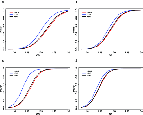
Figure 1: The power for cQLS (blue), mQLS (red) and FBAT (black) to detect the association between a SNP and the disease as a function of the OR when (a) $\lambda_{S}=1.5$ in study 6, (b) $\lambda_{S}=5$ in study 6, (c) $\lambda_{S}=1.5$ in study 7 and (d) $\lambda_{S}=5$ in study 7. Studies 6 and 7 correspond to genotyping pairs of siblings and groups of four siblings, respectively. $\lambda_{S}$ is the sibling relative risk of the disease.

Errors in IBD assignment decreased the power for association tests using cQLS. With an error rate of 2%, tests based on cQLS still had higher power for studies 6 and 7. However, with an error rate of 5%, cQLS performed no better than the other two test statistics in study 6 ($\lambda_{S}=1.5$). Specifically, when cQLS had a power of 0.75 (SE${}={}$0.01), QLS provided a similar power of 0.72 (SE${}={}$0.01). When the error rate reached 8%, the three test statistics performed similarly in study 7 ($\lambda_{S}=1.5$), with QLS achieving a power of 0.74 (0.01) when cQLS had a power of 0.75 (0.01).

Simulations suggest that the type-I error for the cQLS statistic matched the chosen $\alpha$ threshold when simulating data from the null distribution (Table 2).

Table 2: The proportions of $10^{7}$ null simulations where the cQLS, mQLS and FBAT $p$-values are below the specified $\alpha$ threshold. With $10^{7}$ simulations, the standard errors for our empirical $\alpha$-levels of $10^{-3}$ and $10^{-4}$ are approximately $10^{-5}=\sqrt{10^{-3}/10^{7}}$ and $3\times 10^{-6}=\sqrt{10^{-4}/10^{7}}$

	cQLS		mQLS		FBAT
Study	$\bolds{\alpha=10^{-3}}$	$\bolds{\alpha=10^{-4}}$	$\bolds{\alpha=10^{-3}}$	$\bolds{\alpha=10^{-4}}$	$\bolds{\alpha=10^{-3}}$	$\bolds{\alpha=10^{-4}}$
5	$9.81\times 10^{-4}$	$9.65\times 10^{-5}$	$9.79\times 10^{-4}$	$9.03\times 10^{-5}$	$9.44\times 10^{-4}$	$8.38\times 10^{-5}$
6	$9.80\times 10^{-4}$	$9.25\times 10^{-5}$	$1.00\times 10^{-3}$	$1.08\times 10^{-4}$	$9.56\times 10^{-4}$	$1.04\times 10^{-4}$
7	$9.70\times 10^{-4}$	$1.00\times 10^{-4}$	$9.78\times 10^{-4}$	$9.68\times 10^{-5}$	$9.62\times 10^{-4}$	$9.28\times 10^{-5}$

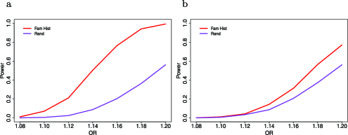
Figure 2: (a) The power to detect the association between a SNP and the disease, as a function of OR, when the study compares 10,000 randomly ascertained controls with either 5000 R.A. cases (red, study 1) or 5000 F.H. cases (blue, study 2) when the sibling relative risk, $\lambda_{S}$, is 1.5. (b) Same, but with $\lambda_{S}=5$. For tests of unrelated individuals, all QLS statistics give identical results.

3.2 Genotyping F.H. cases vs R.A. cases

Genotyping cases with a family history of disease provides a study with significantly higher power than genotyping randomly ascertained cases. For a disease with a low sibling relative risk ($\lambda_{S}=1.5$), when the effect size for a SNP was large enough so that the study with all F.H. cases (study 2) had a power of 0.75, a study with all R.A. cases (study 1) had a power of only 0.20 [Figure 2(a)]. However, as we increase the total heritability, shrinking the proportion of heritability attributable to the tested SNP, the power gained from using F.H. cases is decreased. When $\lambda_{S}=5$, a SNP with a power of 0.75 in study 2 would have had a power of 0.55 [Figure 2(b)] in study 1. For interpretation, recall that the sibling relative risk ($\lambda_{S}$) reflects the heritability from genetic variants other than the tested SNP. Therefore, as Figure 2(a) and 2(b) show, the power of study 1, which collects R.A. cases, does not depend on $\lambda_{S}$, but only on the relative risk of the tested SNP.

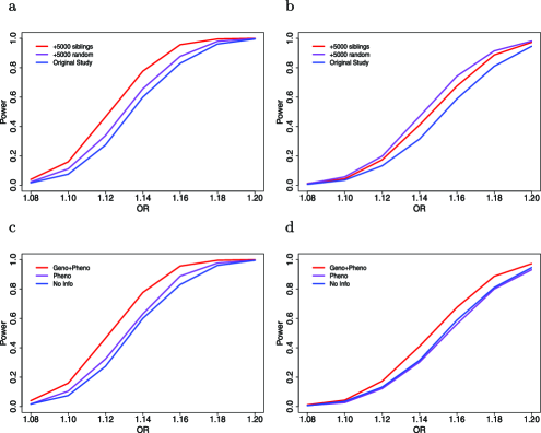
Figure 3: (a) The power to detect the association between a SNP and the disease, as a function of OR, when the study compares 10,000 randomly ascertained controls with either 5000 R.A. cases${}+{}$5000 F.H. cases (blue, study 3), 10,000 R.A. cases${}+{}$5000 F.H. cases (purple, study 4) or 5000 R.A. cases${}+{}$5000 pairs of affected siblings (red, study 5) given a sibling relative risk, $\lambda_{S}$, of 1.5 and all tests based on the score statistic. (b) Same, but with $\lambda_{S}=5$. (c) The power when the study compares 10,000 R.A. controls and either 5000 R.A. cases${}+{}$5000 F.H. cases and the score statistic (blue), 5000 R.A. cases${}+{}$5000 F.H. cases and cQLS (purple), or 5000 R.A. cases${}+{}$5000 pairs of affected siblings and the cQLS (red) given a sibling relative risk, $\lambda_{S}$, of 1.5. (d) Same, but with $\lambda_{S}=5$.

3.3 Genotyping affected sibling

Genotyping the affected siblings of F.H. cases increases the power. The additional genotyping of 5000 siblings, or moving from study 3 and a simple score test to study 5 and cQLS, will increase the power to detect a SNP with OR${}={}$1.15 from 0.57 to 0.75 [Figure 3(a)]. Each sibling, on average, only offers one new chromosome, but siblings are also F.H. cases and, as such, are enriched for the causal allele. Therefore, genotyping the 5000 siblings promises higher power than genotyping an additional 5000, unrelated, but randomly ascertained cases. Moving from study 3 to study 4, which includes 10,000 R.A. cases and 5000 F.H. cases, only increases the power from 0.57 to 0.63 [Figure 3(a)]. In studies with a mixture of F.H. cases and R.A. cases, such as study 3, the power of a standard association test can be improved by appropriately upweighting F.H. cases through use of either mQLS or cQLS. When moving from study 3 and cQLS to study 5 and cQLS, the power gain is less impressive, increasing from 0.60 to 0.75 [Figure 3(c)]. When the total heritability is high and $\lambda_{S}=5$, mQLS and cQLS overweight the F.H. cases, and including information about ungenotyped individuals can potentially lower power [Figure 3(d)].

3.4 LOAD

In addition to the simulations, we tested 11 SNPs in the APOE region of chromosome 19 for an association with LOAD in participants of the NIA-LOAD/NCRAD GWAS. Table 3 shows that eight of these 11 SNPs were associated with LOAD at a $p$-value below 0.05. In 7 of these 8 SNPs, the test based on the cQLS statistic resulted in a lower $p$-value, as compared to using the mQLS or FBAT statistic. However, all three methods provide similar evidence that these SNPs are associated with Alzheimer’s disease. For the two most strongly associated SNPs, rs429358 and rs4420638, the $p$-values were reduced from $1.23^{-8}$ and $5.23^{-7}$ based on the mQLS statistic, or $5.9^{-8}$ and $1.2^{-6}$ based on the FBAT statistic, to $7.70^{-9}$ and $1.79^{-7}$ based on the cQLS statistic.

Table 3: The $p$-values test from association tests of Late-Onset Alzheimer’s Disease and SNPs in the APOE region among the NIA-LOAD/NCRAD population. The first three columns indicate SNP ID, chromosome and position. The last three columns indicate the $p$-values calculated from the mQLS, FBAT and cQLS statistics

SNP	Chr.	Position	mQLS $\bolds{p}$-value	FBAT $\bolds{p}$-value	cQLS $\bolds{p}$-value
rs4806173	19	36,024,925	$8.5\times 10^{-1}$	$7.7\times 10^{-1}$	$9.1\times 10^{-1}$
rs12984928	19	36,029,852	$8.5\times 10^{-1}$	$7.7\times 10^{-1}$	$9.1\times 10^{-1}$
rs6857	19	45,392,254	$6.0\times 10^{-5}$	$5.8\times 10^{-6}$	$2.0\times 10^{-5}$
rs157582	19	45,396,219	$4.7\times 10^{-5}$	$4.8\times 10^{-6}$	$1.4\times 10^{-5}$
rs449647	19	45,408,564	$1.9\times 10^{-1}$	$2.1\times 10^{-1}$	$7.5\times 10^{-2}$
rs440446	19	45,409,167	$1.8\times 10^{-2}$	$2.4\times 10^{-2}$	$2.1\times 10^{-2}$
rs429358	19	45,411,941	$1.2\times 10^{-8}$	$5.9\times 10^{-8}$	$7.7\times 10^{-9}$
rs4420638	19	45,422,946	$5.2\times 10^{-7}$	$1.1\times 10^{-6}$	$1.8\times 10^{-7}$
rs157580	19	50,087,106	$3.9\times 10^{-2}$	$3.2\times 10^{-2}$	$1.8\times 10^{-2}$
rs2075650	19	50,087,459	$3.0\times 10^{-4}$	$7.1\times 10^{-5}$	$1.7\times 10^{-4}$
rs405509	19	50,100,676	$4.5\times 10^{-2}$	$2.3\times 10^{-2}$	$4.2\times 10^{-2}$

4 Discussion

Our primary objective was to introduce the chromosome-based Quasi-likelihood Score (cQLS) statistic and demonstrate that it can offer increased power to detect associations in GWAS with related individuals. Specifically, in studies designed to be robust to population stratification, such as those including sibling sets equally divided between cases and controls, statistical power can be increased by over 50%. The new statistic can also be applied to less robust study designs, but, like GWAS with unrelated individuals, would then require adjusting for population-eigenvectors. The derivation of cQLS as a partial likelihood shows how to easily adjust for covariates in both logistic and liability-threshold models.

Although our evaluation has focused on single SNP tests with fixed thresholds for statistical significance (e.g., $10^{-7}$), cQLS can offer a key, additional advantage when testing groups of SNPs in linkage disequilibrium. In GWAS with unrelated individuals, genotypes can be permuted among individuals to obtain permutation-based measures of significance. In GWAS with related individuals, standard methods are not appropriate, as individuals are not independent [Wang (2011)]. However, the founder chromosomes are independent and, therefore, it is straightforward to apply permutation methods with cQLS in GWAS of related individuals.

In addition to illustrating the improved power, we designed our simulations to reevaluate our expectations about the use of families in GWAS. First, affected siblings are often not genotyped because adding, on average, only one unique chromosome to the study is thought not to be worth the cost. However, we show that the power gained from genotyping an affected sibling can actually exceed the power from genotyping a randomly ascertained case. Second, it is well known that studies will have higher power when including cases (F.H. cases) with a family history of disease. F.H. cases should be enriched with disease-causing variants. However, we show that when a disease is highly heritable, the enrichment for any specific disease-causing variant is weaker. Thus, the benefit from genotyping cases with a family history of disease is lower, as demonstrated by our comparison of diseases with $\lambda_{S}=1.5$ and $\lambda_{S}=5$.

Like mQLS, cQLS offers the ability to use phenotyped, but not genotyped family members. Such an advantage could also be gained by imputing the genotype of such individuals and then performing the GWAS using the entire population, with appropriate adjustment for the uncertainty introduced by imputation. However such methods are not easily available and would still not offer the other benefit of cQLS, identifying local IBD.

Although cQLS requires calculating haplotypes for determining IBD, the test statistic still focuses on finding associations with single SNPs as opposed to haplotypes. A haplotype analysis [Akey, Jin and Xiong (2001)], which looks for associations with a specific haplotype, will decrease power when the causal SNP is directly genotyped, as is likely to be the case when using dense arrays or sequencing. However, having identified the haplotypes, this information can be used to adjust for local ancestry instead of using a more global principal components approach [Wang et al. (2011)].

The cQLS has limitations. First, the statistic will lose power in the presence of IBD error. In our examples, we found an error rate of 5% was large enough to offset the benefit of cQLS in the smaller studies. A second issue is that this new statistic requires a larger computational investment. Specifically, the first three steps of phasing, detecting shared segments of IBD and calculating $T_{jik^{\prime}k}$ required a total of 8.8 hours on a single 2.8 GHz Intel X5660 processor for the NIA-LOAD/NCRAD GWAS containing 575003 SNPs. After these initial steps, calculating the cQLS statistic for the NIA-LOAD/NCRAD GWAS required only 3.2 minutes. In comparison, mQLS required 70.4 minutes and FBAT required 11.1 minutes. Both mQLS and FBAT required less time by dividing the genome into 22 regions. For mQLS, we divided the genome into 22 intervals with an equal number of SNPs and for FBAT, we divided the genome into chromosomes. The mQLS program was not designed to handle GWAS, and we would expect that if optimized, performing an mQLS analysis would require less computational time than a cQLS analysis.

The benefit of cQLS depends on study design. For those designs that include mixtures of family-based and randomly ascertained controls, the increased power offered by cQLS will be lowered. Therefore, the additional computational cost would offer less value. Second, we have examined cQLS only in nuclear families and simple three-generation families (data not shown) where IBD can be reconstructed with high accuracy. We need further testing to assess the quality of IBD estimates from more distant relationships. Third, cQLS tests for association and, unlike FBAT, will have no power when there is linkage but no association. Although sequencing has removed our reliance on tag SNPs, a linkage analysis may still offer advantages in the presence of epistasis.

Finally, we remark that there is no consensus on how to best combine within-family and between-family information in GWAS with related individuals. However, a technical way to address this question would be to examine the full-data likelihood. The derivation of the cQLS (Appendix B) starts by defining this likelihood. The form of the final test statistic is the likelihood ratio test statistic based on the key partial likelihood, suggesting that the cQLS offers a near optimal combination of the two types of information.

Appendix A mQLS and FBAT

We compared the performance of a cQLS test to two standard tests: mQLS [Thornton and McPeek (2007)] and FBAT [Laird, Horvath and Xu (2000)]. mQLS is a quasi-likelihood score statistic that presumes an individual’s expected genotype increases with the sum, over all affected family members, of their kinship coefficients with that individual. A complete, but terse, definition follows.

For purposes of defining mQLS, we assume there are $n=N_{g}+M$ total subjects, of which $N_{g}$ have been genotyped. We let $\Phi$ be the $(N_{g}+M)\times(N_{g}+M)$ matrix of kinship coefficients and $\Phi_{N,M}$ be the submatrix containing the last $M$ columns of the first $N_{g}$ rows. The phenotype data are coded as $A^{{\ddagger}}$, a column vector of length $N_{g}+M$ having $i$th entry 1 if individual $i$ is affected, 0 if unknown and $\hat{\pi}_{0}/(1-\hat{\pi}_{0})$ otherwise. $A^{{\ddagger}}_{N}$ is the vector containing the first $N_{g}$ elements (e.g., genotyped individuals) and $A^{{\ddagger}}_{M}$ contains the last $M$ elements. Let $G$ be the vector of observed genotypes ($\frac{1}{2}G_{i}\in\{0,0.5,1\}$) for the first $N_{g}$ individuals. Finally, let $\mathbf{1}$ be a column vector of 1’s. Then mQLS is defined as

$$\mathrm{mQLS}=\hat{\sigma}^{-2}\bigl{(}\tfrac{1}{2}G-\hat{\mu}_{0}\bigr{)}^{T}\alpha\Gamma^{-1}\alpha^{T}\bigl{(}\tfrac{1}{2}G-\hat{\mu}_{0}\bigr{)},$$ (11)

where

$$\alpha = A^{{\ddagger}}_{N}+\Phi^{-1}\Phi_{N,M}A^{{\ddagger}}_{M},$$ (12)

$$\Gamma = \alpha^{T}\bigl{(}\Phi A^{{\ddagger}}_{n}+\Phi_{N,M}A^{{\ddagger}}_{M}\bigr{)}-\bigl{(}\mathbf{1}^{T}\alpha\bigr{)}^{2}\bigl{(}\mathbf{1}^{T}\Phi^{-1}\mathbf{1}^{T}\bigr{)}^{-1},$$ (13)

$$\hat{\mu}_{0} = \hat{p}_{\mathrm{null}}\mathbf{1},$$ (14)

$$\hat{\sigma}^{-2}_{0} = \bigl{[}\tfrac{1}{2}\hat{p}_{\mathrm{null}}(1-\hat{p}_{\mathrm{null}})\bigr{]}^{-1},$$ (15)

$$\hat{p}_{\mathrm{null}} = \tfrac{1}{2}\bigl{(}\mathbf{1}^{T}\Phi^{-1}\mathbf{1}\bigr{)}^{-1}\mathbf{1}^{T}\Phi^{-1}G.$$ (16)

For implementation, we downloaded the software from http://galton.uchicago.edu/~mcpeek/software/MQLS/index.html and, in simulations, set the prevalence of the disease to the “true” value.

FBAT compares the genotypes observed in the cases to their expected value under the null hypothesis of “no linkage and no association” or “no association, in the presence of linkage,” conditioned on the parent’s genotypes (or the appropriate sufficient statistic if parental genotypes are unknown). For details, we suggest the user’s manual for the software downloadable from http://www.biostat.harvard.edu/~fbat/default.html.

Appendix B cQLS: Derivation

B.1 Model assumptions

Without loss of generality, we can assume that all $N_{\mathrm{ind}}$ individuals come from the same family, and therefore drop the subscript $j$ from notation. We further define $\Theta$ to be the set of parameters in the model, including those defining the SNP’s effect on the disease. All notation and discussion assume a single SNP under study.

We will assume random mating.

We will assume

$$P[A_{i}=1|G_{i}=2,\mathbf{X}_{i},\Theta]=H_{i}^{2}P[A_{i}=1|G_{i}=0,\mathbf{X}_{i}\Theta],$$

where $G_{i}$ is defined as the genotype, or the number of minor alleles, for individual $i$, $\mathbf{X}_{i}$ is a vector of covariates, $\Theta$ is a set of parameters, and

$$H_{i}=\frac{P[A_{i}=1|G_{i}=1,\mathbf{X}_{i}]}{P[A_{i}=1|G_{i}=0,\mathbf{X}_{i}]}.$$ (17)

The immediate consequence is that

$$P[A_{i}=0|G_{i}=2,\mathbf{X}_{i},\Theta]=(1-\pi_{i})\biggl{[}\frac{1-H_{i}\pi_{i}}{1-\pi_{i}}\biggr{]}^{2}+\frac{\pi_{i}}{1-\pi_{i}}(H_{i}-1)^{2},$$

where $\pi_{i}$ is the probability individual $i$ is affected.

For purposes of deriving our test statistic, we further assume that $(\pi_{i}/(1-\pi_{i}))(H_{i}-1)^{2}$ is small or that we can treat the following approximation as an equality without issue:

$$P[A_{i}=0|G_{i}=2,\mathbf{X}_{i},\Theta]\approx\biggl{(}\frac{1-H_{i}\pi_{i}}{1-\pi_{i}}\biggr{)}^{2}P[A_{i}=0|G_{i}=0,\mathbf{X}_{i}].$$

The properties of the test statistic, such as being distributed as a $\chi^{2}_{1}$ variable under the null, will not depend on this approximation holding.

These approximations give us two simplifying results:

$$P\bigl{[}Y_{1},\ldots,Y_{n}|\mathbf{A},\mathbf{X},M^{*},\Theta\bigr{]} = \prod_{k}P\bigl{[}Y_{k}|\mathbf{A},\mathbf{X},M^{*},\Theta\bigr{]}$$ (18)

$$P\bigl{[}Y_{k}=1|\mathbf{A},\mathbf{X},M^{*},\Theta\bigr{]} = \frac{p\prod_{i}h_{i}^{\sum_{k^{\prime}}T_{ik^{\prime}k}}}{1+p\prod_{i}h_{i}^{\sum_{k^{\prime}}T_{ik^{\prime}k}}},$$ (19)

where $h_{i}=H_{i}A_{i}+(1-H_{i}\pi_{i})(1-\pi_{i})^{-1}(1-A_{i})$, $p=P[Y_{i}=1]/P[Y_{i}=0]=\phi/(1-\phi)$ and $M^{*}=\{T_{ik^{\prime}k}\dvtx i\in{1,\ldots,N_{\mathrm{ind}}},k^{\prime}\in\{1,2\},k\in\{1,\ldots,n\}\}$ is the IBD architecture. We will derive equations (18) and (19) in a later section of the Appendix.

B.2 Probability and score

We are interested in the distribution of $\mathbf{Y}$ and $\mathbf{M}^{O}$ given $\mathbf{A}$, $\mathbf{X}$, $S$ and $\Theta$. Here, $S$ is a vector indicating that the individuals were selected for the study and $\mathbf{M}^{O}$ are the observed values of $\mathbf{M}^{*}$. The variables $T_{ik^{\prime}k}$ cannot be identified in family members that are phenotyped, but not genotyped. We have chosen to treat $Y$ as the outcome because we will not need to know the selection procedure used to choose families and we do not need to estimate the nuisance parameter that is the correlation of disease status in the family due to nongenetic similarities. We do note that a full probability would be $P[\mathbf{Y},\mathbf{M}^{O},\mathbf{A},\mathbf{X}|S,\Theta]$ and we ignore $P[\mathbf{A},\mathbf{X}|S,\Theta]$ because it carries little information about $\Theta$:

$$P\bigl{[}\mathbf{Y},\mathbf{M}^{O}|\mathbf{A},\mathbf{X},S,\theta\bigr{]}=P\bigl{[}\mathbf{Y}|\mathbf{A},\mathbf{X},\mathbf{M}^{O},S,\theta\bigr{]}P\bigl{[}\mathbf{M}^{O}|\mathbf{A},\mathbf{X},S,\theta\bigr{]}.$$

However, we consider only the conditional probability, as this half is far more sensitive to $\Theta$. Also, although not mentioned above, we will make the additional assumption that, conditional on all other information, the genotypes and the characteristics used to select the individuals are independent. Then we know that $S$ drops out of the desired probability:

$$P\bigl{[}\mathbf{Y}|\mathbf{A},\mathbf{X},\mathbf{M}^{O},S,\Theta\bigr{]} = \frac{P[\mathbf{Y},S|\mathbf{A},\mathbf{X},\mathbf{M}^{O},\Theta]}{P[S|\mathbf{A},\mathbf{X},\mathbf{M}^{O},\Theta]}$$

$$= P\bigl{[}\mathbf{Y}|\mathbf{A},\mathbf{X},\mathbf{M}^{O},\Theta\bigr{]}.$$

In an upcoming section, we will show that the score statistic for $P[\mathbf{Y}|\mathbf{A},\mathbf{X},\break\mathbf{M}^{O},\Theta]$ is defined by equation (6) when $M^{*}$ is known.

B.3 Mathematical detail

B.3.1 Detail for Section B.1

We first demonstrate equation (18):

$$P\bigl{[}Y_{1},\ldots,Y_{n_{1}}|\mathbf{A},\mathbf{X},M^{*},\Theta\bigr{]}$$ (21)

$$\qquad=\frac{P[\mathbf{A}|Y_{1},\ldots,Y_{n_{1}},\mathbf{X},\Theta]\prod_{k}P[Y_{k}]}{P[\mathbf{A}|\mathbf{X},M^{*},\Theta]}$$ (22)

$$\qquad=\frac{P[\mathbf{A}|\mathbf{Y}=0,\mathbf{X},\Theta]\prod_{k}\prod_{i}h_{i}^{\sum_{k^{\prime}}G_{ik^{\prime}}T^{M^{*}}_{ik^{\prime}k}}P[Y_{k}]}{P[\mathbf{A}|M,\mathbf{X},\Theta]}$$ (23)

$$\qquad=\prod_{k}P[Y_{k}|\mathbf{A},M,\mathbf{X},\Theta].\vspace*{-1pt}$$ (24)

We next demonstrate equation (19), where we let $\mathbf{Y}_{-k}$ be the vector of all alleles except for $k$:

$$P\bigl{[}Y_{k}=1|\mathbf{A},\mathbf{X},M^{*},\Theta\bigr{]}$$ (31)

$$\qquad=P\bigl{[}Y_{k}=1|\mathbf{A},\mathbf{X},M^{*},\Theta,\mathbf{Y}_{-k}\bigr{]}$$

$$\qquad=\frac{P[\mathbf{A}|\mathbf{Y}_{-k},Y_{k}=1,\mathbf{X},M^{*},\Theta]P[Y_{k}=1]}{P[\mathbf{A}|\mathbf{Y}_{-k},\mathbf{X},M^{*},\Theta]}$$

$$\qquad=\biggl{(}\frac{P[\mathbf{A}|\mathbf{Y}_{-k},Y_{k}=1,\mathbf{X},M^{*},\Theta]}{P[\mathbf{A}|\mathbf{Y}_{-k},Y_{k}=0,\mathbf{X},M^{*},\Theta]}\frac{P[Y_{k}=1]}{P[Y_{k}=0]}$$

$$\hskip 6.0pt\qquad\quad{}\times P\bigl{[}\mathbf{A}|\mathbf{Y}_{-k},Y_{k}=0,\mathbf{X},M^{*},\Theta\bigr{]}P[Y_{k}=0]\biggr{)}$$

$$\qquad\quad{}\Big{/}{P\bigl{[}\mathbf{A}|\mathbf{Y}_{-k},\mathbf{X},M^{*},\Theta\bigr{]}}$$

$$\qquad=\frac{P[\mathbf{A}|\mathbf{Y}_{-k},Y_{k}=1,\mathbf{X},M^{*},\Theta]}{P[\mathbf{A}|\mathbf{Y}_{-k},Y_{k}=0,\mathbf{X},M^{*},\Theta]}\frac{P[Y_{k}=1]}{P[Y_{k}=0]}P\bigl{[}Y_{k}=0|\mathbf{A},\mathbf{X},M^{*},\Theta\bigr{]}$$

$$\qquad=\frac{\prod_{i}h_{i}^{\sum_{k^{\prime}}T_{ik^{\prime}k}}P[A_{i}|\mathbf{Y}_{-k},Y_{k}=0,\mathbf{X},M^{*},\Theta]}{\prod_{i}P[A_{i}|\mathbf{Y}_{-k},Y_{k}=0,\mathbf{X},M^{*},\Theta]}\frac{P[Y_{k}=1]}{P[Y_{k}=0]}$$

$$\qquad\quad{}\times P\bigl{[}Y_{k}=0|\mathbf{A},\mathbf{X},M^{*},\Theta\bigr{]}$$

$$\qquad=\prod_{i}h_{i}^{\sum_{k^{\prime}}T_{ik^{\prime}k}}\frac{P[Y_{k}=1]}{P[Y_{k}=0]}P\bigl{[}Y_{k}=0|\mathbf{A},\mathbf{X},M^{*},\Theta\bigr{]}.\vspace*{-1pt}$$

B.3.2 Score statistic: $Y_{jk}$ and $M^{*}$ can be uniquely identified

The overall probability can be written as the product of the probabilities for each chromosome with the assumptions in place:

$$P[\mathbf{Y}|D,p,\Theta]=\prod_{k}P[Y_{k}|D,p,\Theta],\vspace*{-1pt}$$ (32)

where $D$ abbreviates the collected data, $D=\{\mathbf{A},\mathbf{X},M^{*}\}$.

Because we must account for the nuisance parameter $p$, the score statistic for $\Theta$ is equation (B.3.2) evaluated under the null hypothesis

$$-\!\left[\matrix{\displaystyle\sum_{k}\frac{d}{d\Theta}\ell_{D}(Y_{k})&\displaystyle\sum_{k}\frac{d}{dp}\ell_{D}(Y_{k})}\right]$$

$$\qquad{}\times\left[\matrix{\displaystyle\sum_{k}\frac{d}{d^{2}\Theta}\ell_{D}(Y_{k})&\displaystyle\sum_{k}\frac{d}{d\Theta\,dp}\ell_{D}(Y_{k})\vspace*{2pt}\cr\displaystyle\sum_{k}\frac{d}{d\Theta\,dp}\ell_{D}(Y_{k})&\displaystyle\sum_{k}\frac{d}{d^{2}p}\ell_{D}(Y_{k})}\right]^{-1}\left[\matrix{\displaystyle\sum_{k}\frac{d}{d\Theta}\ell_{D}(Y_{k})\vspace*{2pt}\cr\displaystyle\sum_{k}\frac{d}{dp}\ell_{D}(Y_{k})}\right],$$

where

$$\ell_{D}(Y_{k})=\log\bigl{(}P\bigl{[}Y_{k}|\mathbf{A},\mathbf{X},M^{*},p,\Theta\bigr{]}\bigr{)}.$$ (34)

It is straightforward to evaluate the needed derivative

$$U \equiv \sum_{k}\frac{d}{d\Theta}\bigg{|}_{H_{0}}\ell_{D}(Y_{k})=\sum_{k}Z_{k}(Y_{k}-\hat{\phi}),$$ (35)

$$\hat{\phi} = \frac{\sum_{k}Y_{k}}{\sum_{k}1},$$ (36)

where

$$Z_{k} \equiv \sum_{i}\sum_{k^{\prime}}T_{ik^{\prime}k}\frac{\dot{h}_{i}}{h_{i}},$$ (37)

$$\dot{h}_{i} = \frac{d}{d\Theta}h_{i}.$$ (38)

We can rewrite $U$, so that we can calculate its variance, $\sigma^{2}_{U}$, without computing/inverting the matrix in equation (B.3.2):

$$U \equiv \sum_{k}\frac{d}{d\Theta}\bigg{|}_{H_{0}}\ell_{D}(Y_{k})=\sum_{k}(Z_{k}-\bar{Z})(Y_{k}-\hat{\phi}),$$ (39)

$$\bar{Z} = \frac{\sum_{k}Z_{k}}{\sum_{k}1},$$ (40)

$$\sigma^{2}_{U} = \phi(1-\phi)\sum_{k}(Z_{k}-\bar{Z})^{2}.$$ (41)

B.3.3 Score statistic: All individuals are not genotyped and $M^{*}$ cannot be uniquely identified

When all family members are not genotyped, the probability must be averaged over the $B$ possible IBD states

$$P\bigl{[}\mathbf{Y}|\mathbf{A},\mathbf{X},\mathbf{M}^{O},p,\Theta\bigr{]}$$

(42)

$$\qquad=\sum_{b=1}^{B}P\bigl{[}\mathbf{Y}|\mathbf{A},\mathbf{X},M^{*}=m_{b},p,\Theta\bigr{]}P\bigl{[}m_{b}|M^{O}\bigr{]}.$$

We can take advantage of the equality

$$\frac{d}{d\Theta}\bigg{|}_{H_{0}}\log\biggl{(}\sum_{b}c_{b}P\bigl{[}\mathbf{Y}|D(m_{b}),p,\Theta\bigr{]}\biggr{)}$$

(43)

$$\qquad=\frac{d}{d\Theta}\bigg{|}_{H_{0}}\sum_{b}c_{b}\log\bigl{(}P\bigl{[}\mathbf{Y}|D(m_{b}),p,\Theta\bigr{]}\bigr{)},$$

where we use the abbreviation $c_{b}=P[m_{b}|M^{O}]$ and use $D(m_{b})$ because $M^{*}$ is no longer known.

Equation (B.3.3) shows us that the score for $P[\mathbf{Y}|\mathbf{A},\mathbf{X},\mathbf{M}^{O},p,\Theta]$ is proportional to the score we would observe had there been $N_{M}$ families, where all families had the observed $\mathbf{Y}$ and $c_{b}N_{M}$ of those families had IBD structure $m_{b}$. Therefore, equation (35) still holds, so long as we now let

$$Z_{k}\equiv\sum_{i}\sum_{k^{\prime}}P[T_{ik^{\prime}k}=1]\frac{\dot{h}_{i}}{h_{i}}.$$ (44)

B.3.4 Score statistic: $Y_{jk}$ cannot be uniquely identified

In some scenarios, $Y_{k}$ cannot be uniquely identified given the available genetic information. In these scenarios, we must average the two possibilities to obtain the value of cQLS. As an example, this situation occurs in our simulated studies of sibling pairs. When two siblings have IBD${}={}$1 and are each heterozygous, we cannot determine whether the shared chromosome has the minor or common allele. We focus on this specific example to explain the needed adjustment.

Let $Q_{j}=1$ if the siblings have IBD${}={}$1 and are both heterozygous. Furthermore, in such a family, let $Y_{1}$, $Y_{2}$ and $Y_{3}$ denote the alleles on the chromosome uniquely in the first brother, in both brothers and uniquely in the second brother, respectively. Let $Z_{1}$, $Z_{2}$ and $Z_{3}$ be the disease variable for each of those chromosomes. We know

$$P\bigl{(}Q=1|A,X,M^{*},p,\Theta\bigr{)}$$ (45)

$$\qquad=P\bigl{(}\{Y_{1},Y_{2},Y_{3}\}=\{1,0,1\}|A,X,M^{*},p,\Theta\bigr{)}$$ (46)

$$\qquad\quad{}+P\bigl{(}\{Y_{1},Y_{2},Y_{3}\}=\{0,1,0\}|A,X,M^{*},p,\Theta\bigr{)}.$$ (47)

For families with $Q=1$, we must reevaluate their contribution to the score equations. Under the null hypothesis, we find

$$\frac{d\log(P(Q=1|A,X,M^{*},p,\Theta))}{dp}\bigg{|}_{H_{0}}$$

(48)

$$\qquad=(2-\phi)\frac{-{\phi^{2}}/{p^{2}}}{1-\phi}+(1+\phi)\frac{\phi}{p^{2}}$$

and

$$\frac{d\log(P(Q=1|A,X,M^{*},p,\Theta))}{d\Theta}\bigg{|}_{H_{0}}=(1-2\phi)Z_{2}.$$ (49)

Our new contributions to the score equations lead us to the following MLE of $\phi$:

$$\hat{\phi}=\frac{N_{1}+N_{3}}{N_{0}+N_{1}+N_{3}},$$ (50)

where

$$N_{0} = \sum_{j,k}1(Q_{j}=0)1(Y_{jk}=0),$$ (51)

$$N_{1} = \sum_{j,k}1(Q_{j}=0)1(Y_{jk}=1),$$ (52)

$$N_{3} = \sum_{j,k}1(Q_{j}=1).$$ (53)

Furthermore, we can rewrite $U$ as

$$U=\sum_{j,k:Q_{j}=1}(Z_{k}-\bar{Z})(Y_{k}-\hat{\phi})+\sum_{j:Q_{j}=0}(1-2\hat{\phi})(Z_{2}-\bar{Z})$$ (54)

and the score statistic as

$$\frac{U^{2}}{\hat{\sigma}^{2}_{U}},$$ (55)

where we let $p_{u}$ be the unique probabilities of each of the eight possible combinations of $\{Y_{1},Y_{2},Y_{3}\}$ when IBD${}={}$1, $Z_{j*}$ be the possible corresponding contributions from family $j$, and $\hat{\sigma}^{2}_{U}$ be the appropriate estimate of the variance under the null:

$$p_{u1} = \hat{\phi}^{3},$$ (56)

$$p_{u2} = \hat{\phi}^{2}(1-\hat{\phi}),$$ (57)

$$p_{u3} = \hat{\phi}(1-\hat{\phi})^{2},$$ (58)

$$p_{u4} = (1-\hat{\phi})^{3},$$ (59)

$$Z_{*j1} = \Biggl{(}\sum_{k=1}^{3}(Z_{k}-\bar{Z})(1-\hat{\phi})\Biggr{)}^{2},$$

$$Z_{*j2} = \Biggl{(}\sum_{k=1}^{3}(Z_{k}-\bar{Z})(1-\hat{\phi})-Z_{3}+\bar{Z}\Biggr{)}^{2}+\bigl{(}(Z_{2}-\bar{Z})(1-\phi)\bigr{)}^{2}$$

$${}+\Biggl{(}\sum_{k=1}^{3}(Z_{k}-\bar{Z})(1-\hat{\phi})-Z_{1}+\bar{Z}\Biggr{)}^{2},$$

$$Z_{*j3} = \Biggl{(}\sum_{k=1}^{3}(Z_{k}-\bar{Z})(1-\hat{\phi})-Z_{2}-Z_{3}+2\bar{Z}\Biggr{)}^{2}+\bigl{(}(Z_{2}-\bar{Z})(1-\phi)\bigr{)}^{2}$$

$${}+\Biggl{(}\sum_{k=1}^{3}(Z_{k}-\bar{Z})(1-\hat{\phi})-Z_{1}-Z_{2}+2\bar{Z}\Biggr{)}^{2},$$

$$Z_{*j4} = \sum_{k=1}^{3}\bigl{(}(Z_{k}-\bar{Z})(-\hat{\phi})\bigr{)}^{2}$$

and

$$\hat{\sigma}^{2}_{U}=\hat{\phi}(1-\hat{\phi})\sum_{j,k:\mathrm{IBD}(j)\neq 1}(Z_{k}-\bar{Z})^{2}+\sum_{j:\mathrm{IBD}(j)=1}\sum_{t=1}^{4}p_{ut}Z_{*jt}.$$ (60)

Accurate haplotyping would overcome this difficulty and allow us touniquely identify $Y_{jk}$. As we expect haplotyping to become standard practice in the very near future [Peters et al. (2012)], we expect that this step will soon be unnecessary.

B.3.5 Violation of the Hardy–Weinberg Equilibrium

Our estimate for the variance of $U$ in equation (41) assumes that the genotypes are in HWE. As an alternative, start by calculating the 16 possible values (one for each genotype) of $U=\sum_{k}(Z_{k}-\bar{Z})(Y_{k}-\hat{\phi})$ for each family $j$. The second step is to calculate the probability of each of the 16 genotypes. Given these probabilities and the possible values of $U$, it is straightforward to calculate the variance of $U$ for any family under the null hypothesis, conditional on IBD architecture. Currently, this alternative is only available for families with at most four founding chromosomes (e.g., nuclear families) and, therefore, the remaining goal is to estimate $p=\{p_{200},p_{110},p_{101},p_{020},p_{011},p_{002}\}$, where $p_{xyz}$ is the probability that the founding individuals include $x$, $y$ and $z$ individuals with genotypes $G_{i}=0$, $G_{i}=1$ and $G_{i}=2$. We estimate these six probabilities by effectively maximizing $P(Y|M^{O},p)$ with the constraints that $p_{xyz}\geq 0$ and that $0.25p_{110}+0.5p_{020}+0.5p_{101}+0.75p_{011}+p_{002}=\hat{\phi}$. Specifically, we minimize the following function:

$$2\biggl{(}\sum_{j}1(n_{j}=2)\biggr{)}(M_{2}V_{2}-A_{2})^{2}+3\biggl{(}\sum_{j}1(n_{j}=4)\biggr{)}(M_{3}V_{3}-A_{3})^{2}$$

(61)

$$\qquad{}+4\biggl{(}\sum_{j}1(n_{j}=4)\biggr{)}(M_{4}V_{4}-A_{4})^{2},$$

where $M_{4}$ is a $6\times 6$ identity matrix,

$$M_{2} = \left[\matrix{1&0.5&0.25&0&0&0\vspace*{2pt}\cr 0&0.5&0.5&1&0.5&0\vspace*{2pt}\cr 0&0&0.25&0&0.5&1}\right]\quad\mbox{and}$$

$$M_{3} = \left[\matrix{1&0.25&0&0&0&0\vspace*{2pt}\cr 0&0.5&0.5&0.5&0&0\vspace*{2pt}\cr 0&0&0.5&0.5&0.5&0\vspace*{2pt}\cr 0&0&0&0&0.25&1\vspace*{2pt}\cr 0&0.25&0&0&0.5&0}\right]$$

and $V_{2}$ is the vector estimating $\{P(\sum_{k}Y_{k}=0|n_{j}=2),P(\sum_{k}Y_{k}=1|n_{j}=2),P(\sum_{k}Y_{k}=2|n_{j}=2)\}$, $V_{3}$ estimates $\{P(\sum_{k}Y_{k}=0|n_{j}=3),P(\sum_{k}Y_{k}=1,W=1|n_{j}=3),P(\sum_{k}Y_{k}=2,W=1|n_{j}=3),P(\sum_{k}Y_{k}=3|n_{j}=3),\break P(\sum_{k}Y_{k}=2,W=0|n_{j}=3)\}$, $V_{4}$ estimates $\{P(\sum_{k}Y_{k}=0|n_{j}=4),\break P(\sum_{k}Y_{k}=1|n_{j}=4),P(\sum_{k}Y_{k}=1,G_{2}=1|n_{j}=4),P(\sum_{k}Y_{k}=1,G_{2}\neq 1|n_{j}=4),P(\sum_{k}Y_{k}=3|n_{j}=4),P(\sum_{k}Y_{k}=4|n_{j}=4)\}$, $W$ is a binary variable indicating whether all alleles are identifiable, and $\{G_{1},G_{2}\}$ are the founder genotypes.

B.4 Algorithm for assigning $T_{ijk^{\prime}k}$

We start by arbitrarily assigning numbers to the chromosomes of the founder individuals and trimming the family so that no two individuals have IBD${}={}$2. Founder individuals are defined to be the largest group possible such that all pairs of founder individuals have IBD${}={}$0. Let $A$ be initialized as the founder individuals.

Find an individual, $i_{3}$, in the compliment of $A$, that meets the first of the following possible criteria and follow the assignment mechanism. Add individual $i_{3}$ to $A$ and then repeat.

1. [(a)]

2. $i_{3}$ has IBD${}={}$1 with two individuals in $A$, say, $i_{1}$ and $i_{2}$, that are also IBD${}={}$1 with each other. Count the number of minor alleles, among individuals $i_{1}$, $i_{2}$ and $i_{3}$, at all loci in the shared region. Assume chromosomes in individuals $i_{1}$ and $i_{2}$ have been labeled as $\{1,2\}$ and $\{1,4\}$.

   1. [(a)]

   2. If (nearly) all counts are even, the chromosomes in individual $i_{3}$ are assigned as $\{2,4\}$.

   3. (Nearly). All counts are not even, and individual $i_{3}$ is either IBD${}={}$0 with all other individuals in $A$ or IBD${}={}$1 only with individuals who are IBD${}={}$1 with both $i_{1}$ and $i_{2}$. Then the chromosomes in $i_{3}$ are labeled as $\{1,X\}$, where $X$ is a new chromosome number.

   4. (Nearly). All counts are not even, and individual $i_{3}$ is IBD${}={}$1 with at least two more individuals in $A$, say, $i_{4}$ and $i_{5}$, that are IBD${}={}$1 with each other, but IBD${}={}$0 with both $i_{1}$ and $i_{2}$. Then the chromosomes in $i_{3}$ are labeled as $\{1,5\}$, where we assume the chromosomes in $i_{4}$ and $i_{5}$ are labeled as $\{5,6\}$ and $\{5,8\}$.

   5. (Nearly). All counts are not even, and individual $i_{3}$ is IBD${}={}$1 with exactly one other individual in $A$, say, $i_{4}$, that is IBD${}={}$0 with both $i_{1}$ and $i_{2}$. Then, we label $i_{3}$ as $\{1,5\}$, where the chromosomes in individuals $i_{4}$ have been labeled as $\{5,6\}$.

3. $i_{3}$ has IBD${}={}$1 with two individuals in $A$, say, $i_{2}$ and $i_{3}$, that share IBD${}={}$0 with each other.

   1. [(a)]

   2. Individual $i_{1}$ (or $i_{2}$) has IBD${}={}$1 with another individual in A, say, $i_{4}$, in $A$. Then, we label $i_{3}$ as $\{2,3\}$, where the chromosomes in individuals $i_{1}$, $i_{2}$ and $i_{4}$ have been labeled as $\{1,2\}$, $\{3,4\}$ and $\{1,6\}$.

   3. Individual $i_{1}$ and $i_{2}$ have IBD${}={}$0 with all other individuals in A. Then, we label $i_{3}$ as $\{1,3\}$, where the chromosomes in individuals $i_{1}$ and $i_{2}$ have been labeled as $\{1,2\}$ and $\{3,4\}$.

4. $i_{3}$ has IBD${}={}$1 with only one individual in $A$, say, $i_{1}$.

   1. [(a)]

   2. Individual $i_{1}$ has IBD${}={}$1 with another individual in $A$, say, $i_{2}$. Assign the chromosomes in individual $i_{3}$ as $\{2,X\}$, where the chromosomes in individuals $i_{1}$ and $i_{2}$ have been labeled as $\{1,2\}$ and $\{1,4\}$ and $X$ is a new chromosome number.

   3. Individual $i_{1}$ has IBD${}={}$0 with all other individuals in $A$. Assign the chromosomes in individual $i_{3}$ as $\{2,X\}$, where the chromosomes in individuals $i_{1}$ have been labeled as $\{1,2\}$ and X is a new chromosome number.

B.5 Limitations

The standard method for finding an optimal test statistic starts by defining the parameter of interest and then writing out the likelihood of the observed data given this, and possibly other, parameters. In the GWAS discussed here, such a likelihood would necessarily bridge the within-family and between-family information, and immediately show how the two pieces of information should be combined. Here, we have defined this likelihood and shown that the cQLS is derived as the score statistic to a specific partial likelihood. However, as that likelihood shows, we ignore information that can be derived from the observed IBD structure. For example, if all affected siblings are IBD${}={}$2 at a SNP, that provides some evidence of an association between SNP and disease. Although that information is minimal, we are currently looking into methods for capturing and including this independent information as well. By using only the partial likelihood, the cQLS is not guaranteed to result in the most powerful test.

References

- Akey, Jin and Xiong (2001) {barticle}[pbm] \bauthor\bsnmAkey, \bfnmJ.\binitsJ., \bauthor\bsnmJin, \bfnmL.\binitsL. and \bauthor\bsnmXiong, \bfnmM.\binitsM. (\byear2001). \btitleHaplotypes vs single marker linkage disequilibrium tests: What do we gain? \bjournalEur. J. Hum. Genet. \bvolume9 \bpages291–300. \biddoi=10.1038/sj.ejhg.5200619, issn=1018-4813, pmid=11313774 \bptokimsref\endbibitem
- Barrett et al. (2008) {bmisc}[pbm] \bauthor\bsnmBarrett, \bfnmJeffrey C.\binitsJ. C., \bauthor\bsnmHansoul, \bfnmSarah\binitsS., \bauthor\bsnmNicolae, \bfnmDan L.\binitsD. L., \bauthor\bsnmCho, \bfnmJudy H.\binitsJ. H., \bauthor\bsnmDuerr, \bfnmRichard H.\binitsR. H., \bauthor\bsnmRioux, \bfnmJohn D.\binitsJ. D., \bauthor\bsnmBrant, \bfnmSteven R.\binitsS. R., \bauthor\bsnmSilverberg, \bfnmMark S.\binitsM. S., \bauthor\bsnmTaylor, \bfnmKent D.\binitsK. D., \bauthor\bsnmBarmada, \bfnmM. Michael\binitsM. M., \bauthor\bsnmBitton, \bfnmAlain\binitsA., \bauthor\bsnmDassopoulos, \bfnmThemistocles\binitsT., \bauthor\bsnmDatta, \bfnmLisa Wu\binitsL. W., \bauthor\bsnmGreen, \bfnmTodd\binitsT., \bauthor\bsnmGriffiths, \bfnmAnne M.\binitsA. M., \bauthor\bsnmKistner, \bfnmEmily O.\binitsE. O., \bauthor\bsnmMurtha, \bfnmMichael T.\binitsM. T., \bauthor\bsnmRegueiro, \bfnmMiguel D.\binitsM. D., \bauthor\bsnmRotter, \bfnmJerome I.\binitsJ. I., \bauthor\bsnmSchumm, \bfnmL. Philip\binitsL. P., \bauthor\bsnmSteinhart, \bfnmA. Hillary\binitsA. H., \bauthor\bsnmTargan, \bfnmStephan R.\binitsS. R., \bauthor\bsnmXavier, \bfnmRamnik J.\binitsR. J., \borganizationNIDDK IBD Genetics Consortium, \bauthor\bsnmLibioulle, \bfnmCécile\binitsC., \bauthor\bsnmSandor, \bfnmCynthia\binitsC., \bauthor\bsnmLathrop, \bfnmMark\binitsM., \bauthor\bsnmBelaiche, \bfnmJacques\binitsJ., \bauthor\bsnmDewit, \bfnmOlivier\binitsO., \bauthor\bsnmGut, \bfnmIvo\binitsI., \bauthor\bsnmHeath, \bfnmSimon\binitsS., \bauthor\bsnmLaukens, \bfnmDebby\binitsD., \bauthor\bsnmMni, \bfnmMyriam\binitsM., \bauthor\bsnmRutgeerts, \bfnmPaul\binitsP., \bauthor\bsnmGossum, \bfnmAndré Van\binitsA. V., \bauthor\bsnmZelenika, \bfnmDiana\binitsD., \bauthor\bsnmFranchimont, \bfnmDenis\binitsD., \bauthor\bsnmHugot, \bfnmJean-Pierre\binitsJ.-P., \bauthor\bparticlede \bsnmVos, \bfnmMartine\binitsM., \bauthor\bsnmVermeire, \bfnmSeverine\binitsS., \bauthor\bsnmLouis, \bfnmEdouard\binitsE., \borganizationBelgian-French IBD Consortium, \borganizationWellcome Trust Case Control Consortium, \bauthor\bsnmCardon, \bfnmLon R.\binitsL. R., \bauthor\bsnmAnderson, \bfnmCarl A.\binitsC. A., \bauthor\bsnmDrummond, \bfnmHazel\binitsH., \bauthor\bsnmNimmo, \bfnmElaine\binitsE., \bauthor\bsnmAhmad, \bfnmTariq\binitsT., \bauthor\bsnmPrescott, \bfnmNatalie J.\binitsN. J., \bauthor\bsnmOnnie, \bfnmClive M.\binitsC. M., \bauthor\bsnmFisher, \bfnmSheila A.\binitsS. A., \bauthor\bsnmMarchini, \bfnmJonathan\binitsJ., \bauthor\bsnmGhori, \bfnmJilur\binitsJ., \bauthor\bsnmBumpstead, \bfnmSuzannah\binitsS., \bauthor\bsnmGwilliam, \bfnmRhian\binitsR., \bauthor\bsnmTremelling, \bfnmMark\binitsM., \bauthor\bsnmDeloukas, \bfnmPanos\binitsP., \bauthor\bsnmMansfield, \bfnmJohn\binitsJ., \bauthor\bsnmJewell, \bfnmDerek\binitsD., \bauthor\bsnmSatsangi, \bfnmJack\binitsJ., \bauthor\bsnmMathew, \bfnmChristopher G.\binitsC. G., \bauthor\bsnmParkes, \bfnmMiles\binitsM., \bauthor\bsnmGeorges, \bfnmMichel\binitsM. and \bauthor\bsnmDaly, \bfnmMark J.\binitsM. J. (\byear2008). \bhowpublishedGenome-wide association defines more than 30 distinct susceptibility loci for Crohn’s disease. Nat. Genet. 40 955–962. \biddoi=10.1038/ng.175, issn=1546-1718, mid=NIHMS53734, pii=ng.175, pmcid=2574810, pmid=18587394 \bptokimsref\endbibitem
- Bertram et al. (2007) {barticle}[pbm] \bauthor\bsnmBertram, \bfnmLars\binitsL., \bauthor\bsnmMcQueen, \bfnmMatthew B.\binitsM. B., \bauthor\bsnmMullin, \bfnmKristina\binitsK., \bauthor\bsnmBlacker, \bfnmDeborah\binitsD. and \bauthor\bsnmTanzi, \bfnmRudolph E.\binitsR. E. (\byear2007). \btitleSystematic meta-analyses of Alzheimer disease genetic association studies: The AlzGene database. \bjournalNat. Genet. \bvolume39 \bpages17–23. \biddoi=10.1038/ng1934, issn=1061-4036, pii=ng1934, pmid=17192785 \bptokimsref\endbibitem
- Bourgain et al. (2003) {barticle}[author] \bauthor\bsnmBourgain, \bfnmCatherine\binitsC., \bauthor\bsnmHoffjan, \bfnmSabine\binitsS., \bauthor\bsnmNicolae, \bfnmRaluca\binitsR., \bauthor\bsnmNewman, \bfnmDina\binitsD., \bauthor\bsnmSteiner, \bfnmLori\binitsL., \bauthor\bsnmWalker, \bfnmKaren\binitsK., \bauthor\bsnmReynolds, \bfnmRebecca\binitsR., \bauthor\bsnmOber, \bfnmCarole\binitsC. and \bauthor\bsnmMcPeek, \bfnmMary Sara\binitsM. S. (\byear2003). \btitleNovel case–control test in a founder population identifies -selectin as an atopy-susceptibility locus. \bjournalThe American Journal of Human Genetics \bvolume73 \bpages612–626. \bptokimsref\endbibitem
- Browning and Browning (2010) {barticle}[pbm] \bauthor\bsnmBrowning, \bfnmSharon R.\binitsS. R. and \bauthor\bsnmBrowning, \bfnmBrian L.\binitsB. L. (\byear2010). \btitleHigh-resolution detection of identity by descent in unrelated individuals. \bjournalAm. J. Hum. Genet. \bvolume86 \bpages526–539. \biddoi=10.1016/j.ajhg.2010.02.021, issn=1537-6605, pii=S0002-9297(10)00103-5, pmcid=2850444, pmid=20303063 \bptokimsref\endbibitem
- Browning and Browning (2011) {barticle}[pbm] \bauthor\bsnmBrowning, \bfnmBrian L.\binitsB. L. and \bauthor\bsnmBrowning, \bfnmSharon R.\binitsS. R. (\byear2011). \btitleA fast, powerful method for detecting identity by descent. \bjournalAm. J. Hum. Genet. \bvolume88 \bpages173–182. \biddoi=10.1016/j.ajhg.2011.01.010, issn=1537-6605, pii=S0002-9297(11)00011-5, pmcid=3035716, pmid=21310274 \bptokimsref\endbibitem
- Delaneau, Zagury and Marchini (2013) {barticle}[author] \bauthor\bsnmDelaneau, \bfnmOlivier\binitsO., \bauthor\bsnmZagury, \bfnmJean-Francois\binitsJ.-F. and \bauthor\bsnmMarchini, \bfnmJonathan\binitsJ. (\byear2013). \btitleImproved whole-chromosome phasing for disease and population genetic studies. \bjournalNat. Meth. \bvolume10 \bpages5–6. \bptokimsref\endbibitem
- Ewens, Li and Spielman (2008) {barticle}[pbm] \bauthor\bsnmEwens, \bfnmWarren J.\binitsW. J., \bauthor\bsnmLi, \bfnmMingyao\binitsM. and \bauthor\bsnmSpielman, \bfnmRichard S.\binitsR. S. (\byear2008). \btitleA review of family-based tests for linkage disequilibrium between a quantitative trait and a genetic marker. \bjournalPLoS Genet. \bvolume4 \bpagese1000180. \biddoi=10.1371/journal.pgen.1000180, issn=1553-7404, pmcid=2528965, pmid=18818728 \bptokimsref\endbibitem
- Gusev et al. (2009) {barticle}[pbm] \bauthor\bsnmGusev, \bfnmAlexander\binitsA., \bauthor\bsnmLowe, \bfnmJennifer K.\binitsJ. K., \bauthor\bsnmStoffel, \bfnmMarkus\binitsM., \bauthor\bsnmDaly, \bfnmMark J.\binitsM. J., \bauthor\bsnmAltshuler, \bfnmDavid\binitsD., \bauthor\bsnmBreslow, \bfnmJan L.\binitsJ. L., \bauthor\bsnmFriedman, \bfnmJeffrey M.\binitsJ. M. and \bauthor\bsnmPe’er, \bfnmItsik\binitsI. (\byear2009). \btitleWhole population, genome-wide mapping of hidden relatedness. \bjournalGenome Res. \bvolume19 \bpages318–326. \biddoi=10.1101/gr.081398.108, issn=1088-9051, pii=gr.081398.108, pmcid=2652213, pmid=18971310 \bptokimsref\endbibitem
- Hattersley and McCarthy (2005) {barticle}[author] \bauthor\bsnmHattersley, \bfnmAndrew T.\binitsA. T. and \bauthor\bsnmMcCarthy, \bfnmMark I.\binitsM. I. (\byear2005). \btitleWhat makes a good genetic association study? \bjournalThe Lancet \bvolume366 \bpages1315–1323. \bptokimsref\endbibitem
- He (2013) {barticle}[pbm] \bauthor\bsnmHe, \bfnmDan\binitsD. (\byear2013). \btitleIBD-Groupon: An efficient method for detecting group-wise identity-by-descent regions simultaneously in multiple individuals based on pairwise IBD relationships. \bjournalBioinformatics \bvolume29 \bpagesi162–i170. \biddoi=10.1093/bioinformatics/btt237, issn=1367-4811, pii=btt237, pmcid=3694672, pmid=23812980 \bptokimsref\endbibitem
- Hirschhorn and Daly (2005) {barticle}[pbm] \bauthor\bsnmHirschhorn, \bfnmJoel N.\binitsJ. N. and \bauthor\bsnmDaly, \bfnmMark J.\binitsM. J. (\byear2005). \btitleGenome-wide association studies for common diseases and complex traits. \bjournalNat. Rev. Genet. \bvolume6 \bpages95–108. \biddoi=10.1038/nrg1521, issn=1471-0056, pii=nrg1521, pmid=15716906 \bptokimsref\endbibitem
- Howie, Donnelly and Marchini (2009) {barticle}[pbm] \bauthor\bsnmHowie, \bfnmBryan N.\binitsB. N., \bauthor\bsnmDonnelly, \bfnmPeter\binitsP. and \bauthor\bsnmMarchini, \bfnmJonathan\binitsJ. (\byear2009). \btitleA flexible and accurate genotype imputation method for the next generation of genome-wide association studies. \bjournalPLoS Genet. \bvolume5 \bpagese1000529. \biddoi=10.1371/journal.pgen.1000529, issn=1553-7404, pmcid=2689936, pmid=19543373 \bptokimsref\endbibitem
- Ionita-Laza and Ottman (2011) {barticle}[pbm] \bauthor\bsnmIonita-Laza, \bfnmIuliana\binitsI. and \bauthor\bsnmOttman, \bfnmRuth\binitsR. (\byear2011). \btitleStudy designs for identification of rare disease variants in complex diseases: The utility of family-based designs. \bjournalGenetics \bvolume189 \bpages1061–1068. \biddoi=10.1534/genetics.111.131813, issn=1943-2631, pii=genetics.111.131813, pmcid=3213373, pmid=21840850 \bptokimsref\endbibitem
- Laird, Horvath and Xu (2000) {barticle}[author] \bauthor\bsnmLaird, \bfnmNan M.\binitsN. M., \bauthor\bsnmHorvath, \bfnmSteve\binitsS. and \bauthor\bsnmXu, \bfnmXin\binitsX. (\byear2000). \btitleImplementing a unified approach to family-based tests of association. \bjournalGenetic Epidemiology \bvolume19 \bpagesS36–S42. \bptokimsref\endbibitem
- Lange et al. (2003) {barticle}[pbm] \bauthor\bsnmLange, \bfnmChristoph\binitsC., \bauthor\bsnmSilverman, \bfnmEdwin K.\binitsE. K., \bauthor\bsnmXu, \bfnmXin\binitsX., \bauthor\bsnmWeiss, \bfnmScott T.\binitsS. T. and \bauthor\bsnmLaird, \bfnmNan M.\binitsN. M. (\byear2003). \btitleA multivariate family-based association test using generalized estimating equations: FBAT-GEE. \bjournalBiostatistics \bvolume4 \bpages195–206. \biddoi=10.1093/biostatistics/4.2.195, issn=1465-4644, pii=4/2/195, pmid=12925516 \bptokimsref\endbibitem
- Lee et al. (2008) {barticle}[author] \bauthor\bsnmLee, \bfnmJ. H.\binitsJ. H., \bauthor\bsnmCheng, \bfnmR.\binitsR., \bauthor\bsnmGraff-Radford, \bfnmN.\binitsN., \bauthor\bsnmForoud, \bfnmT.\binitsT. and \bauthor\bsnmR, \bfnmMayeux\binitsM. (\byear2008). \btitleAnalyses of the national institute on aging late-onset Alzheimer’s disease family study: Implication of additional loci. \bjournalArchives of Neurology \bvolume65 \bpages1518–1526. \bptokimsref\endbibitem
- Manichaikul et al. (2012) {barticle}[author] \bauthor\bsnmManichaikul, \bfnmAni\binitsA., \bauthor\bsnmChen, \bfnmWei-Min\binitsW.-M., \bauthor\bsnmWilliams, \bfnmKayleen\binitsK., \bauthor\bsnmWong, \bfnmQuenna\binitsQ., \bauthor\bsnmSale, \bfnmMichale\binitsM., \bauthor\bsnmPankow, \bfnmJames\binitsJ., \bauthor\bsnmTsai, \bfnmMichael\binitsM., \bauthor\bsnmRotter, \bfnmJerome\binitsJ., \bauthor\bsnmRich, \bfnmStephen\binitsS. and \bauthor\bsnmMychaleckyj, \bfnmJosyf\binitsJ. (\byear2012). \btitleAnalysis of family- and population-based samples in cohort genome-wide association studies. \bjournalHuman Genetics \bvolume131 \bpages275–287. \bptokimsref\endbibitem
- Mirea et al. (2012) {barticle}[author] \bauthor\bsnmMirea, \bfnmLucia\binitsL., \bauthor\bsnmInfante-Rivard, \bfnmClaire\binitsC., \bauthor\bsnmSun, \bfnmLei\binitsL. and \bauthor\bsnmBull, \bfnmShelley B.\binitsS. B. (\byear2012). \btitleStrategies for genetic association analyses combining unrelated case–control individuals and family trios. \bjournalAmerican Journal of Epidemiology \bvolume176 \bpages70–79. \bptokimsref\endbibitem
- Ott, Kamatani and Lathrop (2011) {barticle}[pbm] \bauthor\bsnmOtt, \bfnmJurg\binitsJ., \bauthor\bsnmKamatani, \bfnmYoichiro\binitsY. and \bauthor\bsnmLathrop, \bfnmMark\binitsM. (\byear2011). \btitleFamily-based designs for genome-wide association studies. \bjournalNat. Rev. Genet. \bvolume12 \bpages465–474. \biddoi=10.1038/nrg2989, issn=1471-0064, pii=nrg2989, pmid=21629274 \bptokimsref\endbibitem
- Peters et al. (2012) {barticle}[author] \bauthor\bsnmPeters, \bfnmBrock A.\binitsB. A., \bauthor\bsnmKermani, \bfnmBahram G.\binitsB. G., \bauthor\bsnmSparks, \bfnmAndrew B.\binitsA. B., \bauthor\bsnmAlferov, \bfnmOleg\binitsO., \bauthor\bsnmHong, \bfnmPeter\binitsP., \bauthor\bsnmAlexeev, \bfnmAndrei\binitsA., \bauthor\bsnmJiang, \bfnmYuan\binitsY., \bauthor\bsnmDahl, \bfnmFredrik\binitsF., \bauthor\bsnmTang, \bfnmY. Tom\binitsY. T., \bauthor\bsnmHaas, \bfnmJuergen\binitsJ., \bauthor\bsnmRobasky, \bfnmKimberly\binitsK., \bauthor\bsnmZaranek, \bfnmAlexander Wait\binitsA. W., \bauthor\bsnmLee, \bfnmJe-Hyuk\binitsJ.-H., \bauthor\bsnmBall, \bfnmMadeleine Price\binitsM. P., \bauthor\bsnmPeterson, \bfnmJoseph E.\binitsJ. E., \bauthor\bsnmPerazich, \bfnmHelena\binitsH., \bauthor\bsnmYeung, \bfnmGeorge\binitsG., \bauthor\bsnmLiu, \bfnmJia\binitsJ., \bauthor\bsnmChen, \bfnmLinsu\binitsL., \bauthor\bsnmKennemer, \bfnmMichael I.\binitsM. I., \bauthor\bsnmPothuraju, \bfnmKaliprasad\binitsK., \bauthor\bsnmKonvicka, \bfnmKarel\binitsK., \bauthor\bsnmTsoupko-Sitnikov, \bfnmMike\binitsM., \bauthor\bsnmPant, \bfnmKrishna P.\binitsK. P., \bauthor\bsnmEbert, \bfnmJessica C.\binitsJ. C., \bauthor\bsnmNilsen, \bfnmGeoffrey B.\binitsG. B., \bauthor\bsnmBaccash, \bfnmJonathan\binitsJ., \bauthor\bsnmHalpern, \bfnmAaron L.\binitsA. L., \bauthor\bsnmChurch, \bfnmGeorge M.\binitsG. M. and \bauthor\bsnmDrmanac, \bfnmRadoje\binitsR. (\byear2012). \btitleAccurate whole-genome sequencing and haplotyping from 10 to 20 human cells. \bjournalNature \bvolume487 \bpages190–195. \bptokimsref\endbibitem
- Price et al. (2006) {barticle}[pbm] \bauthor\bsnmPrice, \bfnmAlkes L.\binitsA. L., \bauthor\bsnmPatterson, \bfnmNick J.\binitsN. J., \bauthor\bsnmPlenge, \bfnmRobert M.\binitsR. M., \bauthor\bsnmWeinblatt, \bfnmMichael E.\binitsM. E., \bauthor\bsnmShadick, \bfnmNancy A.\binitsN. A. and \bauthor\bsnmReich, \bfnmDavid\binitsD. (\byear2006). \btitlePrincipal components analysis corrects for stratification in genome-wide association studies. \bjournalNat. Genet. \bvolume38 \bpages904–909. \biddoi=10.1038/ng1847, issn=1061-4036, pii=ng1847, pmid=16862161 \bptokimsref\endbibitem
- Sham et al. (2002) {barticle}[author] \bauthor\bsnmSham, \bfnmPak C.\binitsP. C., \bauthor\bsnmPurcell, \bfnmShaun\binitsS., \bauthor\bsnmCherny, \bfnmStacey S.\binitsS. S. and \bauthor\bsnmAbecasis, \bfnmGonasalo R.\binitsG. R. (\byear2002). \btitlePowerful regression-based quantitative-trait linkage analysis of general pedigrees. \bjournalThe American Journal of Human Genetics \bvolume71 \bpages238–253. \bptokimsref\endbibitem
- Slager and Schaid (2001) {barticle}[author] \bauthor\bsnmSlager, \bfnmS. L.\binitsS. L. and \bauthor\bsnmSchaid, \bfnmD. J.\binitsD. J. (\byear2001). \btitleEvaluation of candidate genes in case–control studies: A statistical method to account for related subjects. \bjournalThe American Journal of Human Genetics \bvolume68 \bpages1457–1462. \bptokimsref\endbibitem
- Teng and Risch (1999) {barticle}[author] \bauthor\bsnmTeng, \bfnmJun\binitsJ. and \bauthor\bsnmRisch, \bfnmNeil\binitsN. (\byear1999). \btitleThe relative power of family-based and case–control designs for linkage disequilibrium studies of complex human diseases. II. Individual genotyping. \bjournalGenome Research \bvolume9 \bpages234–241. \bptokimsref\endbibitem
- Thornton and McPeek (2007) {barticle}[author] \bauthor\bsnmThornton, \bfnmTimothy\binitsT. and \bauthor\bsnmMcPeek, \bfnmMary Sara\binitsM. S. (\byear2007). \btitleCase–control association testing with related individuals: A more powerful quasi-likelihood score test. \bjournalThe American Journal of Human Genetics \bvolume81 \bpages321–337. \bptokimsref\endbibitem
- Wang (2011) {barticle}[pbm] \bauthor\bsnmWang, \bfnmZuoheng\binitsZ. (\byear2011). \btitleDirect assessment of multiple testing correction in case–control association studies with related individuals. \bjournalGenet. Epidemiol. \bvolume35 \bpages70–79. \biddoi=10.1002/gepi.20555, issn=1098-2272, pmid=21181898 \bptokimsref\endbibitem
- Wang et al. (2007) {barticle}[pbm] \bauthor\bsnmWang, \bfnmKai\binitsK., \bauthor\bsnmLi, \bfnmMingyao\binitsM., \bauthor\bsnmHadley, \bfnmDexter\binitsD., \bauthor\bsnmLiu, \bfnmRui\binitsR., \bauthor\bsnmGlessner, \bfnmJoseph\binitsJ., \bauthor\bsnmGrant, \bfnmStruan F. A.\binitsS. F. A., \bauthor\bsnmHakonarson, \bfnmHakon\binitsH. and \bauthor\bsnmBucan, \bfnmMaja\binitsM. (\byear2007). \btitlePennCNV: An integrated hidden Markov model designed for high-resolution copy number variation detection in whole-genome SNP genotyping data. \bjournalGenome Res. \bvolume17 \bpages1665–1674. \biddoi=10.1101/gr.6861907, issn=1088-9051, pii=gr.6861907, pmcid=2045149, pmid=17921354 \bptokimsref\endbibitem
- Wang et al. (2011) {barticle}[pbm] \bauthor\bsnmWang, \bfnmXuexia\binitsX., \bauthor\bsnmZhu, \bfnmXiaofeng\binitsX., \bauthor\bsnmQin, \bfnmHuaizhen\binitsH., \bauthor\bsnmCooper, \bfnmRichard S.\binitsR. S., \bauthor\bsnmEwens, \bfnmWarren J.\binitsW. J., \bauthor\bsnmLi, \bfnmChun\binitsC. and \bauthor\bsnmLi, \bfnmMingyao\binitsM. (\byear2011). \btitleAdjustment for local ancestry in genetic association analysis of admixed populations. \bjournalBioinformatics \bvolume27 \bpages670–677. \biddoi=10.1093/bioinformatics/btq709, issn=1367-4811, pii=btq709, pmcid=3042179, pmid=21169375 \bptokimsref\endbibitem
- Wijsman et al. (2011) {bmisc}[author] \bauthor\bsnmWijsman, \bfnmEllen M.\binitsE. M., \bauthor\bsnmPankratz, \bfnmNathan D.\binitsN. D., \bauthor\bsnmChoi, \bfnmYoonha\binitsY., \bauthor\bsnmRothstein, \bfnmJoseph H.\binitsJ. H., \bauthor\bsnmFaber, \bfnmKelley M.\binitsK. M., \bauthor\bsnmCheng, \bfnmRong\binitsR., \bauthor\bsnmLee, \bfnmJoseph H.\binitsJ. H., \bauthor\bsnmBird, \bfnmThomas D.\binitsT. D., \bauthor\bsnmBennett, \bfnmDavid A.\binitsD. A., \bauthor\bsnmDiaz-Arrastia, \bfnmRamon\binitsR., \bauthor\bsnmGoate, \bfnmAlison M.\binitsA. M., \bauthor\bsnmFarlow, \bfnmMartin\binitsM., \bauthor\bsnmGhetti, \bfnmBernardino\binitsB., \bauthor\bsnmSweet, \bfnmRobert A.\binitsR. A., \bauthor\bsnmForoud, \bfnmTatiana M.\binitsT. M., \bauthor\bsnmMayeux, \bfnmRichard\binitsR. and \borganizationNIA-LOAD/NCRAD Family Study Group (\byear2011). \bhowpublishedGenome-wide association of familial late-onset Alzheimer’s disease replicates BIN1 and CLU and nominates CUGBP2 in interaction with APOE. PLoS Genet. 7 e1001308. \bptokimsref\endbibitem
- Wilkinson, Davies and Isles (2007) {barticle}[pbm] \bauthor\bsnmWilkinson, \bfnmLawrence S.\binitsL. S., \bauthor\bsnmDavies, \bfnmWilliam\binitsW. and \bauthor\bsnmIsles, \bfnmAnthony R.\binitsA. R. (\byear2007). \btitleGenomic imprinting effects on brain development and function. \bjournalNat. Rev. Neurosci. \bvolume8 \bpages832–843. \biddoi=10.1038/nrn2235, issn=1471-0048, pii=nrn2235, pmid=17925812 \bptokimsref\endbibitem
- Willer et al. (2008) {barticle}[author] \bauthor\bsnmWiller, \bfnmCristen J.\binitsC. J., \bauthor\bsnmSanna, \bfnmSerena\binitsS., \bauthor\bsnmJackson, \bfnmAnne U.\binitsA. U., \bauthor\bsnmScuteri, \bfnmAngelo\binitsA., \bauthor\bsnmBonnycastle, \bfnmLori L.\binitsL. L., \bauthor\bsnmClarke, \bfnmRobert\binitsR., \bauthor\bsnmHeath, \bfnmSimon C.\binitsS. C., \bauthor\bsnmTimpson, \bfnmNicholas J.\binitsN. J., \bauthor\bsnmNajjar, \bfnmSamer S.\binitsS. S., \bauthor\bsnmStringham, \bfnmHeather M.\binitsH. M., \bauthor\bsnmStrait, \bfnmJames\binitsJ., \bauthor\bsnmDuren, \bfnmWilliam L.\binitsW. L., \bauthor\bsnmMaschio, \bfnmAndrea\binitsA., \bauthor\bsnmBusonero, \bfnmFabio\binitsF., \bauthor\bsnmMulas, \bfnmAntonella\binitsA., \bauthor\bsnmAlbai, \bfnmGiuseppe\binitsG., \bauthor\bsnmSwift, \bfnmAmy J.\binitsA. J., \bauthor\bsnmMorken, \bfnmMario A.\binitsM. A., \bauthor\bsnmNarisu, \bfnmNarisu\binitsN., \bauthor\bsnmBennett, \bfnmDerrick\binitsD., \bauthor\bsnmParish, \bfnmSarah\binitsS., \bauthor\bsnmShen, \bfnmHaiqing\binitsH., \bauthor\bsnmGalan, \bfnmPilar\binitsP., \bauthor\bsnmMeneton, \bfnmPierre\binitsP., \bauthor\bsnmHercberg, \bfnmSerge\binitsS., \bauthor\bsnmZelenika, \bfnmDiana\binitsD., \bauthor\bsnmChen, \bfnmWei-Min\binitsW.-M., \bauthor\bsnmLi, \bfnmYun\binitsY., \bauthor\bsnmScott, \bfnmLaura J.\binitsL. J., \bauthor\bsnmScheet, \bfnmPaul A.\binitsP. A., \bauthor\bsnmSundvall, \bfnmJouko\binitsJ., \bauthor\bsnmWatanabe, \bfnmRichard M.\binitsR. M., \bauthor\bsnmNagaraja, \bfnmRamaiah\binitsR., \bauthor\bsnmEbrahim, \bfnmShah\binitsS., \bauthor\bsnmLawlor, \bfnmDebbie A.\binitsD. A., \bauthor\bsnmBen-Shlomo, \bfnmYoav\binitsY., \bauthor\bsnmDavey-Smith, \bfnmGeorge\binitsG., \bauthor\bsnmShuldiner, \bfnmAlan R.\binitsA. R., \bauthor\bsnmCollins, \bfnmRory\binitsR., \bauthor\bsnmBergman, \bfnmRichard N.\binitsR. N., \bauthor\bsnmUda, \bfnmManuela\binitsM., \bauthor\bsnmTuomilehto, \bfnmJaakko\binitsJ., \bauthor\bsnmCao, \bfnmAntonio\binitsA., \bauthor\bsnmCollins, \bfnmFrancis S.\binitsF. S., \bauthor\bsnmLakatta, \bfnmEdward\binitsE., \bauthor\bsnmLathrop, \bfnmG Mark\binitsG. M., \bauthor\bsnmBoehnke, \bfnmMichael\binitsM., \bauthor\bsnmSchlessinger, \bfnmDavid\binitsD., \bauthor\bsnmMohlke, \bfnmKaren L.\binitsK. L. and \bauthor\bsnmAbecasis, \bfnmGoncalo R.\binitsG. R. (\byear2008). \btitleNewly identified loci that influence lipid concentrations and risk of coronary artery disease. \bjournalNat. Genet. \bvolume40 \bpages161–169. \bptokimsref\endbibitem
- Won et al. (2012) {barticle}[pbm] \bauthor\bsnmWon, \bfnmSungho\binitsS., \bauthor\bsnmLu, \bfnmQing\binitsQ., \bauthor\bsnmBertram, \bfnmLars\binitsL., \bauthor\bsnmTanzi, \bfnmRudolph E.\binitsR. E. and \bauthor\bsnmLange, \bfnmChristoph\binitsC. (\byear2012). \btitleOn the meta-analysis of genome-wide association studies: A robust and efficient approach to combine population and family-based studies. \bjournalHum. Hered. \bvolume73 \bpages35–46. \biddoi=10.1159/000331219, issn=1423-0062, pii=000331219, pmcid=3322629, pmid=22261799 \bptokimsref\endbibitem
- Zheng et al. (2010) {barticle}[mr] \bauthor\bsnmZheng, \bfnmYingye\binitsY., \bauthor\bsnmHeagerty, \bfnmPatrick J.\binitsP. J., \bauthor\bsnmHsu, \bfnmLi\binitsL. and \bauthor\bsnmNewcomb, \bfnmPolly A.\binitsP. A. (\byear2010). \btitleOn combining family-based and population-based case–control data in association studies. \bjournalBiometrics \bvolume66 \bpages1024–1033. \biddoi=10.1111/j.1541-0420.2010.01393.x, issn=0006-341X, mr=2758489 \bptokimsref\endbibitem
- Zhu and Xiong (2012) {barticle}[author] \bauthor\bsnmZhu, \bfnmYun\binitsY. and \bauthor\bsnmXiong, \bfnmMomiao\binitsM. (\byear2012). \btitleFamily-based association studies for next-generation sequencing. \bjournalThe American Journal of Human Genetics \bvolume90 \bpages1028–1045. \bptokimsref\endbibitem