Extensions of Superscaling from Relativistic
Mean Field Theory: the SuSAv2 Model

Abstract

We present a systematic analysis of the quasielastic scaling functions computed within the Relativistic Mean Field (RMF) Theory and we propose an extension of the SuperScaling Approach (SuSA) model based on these results. The main aim of this work is to develop a realistic and accurate phenomenological model (SuSAv2), which incorporates the different RMF effects in the longitudinal and transverse nuclear responses, as well as in the isovector and isoscalar channels. This provides a complete set of reference scaling functions to describe in a consistent way both $(e,e^{\prime})$ processes and the neutrino/antineutrino-nucleus reactions in the quasielastic region. A comparison of the model predictions with electron and neutrino scattering data is presented.

I Introduction

Scaling is a phenomenon observed in several areas of Physics West75 . It occurs when a particle interacts with a Many-body system in such a way that energy $\omega$ and momentum $q$ are transferred only to individual constituents of the complex system. In the particular case of quasielastic (QE) scattering of electrons from nuclei, in most of the models based on the Impulse Approximation (IA), the inclusive $(e,e^{\prime})$ cross section can be written approximately as a single-nucleon cross section times a specific function of $(q,\omega)$. Scaling occurs when, in the limit of high momentum transfers, that specific function scales, becoming dependent on only a single quantity, namely, the scaling variable $\psi$. This quantity, whose definition is discussed later, is in turn a function of $q$ and $\omega$: $\psi=\psi(q,\omega)$. The function that results once the single-nucleon cross section has been divided out is called the scaling function $f=f(q,\psi)$. In other words, to the extent that at high $q$ this function depends on $\psi$, but not on $q$, one says that $\psi$-scaling occurs.

The study of the scaling function can shed light on the dynamics of the nuclear system. Indeed, within some specific approaches, the scaling function is related to the momentum distribution of the nucleons in the nucleus (or, more generally, with the spectral function) Caballero10b ; Antonov11 .

When studying $(e,e^{\prime})$ processes it is useful to introduce the following concepts:

• Scaling of first kind: This is what is discussed above: it is satisfied when the scaling function does not explicitly depend on the transferred momentum, but only on $\psi$ including its implicit dependence on $q$ and $\omega$.

• Scaling of second kind: It is observed when the scaling function is independent of the nuclear species.

• Scaling of zeroth kind: It occurs when the scaling functions linked to the different channels that make up the cross section, longitudinal (L) and transverse (T), are equal. For example, when considering inclusive electron scattering, zeroth-kind scaling means that the electromagnetic (EM) scaling functions satisfy $f=f_{L}=f_{T}$, where $f$ represents the total EM scaling function and $f_{L,T}$ are the EM longitudinal and transverse ones.

• Superscaling: Finally, when scaling of both the first and second kinds occurs simultaneously one has superscaling Donnelly99a ; Donnelly99b .

The Relativistic Fermi gas (RFG) model, in spite of its simplicity, provides a completely relativistic description of the QE process and allows for fully analytical expressions Alberico88 ; Donnelly99b . Additionally, the RFG model satisfies exactly all of the kinds of scaling introduced above. Following the formalism of the Donnelly99a ; Donnelly99b ; Maieron02 , in this work we use the RFG cross sections to build the EM scaling functions ($f_{L,T}$). The general procedure used to define scaling functions consists in constructing the inclusive cross section, or response functions, within a particular model (or data) and then dividing them by the corresponding single-nucleon quantity computed within the RFG model. The explicit expressions for the RFG single-nucleon cross section and response functions are given in Appendix A.

In previous work Day90 ; Jourdan96 ; Donnelly99a ; Donnelly99b ; Maieron02 a large body of $(e,e^{\prime})$ cross section data were analyzed within this scaling formalism. The results show that first-kind scaling works reasonably well in the region $\omega<\omega_{QEP}$ ($\omega_{QEP}$ being the transferred energy corresponding to the quasielastic peak), while second-kind scaling is excellent in the same region of $\omega$. In contrast, when $\omega>\omega_{QEP}$ both first- and second-kind scaling are seen to be violated.

In Donnelly99b ; Maieron02 scaling was studied by analyzing experimental data for the individual EM longitudinal ($R_{L}$) and transverse ($R_{T}$) responses. Those studies concluded that $f_{L}$ superscales approximately throughout the region of the quasielastic peak, while $f_{T}$ only superscales in the region $\omega<\omega_{QEP}$, and clearly does not for $\omega>\omega_{QEP}$. The scaling violation in the transverse response at high $\omega$ occurs because in that range of the spectrum other non-QE processes such as meson production and resonance excitation, at high excitation energies going over into deep inelastic scattering, and excitation of np-nh states induced by meson-exchange currents are known to be of importance for a correct interpretation of the scattering process.

Exploiting the superscaling property exhibited by the longitudinal data, in Maieron02 the “experimental longitudinal scaling function”, namely, $f_{L,\text{exp}}^{ee^{\prime}}$, extracted from the analysis of the longitudinal response for several nuclear species and kinematical situations, was presented. However, due to the non-QE contributions discussed above, the extraction of an experimental transverse scaling function, $f^{ee^{\prime}}_{T,\text{exp}}$, has not been systematically performed to date. Nevertheless, in spite of the difficulty of analyzing the transverse scaling function, preliminary studies Maieron09 , based on the modeling of the QE longitudinal response and contributions from non-QE channels, have provided some evidence that the scaling of zeroth kind is not fully satisfied by data. In particular, these studies find $f^{ee^{\prime}}_{T,\text{exp}}>f^{ee^{\prime}}_{L,\text{exp}}$, a point that will be discussed in more detail later.

The SuperScaling Approach (SuSA) is based on the scaling properties of the longitudinal response extracted from $(e,e^{\prime})$ data to predict Charge Changing (CC) QE neutrino- and antineutrino-nucleus cross sections Amaro05a , namely $(\nu_{l},l^{-})$ and $({\bar{\nu}}_{l},l^{+})$. Thus, SuSA is based on the hypothesis that the neutrino cross section scales as does the electron scattering cross section. This feature is observed in most of the models based on IA (see, for instance, Amaro05b ; Caballero06 ; Caballero05 ). SuSA uses the experimental scaling function $f_{L,\text{exp}}^{ee^{\prime}}$ as a universal scaling function and then builds the different nuclear responses by multiplying it by the corresponding single-nucleon responses. However, notice that the extraction of $f_{L,\text{exp}}^{ee^{\prime}}$ entails the analysis of the longitudinal $(e,e^{\prime})$ (isoscalar + isovector) nuclear response. In contrast, CC neutrino-nucleus reactions involve only isovector couplings and are mainly dominated by purely transverse responses ($T_{VV}+T_{AA}$ and $T^{\prime}_{VA}$, the indices $V$ and $A$ referring to the vector and axial components of the weak hadronic current). Thus, one could question the validity of the SuperScaling Approach. This issue was studied in Caballero07 by analyzing the scaling functions of the Relativistic Mean Field (RMF) model (see below). There, it was found that, contrary to what one might expect, the $(e,e^{\prime})$ longitudinal scaling function agrees with the total $(\nu_{l},l^{-})$ one (which is mainly transverse) much better than does the transverse scaling function from $(e,e^{\prime})$. This result is explained by the different roles played by the isovector and isoscalar nucleon form factors in each process (see Caballero07 for details).

Within the RMF model the bound and scattered nucleon wave functions are solutions of the Dirac-Hartree equation in the presence of energy-independent real scalar (attractive) and vector (repulsive) potentials. Since the same relativistic potential is used to describe the initial and final nucleon states, the model is shown to preserve the continuity equation (this is strictly true for the CC2 current operator); hence the results are almost independent of the particular gauge selected Caballero05 ; Caballero06 . The RMF approach has achieved significant success in describing QE electron scattering data. On the one hand, its validity has been widely proven through comparisons with QE $(e,e^{\prime})$ data (see Caballero06 ; Meucci09 and Sect. IV). In this connection, an important result is that the model reproduces surprisingly well the magnitude and shape of $f_{L,\text{exp}}^{ee^{\prime}}$, i.e., it yields an asymmetric longitudinal scaling function, with more strength in the high-$\omega$ tail, and with a maximum value ($\sim$0.6) very close to the experimental one. On the other hand, the model predicts $f_{T}^{ee^{\prime}}>f_{L}^{ee^{\prime}}$. This violation of zeroth-kind scaling was analyzed in  Caballero07 , where it was shown that the origin of such an effect lies in the distortion of the lower components of the outgoing nucleon Dirac wave function by the final-state interactions (FSI).

However, the RMF model also presents some drawbacks. First, it predicts a strong dependence of the scaling function on the transferred momentum $q$, an occurrence that is hardly acceptable given the above phenomenological discussion. For increasing values of $q$ the RMF model presents: i) a strong shift of the scaling functions to higher $\omega$ values, ii) too much enhancement of the area under the tail of the functions, and iii) correspondingly too severe a decrease in the maximum of the scaling functions. All of these features will be studied in detail in Sect. II. Second, getting results with the RMF model is computationally very expensive, especially when the model is employed to predict neutrino cross sections where one has to fold in the flux distribution of the incident neutrino or one has to compute totally integrated cross sections. Hence in what follows, after correcting for the too strong $q$-dependence of the RMF model, we shall implement the main features of the model in a new version of the SuSA approach, called “SuSA version 2”, or “SuSAv2”, that makes it possible to obtain numerical predictions to compare with data using fast codes, yet retaining some of the basic physics of the RMF.

In summary, the main goal of this work is to extend the SuSA model, incorporating in its formalism information from the RMF model. So we build the new model in such a way that it reproduces the experimental longitudinal scaling function, produces $f_{T}^{ee^{\prime}}>f_{L}^{ee^{\prime}}$, takes into account the differences in the isoscalar/isovector scaling functions and avoids the problems of the RMF model in the region of medium and high momentum transfer.

The structure of this work is as follows: In Sect. II we present and discuss the features of the various scaling functions in the RMF model. In Sect. III we define the SuSAv2 model. In Sects. IV and V we present the SuSAv2 results for QE electron and neutrino scattering reactions, respectively, and compared them with selected experimental data. In Sect. VI we draw our main conclusions. Some details on the definitions of scaling functions and on the implementation of Pauli blocking in the SuSAv2 approach are presented in the Appendices.

II RMF scaling behavior

In this section we present a systematic analysis of the scaling functions computed with the Relativistic Mean Field (RMF) and the Relativistic Plane Wave Impulse Approximation (RPWIA). Both models are based on the relativistic impulse approximation (RIA) and provide a completely relativistic description of the scattering process. The bound state Dirac-spinors are the same in both models and correspond to the solutions of the Dirac equation with scalar and vector potentials. The two models differ in the treatment of the final state: the RPWIA describes the outgoing nucleon as a relativistic plane wave while the RMF model accounts for the FSI between the outgoing nucleon and the residual nucleus using the same mean field as used for the bound nucleon.

In this work we analyze the scaling functions involved in the $(e,e^{\prime})$, $(\nu,\mu^{-})$ and $(\bar{\nu},\mu^{+})$ reactions as functions of $q$. Because there exists a great number of $(e,e^{\prime})$ and $(\nu_{l},l)$ experimental data for ¹²C, in this work we have chosen it as reference target nucleus.

We first split all different response functions by isolating the isoscalar ($T=0$) and isovector ($T=1$) contributions in electron scattering, and the Vector and Axial contributions for neutrino and antineutrino induced reactions: VV (vector-vector), AA (axial-axial), VA (vector-axial). This strategy will allow us to extract clear information on how the FSI affect the different sectors of the nuclear current. Furthermore, it will make it easier to explore the relationships between the different responses linked to $(e,e^{\prime})$, $(\nu,\mu^{-})$ and $(\bar{\nu},\mu^{+})$ reactions.

The $(e,e^{\prime})$ inclusive cross section, double differential with respect to the electron scattering angle $\Omega_{e}$ and the transferred energy $\omega$, is defined in terms of two response functions corresponding to the longitudinal, $R_{L}$, and transverse, $R_{T}$, channels ($L$ and $T$ refer to the direction of the transferred momentum, ${\bf q}$). It reads

$$\frac{d^{2}\sigma}{d\Omega_{e}d\omega}=\sigma_{Mott}\left(v_{L}R_{L}+v_{T}R_{T}\right)\,,$$ (1)

where $\sigma_{Mott}$ is the Mott cross section and the $v$’s are kinematical factors that involve leptonic variables (see Day90 for explicit expressions). Assuming charge symmetry, these two channels can be decomposed as a sum of the isoscalar ($T=0$) and isovector ($T=1$) contributions. In terms of the scaling functions (see  Donnelly99b ) the nuclear responses are:

$$R_{L,T}^{ee^{\prime}}(q,\omega) = \frac{1}{k_{F}}\left[f_{L,T}^{T=1,ee^{\prime}}(\psi^{\prime})G_{L,T}^{T=1}(q,\omega)\right.$$ (2)

$$+ \left.f_{L,T}^{T=0,ee^{\prime}}(\psi^{\prime})G_{L,T}^{T=0}(q,\omega)\right]\,.$$

Similarly, the charge-changing muon-neutrino (antineutrino) cross section is Amaro05a :

$$\frac{d^{2}\sigma}{d\Omega_{\mu}d\varepsilon_{\mu}} = \sigma_{0}\left(\hat{V}_{L}R^{VV}_{L}+\hat{V}_{CC}R^{AA}_{CC}+2\hat{V}_{CL}R^{AA}_{CL}\right.$$ (3)

$$+ \left.\hat{V}_{LL}R^{AA}_{LL}+\hat{V}_{T}R_{T}+\chi\hat{V}_{T^{\prime}}R_{T^{\prime}}\right)\,,$$

where $\Omega_{\mu}$ and $\epsilon_{\mu}$ are the scattering angle and energy of the outgoing muon, $\chi=+$ for neutrino-induced reactions and $\chi=-$ for antineutrino ones, $\sigma_{0}$ is the equivalent to the Mott cross section in CC neutrino reactions and the $\hat{V}$’s are leptonic kinematical factors (see Amaro05a ; Amaro05b for explicit expressions). In this case, the responses are:

$$R_{L}^{VV,\nu(\bar{\nu})}(q,\omega) = \frac{1}{k_{F}}f_{L}^{VV,\nu(\bar{\nu})}(\psi^{\prime})G_{L}^{VV}(q,\omega)$$ (4)

$$R_{CC}^{AA,\nu(\bar{\nu})}(q,\omega) = \frac{1}{k_{F}}f_{CC}^{AA,\nu(\bar{\nu})}(\psi^{\prime})G_{CC}^{AA}(q,\omega)$$ (5)

$$R_{CL}^{AA,\nu(\bar{\nu})}(q,\omega) = \frac{1}{k_{F}}f_{CL}^{AA,\nu(\bar{\nu})}(\psi^{\prime})G_{CL}^{AA}(q,\omega)$$ (6)

$$R_{LL}^{AA,\nu(\bar{\nu})}(q,\omega) = \frac{1}{k_{F}}f_{LL}^{AA,\nu(\bar{\nu})}(\psi^{\prime})G_{LL}^{AA}(q,\omega)$$ (7)

$$R_{T}^{\nu(\bar{\nu})}(q,\omega) = \frac{1}{k_{F}}\left[f_{T}^{VV,\nu(\bar{\nu})}(\psi^{\prime})G_{T}^{VV}(q,\omega)\right.$$ (8)

$$+ \left.f_{T}^{AA,\nu(\bar{\nu})}(\psi^{\prime})G_{T}^{AA}(q,\omega)\right]$$

$$R_{T^{\prime}}^{\nu(\bar{\nu})}(q,\omega) = \frac{1}{k_{F}}f_{T^{\prime}}^{VA,\nu(\bar{\nu})}(\psi^{\prime})G_{T^{\prime}}^{VA}(q,\omega).$$ (9)

The $G$s in Eq. (2) and Eqs. (4–9) are the single-nucleon responses from RFG that are defined in Appendix A. The $f$’s are the scaling functions which — if scaling is fulfilled — only depend on the scaling variable $\psi^{\prime}$, also defined in Appendix A. The scaling variable $\psi^{\prime}$ depends on $q$, $\omega$ and on the energy shift, $E_{shift}$, which is introduced to reproduce the position of the experimental QE peak (see Appendix A).

In the following we examine three basic features of the scaling functions in the RPWIA and RMF models: shape, position and height of the peak, and the integrals of the scaling functions over $\psi^{\prime}$ Caballero10a .

II.1 Shape of the scaling functions

The goal here is to study the shape of all scaling functions. In Fig. 1 (Fig. 2), for different values of $q$, we present the transverse (longitudinal) RMF scaling functions normalized to the maximum value corresponding to a reference function, in this case $f_{T}^{VV,\nu}$, and relocated so that the maximum is at $\psi^{\prime}=0$. As already mentioned, the scaling variable $\psi^{\prime}$ depends on $q$, $\omega$ and $E_{shift}$. Thus, for each scaling function, $E_{shift}$ is taken so that the maximum is located at $\psi^{\prime}=0$. The results within the RPWIA model are presented in Fig. 3.

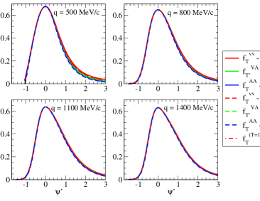
Figure 1: Transverse RMF scaling functions normalized to the maximum value corresponding to an arbitrary reference function and relocated at $\psi^{\prime}=0$ (see text for details). The convention used to label the different curves is as follows: “$e$” for electron-induced reactions and “$\nu$” (“a$\nu$”) for neutrino- (antineutrino-) induced reactions.

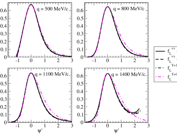
Figure 2: As in Fig. 1, but now for the longitudinal RMF scaling functions.

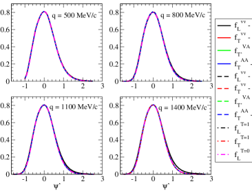
Figure 3: As in Fig. 1, but in this case the results correspond to RPWIA. Transverse and longitudinal sets are presented together.

We do not present results of $f_{CC}^{AA}$, $f_{CL}^{AA}$, $f_{LL}^{AA}$ for neutrino and antineutrino scattering, and $f_{T}^{T=0}$ for electron scattering because they are very sensitive to small effects due to cancellations and/or to the smallness of the denominator ($G$ function) which appears in the definition of the scaling function (see Appendix A). The first three are seen to be insignificant for neutrino reactions, whereas the fourth does not enter in that case and is known to be a minor correction in the QE regime for electron scattering.

Results obtained within RPWIA show that all scaling functions have the same shape (see Fig. 3). This comment also applies to models based on nonrelativistic and semirelativistic descriptions (see Amaro05b ; Amaro07 ).

Within the RMF model, all transverse scaling functions approximately collapse in a single one. On the contrary, the longitudinal responses are grouped in two sets: one corresponding to the pure electron isovector and neutrino (antineutrino) VV-responses, i.e., $f_{L}^{T=1,ee^{\prime}}$ and $f_{L}^{VV,\nu(\bar{\nu})}$, and the other to the isoscalar contribution for electrons, namely, $f_{L}^{T=0,ee^{\prime}}$. This result emerges for all $q$-values and tends to be rather general. It is also noticeable that the tail is higher and more extended for the transverse responses, whereas for the longitudinal ones it tends to go down faster.

It is worth observing that in all cases the RMF scaling functions display a much more pronounced asymmetric shape than the RPWIA ones, an effect related to the specific treatment of final state interactions.

II.2 Height and position of the peak of the scaling function

In the top (bottom) panel in Fig. 4 the peak-height of the transverse (longitudinal) set of scaling functions is presented as function of $q$. The results correspond to RMF and RPWIA predictions. We observe that the peak-heights of the scaling functions within RPWIA are almost $q$-independent (and very close to RFG value of 3/4), while the RMF ones present a mild $q$-dependence in the transverse set and a somewhat stronger one for the longitudinal set. It is well known that FSI tend to decrease the peak-height of the responses putting the strength in the tails, especially at high energy loss. This is particularly true for the RMF approach Maieron03 ; Caballero06 and models based on the Relativistic Green Function (RGF) Meucci03 ; Meucci09 . Similar effects have also been observed within semirelativistic approaches Amaro05b ; Amaro07 . More specifically, in Fig. 4, we see that the discrepancies between the RMF and RPWIA peak-height results average to $\sim$25$\%$ in the transverse set. On the other hand, those discrepancies are more strongly $q$-dependent in the longitudinal sector, reaching $\sim$30$\%$ ($\sim$70$\%$) in the lower (higher) $q$-region for the longitudinal isovector responses (blue lines). Finally, the difference between the isoscalar longitudinal $(e,e^{\prime})$ scaling function produced by RMF and RPWIA (magenta dashed-dotted lines) is somewhat smaller: $\sim$20$\%$ ($\sim$30$\%$) for lower (higher) $q$.

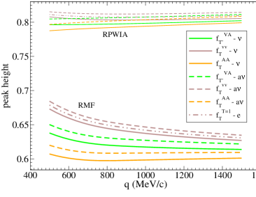
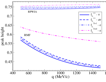
Figure 4: (Top panel) Peak height of the transverse set of scaling functions as a function of the transferred momentum $q$. The upper set of lines corresponds to the prediction within RPWIA (thin lines), while the lower set of lines has been obtained with the RMF model. (Bottom panel) As for the top panel, but now for the longitudinal set of scaling functions.

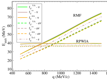
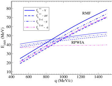
Figure 5: (Top panel) Shift energy, $E_{shift}$, needed in order to have the corresponding scaling function peak located at $\psi^{\prime}=0$, as function of $q$. Results for the transverse set of scaling functions. (Bottom panel) As for the top panel, but now for the longitudinal set of scaling functions.

In Fig. 5 we study the position of the peak of the transverse and longitudinal sets. To this scope we display the energy shift, $E_{shift}$, needed to place the peak of the scaling function at $\psi^{\prime}=0$ as a function of $q$. In the top panel of Fig. 5 we see that for the RPWIA transverse scaling function, $E_{shift}$ is almost $q$-independent, while the corresponding RMF shift increases almost linearly with the momentum transfer. This $q$-linear dependence of $E_{shift}$ was already observed and discussed within the framework of a semirelativistic model based on the use of the Dirac-equation-based potential Amaro07 . Approximately the same behavior is observed for the longitudinal set (bottom panel in Fig. 5), although in this case the RPWIA results are softly linearly dependent on $q$. It is also worth mentioning that the three transverse scaling functions linked to the same neutrino or antineutrino process, $f_{T}^{VV}$, $f_{T}^{AA}$ and $f_{T^{\prime}}^{VA}$, collapse in a single line for RMF as for RPWIA.

From the analysis of Figs. 4 and 5 one may conclude that $f_{L}^{T=1,ee^{\prime}}$ presents the same behavior (height and position) as $f_{L}^{VV,\nu(\bar{\nu})}$ (blue lines). The differences between these three curves are approximately constant and arise from the differences in the bound states involved in the reaction: proton+neutron in $(e,e^{\prime})$, neutron in $(\nu,\mu^{-})$ and proton in $(\bar{\nu},\mu^{+})$. The Coulomb-FSI, namely, the electromagnetic interaction between the struck nucleon and the residual nucleus, which plays a role when the outgoing nucleon is a proton, could also introduce a difference; however, we find that its effects are negligible and that the differences between, for instance, $f_{L}^{VV,\nu}$ and $f_{L}^{VV,\bar{\nu}}$ in RPWIA (where no Coulomb-FSI are involved) are almost the same as in RMF (see Figs. 4 and 5).

As mentioned in the Introduction, the strong $q$-dependence of the RMF peak position, which keeps growing with the momentum transfer, is a shortcoming of the model, whose validity is questionable at very high $q$. Indeed for high $q$ the outgoing nucleon carries a large kinetic energy so the effects of FSI should be suppressed for such kinematics. In fact, it would be desirable that the RMF results tend to approach the RPWIA ones for increasing momentum transfer, i.e., the scaling functions should become more symmetric, and a saturation of the peak-height reduction and of the energy shift should be observed. That trend is consistent with the scaling arguments Donnelly99a ; Maieron02 ; Caballero06 , i.e., the experimental evidence of a universal scaling function for increasing $q$. This is one of the motivations to use an alternative model if one aims to reproduce the experimental $(e,e^{\prime})$ data at medium-to-high momentum transfers.

A possible alternative for the behavior of the peak height, peak position and shape of the scaling functions would be to implement the RMF model at low to intermediate-$q$ and the RPWIA one for higher $q$-values.

II.3 Sum rules

In Fig. 6, the values of the integrals over $\psi^{\prime}$ of the different scaling functions within RMF model are presented versus $q$. These are given by

$$S_{i}(q)=\int_{-\infty}^{\infty}f_{i}(\psi,q)\,d\psi\,.$$ (10)

The integration limits, denoted by $(-\infty,+\infty)$, extend in reality to the range allowed by the kinematics. The above integral in the case of the longitudinal $(e,e^{\prime})$ scaling function was shown to coincide, apart from some minor discrepancies ascribed to the particular single-nucleon expressions considered and the influence of the nuclear scale introduced, with the results obtained using the standard expression for the Coulomb Sum Rule (see Caballero10a for details). Hence in what follows we denote the functions $S_{i}(q)$ simply as sum rules.

We see that all integrals of the transverse set are above unity and increase almost linearly with $q$. On the contrary, the integrals of $f_{L}^{VV,\nu(\bar{\nu})}$ and $f_{L}^{T=1,ee^{\prime}}$ (blue lines) are below unity and decrease with $q$ up to $q=1100$ MeV/c. From $q=900$ MeV/c they begin to be stable around the value $0.7$. Then, from $q=1200$ MeV/c to higher $q$-values the integrals start growing again. However, notice that in that $q$-region the result of the integrals is very sensitive to the behavior of the tail of these particular scaling functions (see Fig. 2). Finally, the values of the integral of the longitudinal isoscalar function, $f_{L}^{T=0,ee^{\prime}}$, is approximately constant and close to unity. The behavior of the integrals of the two longitudinal scaling functions for $(e,e^{\prime})$ is consistent with the analysis of the Coulomb sum rule for these two models (see Caballero10a ).

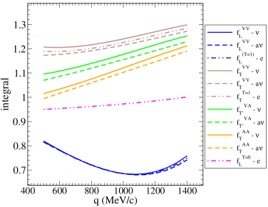
Figure 6: Integrals of RMF scaling functions as functions of $q$.

Although not shown here, we have also studied the integrals within RPWIA. In general, one observes that they are almost $q$-independent in all cases: $\sim$1 for the longitudinal set and $\sim$1.05 for the transverse set.

III Extension of the SuperScaling Approach: the SuSAv2 model

In this section we build the SuSAv2 model as a combination of the original SuSA model and some of the physical ingredients contained in the RMF and RPWIA models.

On the one hand, as we have shown in the previous sections, the RMF model has a $q$-dependence that is too strong. On the other hand, the SuSA model does not account for the difference between the longitudinal and transverse $(e,e^{\prime})$ scaling functions. Similarly, SuSA does not account for possible differences in the scaling function linked to isospin effects (isovector, isoscalar, isovector+isoscalar) or to the character of the current ($J_{V}J_{V}$: vector-vector, $J_{V}J_{A}$: axial-vector, $J_{A}J_{A}$: axial-axial).

Thus, we aim to improve the SuSA model by introducing into it specific information from the RMF approach. The goal is to get a new version of SuSA, SuSAv2. The model is based on the following four assumptions:

1. $f_{L}^{ee^{\prime}}$ superscales, i.e, it is independent of the momentum transfer (scaling of first kind) and of the nuclear species (scaling of second kind). It has been proven that $f_{L}^{ee^{\prime}}$ superscales for a range of $q$ relatively low ($300<q<570$ MeV/c), see Donnelly99a . As in the original SuSA model, here we assume that superscaling is fulfilled by Nature.

2. $f_{T}^{ee^{\prime}}$ superscales. It has been shown that $f_{T}^{ee^{\prime}}$ approximately superscales in the region $\psi<0$ for a wide range of $q$ ($400<q<4000$ MeV/c), see Maieron02 . However we assume that once the contributions from non-QE processes are removed (MEC, $\Delta$-resonance, DIS, etc.) the superscaling behaviour could be extended to the whole range of $\psi$.

3. The RMF model reproduces quite well the relationships between all scaling functions in the whole range of $q$. This assumption is supported by the fact that RMF model is able to reproduce the experimental scaling function, $f_{L,\text{exp}}^{ee^{\prime}}$, and the fact that it naturally yields the inequality $f_{T}^{ee^{\prime}}>f_{L}^{ee^{\prime}}$.

4. At very high $q$ the effects of FSI disappear and all scaling functions must approach the RPWIA results.

Contrary to what is assumed in the SuSA model, where only $f_{L,\text{exp}}^{ee^{\prime}}$ is used as reference scaling function to build all nuclear responses, within SuSAv2 we use three RMF-based reference scaling functions (which will be indicated with the symbol $\tilde{f}$): one for the transverse set, one for the longitudinal isovector set and another one to describe the longitudinal isoscalar scaling function in electron scattering. This is consistent with the study of the shape of the scaling functions discussed in the previous section, where three different sets of scaling functions emerged.

We employ the experimental scaling function $f_{L,\text{exp}}^{ee^{\prime}}$ as guide in our choices for the reference ones. In Fig. 7 we display the RMF longitudinal scaling function, $f_{L}$, for several representative values of $q$. Notice that the functions have been relocated by introducing an energy shift (see later) so that the maximum is at $\psi^{\prime}=0$. It appears that scaling of first kind is not perfect and some $q$-dependence is observed. Although all the curves are roughly compatible with the experimental error bars, the scaling function that produces the best fit to the data corresponds to $q\approx 650$ MeV/c. This is the result of a $\chi^{2}$-fit to the 25 experimental data of $f^{ee^{\prime}}_{L,exp}$, as illustrated in the inner plot in Fig. 7.

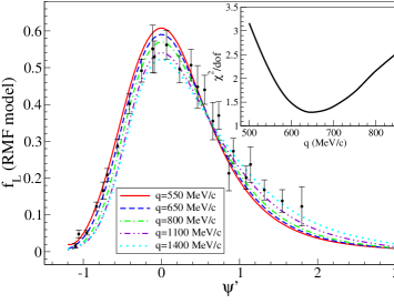
Figure 7: Longitudinal scaling function for $(e,e^{\prime})$ computed within RMF. The scaling functions have been shifted to place the maximum at $\psi^{\prime}=0$. In the inner smaller plot the reduced-$\chi^{2}$, defined as $\chi^{2}/25=\frac{1}{25}\sum_{i=1}^{25}[(f^{ee^{\prime}}_{L,exp,i}-f_{L,i}^{RMF})/\sigma_{L,i}^{exp}]^{2}$ where $\sigma_{L,i}^{exp}$ are the errors of the experimental data, is presented versus $q$. The minimum $\chi^{2}$ is around $q=650$ MeV/c. Data from Ref. Jourdan96 .

According to this result, we identify the reference scaling functions with $f^{T=1,ee^{\prime}}_{L}$, $f^{T=0,ee^{\prime}}_{L}$ and $f^{T=1,ee^{\prime}}_{T}$ evaluated within the RMF model at $q=650$ MeV/c and relocated so that the maximum is at $\psi^{\prime}=0$ (we will account for the energy shift later):

$$\tilde{f}_{T} \equiv f_{T}^{T=1,ee^{\prime}}|^{RMF}_{q=650}$$ (11)

$$\tilde{f}_{L,T=1} \equiv f_{L}^{T=1,ee^{\prime}}|^{RMF}_{q=650}$$ (12)

$$\tilde{f}_{L,T=0} \equiv f_{L}^{T=0,ee^{\prime}}|^{RMF}_{q=650}\,.$$ (13)

Thus, by construction, the $(e,e^{\prime})$ longitudinal scaling function built within SuSAv2 is $f_{L}|^{SuSAv2}=f_{L}|^{RMF}_{q=650}\approx f_{L,exp}^{ee^{\prime}}$. In order to work with these reference scaling functions we need analytical expressions for them. To that end, we have used a skewed-Gumbel function which depends on four parameters. The expressions that parametrize the reference scaling functions are presented in Appendix B.

The next step before building the responses (see Eqs. (2-9)) is to define the rest of scaling functions starting from the reference ones. According to the third assumption for the construction of SuSAv2, we define:

$$f_{L}^{VV,\nu(\bar{\nu})}(q)=\mu_{L}^{VV,\nu(\bar{\nu})}(q)\tilde{f}_{L,T=1}$$ (14)

$$f_{T}^{VV,\nu(\bar{\nu})}(q)=\mu_{T}^{VV,\nu(\bar{\nu})}(q)\tilde{f}_{T}$$ (15)

$$f_{T}^{AA,\nu(\bar{\nu})}(q)=\mu_{T}^{AA,\nu(\bar{\nu})}(q)\tilde{f}_{T}$$ (16)

$$f_{T^{\prime}}^{VA,\nu(\bar{\nu})}(q)=\mu_{T}^{VA,\nu(\bar{\nu})}(q)\tilde{f}_{T}\,,$$ (17)

where we have introduced the ratios $\mu$ defined as:

$$\mu_{T}^{VV,\nu(\bar{\nu})}(q) \equiv f_{T}^{VV,\nu(\bar{\nu})}(q)/f_{T}^{T=1,ee^{\prime}}(q)$$ (18)

$$\mu_{T}^{AA,\nu(\bar{\nu})}(q) \equiv f_{T}^{AA,\nu(\bar{\nu})}(q)/f_{T}^{T=1,ee^{\prime}}(q)$$ (19)

$$\mu_{T^{\prime}}^{VA,\nu(\bar{\nu})}(q) \equiv f_{T^{\prime}}^{\nu(\bar{\nu})}(q)/f_{T}^{T=1,ee^{\prime}}(q)\,,$$ (20)

for the transverse set and

$$\mu_{L}^{VV,\nu(\bar{\nu})}(q)\equiv f_{L}^{VV,\nu(\bar{\nu})}(q)/f_{L}^{T=1,ee^{\prime}}(q)\,,$$ (21)

for the longitudinal one.

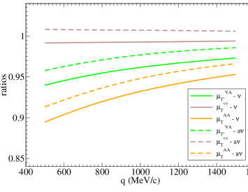
Figure 8: Ratios of transverse scaling functions.

From the results of these ratios, presented in Fig. 8, it emerges that one can assume $\mu_{T}^{VV,\nu(\bar{\nu})}(q)\approx 1$, with an error of the order of $\sim$1$\%$. The same assumption could be made for $\mu_{T^{\prime}}^{\nu(\bar{\nu})}(q)$ and $\mu_{T}^{AA,\nu(\bar{\nu})}(q)$ but in this case the error averages to $\sim$3$\%$ and $\sim$7$\%$, respectively. Regarding the longitudinal isovector set, although not shown, one gets $\mu_{L}^{VV,\nu(\bar{\nu})}\approx 1$ with an error of the order $\sim$1$\%$.

Therefore it is a good approximation to set all of the $\mu$-ratios equal to unity in Eqs. (14,15,16,17).

In summary, within SuSAv2 we will assume: $f_{T}^{VV,\nu(\bar{\nu})}=f_{T}^{AA,\nu(\bar{\nu})}=f_{T^{\prime}}^{VA,\nu(\bar{\nu})}=\tilde{f}_{T}$ and $f_{L}^{VV,\nu(\bar{\nu})}=\tilde{f}_{L}$. Notice that since $f_{T}^{T=0,ee^{\prime}}$ and $f_{CC,CL,LL}^{AA,\nu(\bar{\nu})}$ are not defined (see Sect. II.1) we will also assume $f_{T}^{T=0,ee^{\prime}}=\tilde{f}_{L,T=1}$ and $f_{CC,CL,LL}^{AA,\nu(\bar{\nu})}=\tilde{f}_{L,T=1}$.

Finally, in order to implement the assumption number 4 of the model, namely the disappearance of FSI at high $q$, we build the SuSAv2 L and T scaling functions as linear combinations of the RMF-based and RPWIA reference scaling functions:

$${\cal F}_{L}^{T=0,1} \equiv \cos^{2}\chi(q)\tilde{f}_{L}^{T=0,1}+\sin^{2}\chi(q)\tilde{f}_{L}^{RPWIA}$$

$${\cal F}_{T} \equiv \cos^{2}\chi(q)\tilde{f}_{T}+\sin^{2}\chi(q)\tilde{f}_{T}^{RPWIA}\,,$$

where $\chi(q)$ is a $q$-dependent angle given by

$$\chi(q)\equiv\frac{\pi}{2}(1-[1+\exp{\left((q-q_{0})/w_{0}\right)}]^{-1})$$ (23)

with $q_{0}$=800 MeV/c and $w_{0}$=200 MeV. The reference RPWIA scaling functions, $\tilde{f}_{K}^{RPWIA}$, are evaluated at $q$=1100 MeV/c, while the reference RMF scaling functions, $\tilde{f}_{K}$, are evaluated at $q$=650 MeV/c (see discussion in Sect. II). The explicit parametrization of $\tilde{f}_{K}^{RPWIA}$ is given in Appendix B. With this procedure we get a description of the responses based on RMF behavior at lower-$q$ while for higher momentum transfers it mimics the RPWIA trend. The transition between RMF and RPWIA behaviors occurs at intermediate $q$-values, namely, $\sim q_{0}$, in a region of width $\sim w_{0}$.

The response functions (see Eqs. (2) and (4–9)) are simply built as:

$$R_{L}^{ee^{\prime}}(q,\omega) = \frac{1}{k_{F}}\left[{\cal F}_{L,T=1}(\psi^{\prime})G_{L}^{T=1}(q,\omega)\right.$$ (24)

$$+ \left.{\cal F}_{L,T=0}(\psi^{\prime})G_{L}^{T=0}(q,\omega)\right]$$

$$R_{T}^{ee^{\prime}}(q,\omega) = \frac{1}{k_{F}}{\cal F}_{T}(\psi^{\prime})\left[G_{T}^{T=1}(q,\omega)\right.$$ (25)

$$+ \left.G_{T}^{T=0}(q,\omega)\right]$$

$$R_{L}^{VV,\nu(\bar{\nu})}(q,\omega)=\frac{1}{k_{F}}{\cal F}_{L,T=1}(\psi^{\prime})G_{L}^{VV}(q,\omega)$$ (26)

$$R_{CC}^{AA,\nu(\bar{\nu})}(q,\omega)=\frac{1}{k_{F}}{\cal F}_{L,T=1}(\psi^{\prime})G_{CC}^{AA}(q,\omega)$$ (27)

$$R_{CL}^{AA,\nu(\bar{\nu})}(q,\omega)=\frac{1}{k_{F}}{\cal F}_{L,T=1}(\psi^{\prime})G_{CL}^{AA}(q,\omega)$$ (28)

$$R_{LL}^{AA,\nu(\bar{\nu})}(q,\omega)=\frac{1}{k_{F}}{\cal F}_{L,T=1}(\psi^{\prime})G_{LL}^{AA}(q,\omega)$$ (29)

$$R_{T}^{\nu(\bar{\nu})}(q,\omega) = \frac{1}{k_{F}}{\cal F}_{T}(\psi^{\prime})\left[G_{T}^{VV}(q,\omega)\right.$$ (30)

$$+ \left.G_{T}^{AA}(q,\omega)\right]$$

$$R_{T^{\prime}}^{\nu(\bar{\nu})}(q,\omega) = \frac{1}{k_{F}}{\cal F}_{T}(\psi^{\prime})G_{T^{\prime}}^{VA}(q,\omega).$$ (31)

Furthermore, in order to reproduce the peak position of RMF and RPWIA scaling functions, discussed in Sect. II.2, within SuSAv2 we consider a $q$-dependent energy shift, namely, $E_{shift}(q)$. This quantity modifies the scaling variable $\psi(q,\omega)\longrightarrow\psi^{\prime}(q,\omega,E_{shift})$ as described in Appendix A. In particular, we build this function $E_{shift}(q)$ from the results of the RMF and RPWIA models presented in Fig. 5. Thus, $E_{shift}(q)$ for the reference RMF scaling function $\tilde{f}_{T}[\psi^{\prime}(E_{shift})]$ is the parametrization of the brown dot-dot-dashed line in the top panel of Fig. 5. The same procedure is used to parametrize $E_{shift}(q)$ corresponding to the $\tilde{f}_{L,T=1}$ and $\tilde{f}_{L,T=0}$, but in this case using, as an average, the blue dot-dot-dashed line from the bottom panel of Fig. 5. Moreover, for the RPWIA case we use for the longitudinal and transverse responses the corresponding RPWIA $E_{shift}(q)$ curves shown in Fig. 5.

Notice that for $q\lesssim 300-350$ MeV/c it is difficult to extract the peak position of the RMF scaling function from the data so we have set a minimum shift energy, $E_{shift}=10$ MeV. This choice of $E_{shift}(q)$ depending on the particular $q$-domain region considered is solely based on the behavior of the experimental cross sections and their comparison with our theoretical predictions (see results in next sections). In the past we have considered a fixed value of $E_{shift}$ (different for each nucleus) to be included within the SuSA model in order to fit the position of the QE peak for some specific $q$-intermediate values. Here we extend the analysis to very different kinematics covering from low to much higher $q$-values. On the other hand, the RMF model leads the cross section to be shifted to higher values of the transferred energy. This shift becomes increasing larger for higher $q$-values as a consequence of the strong, energy-independent, highly repulsive potentials involved in the RMF model. Comparison with data (see the results in the next sections) shows that the shift produced by RMF is too large. Moreover, at very high $q$-values, one expects FSI effects to be less important and lead to results that are more similar to those obtained within the RPWIA approach. This is the case when FSI are described through energy-dependent optical potentials. Therefore, as already mentioned, our choice for the functional dependence of $E_{shift}(q)$ is motivated as a compromise between the predictions of our models and the comparisons with data.

IV Comparison with electron scattering data

In this section we present a systematic comparison of total inclusive ¹²C$(e,e^{\prime})$ experimental cross sections and the predictions for the QE process within RMF, SuSA and SuSAv2 models. As mentioned, data correspond to the total inclusive cross section which includes contributions from several channels, mainly: QE scattering, inelastic scattering, many-nucleon emission, etc. The models presented in this work aim to describe only the QE process. Therefore, one expects that the models do not reproduce the total inclusive experimental data corresponding to kinematical situations in which non-QE contributions play some role. Thus, the main interest of the systematic analysis presented in this section is the comparison between SuSAv2 predictions and those from the SuSA and RMF models. Full analyses of the inclusive $(e,e^{\prime})$ cross section (including descriptions of QE and non-QE contributions) have been presented with some success in the past Barbaro04 ; Amaro05a ; Maieron09 . We plan to complete the description of the inclusive process within the context of SuSAv2 model, as was made in Amaro05a ; Maieron09 within SuSA, in a near future.

In Figs. 9-11 we present the comparison of the $(e,e^{\prime})$ experimental data and models. Due to the large amount of available data on ¹²C$(e,e^{\prime})$ at different kinematics (see ee-data ; Benhar:2006wy ) in these three figures we only show some representative examples. Each figure is labeled by the incident electron energy, $\varepsilon_{i}$ (in MeV), the scattering angle, $\theta_{e}$, and the transferred momentum corresponding to the center of the quasielastic peak, $q$ (in MeV/c). Pauli Blocking has been included in the SuSA and SuSAv2 models following the procedure described in Rosenfelder:1980nd ; Megias14 . In Appendix C we present a comparison of the models (SuSA and SuSAv2) and data when PB is or is not included. The panels in Figs. 9-11 are organized according to the value of the transferred momentum (at the center of the QE peak) in three sets: low-$q$ (from $q=238$ to $q=333$ MeV/c) in Fig. 9, medium-$q$ (from $q=401$ to $q=792$ MeV/c) in Fig. 10 and, high-$q$ (from $q=917$ to $q=3457$ MeV/c) in Fig. 11. The only phenomenological parameters entering in the calculation are the Fermi momentum $k_{F}$ and the energy shift $E_{shift}$. For these we use $k_{F}=228$ MeV/c (see Maieron02 ) in both SuSA and SuSAv2 models. A constant energy shift of 20 MeV is employed in SuSA Maieron02 while a $q$-dependent function, the one described in Sect. III, is used for $E_{shift}$ in the SuSAv2 model.

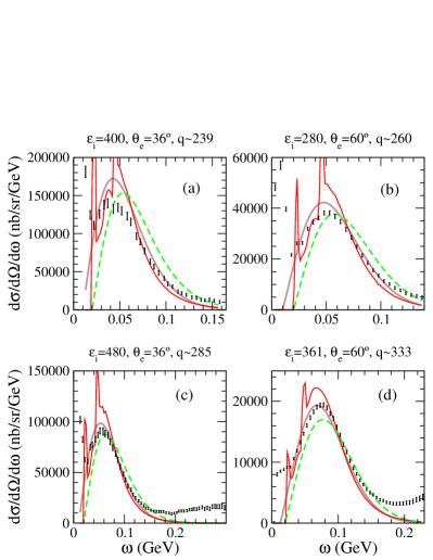
Figure 9: Comparison of inclusive ¹²C$(e,e^{\prime})$ cross sections and predictions of the RMF (red), SuSA (green-dashed) and SuSAv2 (brown) models (see text for details). Set of panels corresponding to low-$q$ values. Data taken from ee-data .

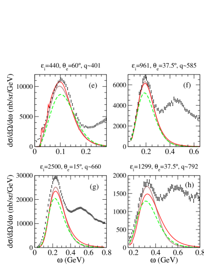
Figure 10: Continuation of Fig. 9. Set of panels corresponding to medium-$q$ values.

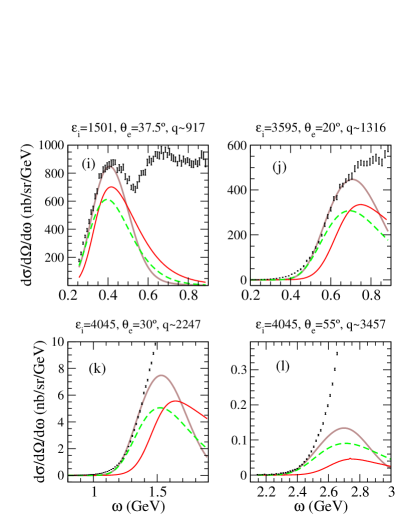
Figure 11: Continuation of Fig. 9. Set of panels corresponding to high-$q$ values.

We begin commenting on the low-$q$ panels presented in Fig. 9. The main contributions to the cross section from non-QE processes such as inelastic processes contributions ($\Delta$-resonance) and MEC, are very small, even negligible, in this low-$q$ region. In spite of that, when the transferred energy is small ($\omega\lesssim 50-60$ MeV) other processes such as collective effects contribute to the cross section making questionable the treatment of the scattering process in terms of IA-based models. This could explain, in part, the general disagreement between models and data in that $\omega$ region in (a), (b) and (c) panels.

Some clarifications are called for regarding the RMF results in Fig. 9, where sharp resonances appear at very low $\omega$ values. These correspond to 1p1h excitations with the phase shift of a given partial wave going through 90 degrees. With more complicated many-body descriptions these sharp features are smeared out.

In summary, in order to test the goodness of the models in the kinematical situation of Fig. 9, one should focus on the study of the tails of the cross sections where large enough $\omega$-values ($\omega\gtrsim 50-60$ MeV) are involved. There, one observes that SuSA predictions are clearly over-shifted to high $\omega$-values while RMF and SuSAv2 models fit the data reasonably well. In addition, as expected, SuSA results are systematically below SuSAv2 and RMF ones at the QEP.

We now discuss the results for medium-$q$ values presented in Fig. 10. First of all, one should mention that for the kinematics of this figure, in addition to the QE process, non-QE contributions are essential to describe the experimental cross sections. For instance, in panels (f), (g) and (h) the $\Delta$-peak appears clearly defined at $\omega$ values above the QE peak. In panel (e) one sees that in the region around the center of the QE-peak, the RMF prediction is above the SuSAv2 one, being closer to the experimental data. This is consistent with the behavior of the RMF scaling function studied in Sect. II (see Fig. 4), namely, the peak-height of the RMF scaling functions increases for decreasing $q$-values.

If the main non-QE contributions are not included in the modeling it is hard to conclude which model is better to reproduce the purely QE cross section. However, it seems reasonable to conclude that SuSAv2 improves the agreement with data compared to SuSA. For instance, in the situation of panel (e), it would be needed that non-QE processes would contribute more than 20% to the total cross section in order to SuSA fits the height of the data around the center of the QE-peak. A 20% fraction of the cross section linked to $\Delta$-resonance and MEC contributions is probably too much for that kinematics. Similar comments and conclusions apply to the results in panel (d) of Fig. 9.

For $q$-values close to $650$ MeV/c (panels (f) and (g)) RMF and SuSAv2 produce very similar results because of the way in which SuSAv2 has been defined (see Sect. III). For higher $q$-values, $q\gtrsim 792$ MeV/c ((h) panel), SuSAv2 and RMF predictions begin to depart from each other. In particular, RMF results tend to shift the peak to higher $\omega$ values and to place more strength in the tail while SuSAv2 cross sections tend to be more symmetrical due to the increasing dominance of the RPWIA scaling behavior (see Sect. III).

This difference is more evident for higher $q$-values, as observed in panels (j)-(l) of Fig. 11. It is important to point out that for the kinematics presented in Fig. 11 the non-QE contributions are not only important but they become dominant in the cross sections. This is the case presented in panels (k) and (l) where the QE-peak is not even visible in the data.

We could summarize the main conclusions from the present comparison of models and data as follows:

• Regarding the enhancement of the transverse response, $R_{T}$, in SuSAv2 compared with SuSA: in the absence of modeling of non-QE contributions, the most clear indications that support the SuSAv2 assumptions arise from the comparison with data at kinematical situations in which non-QE effects are supposed to be small (panels (e) and (d) in Figs. 9 and 10, respectively).

• Regarding the energy shift study: within the SuSA model we have used a constant energy shift of 20 MeV/c. On the one hand, from the comparison with the low-$q$ set of experimental data, Fig. 9, one concludes that 20 MeV is a too large shift. On the other hand, the comparison with the high-$q$ set of data, Fig. 11, suggests that 20 MeV is probably too small. Then, one is led to conclude that a constant energy shift is not the best option to reproduce $(e,e^{\prime})$ data. These results support the idea of introducing a $q$-dependent energy shift such as we made in the SuSAv2 model. The theoretical justification of this assumption was already discussed in Sect. III.

V Comparison with neutrino and antineutrino data

In recent years a significant amount of charge-changing quasielastic (CCQE) neutrino and antineutrino cross section data have been presented in the literature. In this section, as in the previous one for the $(e,e^{\prime})$ process, we compare the results of SuSAv2 model with some selected samples from different experiments: MiniBooNE MiniBooNECC10 ; MiniBooNECC13 , Miner$\nu$a MINERVAnu13 ; MINERVAnub13 and NOMAD NOMAD09 . The SuSA predictions are also presented as reference.

MiniBooNE has measured CCQE cross sections that are higher than most predictions based on IA. The excess, at relatively low energy ($\langle E_{\nu}\rangle\sim 0.7$ GeV), observed in MiniBooNE cross sections has been interpreted as evidence that non-QE processes may play an important role at that kinematics AmaroMEC ; MartiniMEC ; NievesMEC . It is important to point out that in the experimental context of MiniBooNE, “quasielastic” events are defined as those from processes or channels containing no mesons in the final state. Thus, in principle, in addition to the purely QE process, which in this work refers exclusively to processes induced by one-body currents (IA), meson exchange current effects (induced by two-body or many-body currents) should also be taken into account for a proper interpretation of data.

In Fig. 12 and Fig. 13 the double differential $(\nu,\mu^{-})$ and $(\bar{\nu},\mu^{+})$ cross sections measured by the MiniBooNE Collaboration are compared with SuSAv2 (solid-blue line) and SuSA (dashed-red line) predictions. The top and bottom panels correspond to a muon scattering angle of $\sim$63^o and $\sim$32^o, respectively. As observed, the SuSAv2 cross section is significantly larger than SuSA one, although it still falls below the MiniBooNE data. Thus, there is still room for MEC contributions. In Ivanov13 the RMF model is compared with the same set of data as shown in Figs. 12 and 13. In general, one observes that RMF and SuSAv2 models produce almost identical results (as happened in $(e,e^{\prime})$ for intermediate $q$-values).

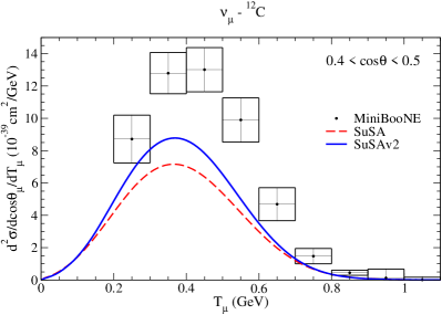
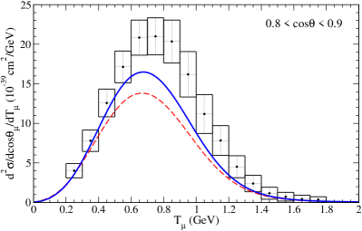
Figure 12: MiniBooNE double differential $(\nu,\mu^{-})$ cross section data MiniBooNECC10 are compared with SuSA (dashed-red line) and SuSAv2 (solid-blue line) predictions. In the top panel the scattering angle of the muon is $0.4<\cos\theta<0.5$, while in bottom panel $0.8<\cos\theta<0.9$.

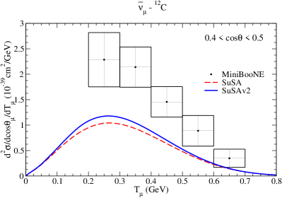
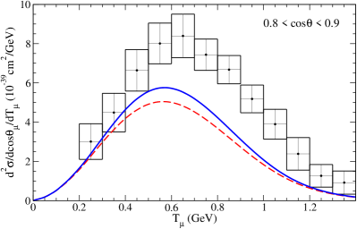
Figure 13: As in Fig. 12, but now for the antineutrino-induced reaction, $(\bar{\nu},\mu^{+})$. Data taken from MiniBooNECC13 .

In the NOMAD experiment the incident neutrino (antineutrino) beam energy is much larger, with a flux extending from $E_{\nu}$= 3 to 100 GeV. In this case, one finds that data are in reasonable agreement with predictions from IA models Megias13 ; Ivanov14 . Notice that the large error bars of these data do not allow for further definitive conclusions. In Fig. 14 we present the CCQE total cross section for neutrino (top panel) and antineutrino (bottom panel) reactions. Experimental data from NOMAD and MiniBooNE are compared with SuSA and SuSAv2. SuSAv2 improves the agreement with the NOMAD data, being, in general, closer to the center of the bins. The extension of the RMF model to very high energies requires at first complicated and very long time-consuming calculations. In this sense, the advantage of SuSAv2 is that it can be easily and rapidly extended up to very high neutrino energies. Although not shown here, preliminary results evaluated with the RMF model at NOMAD kinematics UdiasP are proved to be very similar to the SuSAv2 ones.

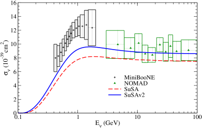
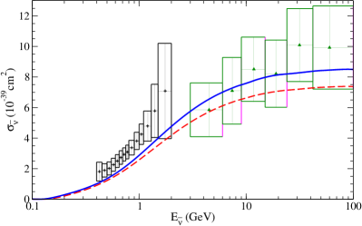
Figure 14: (Top panel) CCQE $(\nu,\mu^{-})$ cross section per nucleon is presented as a function of the incident neutrino energy, $E_{\nu}$. Data from MiniBooNE MiniBooNECC10 and NOMAD NOMAD09 are compared with SuSA (dashed-red line) and SuSAv2 (solid-blue line) predictions. (Bottom panel) As in top panel, but now for the antineutrino-induced reaction, ¹²C$(\bar{\nu},\mu^{+})$.

In the MINER$\nu$A experiment the neutrino energy flux extends from 1.5 to 10 GeV and is peaked at $E\nu\sim 3$ GeV, i.e., in between MiniBooNE and NOMAD energy ranges. Therefore, its analysis can provide useful information on the role played by meson-exchange currents in the nuclear dynamics. In recent work Megias14 it was found that, contrary to the comparison with the MiniBooNE data, the two IA models analyzed (RMF and SuSA) provide a good description of the MINER$\nu$A data without the need of significant contributions from MEC. In Fig. 15 we present the single-differential cross section ($d\sigma/dQ^{2}_{QE}$), measured by MINER$\nu$A, as a function of the reconstructed four-momentum transfer squared, $Q^{2}_{QE}$ (see MINERVAnu13 ; MINERVAnub13 for explicit definition of $Q^{2}_{QE}$). The SuSA and SuSAv2 results are compared with MINER$\nu$A data. In spite of the enhancement with respect to SuSA, SuSAv2 is not only consistent, but it also improves the agreement with MINER$\nu$A data. In fact, RMF and SuSAv2 models produce very close results (RMF predictions are presented in Megias14 ). Thus, contrary to the MiniBooNE situation, the comparison of MINER$\nu$A data and IA based models, in particular, RMF and SuSAv2, leaves little room for MEC contributions.

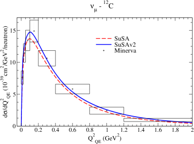
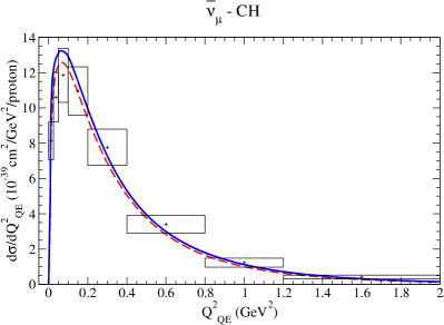
Figure 15: CCQE neutrino (upper panel) and antineutrino (lower panel) MINER$\nu$A data are compare with SuSA (dashed-red line) and SuSAv2 (solid-blue line) predictions. Data taken from MINERVAnu13 ; MINERVAnub13 .

A further general comment on the previous results is in order: the difference between SuSA and SuSAv2 is larger for neutrino than for antineutrino results. This occurs because of the cancellation occurring between $R_{T}$ (positive) and $R_{T^{\prime}}$ (negative) responses in antineutrino cross sections. Notice that the transverse responses are substantially enhanced in SuSAv2 compared with SuSA.

In summary we find that SuSAv2 compared with the SuSA model improves the comparison with neutrino and antineutrino data. Additionally, SuSAv2 (as SuSA) can easily make predictions at kinematics (very high energies) in which other more microscopic-based models, as RMF, require additional assumptions and demanding, time-consuming calculations.

VI Conclusions

The SuSA model, based on the scaling behavior exhibited by $(e,e^{\prime})$ data in the longitudinal channel, has been extensively used in the past not only to explain electron scattering, but also neutrino reactions. The basic idea of SuSA is the existence of a universal scaling function, the one ascribed to longitudinal $(e,e^{\prime})$ data, to be applied to any other process. Hence, SuSA makes use of the same scaling function for the two channels, longitudinal and transverse, involved in QE electron scattering reactions, as well as for the whole set of responses that enter in charged-current neutrino scattering processes.

On the other hand, the RMF model provides a description of the scattering reaction mechanism including the role played by FSI. The RMF model leads to a longitudinal scaling function in accordance with data, and hence, also in agreement with the SuSA result. However, contrary to the main assumption considered by SuSA, namely, the existence of only one universal scaling function, the RMF model provides a transverse scaling function that is higher by $\sim$20$\%$ compared with the longitudinal one. In other words, scaling of zeroth kind is not fulfilled by RMF. This result also seems to be in accordance with the preliminary analysis of data that shows the pure QE transverse channel to lead to a scaling function exceeding the longitudinal one by an amount, $\sim$20-25$\%$, similar to the one shown by the RMF results.

The analysis of neutrino reactions also introduces basic differences with the electron case. Whereas in the latter, responses contain isoscalar and isovector contributions, in the former, the responses are purely isovector. Moreover, not only pure vector-vector responses contribute to neutrino processes, but also axial-axial and the interference axial-vector one. All of these results, in addition to the preliminary analysis of the separate QE longitudinal and transverse responses, may introduce some doubts about the existence of a unique scaling function valid for all processes.

In this work we have pursued this problem and have extended the SuSA model by taking into account the results provided by the RMF approach. Hence we study in detail RMF scaling functions corresponding to all channels, and from this we select the minimum set of scaling functions, named reference scaling functions, that allow us to construct the cross section for electron and neutrino scattering reactions. The new model, called SuSAv2, takes care of the enhancement of the $(e,e^{\prime})$ transverse response compared with the longitudinal one, as well as the general behavior shown by the functions ascribed to neutrino reactions.

SuSAv2 is based on a “blend” between the properties of the RMF and RPWIA responses. The former appears to do well at low to intermediate values of the momentum transfer, for instance, yielding both an asymmetric scaling function and the T/L differences observed in electron scattering data. However, because of the strong energy independent scalar and vector potentials involved, the RMF model does less well at high values of $q$, where the energy shift is seen to be too strong and the high-energy tail in the RMF scaling function is likely too large. The RPWIA, on the other hand, does not work well at low to intermediate momentum transfers and, in fact, yields results that are not very different from those of the relativistic Fermi gas, which are known to be too symmetrical and not to contain the T/L differences seen in both the RMF results and in electron scattering data. What SuSAv2 attempts to do is to provide a cross-over from the low to intermediate momentum transfer regime (where the RMF results are employed) to the high-$q$ regime (where the results revert to those of the RPWIA). A particular, reasonable “blending” function has been used, although the specific parametrization assumed is not critical. Indeed, when updated 2p-2h MEC responses and updated representations of inelastic contributions are incorporated (see below) it will be appropriate to make detailed fits to existing electron scattering data and at that point one can refine the determination of the parameters used in this initial study.

We have applied the new SuSAv2 model to the description of electron and neutrino scattering, and have proved that SuSAv2 predictions are higher than the SuSA ones and are closer to data. This is so for electron scattering as well as for neutrino reactions. However, in the latter, theory still underestimates data in most of the cases, in particular, for the kinematics corresponding to the MiniBooNE experiment. This outcome is similar to the one already observed for the RMF results.

SuSAv2 model incorporates some basic ingredients not taken into account within SuSA, hence it clearly improves its reliability to the description of scattering processes, being at the same time a model that is easy to implement in the “generator codes” used to analyze the experiments. Moreover, its application to very high energies does not involve particularly demanding calculations in contrast to the RMF model that may can complex and long, time-consuming calculations.

Finally, a comment is in order concerning the ingredients incorporated by SuSAv2 (likewise for SuSA and RMF). This is a model based exclusively on the IA. Hence ingredients beyond the IA, i.e., two-body meson-exchange currents, inelastic contributions, etc., should be added to the model. Work along these lines is presently under way, as well as the application of SuSAv2 to different experimental kinematics: Argoneut, T2K, etc. These studies will be presented in a forthcoming publication.

This work was partially supported DGI (Spain): FIS2011-28738-C02-01, by the Junta de Andalucí a (FQM-170, 225), by the INFN National Project MANYBODY, and the Spanish Consolider-Ingenio 2000 programmed CPAN, in part (T. W. D.) by the U.S. Department of Energy under cooperative agreement DE-FC02-94ER40818 and in part (M. B. B.) by the INFN under project MANYBODY. G. D. M. acknowledges support from a fellowship from the Fundación Cámara (Universidad de Sevilla). R. G. J. acknowledges financial help from VPPI-US (Universidad de Sevilla). We thank J. M. Udías and M. V. Ivanov for fruitful discussions on the RMF calculations.

Appendix A Definition of the scaling functions

Within the context of the Relativistic Fermi Gas (RFG) model, the scaling variable is defined as (see Alberico88 ; Donnelly99a ; Donnelly99b )

$$\psi^{\prime}\equiv\frac{1}{\sqrt{\xi_{F}}}\frac{\lambda^{\prime}-\tau^{\prime}}{\sqrt{(1+\lambda^{\prime})\tau^{\prime}+\kappa\sqrt{\tau^{\prime}(\tau^{\prime}+1)}}}\,,$$ (32)

where $\xi_{F}=\sqrt{1+(k_{F}/M)^{2}}-1$, $\kappa=q/(2M)$, $\lambda^{\prime}=\omega^{\prime}/(2M)$ and $\tau=\kappa^{2}-\lambda^{\prime 2}$. $M$ is the nucleon mass and $k_{F}$ is the Fermi momentum Maieron02 . Additionally, we have introduced the variable $\omega^{\prime}=\omega-E_{shift}$. The quantity $E_{shift}$, which is different for each target nucleus Maieron02 , is introduced to account phenomenologically for the shift observed in the QE peak when the cross section is plotted as a function of $\omega$. Trivially, if $E_{shift}=0$ one recovers the unshifted scaling variable $\psi$.

A.1 Electromagnetic scaling functions

For $N=Z$ nuclei the isovector ($T=1$) and isoscalar ($T=0$) EM longitudinal, $L$, and transverse, $T$, scaling functions are:

$$f^{T=1,0}_{L,T}\equiv k_{F}\frac{R^{T=1,0}_{L,T}(\kappa,\lambda)}{G^{T=1,0}_{L,T}(\kappa,\lambda)}\,.$$ (33)

We have introduced the elementary cross sections

$$G^{T=1,0}_{L,T}(\kappa,\lambda)=\frac{1}{2\kappa{\cal D}}U^{T=1,0}_{L,T}(\kappa,\lambda)\,,$$ (34)

where

$$U^{T=1,0}_{L}(\kappa,\lambda)=\frac{\kappa^{2}}{\tau}\left[H^{T=1,0}_{E}+W^{T=1,0}_{2}\Delta\right]$$ (35)

$$U^{T=1,0}_{T}(\kappa,\lambda)=2\tau H^{T=1,0}_{M}+W^{T=1,0}_{2}\Delta\,,$$ (36)

with

$$H^{T=1,0}_{E,M} = \frac{Z+N}{4}(G_{E,M}^{T=1,0})^{2}$$ (37)

$$W^{T=1,0}_{2} = \frac{1}{1+\tau}\left[H^{T=1,0}_{E}+\tau H^{T=1,0}_{M}\right]\,.$$ (38)

$Z$ and $N$ are the number of protons and neutrons in the target nucleus, repectivaly. Finally,

$$\Delta \equiv \xi_{F}(1-\psi^{2})\left[\frac{\sqrt{\tau(\tau+1)}}{\kappa}+\frac{\xi_{F}}{3}\frac{\tau}{\kappa^{2}}(1-\psi^{2})\right]$$

$${\cal D} \equiv 1+\frac{1}{2}\xi_{F}(1+\psi^{2})\,.$$ (40)

Note that Pauli-blocking effects have been neglected here.

Notice that we have introduced the isoscalar and isovector EM form factors, $G_{E,M}^{T=1,0}$, which in terms of the more familiar proton and neutron ones are

$$G_{E,M}^{T=0}=G_{E,M}^{p}+G_{E,M}^{n}$$ (41)

$$G_{E,M}^{T=1}=G_{E,M}^{p}-G_{E,M}^{n}\,.$$ (42)

In this work, the GKex VMD-based model Lomon01 ; Lomon02 ; Crawford10 has been used for the proton and neutron EM form factors.

The total longitudinal, $L$, and transverse, $T$, scaling functions are defined as usual:

$$f_{L,T}\equiv k_{F}\frac{R_{L,T}(\kappa,\lambda)}{G_{L,T}(\kappa,\lambda)}\,,$$ (43)

where $G_{L,T}$ (and $U_{L,T}$) are built as above but with the following definition of $H_{E,M}$ and $W_{2}$:

$$H_{E,M} = Z(G_{E,M}^{p})^{2}+N(G_{E,M}^{n})^{2}$$ (44)

$$W_{2} = \frac{1}{1+\tau}\left[H_{E}+\tau H_{M}\right]\,.$$ (45)

A.2 Charge-changing neutrino and antineutrino scaling functions

In this case the current is purely isovector ($T=1$). As usual one defines

$$f^{\nu(\bar{\nu})}_{K}\equiv k_{F}\frac{R^{\nu(\bar{\nu})}_{K}(\kappa,\lambda)}{G_{K}(\kappa,\lambda)}\,,$$ (46)

where $K=L,T,CC,CL,LL,T^{\prime}$ for $VV$, $AA$ and $VA$ cases. The elementary cross sections are

$$G_{K}(\kappa,\lambda)=\frac{1}{2\kappa{\cal D}}U_{K}(\kappa,\lambda)\,,$$ (47)

which are defined in terms of

$$U_{L}^{VV} = \frac{\kappa^{2}}{\tau}\left[H_{E}^{T=1}+W_{2}^{T=1}\Delta\right]$$ (49)

$$U_{T}^{VV} = 2\tau H_{M}^{T=1}+W_{2}^{T=1}\Delta$$ (50)

$$U_{CC}^{AA} = \frac{\kappa^{2}}{\tau}\left[\left(\frac{\lambda}{\kappa}\right)^{2}H_{A}^{\prime}+H_{A}\Delta\right]$$ (51)

$$U_{LL}^{AA} = \frac{\kappa^{2}}{\tau}\left[H_{A}^{\prime}+\left(\frac{\lambda}{\kappa}\right)^{2}H_{A}\Delta\right]$$ (52)

$$U_{CL}^{AA} = -\frac{\kappa^{2}}{\tau}\left(\frac{\lambda}{\kappa}\right)\left[H_{A}^{\prime}+H_{A}\Delta\right]$$ (53)

$$U_{T}^{AA} = H_{A}\left[2(1+\tau)+\Delta\right]$$ (54)

$$U_{T^{\prime}}^{VA} = 2\sqrt{\tau(1+\tau)}H_{VA}\left[1+\Delta^{\prime}\right]\,.$$ (55)

The functions $H_{E,M}^{T=1}$ are given in Eq. (37) but in this case the factor $(Z+N)$ should be replaced by ${\cal N}$ which is $N$ or $Z$ for neutrino or antineutrino charge-changing reactions. We have also introduced the functions:

$$H_{A} = {\cal N}\left[G_{A}^{T=1}\right]^{2}$$ (56)

$$H_{A}^{\prime} = {\cal N}\left[G_{A}^{\prime}\right]^{2}$$ (57)

$$H_{VA} = {\cal N}G_{M}^{T=1}G_{A}^{T=1}$$ (58)

with

$$G_{A}^{\prime}\equiv G_{A}^{T=1}-\tau G_{P}^{T=1}=\frac{1}{1+|Q^{2}|/m_{\pi}^{2}}G_{A}^{T=1}\,.$$

and $G_{A}^{T=1}=g_{A}\left(1+|Q^{2}|/M_{A}^{2}\right)^{-2}$, being $g_{A}=1.2695$, $m_{\pi}$ the pion mass and $M_{A}=1.03$ GeV.

Finally, the quantity $\Delta^{\prime}$ which appears in Eq. (55) is defined as

$$\Delta^{\prime}=\frac{1}{\kappa\sqrt{1+1/\tau}}\frac{1}{2}\xi_{F}(1-\psi^{2})\,.$$ (60)

Note that Pauli-blocking effects have also been neglected here.

Appendix B Parameterization of the reference scaling functions

In this Appendix we summarize the parameterization of the reference scaling functions. The skewed-Gumbel (sG) function is

$$f_{sG}=S(\nu_{0};\psi)f_{G}(\psi_{0},\sigma,\beta;\psi)\,,$$ (61)

where

$$S(\nu_{0};\psi) = \frac{2}{1+e^{\nu/\nu_{0}}}$$ (62)

$$f_{G}(\psi_{0},\sigma,\beta;\psi) = \frac{\beta}{\sigma}e^{\nu}\exp[-e^{\nu}]$$ (63)

$$\nu = -\left(\frac{\psi-\psi_{0}}{\sigma}\right)\,.$$ (64)

In Table 1 are shown the values of the free parameters that fit the reference scaling functions $\tilde{f}_{L,T=1}$, $\tilde{f}_{L,T=0}$ and $\tilde{f}_{T}$. In Fig. 16 these reference scaling functions are presented as functions of the scaling variable $\psi$.

	$\tilde{f}_{L,T=1}$	$\tilde{f}_{L,T=0}$	$\tilde{f}_{T}$
$\beta$	$0.8923$	$1.0361$	$0.9425$
$\sigma$	$0.6572$	$0.5817$	$0.7573$
$\psi_{0}$	$0.1708$	$0.02217$	$-0.4675$
$1/\nu_{0}$	$-0.7501$	$-0.1163$	$2.9381$

Table 1: Values of the parameters that characterize the sG reference scaling functions.

The reference RPWIA scaling functions are

$$\tilde{f}_{L,T}^{RPWIA}=\frac{2(a_{3})_{L,T}}{1+\exp\left({\frac{\psi-a_{1}}{a_{2}}}\right)}\exp\left(-\frac{\left(\psi-a_{4}\right)^{2}}{a_{5}}\right)\,,$$ (65)

with $a_{1}=-0.892196$, $a_{2}=0.1792$, $(a_{3})_{L}=6070.85$, $(a_{3})_{T}=6475.57$, $a_{4}=1.74049$, $a_{5}=0.64559$.

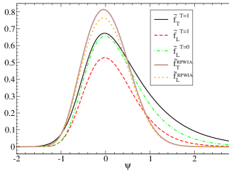
Figure 16: Reference scaling functions in SuSAv2 model.

Appendix C Pauli Blocking in SuSA and SuSAv2

In this Appendix we show the effects of Pauli Blocking (PB) in the SuSA and SuSAv2 models. The procedure employed to introduce PB in the SuSA model was already presented in Megias14 . The method, proposed in Rosenfelder:1980nd , consists in building a new scaling function by subtracting from the original one, $f[\psi(\omega,q)]$, its “mirror” function, $f[\psi(-\omega,q)]$ (see Megias14 for details). In the RFG this procedure yields exactly the same result as the usual way of introducing Pauli blocking via theta-functions. However the method can also be applied to models, like SuSA, which are not built starting from a momentum distribution. The same procedure is used in this work to introduce PB in SuSAv2 model.

We comment on Fig. 17 where SuSA results with and without PB are compared with a few sets of data at the kinematics in which PB effects are significant, i.e., very low $q$. In order to fit the position of the peak better, in this case we have used a shift energy of 10 MeV in the SuSA model (compared with the 20 MeV used in Figs. 9-11. This makes the comparison with data easier and allows us to focus on PB effects, namely, the width and peak height of the cross sections. In general we conclude that the agreement between SuSA and data improves when PB is introduced. SuSA without PB (green-dashed) produces cross sections too wide, while SuSA with PB (brown) provides narrower cross sections in better agreement with data. This is particularly true for instance in panels $(1)$ and $(2)$ in Fig. 17. The same comments apply to Fig. 18 where SuSAv2 with and without PB is compared with the same set of low-$q$ data. The lowest energy transfer data, corresponding to the excitation of resonant and collective states, cannot be described by any of the present models.

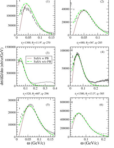
Figure 17: SuSA with and without Pauli Blocking is compared with data. $E_{shift}=10$ MeV has been employed.

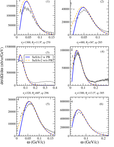
Figure 18: SuSAv2 with and without Pauli Blocking is compared with data.

A clear difference between SuSA and SuSAv2 (Figs. 17 and 18) is that the latter clearly overestimates the data in the region below and close to the peak. However, in all cases the maximum is placed at the region $\omega\lesssim 50-60$ MeV where, as discussed in Sect. IV, the validity of the models based on IA is questionable and no definitive conclusions can be drawn based on comparison of model and data in this $\omega$-region.

References

- (1) G. B. West, Phys. Rep. 263, 18 (1975)
- (2) J. A. Caballero, M. B. Barbaro, A. N. Antonov, M. V. Ivanov, and T. W. Donnelly, Phys. Rev. C 81, 055502 (2010)
- (3) A. N. Antonov, M. V. Ivanov, J. A. Caballero, M. B. Barbaro, J. M. Udias, E. Moya de Guerra, and T. W. Donnelly, Phys. Rev. C 83, 045504 (2011)
- (4) T. W. Donnelly and I. Sick, Phys. Rev. Lett. 82, 3212 (1999)
- (5) T. W. Donnelly and I. Sick, Phys. Rev. C 60, 065502 (1999)
- (6) W. M. Alberico, A. Molinari, T. W. Donnelly, E. L. Kronenberg, and J. W. Van Orden, Phys. Rev. C 38, 1801 (1988)
- (7) C. Maieron, T. W. Donnelly, and I. Sick, Phys. Rev. C 65, 025502 (2002)
- (8) D. B. Day, J. S. McCarthy, T. W. Donnelly, and I. Sick, Annu. Rev. Nucl. Part. Sci. 40, 357 (1990)
- (9) J. Jourdan, Nucl. Phys. A 603, 117 (1996)
- (10) C. Maieron, J. E. Amaro, M. B. Barbaro, J. A. Caballero, T. W. Donnelly, and C. F. Williamson, Phys. Rev. C 80, 035504 (2009)
- (11) J. E. Amaro, M. B. Barbaro, J. A. Caballero, T. W. Donnelly, A. Molinari, and I. Sick, Phys. Rev. C 71, 015501 (2005)
- (12) J. E. Amaro, M. B. Barbaro, J. A. Caballero, T. W. Donnelly, and C. Maieron, Phys. Rev. C 71, 065501 (2005)
- (13) J. A. Caballero, Phys. Rev. C 74, 015502 (2006)
- (14) J. A. Caballero, J. E. Amaro, M. B. Barbaro, T. W. Donnelly, C. Maieron, and J. M. Udías, Phys. Rev. Lett. 95, 252502 (2005)
- (15) J. A. Caballero, J. E. Amaro, M. B. Barbaro, T. W. Donnelly, and J. M. Udías, Phys. Lett. B 653, 366 (2007)
- (16) A. Meucci, J. A. Caballero, C. Giusti, F. D. Pacati, and J. M. Udías, Phys. Rev. C 80, 024605 (2009)
- (17) J. A. Caballero, M. C. Martínez, J. L. Herraíz, and J. M. Udías, Phys. Lett. B 688, 250 (2010)
- (18) J. E. Amaro, M. B. Barbaro, J. A. Caballero, T. W. Donnelly, and J. M. Udias, Phys. Rev. C 75, 034613 (2007)
- (19) C. Maieron, M. C. Martinez, J. A. Caballero, and J. M. Udias, Phys. Rev. C 68, 048501 (2003)
- (20) A. Meucci, F. Capuzzi, C. Giusti, and F. D. Pacati, Phys. Rev. C 67, 054601 (2003)
- (21) M. B. Barbaro, J. A. Caballero, T. W. Donnelly, and C. Maieron, Phys. Rev. C 69, 035502 (2004)
- (22) O. Benhar, D. Day, and I. Sick, arXiv:nucl-ex/0603032(Mar. 2006)
- (23) O. Benhar, D. Day, and I. Sick, Rev.Mod.Phys. 80, 189 (2008)
- (24) R. Rosenfelder, Annals Phys. 128, 188 (1980)
- (25) G. D. Megias, M. V. Ivanov, R. González-Jiménez, M. B. Barbaro, J. A. Caballero, T. W. Donnelly, and J. M. Udías, Phys. Rev. D 89, 093002 (2014)
- (26) A. A. Aguilar-Arevalo et al., Phys. Rev. D 81, 092005 (2010), [MiniBooNE Collaboration]
- (27) A. A. Aguilar-Arevalo et al., Phys. Rev. D 88, 032001 (2013), [MiniBooNE Collaboration]
- (28) G. A. Fiorentini et al., Phys. Rev. Lett. 111, 022502 (2013), [MINERA Collaboration]
- (29) L. Fields et al., Phys. Rev. Lett. 111, 022501 (2013), [MINERA Collaboration]
- (30) V. Lyubushkin et al., Eur. Phys. J. C 63, 355 (2009), [NOMAD Collaboration]
- (31) I. Ruiz-Simo, C. Albertus, J. E. Amaro, M. B. Barbaro, J. A. Caballero, and T. W. Donnelly, arXiv:1405.4280 [nucl-th](2014)
- (32) M. Martini, M. Ericson, G. Chanfray, and J. Marteau, Phys. Rev. C 81, 045502 (2010)
- (33) J. Nieves, I. Ruiz-Simo, and M. J. Vicente-Vacas, Phys. Lett. B 707, 72 (2012)
- (34) M. V. Ivanov, R. González-Jiménez, J. A. Caballero, M. B. Barbaro, T. W. Donnelly, and J. M. Udías, Phys. Lett. B 727, 265 (2013)
- (35) G. D. Megias, J. E. Amaro, M. B. Barbaro, J. A. Caballero, and T. W. Donnelly, Phys. Lett. B 725, 170 (2013)
- (36) M. V. Ivanov, A. N. Antonov, J. A. Caballero, G. D. Megias, et al., Phys. Rev. C 89, 014607 (2014)
- (37) J. M. Udias and M. V. Ivanov, Private communication (2013)
- (38) E. L. Lomon, Phys. Rev. C 64, 035204 (2001)
- (39) E. L. Lomon, Phys. Rev. C 66, 045501 (2002)
- (40) C. Crawford et al., Phys. Rev. C 82, 045211 (2010)