MPP–2014–314
LMU-ASC 48/14
CERN-PH-TH/2014-143
String Resonances at Hadron Colliders

Abstract

We consider extensions of the standard model based on open strings ending on D-branes, with gauge bosons due to strings attached to stacks of D-branes and chiral matter due to strings stretching between intersecting D-branes. Assuming that the fundamental string mass scale $M_{s}$ is in the TeV range and that the theory is weakly coupled, we discuss possible signals of string physics at the upcoming HL-LHC run (integrated luminosity $=3000\leavevmode\nobreak\ {\rm fb}^{-1}$) with a center-of-mass energy of $\sqrt{s}=14\leavevmode\nobreak\ {\rm TeV}$ and at potential future $pp$ colliders, HE-LHC and VLHC, operating at $\sqrt{s}=33$ and $100$ TeV, respectively (with the same integrated luminosity). In such D-brane constructions, the dominant contributions to full-fledged string amplitudes for all the common QCD parton subprocesses leading to dijets and $\gamma$ + jet are completely independent of the details of compactification and can be evaluated in a parameter-free manner. We make use of these amplitudes evaluated near the first $(n=1)$ and second $(n=2)$ resonant poles to determine the discovery potential for Regge excitations of the quark, the gluon, and the color singlet living on the QCD stack. We show that for string scales as large as 7.1 TeV (6.1 TeV), lowest massive Regge excitations are open to discovery at the $\geq 5\sigma$ in dijet ($\gamma$ + jet) HL-LHC data. We also show that for $n=1$ the dijet discovery potential at HE-LHC and VLHC exceedingly improves: up to 15 TeV and 41 TeV, respectively. To compute the signal-to-noise ratio for $n=2$ resonances, we first carry out a complete calculation of all relevant decay widths of the second massive-level string states (including decays into massless particles and a massive $n=1$ and a massless particle), where we rely on factorization and CFT techniques. Helicity wave functions of arbitrary higher spin massive bosons are also constructed. We demonstrate that for string scales $M_{s}\lesssim 10.5\leavevmode\nobreak\ {\rm TeV}$ ($M_{s}\lesssim 28\leavevmode\nobreak\ {\rm TeV}$) detection of $n=2$ Regge recurrences at HE-LHC (VLHC) would become the smoking gun for D-brane string compactifications. Our calculations have been performed using a semianalytic parton model approach which is cross checked against an original software package. The string event generator interfaces with HERWIG and Pythia through BlackMax. The source code is publically available in the hepforge repository.

1 Introduction

One of the most challenging problems in high-energy physics today is to find out what is the underlying theory that completes the standard model (SM). Despite its remarkable success, the SM is incomplete with many unsolved puzzles – the most striking one being the huge disparity between the strength of gravity and of the other three known fundamental interactions corresponding to the electromagnetic, weak, and strong nuclear forces. Indeed, gravitational interactions are suppressed by a very high-energy scale, the Planck mass $M_{\rm Pl}=G_{\rm N}^{-1/2}\sim 10^{19}\leavevmode\nobreak\ {\rm GeV}$, associated to a length $l_{\rm Pl}\sim 10^{-35}\leavevmode\nobreak\ {\rm m}$, where they are expected to become important. This hierarchy problem suggests that new physics could be at play above about the electroweak scale $M_{\rm EW}\sim G_{\rm F}^{-1/2}\sim 300\leavevmode\nobreak\ {\rm GeV}$ and has been arguably the driving force behind high-energy physics for several decades.

In a quantum theory, the hierarchy implies a severe fine-tuning of the fundamental parameters in more than 30 decimal places in order to keep the masses of elementary particles at their observed values. The reason is that quantum radiative corrections to all masses generated by the Higgs vacuum expectation value (VEV) are proportional to the ultraviolet cutoff which in the presence of gravity is fixed by the Planck mass. As a result, all masses are “attracted” to about $10^{16}$ times heavier than their observed values. A fine-tuned cancellation of the radiative corrections seems unnatural, even though it is in principle self-consistent. Naturalness implies that either the fundamental scale of gravity must be much smaller than the Planck mass, or else there should exist a mechanism which ensures this cancellation, perhaps arising from a new symmetry principle beyond the SM. Low-energy supersymmetry (SUSY) with all superparticle masses in the TeV region is a textbook example. Indeed, in the limit of exact SUSY, quadratically divergent corrections to the Higgs self-energy are exactly cancelled, while in the softly broken case, they are cutoff by the SUSY breaking mass splittings. On the other hand, for low-mass-scale strings, quadratic divergences are cutoff by the string scale $M_{s}$, and low-energy SUSY is not needed [1]. These two diametrically opposite viewpoints are experimentally testable at high-energy particle colliders, in particular at the CERN LHC.

The recent discovery of a particle with a mass around 126 GeV [2, 3], which seems to be the SM Higgs, has possibly plugged the final remaining experimental hole in the SM, cementing the theory further. The LHC data are so far compatible with the SM within 2$\sigma$ and its precision tests. It is also compatible with low-energy SUSY, although with some degree of fine-tuning in its minimal version. Indeed, in the minimal supersymmetric standard model (MSSM), the lightest Higgs scalar mass $m_{h}$ satisfies the inequality

$$m_{h}^{2}\lesssim m_{Z}^{2}\cos^{2}2\beta+\frac{3}{(4\pi)^{2}}\frac{m_{t}^{4}}{v^{2}}\left[\ln\frac{m_{\tilde{t}}^{2}}{m_{t}^{2}}+\frac{A^{2}_{t}}{m_{\tilde{t}}^{2}}\left(1-\frac{A_{t}^{2}}{12m_{\tilde{t}}^{2}}\right)\right]\lesssim(130\leavevmode\nobreak\ {\rm GeV})^{2}\,,$$ (1.1)

where the first term in the rhs corresponds to the tree-level prediction and the second term includes the one loop-corrections due to the top and stop loops. Here, $m_{Z}$, $m_{t}$, $m_{\tilde{t}}$ are the $Z$-boson and the top and stop quark masses, respectively; $v=\sqrt{v_{i}^{2}+v_{2}^{2}}$ with $v_{i}$ is the VEVs of the two Higgses; $\tan\beta=v_{2}/v_{1}$; and $A_{t}$ is the trilinear stop scalar coupling. Thus, a Higgs mass around 126 GeV requires a heavy stop $m_{t}\simeq 3\leavevmode\nobreak\ {\rm TeV}$ for vanishing $A_{t}$, or $A_{t}\simeq 3m_{\tilde{t}}\simeq 1.5\leavevmode\nobreak\ {\rm TeV}$ in the “best”-case scenario. These values are obviously consistent with the present LHC bounds on SUSY searches, but they are expected to be probed in the next run at double energy. Theoretically, they imply a fine-tuning of the electroweak scale at the percent to per mille level. This fine-tuning can be alleviated in supersymmetric models beyond the MSSM.

Low-mass-scale superstring theory provides a braneworld description of the SM, which is localized on membranes extending in $p+3$ spatial dimensions, the so-called D-branes. Gauge interactions emerge as excitations of open strings with endpoints attached on the D-branes, whereas gravitational interactions are described by closed strings that can propagate in all nine spatial dimensions of string theory [these comprise parallel dimensions extended along the $(p+3)$-branes and transverse dimensions]. For an illustration, consider type II string theory compactified on a six-dimensional torus $T^{6}$, which includes a D$p$-brane wrapped around $p-3$ dimensions of $T^{6}$ with the remaining dimensions along our familiar (uncompactified) three spatial dimensions. We denote the radii of the internal longitudinal directions (of the D$p$-brane) by $R_{i}^{\parallel}$, $i=1,\dots p-3$ and the radii of the transverse directions by $R^{\perp}_{j}$, $j=1,\dots 9-p$; see Fig. 1.

Figure 1: D-brane setup with $d_{\parallel}$ parallel and $d_{\perp}$ transverse internal directions.

The Planck mass, which is related to the string mass scale by

$$M_{\rm Pl}^{2}=\frac{8}{g_{s}^{2}}\ M_{s}^{8}\ \frac{V_{6}}{(2\pi)^{6}}\ ,$$ (1.2)

determines the strength of the gravitational interactions. Here,

$$V_{6}=(2\pi)^{6}\ \prod_{i=1}^{p-3}R^{\parallel}_{i}\ \prod_{j=1}^{9-p}R^{\perp}_{j}$$ (1.3)

is the volume of $T^{6}$ and $g_{s}$ is the string coupling. It follows that the string scale can be chosen hierarchically smaller than the Planck mass at the expense of introducing $9-p$ large transverse dimensions felt only by gravity, while keeping the string coupling small. For example, for a string mass scale $M_{s}\approx{\cal O}(1\leavevmode\nobreak\ {\rm TeV})$, the volume of the internal space needs to be as large as $V_{6}M_{s}^{6}\approx{\cal O}(10^{32}).$ On the other hand, the strength of coupling of the gauge theory living on the D-brane world volume is not enhanced as long as $R_{i}^{\parallel}\sim M_{s}^{-1}$ remain small,

$$\frac{1}{g^{2}}=\frac{1}{2\pi\,g_{s}}\ M_{s}{}^{p-3}\ \ \prod_{i=1}^{p-3}R_{i}^{\parallel}\ .$$ (1.4)

The weakness of the effective four-dimensional gravity compared to gauge interactions (ratio of $v/M_{\rm Pl}$) is then attributed to the largeness of the transverse space radii $R_{i}^{\perp}\sim 10^{32}l_{s}$ compared to the string length $l_{s}=M_{s}^{-1}$. Should nature be so cooperative, a whole tower of infinite string excitations will open up at this low-mass threshold, and new particles of spin $J$ follow the well-known Regge trajectories of vibrating strings: $J=J_{0}+\alpha^{\prime}M^{2}$, where $\alpha^{\prime}$ is the Regge slope parameter that determines the fundamental string mass scale

$$M_{s}={1\over\sqrt{\alpha^{\prime}}}\,.$$ (1.5)

Only one assumption will be necessary in order to set up a solid framework: the string coupling must be small for the validity of the above D-brane framework and of perturbation theory in the computation of scattering amplitudes. In this case, black hole production and other strong gravity effects occur at energies above the string scale; therefore, at least the lowest few Regge recurrences are available for examination, free from interference with some complex quantum gravitational phenomena.

In a series of publications, we have computed open string scattering amplitudes in D-brane models and have discussed the associated phenomenological aspects of low-mass string Regge recurrences related to experimental searches for physics beyond the SM [4, 5, 6, 7, 8, 9, 10, 11, 12, 13, 14, 15, 16]. We have shown that certain amplitudes to leading order in string coupling (but including all string $\alpha^{\prime}$ corrections) are universal [9, 10]. These amplitudes, which include $2\to 2$ scattering processes involving four gluons or two gluons and two quarks, are independent of the details of the compactification, such as the configuration of branes, the geometry of the extra dimensions, and whether SUSY is broken or not. This model independence makes it possible to compute the string corrections to $\gamma$ + jet and dijet signals at the LHC, which, if traced to low-mass-scale string theory, could with $100\leavevmode\nobreak\ {\rm fb}^{-1}$ of integrated luminosity (at $\sqrt{s}=14\leavevmode\nobreak\ {\rm TeV}$) probe deviations from SM physics at a $5\sigma$ significance for $M_{s}$ as large as 6.8 TeV [5, 8]. Indeed, the signal for string excitations is spectacularly dazzling: after operating for only a few months, with merely 2.9 inverse picobarns of integrated luminosity, the LHC7 CMS experiment ruled out $M_{s}<2.5\leavevmode\nobreak\ {\rm TeV}$ by searching for narrow resonances in the dijet mass spectrum [30]. In fact, the LHC has the capacity to discover strongly interacting narrow resonances in practically all ranges up to $\sqrt{s}_{\rm LHC}/2$, and therefore, since no significance excess above background has been observed thus far, the ATLAS [31] and CMS [32, 33] experiments have already excluded $M_{s}\lesssim 4.5\leavevmode\nobreak\ {\rm TeV}$.

In this work we extend our previous studies in various directions. In all our previous analyses, the discovery reach was laid out processing the string amplitudes using a semianalytic parton model approach. To confront technical detector challenges, however, the standard approach to data analysis is typically reliant on the existence of Monte Carlo event simulation tools that allow complete simulation of the signal. In this paper we are filling this gap by bringing the excitations of open strings into the ATLAS/CMS analysis software environment. A complete simulation with full Pythia treatment is quite a difficult task, because this event generator is set up in the same way perturbation theory works and consequently handles color flow lines of ordinary Feynman diagrams. Note that in string theory, there are processes (like $gg\to g\gamma$) that in ordinary field theory work only at loop level and their color lines do not follow the normal lines of tree-level Feynman diagrams. The proposed strategy here is to incorporate the string amplitudes into BlackMax [34, 35], a comprehensive black hole event generator for LHC analysis that interfaces (via the Les Houches accord [36]) to HERWIG and Pythia. The parton evolution and hadronization will then be performed with the correct format for direct implementation in the official Monte Carlo packages for simulating an actual experiment at the LHC. The two-step approach advanced herein can circumvent the color line technicalities and, at the same time, facilitate the comparison with high-multiplicity events from gravitational collapse.

Recently the idea of building a 33 TeV and/or 100 TeV circular proton-proton collider has gained momentum, starting with an endorsement in the Snowmass Energy Frontier report [37], and importantly followed by the creation of two parallel initiatives: one at CERN [38] and one in China [39]. In this paper we study the discovery reach and exclusion limits of lowest massive Regge excitations for the collider specifications,

Machine	$\sqrt{s}$ (TeV)	Final integrated luminosity
LHC phase I	$14$	$300$ fb-1
HL-LHC or LHC phase II	$14$	$3000$ fb-1
HE-LHC	$33$	$3000$ fb-1
VLHC	$100$	$3000$ fb-1

that are extensively discussed in the Snowmass Energy Frontier report [37]. For the HE-LHC and VLHC, the second excited string states may also be within reach. The decay widths of $n=2$ resonances into massless particles have been previously obtained in Refs. [22, 23]. For a full treatment, however, one still needs to compute the decay widths into one massive $n=1$ particle and a massless particle. Herein, we obatin all these widths by factorizing four-point amplitudes with one massive ($n=1$) and three massless particles.

The layout of the paper is as follows. We begin in Sec. 2 with an outline of the basic setting of intersecting D-brane models and we discuss general aspects of the effective low-energy theory inherited from properties of the overarching string theory. After that, we particularize the discussion to three- and four-stack intersecting D-brane configurations that realize the SM by open strings. For completness, in Sec. 3 we provide a summary of previous results. In particular, we give an overview of all formulae relevant for the $s$-channel string amplitudes of lowest massive Regge excitations leading to $\gamma$ + jet and dijets. Readers already familiar with these topics may skip this section. In Secs. 4 and 5 we present a complete calculation of all relevant decay widths of the second massive-level string states. The computation is performed in a model-independent and universal way, and so our results hold for all compactifications. Armed with the full-fledged string amplitudes of all partonic subprocesses, in Sec. 6 we quantify signal and background rates of $n=1$ and $n=2$ Regge recurrences in the early LHC phase I, HL-LHC, HE-LHC, and VLHC. In Sec. 7 we describe the input and output of the string event generator interface (SEGI) with HERWIG and Pythia through BlackMax and present some illustrative results. Finally in Sec. 8 we make a few observations on the consequences of the overall picture discussed herein.

A point worth noting at this juncture is that the tensor-to-scalar ratio ($r=0.20^{+0.07}_{-0.05}$) inferred from the excess B-mode power observed by the Background Imaging of Cosmic Extragalactic Polarization (BICEP2) experiment suggests in simple slow-roll models an era of inflation with energy densities of order $(10^{16}\leavevmode\nobreak\ {\rm GeV})^{4}$, not far below the Planck density [40]. This presumably suggests that low-mass-scale string compactifications in connection with large extra dimension are quite hard to realize. However, one should keep in mind that there is an ongoing controversy concerning the effect of background on the BICEP2 result [41, 42].

2 Intersecting D-brane string compactifications

D-brane low-mass-scale string compactifications provide a collection of building block rules that can be used to build up the SM or something very close to it [43, 44, 45, 46, 47, 48, 49, 50, 51, 52, 53, 54, 55, 56, 57]. The details of the D-brane construct depend a lot on whether we use oriented string or unoriented string models. The basic unit of gauge invariance for oriented string models is a $U(1)$ field, so that a stack of $N$ identical D-branes eventually generates a $U(N)$ theory with the associated $U(N)$ gauge group. In the presence of many D-brane types, the gauge group becomes a product form $\prod U(N_{i})$, where $N_{i}$ reflects the number of D-branes in each stack. Gauge bosons (and associated gauginos in a SUSY model) arise from strings terminating on one stack of D-branes, whereas chiral matter fields are obtained from strings stretching between two stacks. Each of the two strings end points carries a fundamental charge with respect to the stack of branes on which it terminates. Matter fields thus posses quantum numbers associated with a bifundamental representation. In orientifold brane configurations, which are necessary for tadpole cancellation, and thus consistency of the theory, open strings become in general nonoriented. For unoriented strings the above rules still apply, but we are allowed many more choices because the branes come in two different types. There are branes for which the images under the orientifold are different from themselves, and also branes that are their own images under the orientifold procedure. Stacks of the first type combine with their mirrors and give rise to $U(N)$ gauge groups, while stacks of the second type give rise to only $SO(N)$ or $Sp(N)$ gauge groups.

2.1 Mass mixing effect

In three-stack intersecting brane models, one could have one or two massive $U(1)$’s, depending on using $Sp(1)$ or $U(2)$ to realize $SU(2)$; while in four-stack models, one could have two or three massive $U(1)$’s. In general, one can have many $U(1)$’s in the intersecting brane model constructions including hidden sectors, and in these cases there will be many massive $U(1)$’s, which have been studied in Refs. [58, 59, 60]. Assuming no kinetic mixing, effectively the Lagrangian for all the $U(1)$’s from an $n$-stack model can be written as

$$\mathscr{L} =-\frac{1}{4}\sum_{a}F_{a}^{2}-\frac{1}{2}A_{a}M_{ab}^{2}A_{b}+\sum_{a}\bar{\psi}_{a}(i\not{\partial}+g^{\prime}_{a}Q_{a}\not{A}_{a})\psi_{a}\,,$$ (2.1)

where $\psi_{a}$ denotes the matter fields charged under $U(1)_{a}$ ($a,b,\cdots$ label the stack of D-branes), $g^{\prime}_{a}$ are the gauge couplings, and $Q_{a}$ are the charges. Note that the relation for $U(N)$ unification, $g^{\prime}_{a}=g_{a}/\sqrt{2N}$, holds only at $M_{s}$ because the $U(1)$ couplings ($g^{\prime}_{1},\,g^{\prime}_{2},\,g^{\prime}_{3},\,\cdots$) run differently from the non-Abelian $SU(3)$ ($g_{3}$) and $SU(2)$ ($g_{2}$) [61]. The $U(1)$ mass-squared matrix is of the form [62, 59]

$$M_{ab}^{2}=g^{\prime}_{a}g^{\prime}_{b}K_{ai}\mathcal{G}_{ij}K_{jb}^{T}\,,$$ (2.2)

where the integer-entry matrix $K$ contains all the information of local model constructions – wrapping numbers which give rise to correct family multiplicity and the (MS)SM spectrum – and $\mathcal{G}_{ij}$ is the metric of the complex structure moduli space. In general, the entries of the $U(1)$ mass-squared matrix are all of order of $M_{s}^{2}$. This $U(1)$ mass-squared matrix is positive semidefinite which has one zero eigenvalue that corresponds to the hypercharge. One could diagonalize $M_{ab}^{2}$ using an orthogonal matrix $O$ such that

$$O^{T}M^{2}O=\left(\begin{array}[]{ccccc}\lambda_{1}^{2}\\ &\lambda_{2}^{2}&&0\\ &&\ddots\\ &0&&\ddots\\ &&&&\lambda_{n}^{2}\end{array}\right)\equiv D^{2}\,,$$ (2.3)

where the eigenvalues are sorted from small to large, i.e., $\lambda_{i}<\lambda_{j}$ for $i<j$. $\lambda_{1}=0$ corresponds to the mass of the hypercharge gauge boson $Y_{\mu}\equiv A_{1,\mu}^{(m)}$. We can define the gauge boson corresponding to the lightest massive $U(1)$ to be $Z^{\prime}$. Here we only discuss the case that there is only one massless $U(1)$, and thus $D^{2}$ contains only one zero eigenvalue (hypercharge) and all other $U(1)$’s are massive. This transformation also takes the gauge fields from their original basis into the physical mass eigenbasis as (with an upper index ^(m))

$$A_{i}^{(m)}=\sum_{a}O_{ia}^{T}A_{a}\,.$$ (2.4)

The column vectors of the orthogonal matrix $O$ are the eigenvectors of $M^{2}$. Since the eigenvalues are already sorted, the first column vector gives rise to the hypercharge combination

$$Y_{\mu}=A_{1,\mu}^{(m)}=\sum_{a}O_{1a}^{T}A_{a}\,,$$ (2.5)

and the second column vector gives rise to

$$Z_{\mu}^{\prime}=A_{2,\mu}^{(m)}=\sum_{a}O_{2a}^{T}A_{a}\,,$$ (2.6)

and so on. Conversely, one could also write the gauge bosons in the original basis in terms of the mass eigenstates

$$A_{a}=\sum_{i}O_{ai}A_{i}^{(m)}\,.$$ (2.7)

After the mass mixing, the Lagrangian in the $U(1)$ gauge boson mass eigenbasis reads

$$\mathscr{L}=-\frac{1}{4}\sum_{i}F_{i}^{(m)2}-\frac{1}{2}D_{ii}^{2}(A_{i}^{(m)})^{2}+\sum_{a}\bar{\psi}_{a}(i\not{\partial}+\bar{g}_{i}^{(m)}Q_{i}^{(m)}\not{A}_{i}^{(m)})\psi_{a}\,.$$ (2.8)

Since the elements in the orthogonal matrix $O$ are in general irrational numbers (except for the first column, for which the entrees are all fractional numbers which give rise to to the hypercharge), the gauge charges in the $U(1)$ mass eigenbasis are not quantized. A matter field carrying $Q_{a}$ under $U(1)_{a}$, with the gauge coupling $g^{\prime}_{a}$, after the mass mixing couples to the gauge field $A_{i}^{(m)}$ in the mass eigenbasis, with strength $\bar{g}_{i}^{(m)}Q_{i}^{(m)}\equiv\sum_{a}g^{\prime}_{a}Q_{a}O_{ai}$. Thus, all the matter fields raised from the D-brane can couple to all the anomalous $U(1)$’s. Since the elements of the $U(1)$ mass-squared matrix are around the same order, the entries of the orthogonal matrix $O$ are in general of order $\mathcal{O}(1)$. Thus the anomalous $U(1)$’s could couple to all the SM particles with sizable strength [59].

2.2 Higgs mechanism and $Z-Z^{\prime}$ mixing

The Higgs field(s) is (are) also realized as (an) open string(s) stretching between two stacks of D-branes and hence is (are) charged under the two $U(1)$’s. After the mass mixing, the Higgs field(s) would be also charged under all the $U(1)$’s in the mass eigenbasis and couple to all these massive $U(1)$ gauge bosons. Thus, after the electroweak symmetry breaking, all the gauge boson masses would be corrected. The covariant derivative reads

$${\cal D}_{\mu}=\partial_{\mu}-ig_{2}A_{\mu}^{a}T^{a}-i\frac{1}{2}g_{Y}Y_{\mu}-i\sum_{i=2}^{n}\bar{g}_{i}^{(m)}Q_{i}^{(m)}A_{i}^{(m)}\,,$$ (2.9)

where $T^{a}=\sigma^{a}/2$ is the $SU(2)$ generator and $Y_{\mu}$ the hypercharge gauge boson. Effectively, the mass terms of all the $U(1)$’s take the form

$$-\mathscr{L}_{m} ={\cal D}_{\mu}\phi{\cal D}^{\mu}\phi+\frac{1}{2}D_{ii}^{2}(A_{i}^{(m)})^{2}$$

$$=\frac{1}{2}\frac{v^{2}}{4}\Big{[}g_{2}^{2}(A_{\mu}^{1})^{2}+g_{2}^{2}(A_{\mu}^{1})^{2}$$

$$\qquad\quad+\big{(}-g_{2}A_{\mu}^{3}+g_{Y}Y_{\mu}+2\sum_{i=2}^{n}\bar{g}_{i}^{(m)}Q_{i}^{(m)}A_{i}^{(m)}\big{)}^{2}\Big{]}+\frac{1}{2}D_{ii}^{2}(A_{i}^{(m)})^{2}\,,$$ (2.10)

where $v$ is the VEV of the Higgs. $A_{\mu}^{1}$ and $A_{\mu}^{2}$ give rise to $W^{\pm}$ and the mass mixing only occurs within $A_{\mu}^{3},A_{i}^{(m)}$. One needs to perform another diagonalization to determine the mass eigenstates of all the massive $U(1)$ gauge bosons. The special form of Eq. (2.10) ensures there is only one massless eigenstates $A_{\mu}^{\gamma}=\frac{1}{\sqrt{g_{2}^{2}+g_{Y}^{2}}}(g_{Y}A_{\mu}^{3}+g_{2}Y_{\mu})$ which will be identified to be the photon. And the electric charge remains unchanged, i.e., $e=\frac{g_{2}g_{Y}}{\sqrt{g_{2}^{2}+g_{Y}^{2}}}$. However, the $Z$ boson would be a mixture of $Z_{{\rm SM}}$ and all the $A_{i}^{(m)}$. The mass of the $Z$ boson is corrected by

$$M_{Z}=\frac{v}{2}\sqrt{g_{2}^{2}+g_{Y}^{2}}+\mathcal{O}\left(\frac{v^{2}}{M_{Z^{\prime}}^{2}}\right)\,.$$ (2.11)

Hence, the mass of the $Z^{\prime}$ gauge boson cannot be very light; otherwise, it would violate the constraints on $Z-Z^{\prime}$ mixing from the electroweak precision test [65]. In addition, as mentioned earlier, all the anomalous $U(1)$’s could couple to all the SM particles with sizable strength. LEP II and the LHC both set stringent bounds on them. In particular, the bound from LEP II on $Z^{\prime}$ reads $M_{Z^{\prime}}/g_{Z^{\prime}l^{+}l^{-}}>6\,{\rm TeV}$ [66, 67]. Because of the QCD background, LHC could set bounds on the $Z^{\prime}$ by either examining the leptonic Drell–Yan processes $pp\to Z^{\prime}\to l^{+}l^{-}$ [68, 69], or examining the dijet resonances from a heavy $Z^{\prime}$ [33]. These bounds are quite strong. Though it is difficult for LHC to distinguish low energy hadronic final states due to the QCD background, the LHC bound on a leptophobic $Z^{\prime}$ [for example, $Z^{\prime}$ for $U(1)_{B}$] is not that strong [70]. However, it is very likely that the $Z^{\prime}$ from D-brane models would couple to all the SM particles with sizable strength. Thus, in general, unless there is some fine-tuning, this type of $Z^{\prime}$ has to be quite massive ($\gtrsim 2$ TeV) to pass all the current experimental constraints from colliders. We also would like to point out here that although in general $Z^{\prime}$ [the lightest anomalous $U(1)$] can be much lighter than the string scale, this is a model-dependent question. For many cases, especially for intersecting brane models with fewer extra $U(1)$’s [e.g., the minimal D-brane model $U(3)\times Sp(1)\times U(1)$ with only one additional (massive) $U(1)$], the mass of $Z^{\prime}$ can also be closed to the string scale.

2.3 SM from D-brane constructs

While the existence of Regge excitations is a completely universal feature of string theory, there are many ways of realizing the SM in such a framework. Individual models use various D-brane configurations and compactification spaces. Consequently, these may lead to very different SM extensions, but as far as the collider signatures of Regge excitations are concerned, their differences boil down to a few parameters. The most relevant characteristics is how the $U(1)_{Y}$ hypercharge is embedded in the $U(1)$ associated to $D$-branes. One $U(1)$ (baryon number) comes from the “QCD” stack of three branes, as a subgroup of the $U(3)$ group that contains $SU(3)$ color, but obviously one needs at least one extra $U(1)$. As noted in Sec 2.1, in D-brane compactifications the hypercharge always appears as a linear, nonanomalous combination of the baryon number with one, two, or more $U(1)$s. The precise form of this combination bears down on the photon couplings; however, the differences between individual models amount to numerical values of a few parameters.

The minimal embedding of the SM particle spectrum requires at least three brane stacks [71] leading to three distinct models of the type $U(3)\times U(2)\times U(1)$ that were classified in Refs. [71, 72]. In such minimal models the color stack $a$ of three D-branes is intersected by the (weak doublet) stack $b$ and by one (weak singlet) D-brane $c$ [71]. For the two-brane stack $b$, there is a freedom of choosing physical state projections leading either to $U(2)$ or to the symplectic $Sp(1)$ representation of Weinberg-Salam $SU(2)_{L}$.

In the bosonic sector, the open strings terminating on QCD stack $a$ contain the standard $SU(3)$ octet of gluons $g_{\mu}^{a}$ and an additional $U(1)_{a}$ gauge boson $C_{\mu}$, most simply the manifestation of a gauged baryon number symmetry: $U(3)_{a}\sim SU(3)\times U(1)_{a}$. On the $U(2)_{b}$ stack the open strings correspond to the electroweak gauge bosons $A_{\mu}^{a}$, and again an additional $U(1)_{b}$ gauge field $X_{\mu}$. So the associated gauge groups for these stacks are $SU(3)\times U(1)_{a},$ $SU(2)_{L}\times U(1)_{b}$, and $U(1)_{c}$, respectively. We can further simplify the model by eliminating $X_{\mu}$; to this end instead we can choose the projections leading to $Sp(1)$ instead of $U(2)$ [73]. The $U(1)_{Y}$ boson $Y_{\mu}$, which gauges the usual electroweak hypercharge symmetry, is a linear combination of $C_{\mu}$, the $U(1)_{c}$ boson $B_{\mu}$, and perhaps a third additional $U(1)$ gauge field, $X_{\mu}$. The fermionic matter consists of open strings located at the intersection points of the three stacks. Concretely, the left-handed quarks are sitting at the intersection of the $a$ and the $b$ stacks, whereas the right-handed $u$ quarks come from the intersection of the $a$ and $c$ stacks and the right-handed $d$ quarks are situated at the intersection of the $a$ stack with the $c^{\prime}$ (orientifold mirror) stack. All the scattering amplitudes between these SM particles essentially only depend on the local intersection properties of these D-brane stacks.

Table 1: Chiral fermion spectrum of the $U(3)\times Sp(1)\times U(1)$ D-brane model.

Name	Representation	$Q_{a}$	$Q_{c}$	$Q_{Y}$
$U_{i}$	$({\bar{3}},1)$	$-1$	$\phantom{-}1$	$-\frac{2}{3}$
$D_{i}$	$({\bar{3}},1)$	$-1$	$-1$	$\phantom{-}\frac{1}{3}$
$L_{i}$	$(1,2)$	$\phantom{-}0$	$\phantom{-}1$	$-\frac{1}{2}$
$E_{i}$	$(1,1)$	$\phantom{-}0$	$-2$	$\phantom{-}1$
$Q_{i}$	$(3,2)$	$\phantom{-}1$	$\phantom{-}0$	$\phantom{-}\frac{1}{6}$

The chiral fermion spectrum of the $U(3)\times Sp(1)\times U(1)$ D-brane model is given in Table 1. In such a minimal D-brane construction, the coupling strength of $C_{\mu}$ is down by root 6 when compared to the $SU(3)_{C}$ coupling $g_{3}$, and the hypercharge

$$Q_{Y}=\frac{1}{6}\,Q_{a}-\frac{1}{2}\,Q_{c}$$ (2.12)

is free of anomalies. However, the $Q_{a}$ (gauged baryon number) is anomalous. This anomaly is canceled by the f-D version of the Green–Schwarz (GS) mechanism [74, 75, 76, 77, 78, 79]. The vector boson $Y^{\prime}_{\mu}$, orthogonal to the hypercharge, must grow a mass in order to avoid long-range forces between baryons other than gravity and Coulomb forces. The anomalous mass growth allows the survival of global baryon number conservation, preventing fast proton decay [62].

In the $U(3)\times Sp(1)\times U(1)$ D-brane model, the $U(1)_{a}$ assignments are fixed (they give the baryon number) and the hypercharge assignments are fixed by the SM. Therefore, the mixing angle $\theta_{P}$ between the hypercharge and the $U(1)_{a}$ is obtained in a similar manner to the way the Weinberg angle is fixed by the $SU(2)_{L}$ and the $U(1)_{Y}$ couplings ($g_{2}$ and $g_{Y}$, respectively) in the SM. The Lagrangian containing the $U(1)_{a}$ and $U(1)_{c}$ gauge fields is given by

$$\mathscr{L}=g^{\prime}_{1}\,\hat{B}_{\mu}\,J_{B}^{\mu}+g^{\prime}_{3}\,\hat{C}_{\mu}\,J_{C}^{\mu}$$ (2.13)

where $\hat{B}_{\mu}=\cos\theta_{P}\,Y_{\mu}+\sin\theta_{P}\,Y^{\prime}_{\mu}$ and $\hat{C}_{\mu}=-\sin\theta_{P}\,Y_{\mu}+\cos\theta_{P}\,Y^{\prime}_{\mu}$ are canonically normalized. Substitution of these expressions into (2.13) leads to

$$\mathscr{L}=Y_{\mu}\left(g^{\prime}_{1}\cos\theta_{P}J_{B}^{\mu}-g^{\prime}_{3}\sin\theta_{P}J_{C}^{\mu}\right)+Y^{\prime}_{\mu}\left(g^{\prime}_{1}\sin\theta_{P}J_{B}^{\mu}+g^{\prime}_{3}\cos\theta_{P}J_{C}^{\mu}\right),$$ (2.14)

with $g^{\prime}_{1}\,\cos\theta_{P}\,J_{B}^{\mu}-g^{\prime}_{3}\,\sin\theta_{P}\,J_{C}^{\mu}=g_{Y}\,J_{Y}^{\mu}$. We have seen that the hypercharge is anomaly free if $J_{Y}=\frac{1}{6}\,J_{C}^{\mu}-\frac{1}{2}\,J_{B}^{\mu}$, yielding

$$g^{\prime}_{1}\cos\theta_{P}=\frac{1}{2}g_{Y}\quad{\rm and}\quad g^{\prime}_{3}\,\sin\theta_{P}=\frac{1}{6}g_{Y}\,.$$ (2.15)

From (2.15) we obtain the following relations

$$\tan\theta_{P}=\,\frac{g^{\prime}_{1}}{3g^{\prime}_{3}},\quad\quad\left(\frac{g_{Y}}{2g^{\prime}_{1}}\right)^{2}+\left(\frac{g_{Y}}{6g^{\prime}_{3}}\right)^{2}=1,\quad{\rm and}\quad\frac{1}{4{g^{\prime}_{1}}^{2}}+\frac{1}{36{g^{\prime}_{3}}^{2}}=\frac{1}{g_{Y}^{2}}\,.$$ (2.16)

We use the evolution of gauge couplings from the weak scale $M_{Z}$ as determined by the one-loop beta functions of the SM with three families of quarks and leptons and one Higgs doublet,

$${1\over\alpha_{i}(M)}={1\over\alpha_{i}(M_{Z})}-{b_{i}\over 2\pi}\ln{M\over M_{Z}}\ ;\quad i=2,3,Y,$$ (2.17)

where $\alpha_{i}=g_{i}^{2}/4\pi$ and $b_{3}=-7$, $b_{2}=-19/6$, $b_{Y}=41/6$. We also use the measured values of the couplings at the $Z$ pole $\alpha_{3}(M_{Z})=0.118\pm 0.003$, $\alpha_{2}(M_{Z})=0.0338$, $\alpha_{Y}(M_{Z})=0.01014$ (with the errors in $\alpha_{2,Y}$ less than 1%) [80]. Running couplings up to 5 TeV, which is where the phenomenology will be, we get $\kappa\equiv\sin\theta_{P}\sim 0.14$. When the theory undergoes electroweak symmetry breaking, because $Y^{\prime}$ couples to the Higgs, one gets additional mixing. Hence $Y^{\prime}$ is not exactly a mass eigenstate. The explicit form of the low-energy eigenstates $A_{\mu}$, $Z_{\mu},$ and $Z^{\prime}_{\mu}$ is given in Ref. [81].

We pause to summarize the degree of model dependency stemming from the multiple $U(1)$ content of the minimal model containing three stacks of D-branes. First, there is an initial choice to be made for the gauge group living on the $b$ stack. This can be either $Sp(1)$ or $U(2)$. In the case of $Sp(1)$, the requirement that the hypercharge remains anomaly free is sufficient to fix its $U(1)_{a}$ and $U(1)_{c}$ content, as explicitly presented in Eqs. (2.15) and (2.16). Consequently, the fermion couplings, as well as the mixing angle $\theta_{P}$ between hypercharge and the baryon number gauge field are wholly determined by the usual SM couplings. The alternative selection – that of $U(2)$ as the gauge group tied to the $b$ stack – branches into some further choices. This is because the $Q_{a},\ Q_{b},\ Q_{c}$ content of the hypercharge operator

$$Q_{Y}=c_{a}\,Q_{a}+c_{b}\,Q_{b}+c_{c}\,Q_{c}$$ (2.18)

is not uniquely determined by the anomaly cancelation requirement. In fact, as seen in Ref. [71], there are three possible embeddings with one more possibility for the hypercharge combination besides (2.12). This final choice does not depend on further symmetry considerations.

Figure 2: Pictorial representation of the $U(1)_{C}\times Sp(1)_{L}\times U(1)_{L}\times U(1)_{R}$ D-brane model.

Table 2: Chiral fermion spectrum of the $U(3)_{C}\times Sp(1)_{L}\times U(1)_{L}\times U(1)_{R}$ D-brane model.

Name	Representation	$Q_{3}$	$Q_{1L}$	$Q_{1R}$	$Q_{Y}$
$U_{i}$	$({\bar{3}},1)$	$-1$	$\phantom{-}0$	$-1$	$-\frac{2}{3}$
$D_{i}$	$({\bar{3}},1)$	$-1$	$\phantom{-}0$	$\phantom{-}1$	$\phantom{-}\frac{1}{3}$
$L_{i}$	$(1,2)$	$\phantom{-}0$	$\phantom{-}1$	$\phantom{-}0$	$-\frac{1}{2}$
$E_{i}$	$(1,1)$	$\phantom{-}0$	$-1$	$\phantom{-}1$	$\phantom{-}1$
$Q_{i}$	$(3,2)$	$\phantom{-}1$	$\phantom{-}0$	$\phantom{-}0$	$\phantom{-}\frac{1}{6}$

The SM embedding in four D-brane stacks leads to many more models that have been classified in Refs. [82, 83]. To make a phenomenologically interesting choice, we focus on models where $U(2)$ can be reduced to $Sp(1)$. Besides the fact that this reduces the number of extra $U(1)$’s, one avoids the presence of a problematic Peccei–Quinn symmetry, associated in general with the $U(1)$ of $U(2)$ under which Higgs doublets are charged [71]. We then impose baryon and lepton number symmetries that determine completely the model $U(3)_{C}\times Sp(1)_{L}\times U(1)_{L}\times U(1)_{R}$, as described in  [47, 83]. A schematic representation of the D-brane structure is shown in Fig. 2. The corresponding fermion quantum numbers are given in Table 2. The two extra $U(1)$’s are the baryon and lepton numbers, $B$ and $L$, respectively; they are given by the following combinations:

$$B=Q_{3}/3\quad;\quad L=Q_{1L}\quad;\quad Q_{Y}=c_{1}Q_{1R}+c_{3}Q_{3}+c_{4}Q_{1L}\,,$$ (2.19)

with $c_{1}=1/2,$ $c_{3}=1/6$, and $c_{4}=-1/2$; or equivalently by the inverse relations

$$Q_{3}=3B\quad;\quad Q_{1L}=L\quad;\quad Q_{1R}=2Q_{Y}-(B-L)\,.$$ (2.20)

As usual, the $U(1)$ gauge interactions arise through the covariant derivative

$${\cal D}_{\mu}=\partial_{\mu}-ig^{\prime}_{3}\,C_{\mu}\,Q_{3}-ig^{\prime}_{4}\,\tilde{B}_{\mu}\,Q_{1L}-ig^{\prime}_{1}\,B_{\mu}\,Q_{1R}\,,$$ (2.21)

where $g^{\prime}_{1}$, $g^{\prime}_{3}$, and $g^{\prime}_{4}$ are the gauge coupling constants. We can define $Y_{\mu}$ and two other fields $Y^{\prime}{}_{\mu},Y^{\prime\prime}{}_{\mu}$ that are related to $C_{\mu},B_{\mu},\tilde{B}_{\mu}$ by the orthogonal transformation [84]

$$O=\left(\begin{array}[]{ccc}C_{\theta}C_{\psi}&-C_{\phi}S_{\psi}+S_{\phi}S_{\theta}C_{\psi}&S_{\phi}S_{\psi}+C_{\phi}S_{\theta}C_{\psi}\\ C_{\theta}S_{\psi}&C_{\phi}C_{\psi}+S_{\phi}S_{\theta}S_{\psi}&-S_{\phi}C_{\psi}+C_{\phi}S_{\theta}S_{\psi}\\ -S_{\theta}&S_{\phi}C_{\theta}&C_{\phi}C_{\theta}\end{array}\right)\,,$$ (2.22)

with Euler angles $\theta$, $\psi,$ and $\phi$. Equation (2.21) can be rewritten in terms of $Y_{\mu}$, $Y^{\prime}_{\mu}$, and $Y^{\prime\prime}_{\mu}$ as follows

$${\cal D}_{\mu} = \partial_{\mu}-iY_{\mu}\left(-S_{\theta}g^{\prime}_{1}Q_{1R}+C_{\theta}S_{\psi}g^{\prime}_{4}Q_{1L}+C_{\theta}C_{\psi}g^{\prime}_{3}Q_{3}\right)$$

$$- iY^{\prime}_{\mu}\left[C_{\theta}S_{\phi}g^{\prime}_{1}Q_{1R}+\left(C_{\phi}C_{\psi}+S_{\theta}S_{\phi}S_{\psi}\right)g^{\prime}_{4}Q_{1L}+(C_{\psi}S_{\theta}S_{\phi}-C_{\phi}S_{\psi})g^{\prime}_{3}Q_{3}\right]$$

$$- iY^{\prime\prime}_{\mu}\left[C_{\theta}C_{\phi}g^{\prime}_{1}Q_{1R}+\left(-C_{\psi}S_{\phi}+C_{\phi}S_{\theta}S_{\psi}\right)g^{\prime}_{4}Q_{1L}+\left(C_{\phi}C_{\psi}S_{\theta}+S_{\phi}S_{\psi}\right)g^{\prime}_{3}Q_{3}\right]\,.$$

Now, by demanding that $Y_{\mu}$ has the hypercharge $Q_{Y}$ given in Eq. (2.19) we fix the first column of the rotation matrix $O$

$$\left(\begin{array}[]{c}C_{\mu}\\ \tilde{B}_{\mu}\\ B_{\mu}\end{array}\right)=\left(\begin{array}[]{lr}Y_{\mu}\,c_{3}g_{Y}/g^{\prime}_{3}&\dots\\ Y_{\mu}\,c_{4}g_{Y}/g^{\prime}_{4}&\dots\\ Y_{\mu}\,c_{1}g_{Y}/g^{\prime}_{1}&\dots\end{array}\right)\,,$$ (2.24)

and we determine the value of the two associated Euler angles

$$\theta={\rm-arcsin}[c_{1}g_{Y}/g^{\prime}_{1}]$$ (2.25)

and

$$\psi={\rm arcsin}[c_{4}g_{Y}/(g^{\prime}_{4}\,C_{\theta})]\,.$$ (2.26)

The couplings $g^{\prime}_{1}$ and $g^{\prime}_{4}$ are related through the orthogonality condition,

$$\left(\frac{c_{4}}{g^{\prime}_{4}}\right)^{2}=\frac{1}{g_{Y}^{2}}-\left(\frac{c_{3}}{g^{\prime}_{3}}\right)^{2}-\left(\frac{c_{1}}{g^{\prime}_{1}}\right)^{2}\,,$$ (2.27)

with $g^{\prime}_{3}$ fixed by the relation $g_{3}(M_{s})=\sqrt{6}\,g^{\prime}_{3}(M_{s})$ [61]. The field $Y_{\mu}$ then appears in the covariant derivative with the desired $Q_{Y}$. The ratio of the coefficients in Eq. (2.24) is determined by the form of Eqs. (2.19) and (2.21). The value of $g_{Y}$ is determined so that the coefficients in Eq. (2.24) are components of a normalized vector so that they can be a row vector of $O$. The rest of the transformation (the ellipsis part) involving $Y^{\prime},Y^{\prime\prime}$ is not necessary for our calculation. The point is that we now know the first row of the matrix $O$, and hence we can get the first column of $O^{T}$, which gives the expression of $Y_{\mu}$ in terms of $C_{\mu},B_{\mu},\tilde{B}_{\mu}$,

$$Y_{\mu}=\frac{c_{3}g_{Y}}{g^{\prime}_{3}}C_{\mu}+\frac{c_{1}g_{Y}}{g^{\prime}_{1}}B_{\mu}+\frac{c_{4}g_{Y}}{g^{\prime}_{4}}\tilde{B}_{\mu}.$$ (2.28)

This is all we need when we calculate the interaction involving $Y_{\mu}$; the rest of $O$, which tells us the expression of $Y^{\prime},Y^{\prime\prime}$ in terms of $C,X,B$, is not necessary. For later convenience, we define ${\kappa},\eta,\xi$ as

$$Y_{\mu}={\kappa}C_{\mu}+\eta B_{\mu}+\xi\tilde{B}_{\mu}\,;$$ (2.29)

therefore

$${\kappa}=\frac{c_{3}g_{Y}}{g^{\prime}_{3}},\quad\eta=\frac{c_{1}g_{Y}}{g^{\prime}_{1}},\quad\xi=\frac{c_{4}g_{Y}}{g^{\prime}_{4}}\,.$$ (2.30)

The expression for the $C-Y$ mixing parameter $\kappa$ is the same as that of the $U(3)\times Sp(1)\times U(1)$ minimal D-brane model.

Note that with the “canonical” charges of the right-handed neutrino $Q_{1L}=Q_{1R}=-1$, the combination $B-L$ is anomaly free, while for $Q_{1L}=Q_{1R}=+1$, both $B$ and $B-L$ are anomalous. As mentioned already, anomalous $U(1)$’s become massive necessarily due to the GS anomaly cancellation, but nonanomalous $U(1)$’s can also acquire masses due to effective six-dimensional anomalies associated, for instance, to sectors preserving ${\cal N}=2$ SUSY [86, 87]. These two-dimensional “bulk” masses become therefore larger than the localized masses associated to four-dimensional anomalies, in the large volume limit of the two extra dimensions. Specifically for D$p$-branes with $(p-3)$-longitudinal compact dimensions the masses of the anomalous and, respectively, the non-anomalous $U(1)$ gauge bosons have the following generic scale behavior:

$${\rm anomalous}\leavevmode\nobreak\ U(1)_{a}:\leavevmode\nobreak\ \leavevmode\nobreak\ \leavevmode\nobreak\ M_{Z^{\prime}} = g^{\prime}_{a}M_{s}\,,$$

$${\rm nonanomalous}\leavevmode\nobreak\ U(1)_{a}:\leavevmode\nobreak\ \leavevmode\nobreak\ \leavevmode\nobreak\ M_{Z^{\prime\prime}} = g^{\prime}_{a}M_{s}^{3}\,V_{2}\,.$$ (2.31)

Here, $g^{\prime}_{a}$ is the gauge coupling constant associated to the group $U(1)_{a}$, given by $g^{\prime}_{a}\propto g_{s}/\sqrt{V_{\parallel}}$, where $g_{s}$ is the string coupling and $V_{\parallel}$ is the internal D-brane world volume along the $(p-3)$ compact extra dimensions, up to an order 1 proportionality constant. Moreover, $V_{2}$ is the internal two-dimensional volume associated to the effective six-dimensional anomalies giving mass to the nonanomalous $U(1)_{a}$. For example, for the case of D5-branes, for which the common intersection locus is just four-dimensional Minkowski space, $V_{\parallel}=V_{2}$ denotes the volume of the longitudinal, two-dimensional space along the two internal D5-brane directions. Since internal volumes are bigger than one in string units to have effective field theory description, the masses of nonanomalous $U(1)$ gauge bosons are generically larger than the masses of the anomalous gauge bosons.

In principle, in addition to the orthogonal field mixing induced by identifying anomalous and nonanomalous $U(1)$ sectors, there may be kinetic mixing between these sectors. In all the D-brane models discussed in this section, however, since there is only one $U(1)$ per stack of D-branes, the relevant kinetic mixing is between $U(1)$’s on different stacks and hence involves loops with fermions at brane intersection. Such loop terms are typically down by $g_{i}^{2}/16\pi^{2}\sim 0.01$ [88]. Generally, the major effect of the kinetic mixing is in communicating SUSY breaking from a hidden $U(1)$ sector to the visible sector, generally in modification of soft scalar masses. Stability of the weak scale in various models of SUSY breaking requires the mixing to be orders of magnitude below these values [88]. For a comprehensive review of experimental limits on the mixing, see Ref. [91]. Moreover, none of the D-brane constructions discussed above have a hidden sector – all the $U(1)$’s (including the anomalous ones) couple to the visible sector. In summary, kinetic mixing between the nonanomalous and the anomalous $U(1)$’s in every basic model discussed in this paper will be small because the fermions in the loop are all in the visible sector. In the absence of electroweak symmetry breaking, the mixing vanishes.

3 Lowest massive Regge excitations of open strings

The most direct way to compute the amplitude for the scattering of four gauge bosons is to consider the case of polarized particles because all nonvanishing contributions can be then generated from a single, maximally helicity violating (MHV), amplitude – the so-called partial MHV amplitude [92]. Assume that two vector bosons, with the momenta $k_{1}$ and $k_{2}$, in the $U(N)$ gauge group states corresponding to the generators $T^{a_{1}}$ and $T^{a_{2}}$ (here in the fundamental representation), carry negative helicities while the other two, with the momenta $k_{3}$ and $k_{4}$ and gauge group states $T^{a_{3}}$ and $T^{a_{4}}$, respectively, carry positive helicities. (All momenta are incoming.) Then the partial amplitude for such an MHV configuration is given by [93, 94]

$${\cal A}(A_{1}^{-},A_{2}^{-},A_{3}^{+},A_{4}^{+})\leavevmode\nobreak\ =\leavevmode\nobreak\ 4\,g^{2}\,{\rm Tr}\,(\,T^{a_{1}}T^{a_{2}}T^{a_{3}}T^{a_{4}}){\langle 12\rangle^{4}\over\langle 12\rangle\langle 23\rangle\langle 34\rangle\langle 41\rangle}V(k_{1},k_{2},k_{3},k_{4})\ ,$$ (3.1)

where $g$ is the $U(N)$ coupling constant, $\langle ij\rangle$ are the standard spinor products written in the notation of Refs. [95, 96], and the Veneziano form factor,

$$V(k_{1},k_{2},k_{3},k_{4})=V(s,t,u)=\frac{s\,u}{tM_{s}^{2}}B(-s/M_{s}^{2},-u/M_{s}^{2})={\Gamma(1-s/M_{s}^{2})\ \Gamma(1-u/M_{s}^{2})\over\Gamma(1+t/M_{s}^{2})}$$ (3.2)

is the function of Mandelstam variables, $s=2k_{1}k_{2}$, $t=2k_{1}k_{3}$, $u=2k_{1}k_{4}$; $s+t+u=0$. (For simplicity we drop carets for the parton subprocess.) The physical content of the form factor becomes clear after using the well-known expansion in terms of $s$-channel resonances [97],

$$B(-s/M_{s}^{2},-u/M_{s}^{2})=-\sum_{n=0}^{\infty}\frac{M_{s}^{2-2n}}{n!}\frac{1}{s-nM_{s}^{2}}\Bigg{[}\prod_{J=1}^{n}(u+M^{2}_{s}J)\Bigg{]},$$ (3.3)

which exhibits $s$-channel poles associated to the propagation of virtual Regge excitations with masses $\sqrt{n}M_{s}$. Thus near the $n$th-level pole $(s\to nM^{2}_{s})$,

$$\qquad V(s,t,u)\approx\frac{1}{s-nM^{2}_{s}}\times\frac{M_{s}^{2-2n}}{(n-1)!}\prod_{J=0}^{n-1}(u+M^{2}_{s}J)\ .$$ (3.4)

In specific amplitudes, the residues combine with the remaining kinematic factors, reflecting the spin content of particles exchanged in the $s$ channel, ranging from $J=0$ to $J=n+1$. The low-energy expansion reads

$$V(s,t,u)\approx 1-{\pi^{2}\over 6}\frac{s\,u}{M_{s}^{4}}-\zeta(3)\,\frac{s\,t\,u}{M_{s}^{6}}+\dots\,.$$ (3.5)

Interestingly, because of the proximity of the eight gluons and the photon on the color stack of D-branes, the gluon fusion into $\gamma$ + jet couples at tree level [5]. This implies that there is an order $g_{3}^{2}$ contribution in string theory, whereas this process is not occurring until order $g_{3}^{4}$ (loop level) in field theory. One can write down the total amplitude for this process projecting the gamma ray onto the hypercharge,

$${\cal M}(gg\to\gamma g)=\cos\theta_{W}\,\,{\cal M}(gg\to Yg)=\kappa\,\,\cos\theta_{W}\,\,{\cal M}(gg\to Cg)\,,$$ (3.6)

where $\kappa$ is the (model-dependent) $C$-$Y$ mixing coefficient.

Consider the amplitude involving three $SU(N)$ gluons $g_{1},\leavevmode\nobreak\ g_{2},\leavevmode\nobreak\ g_{3}$ and one $U(1)$ gauge boson $\gamma_{4}$ associated to the same $U(N)$ stack:

$$T^{a_{1}}=T^{a}\ ,\leavevmode\nobreak\ \ T^{a_{2}}=T^{b}\ ,\leavevmode\nobreak\ \ T^{a_{3}}=T^{c}\ ,\leavevmode\nobreak\ \ T^{a_{4}}=Q\mathbb{I}\ ,$$ (3.7)

where $\mathbb{I}$ is the $N{\times}N$ identity matrix and $Q$ is the $U(1)$ charge of the fundamental representation. The color factor

$${\rm Tr}(T^{a_{1}}T^{a_{2}}T^{a_{3}}T^{a_{4}})=Q(d^{abc}+{i\over 4}f^{abc})\ ,$$ (3.8)

where the totally symmetric symbol $d^{abc}$ is the symmetrized trace while $f^{abc}$ is the totally antisymmetric structure constant (see Appendix A).

The full MHV amplitude can be obtained [93, 94] by summing the partial amplitudes (3.1) with the indices permuted in as

$${\cal M}(g^{-}_{1},g^{-}_{2},g^{+}_{3},\gamma^{+}_{4})=4\,g_{3}^{2}\langle 12\rangle^{4}\sum_{\sigma}{{\rm Tr}\,(\,T^{a_{1_{\sigma}}}T^{a_{2_{\sigma}}}T^{a_{3_{\sigma}}}T^{a_{4}})\ V(k_{1_{\sigma}},k_{2_{\sigma}},k_{3_{\sigma}},k_{4})\over\langle 1_{\sigma}2_{\sigma}\rangle\langle 2_{\sigma}3_{\sigma}\rangle\langle 3_{\sigma}4\rangle\langle 41_{\sigma}\rangle}\ ,$$ (3.9)

where the sum runs over all six permutations $\sigma$ of $\{1,2,3\}$ and $i_{\sigma}\equiv\sigma(i)$, $N=3$. Note that in the effective field theory of gauge bosons there are no Yang–Mills interactions that could generate this scattering process at the tree level. Indeed, $V=1$ at the leading order of Eq. (3.5), and the amplitude vanishes due to the following identity:

$${1\over\langle 12\rangle\langle 23\rangle\langle 34\rangle\langle 41\rangle}+{1\over\langle 23\rangle\langle 31\rangle\langle 14\rangle\langle 42\rangle}+{1\over\langle 31\rangle\langle 12\rangle\langle 24\rangle\langle 43\rangle}\leavevmode\nobreak\ =\leavevmode\nobreak\ 0\ .$$ (3.10)

Similarly, the antisymmetric part of the color factor (3.8) cancels out in the full amplitude (3.9). As a result, one obtains

$${\cal M}(g^{-}_{1},g^{-}_{2},g^{+}_{3},\gamma^{+}_{4})=8\,Q\,d^{abc}g_{3}^{2}\langle 12\rangle^{4}\left({\mu(s,t,u)\over\langle 12\rangle\langle 23\rangle\langle 34\rangle\langle 41\rangle}+{\mu(s,u,t)\over\langle 12\rangle\langle 24\rangle\langle 13\rangle\langle 34\rangle}\right),$$ (3.11)

where

$$\mu(s,t,u)=\Gamma(1-u/M_{s}^{2})\left({\Gamma(1-s/M_{s}^{2})\over\Gamma(1+t/M_{s}^{2})}-{\Gamma(1-t/M_{s}^{2})\over\Gamma(1+s/M_{s}^{2})}\right).$$ (3.12)

All nonvanishing amplitudes can be obtained in a similar way. In particular,

$${\cal M}(g^{-}_{1},g^{+}_{2},g^{-}_{3},\gamma^{+}_{4})=8\,Q\,d^{abc}g_{3}^{2}\langle 13\rangle^{4}\left({\mu(t,s,u)\over\langle 13\rangle\langle 24\rangle\langle 14\rangle\langle 23\rangle}+{\mu(t,u,s)\over\langle 13\rangle\langle 24\rangle\langle 12\rangle\langle 34\rangle}\right),$$ (3.13)

and the remaining ones can be obtained either by appropriate permutations or by complex conjugation.

To obtain the cross section for the (unpolarized) partonic subprocess $gg\to g\gamma$, we take the squared moduli of individual amplitudes, sum over final polarizations and colors, and average over initial polarizations and colors. As an example, the modulus square of the amplitude (3.9) is:

$$|{\cal M}(g^{-}_{1},g^{-}_{2},g^{+}_{3},\gamma^{+}_{4})|^{2}=64\,Q^{2}\,d^{abc}d^{abc}g_{3}^{4}\left|{s\mu(s,t,u)\over u}+{s\mu(s,u,t)\over t}\right|^{2}\,.$$ (3.14)

Taking into account all $4(N^{2}-1)^{2}$ possible initial polarization/color configurations and the formula [98]

$$\sum_{a,b,c}d^{abc}d^{abc}={(N^{2}-1)(N^{2}-4)\over 16N},$$ (3.15)

we obtain the average squared amplitude [5]

$$|{\cal M}(gg\to g\gamma)|^{2}=g_{3}^{4}Q^{2}C(N)\left\{\left|{s\mu(s,t,u)\over u}+{s\mu(s,u,t)\over t}\right|^{2}+(s\leftrightarrow t)+(s\leftrightarrow u)\right\},$$ (3.16)

where

$$C(N)={2(N^{2}-4)\over N(N^{2}-1)}\,.$$ (3.17)

Before proceeding, we need to make precise the value of $Q$. If we were considering the process $gg\rightarrow Cg,$ then $Q=\sqrt{1/6}$ due to the $U(N)$ normalization condition [71]. However, for $gg\rightarrow\gamma g$ there are two additional projections given in (3.6): from $C_{\mu}$ to the hypercharge boson $Y_{\mu}$, yielding a mixing factor $\kappa$; and from $Y_{\mu}$ onto a photon, providing an additional factor $\cos\theta_{W}$. This gives

$$Q=\sqrt{\tfrac{1}{6}}\ \kappa\ \cos\theta_{W}\,.$$ (3.18)

The two most interesting energy regimes of $gg\to g\gamma$ scattering are far below the string mass scale $M_{s}$ and near the threshold for the production of massive string excitations. At low energies, Eq. (3.16) becomes

$$|{\cal M}(gg\to g\gamma)|^{2}\approx g_{3}^{4}Q^{2}C(N){\pi^{4}\over 4M_{s}^{8}}(s^{4}+t^{4}+u^{4})\qquad(s,t,u\ll M_{s}^{2})\,.$$ (3.19)

The absence of massless poles, at $s=0$, etc., translated into the terms of effective field theory, confirms that there are no exchanges of massless particles contributing to this process. On the other hand, near the string threshold $s\approx M_{s}^{2}$,

$$|{\cal M}(gg\to g\gamma)|^{2}\approx 4g_{3}^{4}Q^{2}C(N){M_{s}^{8}+t^{4}+u^{4}\over M_{s}^{4}(s-M_{s}^{2})^{2}}\qquad(s\approx M_{s}^{2})\,.$$ (3.20)

The general form of (3.9) for any given four external gauge bosons reads

$${\cal M}(A_{1}^{-},A_{2}^{-},A_{3}^{+},A_{4}^{+}) = 4\,g^{2}\langle 12\rangle^{4}\bigg{[}\frac{V_{t}}{\langle 12\rangle\langle 23\rangle\langle 34\rangle\langle 41\rangle}\makebox{Tr}(T^{a_{1}}T^{a_{2}}T^{a_{3}}T^{a_{4}}+T^{a_{2}}T^{a_{1}}T^{a_{4}}T^{a_{3}})$$ (3.21)

$$+ \frac{V_{u}}{\langle 13\rangle\langle 34\rangle\langle 42\rangle\langle 21\rangle}\makebox{Tr}(T^{a_{2}}T^{a_{1}}T^{a_{3}}T^{a_{4}}+T^{a_{1}}T^{a_{2}}T^{a_{4}}T^{a_{3}})$$

$$+ \frac{V_{s}}{\langle 14\rangle\langle 42\rangle\langle 23\rangle\langle 31\rangle}\makebox{Tr}(T^{a_{1}}T^{a_{3}}T^{a_{2}}T^{a_{4}}+T^{a_{3}}T^{a_{1}}T^{a_{4}}T^{a_{2}})\bigg{]},$$

where

$$V_{t}=V(s,t,u)\leavevmode\nobreak\ ,\qquad V_{u}=V(t,u,s)\leavevmode\nobreak\ ,\qquad V_{s}=V(u,s,t)\,.$$ (3.22)

The modulus square of the four-gluon amplitude, summed over final polarizations and colors, and averaged over all $4(N^{2}-1)^{2}$ possible initial polarization/color configurations follows from (3.21) and is given by [9]

$$|{\cal M}(gg\to gg)|^{2} = g_{3}^{4}\left(\frac{1}{s^{2}}+\frac{1}{t^{2}}+\frac{1}{u^{2}}\right)\left[\frac{2N^{2}}{N^{2}-1}\,(s^{2}\,V_{s}^{2}+t^{2}\,V_{t}^{2}+u^{2}\,V_{u}^{2})\right.$$ (3.23)

$$+ \left.\frac{4(3-N^{2})}{N^{2}(N^{2}-1)}\,(s\,V_{s}+t\,V_{t}+u\,V_{u})^{2}\right]\,.$$

The average square amplitudes for two gluons and two quarks are given by

$$|{\cal M}(gg\to q\bar{q})|^{2}=g_{3}^{4}N_{f}\frac{t^{2}+u^{2}}{s^{2}}\left[\frac{1}{2N}\frac{1}{u\,t}(t\,V_{t}+u\,V_{u})^{2}-\frac{N}{N^{2}-1}\,V_{t}\,V_{u}\right]\,\,,$$ (3.24)

$$|{\cal M}(q\bar{q}\to gg)|^{2}=g_{3}^{4}\ \frac{t^{2}+u^{2}}{s^{2}}\ \left[\frac{(N^{2}-1)^{2}}{2N^{3}}\ \frac{1}{ut}\ (t\,V_{t}+u\,V_{u})^{2}-\frac{N^{2}-1}{N}\,V_{t}\,V_{u}\right]\,\,,$$ (3.25)

and

$$|{\cal M}(qg\to qg)|^{2}=g_{3}^{4}\ \frac{s^{2}+u^{2}}{t^{2}}\left[V_{s}\,V_{u}-\frac{N^{2}-1}{2N^{2}}\ \ \frac{1}{su}\ (s\,V_{s}+u\,V_{u})^{2}\right]\,\,.$$ (3.26)

The amplitudes for the four-fermion processes like quark-antiquark scattering are more complicated because the respective form factors describe not only the exchanges of Regge states but also of heavy Kaluza–Klein (KK) and winding states with a model-dependent spectrum determined by the geometry of extra dimensions. Fortunately, they are suppressed, for two reasons: (i) the QCD $SU(3)$ color group factors favor gluons over quarks in the initial state, and (ii) the parton luminosities in proton-proton collisions at the LHC, at the parton center-of-mass energies above 1 TeV, are significantly lower for quark-antiquark subprocesses than for gluon-gluon and gluon-quark [14]. The collisions of valence quarks occur at higher luminosity; however, there are no Regge recurrences appearing in the $s$ channel of quark-quark scattering [9].

In the following we isolate the contribution from the first resonant state in Eqs. (3.23) – (3.26). For partonic center-of-mass energies $\sqrt{s}<M_{s}$, contributions from the Veneziano functions are strongly suppressed, as $\sim(\sqrt{s}/M_{s})^{8}$, over SM processes; see Eq. (3.19). [Corrections to SM processes at $\sqrt{s}\ll M_{s}$ are of order $(\sqrt{s}/M_{s})^{4}$; see Eq. (3.5).] To factorize amplitudes on the poles due to the lowest massive string states, it is sufficient to consider $s=M_{s}^{2}$. In this limit, $V_{s}$ is regular while

$$V_{t}\to\frac{u}{s-M_{s}^{2}}\leavevmode\nobreak\ ,\qquad V_{u}\to\frac{t}{s-M_{s}^{2}}\,.$$ (3.27)

Thus the $s$-channel pole term of the average square amplitude (3.23) can be rewritten as

$$|{\cal M}(gg\to gg)|^{2}=2\ \frac{g_{3}^{4}}{M_{s}^{4}}\ \left(\frac{N^{2}-4+(12/N^{2})}{N^{2}-1}\right)\ \frac{M_{s}^{8}+t^{4}+u^{4}}{(s-M_{s}^{2})^{2}}\,.$$ (3.28)

Note that the contributions of single poles to the cross section are antisymmetric about the position of the resonance, and vanish in any integration over the resonance.

Before proceeding, we pause to present our notation. The first Regge excitations of the gluon $g$, the color singlet $C$, and quarks $q$ will be denoted by $G^{(1)},\ C^{(1)},$ and $Q^{(1)}$, respectively. Recall that $C_{\mu}$ has an anomalous mass in general lower than the string scale by an order of magnitude. If that is the case, and if the mass of the $C^{(1)}$ is composed (approximately) of the anomalous mass of the $C_{\mu}$ and $M_{s}$ added in quadrature, we would expect only a minor error in our results by taking the $C^{(1)}$ to be degenerate with the other resonances. The singularity at $s=M_{s}^{2}$ needs softening to a Breit–Wigner form, reflecting the finite decay widths of resonances propagating in the $s$ channel. Because of averaging over initial polarizations, Eq.(3.28) contains additive contributions from both spin-$J=0$ and spin-$J=2$ $U(3)$ bosonic Regge excitations ($G^{(1)}$ and $C^{(1)}$), created by the incident gluons in the helicity configurations ($\pm\pm$) and ($\pm\mp$), respectively. The $M_{s}^{8}$ term in Eq. (3.28) originates from $J=0$, and the $t^{4}+u^{4}$ piece reflects $J=2$ activity. Since the resonance widths depend on the spin and on the identity of the intermediate state ($G^{(1)}$, $C^{(1)}$), the pole term (3.28) should be smeared as [8]

$$|{\cal M}(gg\to gg)|^{2} = 2\ \frac{g_{3}^{4}}{M_{s}^{4}}\ \left(\frac{N^{2}-4+(12/N^{2})}{N^{2}-1}\right)$$

$$\times \left\{W_{G^{(1)}}^{gg\to gg}\,\left[\frac{M_{s}^{8}}{(s-M_{s}^{2})^{2}+(\Gamma_{G^{(1)}}^{J=0}\ M_{s})^{2}}\right.\right.\left.+\frac{t^{4}+u^{4}}{(s-M_{s}^{2})^{2}+(\Gamma_{G^{(1)}}^{J=2}\ M_{s})^{2}}\right]$$

$$+ W_{C^{(1)}}^{gg\to gg}\,\left.\left[\frac{M_{s}^{8}}{(s-M_{s}^{2})^{2}+(\Gamma_{C^{(1)}}^{J=0}\ M_{s})^{2}}\right.\left.+\frac{t^{4}+u^{4}}{(s-M_{s}^{2})^{2}+(\Gamma_{C^{(1)}}^{J=2}\ M_{s})^{2}}\right]\right\},$$

where $\Gamma_{G^{(1)}}^{J=0}=75\,(M_{s}/{\rm TeV})\leavevmode\nobreak\ {\rm GeV}$, $\Gamma_{C^{(1)}}^{J=0}=150\,(M_{s}/{\rm TeV})\leavevmode\nobreak\ {\rm GeV}$, $\Gamma_{G^{(1)}}^{J=2}=45\,(M_{s}/{\rm TeV})\leavevmode\nobreak\ {\rm GeV}$, and $\Gamma_{C^{(1)}}^{J=2}=75\,(M_{s}/{\rm TeV})\leavevmode\nobreak\ {\rm GeV}$ are the total decay widths for intermediate states $G^{(1)}$ and $C^{(1)}$, with angular momentum $J$ [7]. The associated weights of these intermediate states are given in terms of the probabilities for the various entrance and exit channels

$$\frac{N^{2}-4+12/N^{2}}{N^{2}-1} = \frac{16}{(N^{2}-1)^{2}}\left[\left(N^{2}-1\right)\left(\frac{N^{2}-4}{4N}\right)^{2}+\left(\frac{N^{2}-1}{2N}\right)^{2}\right]$$ (3.30)

$$\propto \frac{16}{(N^{2}-1)^{2}}\left[(N^{2}-1)(\Gamma_{G^{(1)}\to gg})^{2}+(\Gamma_{C^{(1)}\to gg})^{2}\right]\,,$$

yielding

$$W_{G^{(1)}}^{gg\to gg}=\frac{8(\Gamma_{G^{(1)}\to gg})^{2}}{8(\Gamma_{G^{(1)}\to gg})^{2}+(\Gamma_{C^{(1)}\to gg})^{2}}=0.44,$$ (3.31)

and

$$W_{C^{(1)}}^{gg\to gg}=\frac{(\Gamma_{C^{(1)}\to gg})^{2}}{8(\Gamma_{G^{(1)}\to gg})^{2}+(\Gamma_{C^{(1)}\to gg})^{2}}=0.56\,.$$ (3.32)

A similar calculation transforms Eq. (3.24) near the pole into

$$|{\cal M}(gg\to q\bar{q})|^{2} = \frac{g_{3}^{4}}{M_{s}^{4}}\ N_{f}\ \left(\frac{N^{2}-2}{N(N^{2}-1)}\right)\left[W_{G^{(1)}}^{gg\to q\bar{q}}\,\frac{ut(u^{2}+t^{2})}{(s-M_{s}^{2})^{2}+(\Gamma_{G^{(1)}}^{J=2}\ M_{s})^{2}}\right.$$ (3.33)

$$+ \left.W_{C^{(1)}}^{gg\to q\bar{q}}\,\frac{ut(u^{2}+t^{2})}{(s-M_{s}^{2})^{2}+(\Gamma_{C^{(1)}}^{J=2}\ M_{s})^{2}}\right]\,,$$

where

$$W_{G^{(1)}}^{gg\to q\bar{q}}=W_{G^{(1)}}^{q\bar{q}\to gg}=\frac{8\Gamma_{G^{(1)}\to gg}\,\Gamma_{G^{(1)}\to q\bar{q}}}{8\Gamma_{G^{(1)}\to gg}\,\Gamma_{G^{(1)}\to q\bar{q}}+\Gamma_{C^{(1)}\to gg}\,\Gamma_{C^{(1)}\to q\bar{q}}}=0.71$$ (3.34)

and

$$W_{C^{(1)}}^{gg\to q\bar{q}}=W_{C^{(1)}}^{q\bar{q}\to gg}=\frac{\Gamma_{C^{(1)}\to gg}\,\Gamma_{C^{(1)}\to q\bar{q}}}{8\Gamma_{G^{(1)}\to gg}\,\Gamma_{G^{(1)}\to q\bar{q}}+\Gamma_{C^{(1)}\to gg}\,\Gamma_{C^{(1)}\to q\bar{q}}}=0.29\,.$$ (3.35)

Near the $s$ pole, Eq. (3.25) becomes

$$|{\cal M}(q\bar{q}\to gg)|^{2} = \frac{g_{3}^{4}}{M_{s}^{4}}\ \left(\frac{(N^{2}-2)(N^{2}-1)}{N^{3}}\right)\left[W_{G^{(1)}}^{q\bar{q}\to gg}\,\frac{ut(u^{2}+t^{2})}{(s-M_{s}^{2})^{2}+(\Gamma_{G^{(1)}}^{J=2}\ M_{s})^{2}}\right.$$ (3.36)

$$+ \left.W_{C^{(1)}}^{q\bar{q}\to gg}\,\frac{ut(u^{2}+t^{2})}{(s-M_{s}^{2})^{2}+(\Gamma_{C^{(1)}}^{J=2}\ M_{s})^{2}}\right]\,\,,$$

whereas Eq. (3.26) can be rewritten as

$$|{\cal M}(qg\to qg)|^{2} = -\frac{g_{3}^{4}}{M_{s}^{2}}\ \left(\frac{N^{2}-1}{2N^{2}}\right)\left[\frac{M_{s}^{4}u}{(s-M_{s}^{2})^{2}+(\Gamma_{Q^{(1)}}^{J=1/2}\ M_{s})^{2}}\right.$$ (3.37)

$$+ \left.\frac{u^{3}}{(s-M_{s}^{2})^{2}+(\Gamma_{Q^{(1)}}^{J=3/2}\ M_{s})^{2}}\right]\,\,.$$

The total decay widths for the $Q^{(1)}$ excitation are: $\Gamma_{Q^{(1)}}^{J=1/2}=37\,(M_{s}/{\rm TeV})\leavevmode\nobreak\ {\rm GeV}$ and $\Gamma_{Q^{(1)}}^{J=3/2}=19\,(M_{s}/{\rm TeV})\leavevmode\nobreak\ {\rm GeV}$ [7]. Superscripts $J=2$ are understood to be inserted on all the $\Gamma$’s in Eqs. (3.31), (3.32), (3.34), and (3.35); we have taken $N=3$ and $N_{f}=6$. Equation (3) reflects the fact that weights for $J=0$ and $J=2$ are the same [7].

The $s$-channel poles near the second Regge resonance can be approximated by expanding the Veneziano form factor $V_{t}$ around $s=2M_{s}^{2}$,

$$V(s,t,u)\approx\frac{u(u+M_{s}^{2})}{M_{s}^{2}(s-2M_{s}^{2})}\,.$$ (3.38)

The associated scattering amplitudes and decay widths of the $n=2$ string resonances are discussed in Secs. 4 and 5. Roughly speaking, the width of the Regge excitations will grow at least linearly with energy, whereas the spacing between levels will decrease with energy. This implies an upper limit on the domain of validity for our phenomenological approach [15]. In particular, for a resonance $R$ of mass $M$, the total width is given by

$$\Gamma_{\rm tot}\sim\frac{g^{2}}{4\,\pi}\,{\cal C}\,\frac{M}{4},$$ (3.39)

where ${\cal C}>1$ because of the growing multiplicity of decay modes [7, 22]. On the other hand, since $\Delta(M^{2})=M_{s}^{2}$ the level spacing at mass $M$ is $\Delta M\sim M_{s}^{2}/(2M)$; thus,

$$\frac{\Gamma_{\rm tot}}{\Delta M}\sim\frac{g^{2}}{8\pi}\ {\cal C}\ \left(\frac{M}{M_{s}}\right)^{2}=\frac{g^{2}}{8\pi}\ {\cal C}\ n<1\,.$$ (3.40)

For excitation of the resonance $R$ via $a+b\rightarrow R$, the assumption $\Gamma_{\rm tot}(R)\sim\Gamma(R\rightarrow ab)$ (which underestimates the real width) yields a perturbative regime for $n\lesssim 40$. This is to be compared with the $n\sim 10^{4}$ levels of the string needed for black hole production.

Before discussing the decay widths of the second massive-level string states, we note that the Breit–Wigner form for gluon fusion into $\gamma$ + jet follows from (3.20) and is given by

$$|{\cal M}(gg\to g\gamma)|^{2}\simeq\frac{5g_{3}^{4}Q^{2}}{3M_{s}^{4}}\bigg{[}{M_{s}^{8}\over(s-M_{s}^{2})^{2}+(\Gamma_{G^{(1)}}^{J=0}M_{s})^{2}}+{t^{4}+u^{4}\over(s-M_{s}^{2})^{2}+(\Gamma_{G^{(1)}}^{J=2}M_{s})^{2}}\bigg{]}\,,$$ (3.41)

and the dominant $s$-channel pole term of the average square amplitude contributing to $pp\to\gamma$ + jet reads

$$|{\cal M}(qg\to q\gamma)|^{2}=-\frac{g_{3}^{4}Q^{2}}{3M_{s}^{2}}\ \left[\frac{M_{s}^{4}\,u}{(s-M_{s}^{2})^{2}+(\Gamma_{Q^{(1)}}^{J=\frac{1}{2}}\ M_{s})^{2}}\right.+\left.\frac{u^{3}}{(s-M_{s}^{2})^{2}+(\Gamma_{Q^{(1)}}^{J=\frac{3}{2}}\ M_{s})^{2}}\right]\,.$$ (3.42)

4 Decay widths of the second massive-level string states

4.1 Amplitudes and factorization

The main goal of this section is to obtain the decay widths of the second massive-level string states which will appear as resonances in scattering processes $gg\to gg$, $gq\to gq$ and $gg\to q\bar{q}$ in hadron colliders. In intersecting brane models, gluons $g$ are the zeroth-level massless strings attaching to the $U(3)_{a}$ stack of D-branes; left-handed quarks $q_{L}$ which participate in the weak interactions are massless strings stretching between the $U(3)_{a}$ stack and the $SU(2)$ stack [$U(2)$ or $Sp(1)$]; right-handed quarks $q_{R}$ could arise as either massless strings stretching between the $U(3)_{a}$ stack and another $U(1)$ stack, or massless strings attaching only to the $U(3)_{a}$ stack and appearing as the antisymmetric representation of $U(3)$.

Let us first clarify our notation on various string states in different massive levels. We follow the notations in Refs. [9, 10, 11, 12, 13], and we will focus on the string states which contribute to $gg\to gg$ and $gq\to gq$ processes. The bosonic sector of the first massive-level consists of two universal string states: a spin-2 field $\alpha$ and a complex scalar $\Phi$. In addition, there is a spin-1 field $d$ for which the vertex operator involves the internal current $\mathcal{J}$. This vector $d$ can decay into $q\bar{q}$, which is a universal property of all $\mathcal{N}=1$ compactifications [11]. As the $U(3)$ generators decompose to the $SU(3)$ color generators plus the $U(1)$ generator (color singlet), we have two copies of the string excitations. We will denote the color octets by $G^{(n)}$ and the color singlets by $C^{(n)}$, where $n$ indicates the $n$th massive level. For the fermionic sector, the excited quark triplets $Q^{(1)}$ consists of one spin-$\frac{3}{2}$ field $\chi$ and one spin-$\frac{1}{2}$ field $a$ (and also their opposite chirality fields $\bar{\chi},\bar{a}$). For the bosonic sector of the second massive level ($G^{(2)},C^{(2)}$), four universal states has been determined [12]: a spin-3 field $\sigma$, a spin-2 field $\pi$, and two complex vector fields $\Xi_{1,2}$.

The total decay width of a second massive-level bosonic string state $G^{(2)}$ consists of four contributions: $G^{(2)}$ decays into two massless string states ($G^{(2)}\to gg$ and $G^{(2)}\to q\bar{q}$), $G^{(2)}$ decays into one first massive-level string state plus one massless string state ($G^{(2)}\to G^{(1)}g$ and $G^{(2)}\to Q^{(1)}q$), $G^{(2)}$ decays into a color singlet [anomalous $U(1)$’s] plus a massless gluon or an excited gluon ($G^{(2)}\to gA_{a}$ and $G^{(2)}\to G^{(1)}A_{a}$), and $G^{(2)}$ decays into the excitation of the color singlet $C^{(1)}$ plus one massless gluon. For a second massive-level color singlet string state $C^{(2)}$, its decay width also involves four contributions: $C^{(2)}$ decays into two massless string states ($C^{(2)}\to gg$ and $C^{(2)}\to q\bar{q}$), $C^{(2)}$ decays into one first massive-level string state plus one massless string state ($C^{(2)}\to G^{(1)}g$ and $C^{(2)}\to Q^{(1)}q$), $C^{(2)}$ decays into two anomalous $U(1)$’s, and $C^{(2)}$ decays into the excitation of the color singlet $C^{(1)}$ plus one anomalous $U(1)$. For a second massive-level excited quark $Q^{(2)}$, its total decay width could consist of five contributions: $Q^{(2)}$ decays into one massless gluon plus one massless quark ($Q^{(2)}\to gq$), $Q^{(2)}$ decays into one first massive-level string state and one massless string state ($Q^{(2)}\to G^{(1)}q$ and $Q^{(2)}\to Q^{(1)}g$), $Q^{(2)}$ decays into anomalous $U(1)$’s plus a massless quark or an excited quark ($Q^{(2)}\to qA_{a}$ and $Q^{(2)}\to Q^{(1)}A_{a}$), $Q^{(2)}$ decays into the excitation of the color singlet $C^{(1)}$ plus one quark, and finally, for $Q^{(2)}$ which participates in weak interactions, it could also decay into $SU(2)$ gauge bosons plus one quark. All above decay channels of the second massive-level string states are summarized in Table 3. Most of these decay channels are universal to all compactifications, while there are also several model-dependent channels. We will comment on them in Secs. 4.7, 4.8 and 4.9.

	2 massless	1 first-level string state	involve 1 or 2	involve 1 first-level
	string states	plus 1 massless string state	color singlet(s)	color singlet excitation
$G^{(2)}$	$gg,q\bar{q}$	$G^{(1)}g,Q^{(1)}\bar{q},\bar{Q}^{(1)}q$	$gA_{a},G^{(1)}A_{a}$	$C^{(1)}g$
$C^{(2)}$	$gg,q\bar{q}$	$G^{(1)}g,Q^{(1)}\bar{q},\bar{Q}^{(1)}q$	$A_{a}A_{a}$	$C^{(1)}A_{a}$
$Q^{(2)}$	$gq$	$G^{(1)}q,Q^{(1)}g$	$qA_{a},Q^{(1)}A_{a}$	$C^{(1)}q$

Table 3: Possible decay channels for the second massive-level string states $G^{(2)},C^{(2)},Q^{(2)}$. Excited massive quarks which participate in weak interactions can also decay into $SU(2)$ gauge bosons plus another quark.

The partial decay widths of $G^{(2)}$ and $Q^{(2)}$ decaying into two massless string states were already obtained in Ref. [22, 23] by using factorization. However, we realize that there are some mistakes in those results. The widths of $G^{(2)}$ decaying into $gg$ in Ref. [22] should be reduced by one-half. Moreover, there are in fact two distinct $Q^{(2)}(J=3/2)$ states. They can decay into $gq$ of helicities $(+1,+1/2)$ and $(-1,+1/2)$, respectively, and do not mix with each other. So we need to consider their widths separately (instead of adding them up as in Ref. [23]). In this section, we will obtain the partial decay widths of $G^{(2)},\,C^{(2)}$ and $Q^{(2)}$ decaying into one first massive-level string state ($G^{(1)},\,C^{(1)}$ or $Q^{(1)}$) plus one massless string state ($g$ or $q$) using four-point amplitudes with one leg being the first massive-level string state obtained in Ref. [11]. We will comment on other decay channels at the end of this section.

We have seen in Sec. 3 that four-point amplitudes $\mathcal{A}(g,g,g,g)$ and $\mathcal{A}(g,g,q,\bar{q})$ carry the form factor $V(s,t,u)$ which can be expanded in terms of $s$-channel resonances. Recasting the expansion we can reexpress the amplitudes as sums of Wigner d matrices, and one could then obtain two three-point amplitudes of massive string states decaying into different final states with specific spin combinations [7]. Using this method, one could identify the contributions of various string states with different spins appearing as resonances in the $s$-channel pole at a certain massive level. Previous works only deal with the four-point amplitude with four massless string states, whereas in this work we consider the factorization of four-point amplitudes, one of which has massive external legs. More specifically, we consider four-point amplitudes $\mathcal{A}(G^{(1)},g,g,g)$, $\mathcal{A}(G^{(1)},g,q,\bar{q})$ and $\mathcal{A}(Q^{(1)},g,g,\bar{q})$ which were computed in Ref. [11]. By factorizing these amplitudes and using the known results (amplitudes that $G^{(2)},Q^{(2)}$ decaying into two massless string states), we could obtain the partial decay widths of one second massive-level string state decaying into a first massive-level string state plus a massless one.

For the four bosonic string states scattering, there is one subtlety which is the decomposition of the group factors. The structure constant of the gauge group $f^{a_{1}a_{2}a_{3}}$ or the total symmetric trace $d^{a_{1}a_{2}a_{3}}$ would arise when we combine the three-point amplitudes of two different orderings $(1,2,3)$ and $(1,3,2)$ on the world sheet. This depends on the overall world sheet parity $(-1)^{N+1}$ where $N$ is the sum of the overall massive-level number of the three scattering string states. More specifically, the combined amplitudes have the following group factors

$${\rm Tr}(T^{a_{1}}[T^{a_{2}},T^{a_{3}}]) =\tfrac{i}{2}f^{a_{1}a_{2}a_{3}}\,,\qquad N\ {\rm even}\,;$$

$${\rm Tr}(T^{a_{1}}\{T^{a_{2}},T^{a_{3}}\}) =2d^{a_{1}a_{2}a_{3}}\,,\qquad N\ {\rm odd}\,.$$

When factorizing a four-point amplitude with one first massive-level leg, on one side one gets a second massive-level string state decaying into a first massive string state plus a zeroth-level mode, and on the other side one gets the same second massive-level string state decaying into two zeroth-level massless string states. Thus one would get a group factor of $d^{a_{1}a_{2}a}$ on the left and $f^{a_{3}a_{4}a}$ on the right; see Fig. 3. Factorizing amplitudes involving two fermions is simpler since there are only two Chan–Paton factors involved. Our notation on these group factors is summarized in Appendix A.

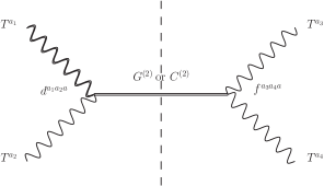
Figure 3: Factorization of the amplitude $\mathcal{A}(G^{(1)},g,g,g)$ gives different group factors on two sides. The doubled wavy line presents the first massive-level bosonic string state, whereas the single lines present massless bosonic string states. $G^{(2)}$ or $C^{(2)}$ are the second massive-level intermediate string states obtained from factorization.

In this section all the four-point amplitudes with one first massive-level string state are taken from Ref. [11]. In Ref. [11], the massive string state was placed at position 4, and the three massless ones took the positions 1, 2, and 3. For our convenience, in this work we prefer to place the massive string state at position 1, while the three massless string states were placed at 2, 3, and 4. The corresponding amplitudes can be easily obtained by performing permutations of the original amplitudes.

The helicity wave function of a massive higher spin particle is specified by a pair of lightlike vectors $p^{\mu},q^{\mu}$, which is a decomposition of the momentum of the particle $k^{\mu}=p^{\mu}+q^{\mu}$. The spin quantization axis is along the direction of $\vec{q}$ in the rest frame; here, it is most convenient to set $q^{\mu}=k_{2}^{\mu}$, so that the spin axis of the first massive-level string state (at position 1) is along the same direction as the spin axis of the massless string state at position 2, and we denote this direction to be $+\vec{z}$. Because of angular momentum conservation, the spin axis of the intermediate second massive-level string state (see Fig. 3) should also align to $+\vec{z}$, and the corresponding helicity amplitudes of these three states with only specific $j_{z}$ combinations can survive. The reference momenta of particle 1 are chosen to be

$$p^{\mu}=\left(\frac{\sqrt{s}}{2},0,0,-\frac{\sqrt{s}}{2}\right)\,,\quad q^{\mu}=k_{2}^{\mu}=\left(\frac{M_{s}^{2}}{2\sqrt{s}},0,0,\frac{M_{s}^{2}}{2\sqrt{s}}\right)\,.$$ (4.1)

The spinor products become

$$\langle p2\rangle[2p]=s/2\,,\quad\langle p3\rangle[3p]=2t\,,\quad\langle p4\rangle[4p]=2u\,,$$ (4.2)

where $s,t,u$ are Mandelstam variables. With this choice, we could extract the helicity amplitudes of the second massive-level strings decaying into a first massive-level string plus a massless one with their spin axes all along $+\vec{z}$ (the direction of the momentum of the massless string state), from the four-point amplitudes in Ref. [11]. In the next section, we will focus on the spin-3 and spin-2 universal string states from the second massive level, computing their scattering amplitudes and their partial decay widths, where we will also align the spins of the three interacting states in the direction of the momentum of the massless particle. Thus, we are expecting the helicity amplitudes we obtained from factorization in this section to match exactly with the string amplitudes from CFT computations in the next section.

We will discuss the factorization of the four-point amplitudes in the following order. We start from the amplitudes which involve the first massive-level spin-2 field $\alpha$ and obtain the decay widths of second massive-level string states decaying into $\alpha$ plus another massless string state. Then we discuss the decays which involve the final states $d,\Phi,\chi,a$ in order, which are obtained from the four-point amplitudes with $d,\Phi,\chi,a$ plus three other massless string states. The full results of decay widths for $n=2$ resonances are summarized in Table 4 at the end of this section.

4.2 $\alpha(J=2)$

The highest spin field from the first massive level is the spin-2 boson $\alpha$ with its vertex operator given in Eq. (5.4). We will need to use the amplitudes (all particles are incoming) [11]

$$\mathcal{A}[\alpha_{1},\epsilon_{2},\epsilon_{3},\epsilon_{4}] = 8\,g_{3}^{2}\big{(}\,V_{t}\,t^{a_{1}a_{2}a_{3}a_{4}}+V_{s}\,t^{a_{2}a_{3}a_{1}a_{4}}+V_{u}\,t^{a_{3}a_{1}a_{2}a_{4}}\,\big{)}\sqrt{2\alpha^{\prime}}\ \mathscr{A}[\alpha_{1},\epsilon_{2},\epsilon_{3},\epsilon_{4}],\quad$$ (4.3)

$$\mathcal{A}[\alpha_{1},u_{2},\bar{u}_{3},\epsilon_{4}] = 2\,g_{3}^{2}\ \big{[}V_{t}(T^{a_{4}}T^{a_{1}})^{\alpha_{2}}_{\alpha_{3}}+V_{s}(T^{a_{1}}T^{a_{4}})^{\alpha_{2}}_{\alpha_{3}}\big{]}\ \sqrt{2\alpha^{\prime}}\ \mathscr{A}[\alpha_{1},u_{2},\bar{u}_{3},\epsilon_{4}]\,,$$ (4.4)

where $\epsilon$ denotes the polarization vector of a gluon $g$, and

$$\mathscr{A}\left[\alpha(+2),+,+,-\right] =\frac{1}{2\sqrt{2}}\ \!\frac{\langle p4\rangle^{4}}{\langle 23\rangle\langle 34\rangle\langle 42\rangle}\,,$$

$$\mathscr{A}\left[\alpha(+1),+,+,-\right] =\frac{1}{\sqrt{2}}\ \,\frac{\langle p4\rangle^{3}\langle 4q\rangle}{\langle 23\rangle\langle 34\rangle\langle 42\rangle}\,,$$

$$\mathscr{A}\left[\alpha(\leavevmode\nobreak\ 0\leavevmode\nobreak\ ),+,+,-\right] =\frac{\sqrt{3}}{2}\ \,\frac{\langle p4\rangle^{2}\langle 4q\rangle^{2}}{\langle 23\rangle\langle 34\rangle\langle 42\rangle}\,,$$ (4.5)

$$\mathscr{A}\left[\alpha(-1),+,+,-\right] =\frac{1}{\sqrt{2}}\ \,\frac{\langle q4\rangle^{3}\langle 4p\rangle}{\langle 23\rangle\langle 34\rangle\langle 42\rangle}\,,$$

$$\mathscr{A}\left[\alpha(-2),+,+,-\right] =\frac{1}{2\sqrt{2}}\ \!\frac{\langle q4\rangle^{4}}{\langle 23\rangle\langle 34\rangle\langle 42\rangle}\,,$$

and

$$\mathscr{A}\left[\alpha(+2),{+}{\textstyle\frac{1}{2}},{-}{\textstyle\frac{1}{2}},+\right] =\frac{1}{\sqrt{2}}\ \frac{\langle p2\rangle\langle p3\rangle^{3}}{\langle 23\rangle\langle 34\rangle\langle 42\rangle}\,,$$

$$\mathscr{A}\left[\alpha(+1),{+}{\textstyle\frac{1}{2}},{-}{\textstyle\frac{1}{2}},+\right] =\frac{1}{2\sqrt{2}}\,\frac{\langle p3\rangle^{2}}{\langle 23\rangle\langle 34\rangle\langle 42\rangle}\big{(}\langle q2\rangle\langle p3\rangle+3\langle p2\rangle\langle q3\rangle\big{)}\,,$$

$$\mathscr{A}\left[\alpha(\leavevmode\nobreak\ 0\leavevmode\nobreak\ ),{+}{\textstyle\frac{1}{2}},{-}{\textstyle\frac{1}{2}},+\right] =\frac{\sqrt{3}}{2}\ \frac{\langle p3\rangle\langle q3\rangle}{\langle 23\rangle\langle 34\rangle\langle 42\rangle}\ \big{(}\langle q2\rangle\langle p3\rangle+\langle p2\rangle\langle q3\rangle\big{)}\,,$$ (4.6)

$$\mathscr{A}\left[\alpha(-1),{+}{\textstyle\frac{1}{2}},{-}{\textstyle\frac{1}{2}},+\right] =\frac{1}{2\sqrt{2}}\,\frac{\langle q3\rangle^{2}}{\langle 23\rangle\langle 34\rangle\langle 42\rangle}\big{(}3\langle q2\rangle\langle p3\rangle+\langle p2\rangle\langle q3\rangle\big{)}\,,$$

$$\mathscr{A}\left[\alpha(-2),{+}{\textstyle\frac{1}{2}},{-}{\textstyle\frac{1}{2}},+\right] =\frac{1}{\sqrt{2}}\ \frac{\langle q2\rangle\langle q3\rangle^{3}}{\langle 23\rangle\langle 34\rangle\langle 42\rangle}\,.$$

The other nonvanishing amplitudes can be obtained by taking the complex conjugate and permutation.

4.2.1 $G^{(2)}(J=3,2)\to\alpha+g$

We now factorize the four-point amplitudes $\mathcal{A}[\alpha,+,+,-]$ to get the matrix elements of $G^{(2)}(J=2,3)$ decaying into $\alpha+g^{+}$. Amplitudes $\mathcal{A}[\alpha,-,-,+]$, can be obtained via the complex conjugate, and they give the matrix elements of the decays $G^{(2)}(J=3,2)\to\alpha+g^{-}$. The factorization of $\mathcal{A}[\alpha(+2),+,+,-]$ gives

$$\mathcal{A}[\alpha(+2),+,+,-]=\frac{g_{3}^{2}M_{s}^{2}}{s-2M_{s}^{2}}\frac{16}{\sqrt{3}}d^{3}_{-3,-2}(\theta)\,f^{a_{1}a_{2}a}d^{a_{3}a_{4}a}\,,$$ (4.7)

where $\theta$ is the angle between $-\vec{z}$ and the spatial momentum of particle $3$. It is related to the Mandelstam variables $u,t$ by

$$u=-\frac{s}{2}(1+\cos\theta)\,,\leavevmode\nobreak\ \leavevmode\nobreak\ \leavevmode\nobreak\ t=-\frac{s}{2}(1-\cos\theta)\,.$$ (4.8)

From (4.7) we can read off the matrix elements as,

$$F^{a,J=3}_{+2+a_{1}a_{2}}=F^{a,J=3}_{-2-a_{1}a_{2}}=8g_{3}M_{s}d^{a_{1}a_{2}a}\,,$$ (4.9)

where we use $F^{a,J}_{\lambda_{1}\lambda_{2}a_{1}a_{2}}$ to denote the amplitude of a spin-$J$ particle with angular momentum $j_{z}=\lambda_{1}+\lambda_{2}$ (and gauge index $a$) decaying into particles 1 and 2 with momenta along the $\vec{z}$ axis. $\lambda_{1},\lambda_{2}$ are helicities of the two particles while $a_{1},a_{2}$ are gauge indices. Thus, the result of Eq. (4.9) presents the decay of a second massive-level spin-3 string state with $j_{z}=-3$ decaying into $\alpha_{1}(j_{z}=-2)$ and $\epsilon_{2}^{-}$, which is exactly what we get in Eq. (5.48) in the next section. In Eq. (5.48), all particles are incoming and the corresponding outgoing particles are one ${\alpha}(-2)$ and one ${\epsilon}^{-}$. We would like to remind the reader that the definition of $F^{a,J}_{\lambda_{1}\lambda_{2}a_{1}a_{2}}$ is in some sense different from what is used in the literature [22, 23, 7]. Previously the helicity ${\lambda}_{1}$ (of a massless particle) was usually defined with its spin axis along $\vec{k}_{1}$. In our convention the spin axis of every particle is along $+\vec{z}$. Particle $1$ is moving along $-\vec{z}$ and its spin axis is opposite to $\vec{k}_{1}$.

Similarly, we can do the factorization for amplitudes with other spin configurations:

$$\mathcal{A}[\alpha(+1),+,+,-]=\frac{g_{3}^{2}M_{s}^{2}}{s-2M_{s}^{2}}\left(\frac{16}{3}d^{3}_{-2,-2}(\theta)-\frac{16}{3}d^{2}_{-2,-2}(\theta)\right)f^{a_{1}a_{2}a}d^{a_{3}a_{4}a}\,,$$ (4.10)

$$F^{a,J=3}_{+1+a_{1}a_{2}}=F^{a,J=3}_{-1-a_{1}a_{2}}=\frac{8}{\sqrt{3}}g_{3}M_{s}d^{a_{1}a_{2}a}\,,\quad F^{a,J=2}_{+1+a_{1}a_{2}}=F^{a,J=2}_{-1-a_{1}a_{2}}=4\sqrt{\frac{2}{3}}g_{3}M_{s}d^{a_{1}a_{2}a}\,.$$ (4.11)

$$\mathcal{A}[\alpha(0),+,+,-]=\frac{g_{3}^{2}M_{s}^{2}}{s-2M_{s}^{2}}\left(8\sqrt{\frac{2}{15}}d^{3}_{-1,-2}(\theta)-\frac{8}{\sqrt{3}}d^{2}_{-1,-2}(\theta)\right)f^{a_{1}a_{2}a}d^{a_{3}a_{4}a}\,,$$ (4.12)

$$F^{a,J=3}_{0+a_{1}a_{2}}=F^{a,J=3}_{0-a_{1}a_{2}}=4\sqrt{\frac{2}{5}}g_{3}M_{s}d^{a_{1}a_{2}a}\,,\quad F^{a,J=2}_{0+a_{1}a_{2}}=F^{a,J=2}_{0-a_{1}a_{2}}=2\sqrt{2}g_{3}M_{s}d^{a_{1}a_{2}a}\,.$$ (4.13)

$$\mathcal{A}[\alpha(-1),+,+,-]=\frac{g_{3}^{2}M_{s}^{2}}{s-2M_{s}^{2}}\left(4\sqrt{\frac{2}{15}}d^{3}_{0,-2}(\theta)-4\sqrt{\frac{2}{3}}d^{2}_{0,-2}(\theta)\right)f^{a_{1}a_{2}a}d^{a_{3}a_{4}a}\,,$$ (4.14)

$$F^{a,J=3}_{-1+a_{1}a_{2}}=F^{a,J=3}_{+1-a_{1}a_{2}}=2\sqrt{\frac{2}{5}}g_{3}M_{s}d^{a_{1}a_{2}a}\,,\quad F^{a,J=2}_{-1+a_{1}a_{2}}=F^{a,J=2}_{+1-a_{1}a_{2}}=2g_{3}M_{s}d^{a_{1}a_{2}a}\,.$$ (4.15)

$$\mathcal{A}[\alpha(-2),+,+,-]=\frac{g_{3}^{2}M_{s}^{2}}{s-2M_{s}^{2}}\left(\frac{4}{3\sqrt{5}}d^{3}_{+1,-2}(\theta)-\frac{4\sqrt{2}}{3}d^{2}_{+1,-2}(\theta)\right)f^{a_{1}a_{2}a}d^{a_{3}a_{4}a}\,,$$ (4.16)

$$F^{a,J=3}_{-2+a_{1}a_{2}}=F^{a,J=3}_{+2-a_{1}a_{2}}=\frac{2}{\sqrt{15}}g_{3}M_{s}d^{a_{1}a_{2}a}\,,\quad F^{a,J=2}_{-2+a_{1}a_{2}}=F^{a,J=2}_{+2-a_{1}a_{2}}=\frac{2}{\sqrt{3}}g_{3}M_{s}d^{a_{1}a_{2}a}\,.$$ (4.17)

The decay width can be computed using (an extra factor of $1/2$ is needed if outgoing particles are a pair of gluons)

$$\Gamma^{aJ}_{\lambda_{1}\lambda_{2},a_{1}a_{2}}=\frac{1}{32(2J+1)\sqrt{2}\pi M_{s}}|F^{aJ}_{\lambda_{1}\lambda_{2},a_{1}a_{2}}|^{2}\,.$$ (4.18)

We need to take into account both the channels into $\alpha+g^{+}$ and into $\alpha+g^{-}$ and the results are

$$\Gamma^{J=3}_{G^{(2)}\rightarrow\alpha g}=\frac{117g_{3}^{2}M_{s}}{2240\sqrt{2}\pi}N\,,\qquad\Gamma^{J=2}_{G^{(2)}\rightarrow\alpha g}=\frac{3g_{3}^{2}M_{s}}{160\sqrt{2}\pi}N\,.$$ (4.19)

4.2.2 $G^{(2)}(J=1)\to\alpha+g$

The spin-1 resonances arise from factorization of the amplitude $\mathcal{A}[\alpha,-,+,+]$,

$$\mathcal{A}[\alpha(+2),-,+,+]=\frac{4g_{3}^{2}M_{s}^{2}}{s-2M_{s}^{2}}d^{1}_{-1,0}(\theta)f^{a_{1}a_{2}a}d^{a_{3}a_{4}a}\,,$$ (4.20)

and we obtain

$$F^{a,J=1}_{+2-a_{1}a_{2}}=F^{a,J=1}_{-2+a_{1}a_{2}}=2g_{3}M_{s}d^{a_{1}a_{2}a}\,,$$ (4.21)

which corresponds to the complex vectors found in Ref. [12]. Unlike $G^{(2)}(J=3,2)$, $G^{(2)}(J=1)$ is not parity invariant, the matrix elements in (4.21) are for two different particles and should not be added together. Thus the corresponding partial decay width reads

$$\Gamma^{J=1}_{G^{(2)}\rightarrow\alpha g}=\frac{g_{3}^{2}M_{s}}{384\sqrt{2}\pi}N\,.$$ (4.22)

4.2.3 $Q^{(2)}(J=5/2,3/2)\to\alpha+q$

We could obtain the second massive-level spin-$\frac{5}{2}$ and spin-$\frac{3}{2}$ resonances from factorizing amplitude $\mathcal{A}[\alpha,+\tfrac{1}{2},-\tfrac{1}{2},+]$:

$$\mathcal{A}\left[\alpha(+2),+\tfrac{1}{2},-\tfrac{1}{2},+\right]=\frac{g_{3}^{2}M_{s}^{2}}{s-2M_{s}^{2}}\frac{4}{\sqrt{5}}d^{5/2}_{-5/2,+3/2}(\theta)T^{a_{1}}_{\alpha_{2}\alpha}T^{a_{4}}_{\alpha\alpha_{3}}\,,$$ (4.23)

$$F^{{\alpha},J=5/2}_{+2+\frac{1}{2}a_{1}{\alpha}_{2}}=F^{{\alpha},J=5/2}_{-2-\frac{1}{2}a_{1}{\alpha}_{2}}=\sqrt{2}g_{3}M_{s}T^{a_{1}}_{\alpha_{2}\alpha}\,.$$ (4.24)

$$\mathcal{A}\left[\alpha(+1),+\tfrac{1}{2},-\tfrac{1}{2},+\right]=\frac{g_{3}^{2}M_{s}^{2}}{s-2M_{s}^{2}}\left(\frac{3\sqrt{2}}{5}d^{5/2}_{-3/2,+3/2}(\theta)-\frac{3\sqrt{2}}{5}d^{3/2}_{-3/2,+3/2}(\theta)\right)T^{a_{1}}_{\alpha_{2}\alpha}T^{a_{4}}_{\alpha\alpha_{3}}\,,$$ (4.25)

$$F^{{\alpha},J=5/2}_{+1+\frac{1}{2}a_{1}{\alpha}_{2}}=F^{{\alpha},J=5/2}_{-1-\frac{1}{2}a_{1}{\alpha}_{2}}=\frac{3}{2\sqrt{5}}g_{3}M_{s}T^{a_{1}}_{\alpha_{2}\alpha}\,,\quad F^{{\alpha},J=3/2}_{+1+\frac{1}{2}a_{1}{\alpha}_{2}}=F^{{\alpha},J=3/2}_{-1-\frac{1}{2}a_{1}{\alpha}_{2}}=\sqrt{\frac{3}{10}}g_{3}M_{s}T^{a_{1}}_{\alpha_{2}\alpha}\,.$$ (4.26)

$$\mathcal{A}\left[\alpha(0),+\tfrac{1}{2},-\tfrac{1}{2},+\right]=\frac{g_{3}^{2}M_{s}^{2}}{s-2M_{s}^{2}}\left(-\frac{\sqrt{3}}{5}d^{5/2}_{-1/2,+3/2}(\theta)-\frac{2\sqrt{2}}{5}d^{3/2}_{-1/2,+3/2}(\theta)\right)T^{a_{1}}_{\alpha_{2}\alpha}T^{a_{4}}_{\alpha\alpha_{3}}\,,$$ (4.27)

$$F^{{\alpha},J=5/2}_{0+\frac{1}{2}a_{1}{\alpha}_{2}}=F^{{\alpha},J=5/2}_{0-\frac{1}{2}a_{1}{\alpha}_{2}}=\frac{1}{2}\sqrt{\frac{3}{10}}g_{3}M_{s}T^{a_{1}}_{\alpha_{2}\alpha}\,,\quad F^{{\alpha},J=3/2}_{0+\frac{1}{2}a_{1}{\alpha}_{2}}=F^{{\alpha},J=3/2}_{0-\frac{1}{2}a_{1}{\alpha}_{2}}=\sqrt{\frac{2}{15}}g_{3}M_{s}T^{a_{1}}_{\alpha_{2}\alpha}\,.$$ (4.28)

$$\mathcal{A}\left[\alpha(-1),+\tfrac{1}{2},-\tfrac{1}{2},+\right]=\frac{g_{3}^{2}M_{s}^{2}}{s-2M_{s}^{2}}\left(\frac{1}{10}d^{5/2}_{+1/2,+3/2}(\theta)-\frac{1}{5}\sqrt{\frac{3}{2}}d^{3/2}_{+1/2,+3/2}(\theta)\right)T^{a_{1}}_{\alpha_{2}\alpha}T^{a_{4}}_{\alpha\alpha_{3}}\,,$$ (4.29)

$$F^{{\alpha},J=5/2}_{-1+\frac{1}{2}a_{1}{\alpha}_{2}}=F^{{\alpha},J=5/2}_{+1-\frac{1}{2}a_{1}{\alpha}_{2}}=\frac{1}{4\sqrt{10}}g_{3}M_{s}T^{a_{1}}_{\alpha_{2}\alpha}\,,\quad F^{{\alpha},J=3/2}_{-1+\frac{1}{2}a_{1}{\alpha}_{2}}=F^{{\alpha},J=3/2}_{+1-\frac{1}{2}a_{1}{\alpha}_{2}}=\frac{1}{2\sqrt{10}}g_{3}M_{s}T^{a_{1}}_{\alpha_{2}\alpha}\,.$$ (4.30)

Left-handed and right-handed fermions are stretching between different branes. As a result, left-handed excited quarks cannot decay into right-handed quarks plus gluons. For example, we have $F^{{\alpha},J=5/2}_{+2+\frac{1}{2}a_{1}\alpha_{2}}=F^{{\alpha},J=5/2}_{-2-\frac{1}{2}a_{1}\alpha_{2}}$ but they are decay amplitudes for left- and right-handed excited quarks and should not be combined. The corresponding decay widths are

$$\Gamma^{J=5/2}_{Q^{(2)}\rightarrow\alpha q}=\frac{27g_{3}^{2}M_{s}}{4096\sqrt{2}\pi}N\,,\qquad\Gamma^{J=3/2}_{Q^{(2)}\rightarrow\alpha q}=\frac{11g_{3}^{2}M_{s}}{6144\sqrt{2}\pi}N\,.$$ (4.31)

4.2.4 $Q^{(2)}(J=3/2,1/2)\to\alpha+q$

The second massive-level spin-$\frac{3}{2}$ and spin-$\frac{1}{2}$ resonances can be obtained from amplitude $\mathcal{A}[\alpha,-\frac{1}{2},+,+\frac{1}{2}]$:

$$\mathcal{A}\left[\alpha(+2),-\tfrac{1}{2},+,+\tfrac{1}{2}\right]=\frac{g_{3}^{2}M_{s}^{2}}{s-2M_{s}^{2}}\frac{2}{\sqrt{3}}d^{3/2}_{-3/2,-1/2}(\theta)T^{a_{1}}_{\alpha_{2}\alpha}T^{a_{3}}_{\alpha\alpha_{4}}\,,$$ (4.32)

$$F^{{\alpha},J=3/2}_{+2-\frac{1}{2}a_{1}{\alpha}_{2}}=F^{{\alpha},J=3/2}_{-2+\frac{1}{2}a_{1}{\alpha}_{2}}=\frac{1}{\sqrt{2}}g_{3}M_{s}T^{a_{1}}_{\alpha_{2}\alpha}\,.$$ (4.33)

$$\mathcal{A}\left[\alpha(+1),-\tfrac{1}{2},+,+\tfrac{1}{2}\right]=\frac{g_{3}^{2}M_{s}^{2}}{s-2M_{s}^{2}}\left(\frac{1}{3\sqrt{2}}d^{3/2}_{-1/2,-1/2}(\theta)-\frac{1}{3\sqrt{2}}d^{1/2}_{-1/2,-1/2}(\theta)\right)T^{a_{1}}_{\alpha_{2}\alpha}T^{a_{3}}_{\alpha\alpha_{4}}\,,$$ (4.34)

$$F^{{\alpha},J=3/2}_{+1-\frac{1}{2}a_{1}{\alpha}_{2}}=F^{{\alpha},J=3/2}_{-1+\frac{1}{2}a_{1}{\alpha}_{2}}=\frac{1}{4\sqrt{3}}g_{3}M_{s}T^{a_{1}}_{\alpha_{2}\alpha}\,,\quad F^{{\alpha},J=1/2}_{+1-\frac{1}{2}a_{1}{\alpha}_{2}}=F^{{\alpha},J=1/2}_{-1+\frac{1}{2}a_{1}{\alpha}_{2}}=\frac{1}{2\sqrt{6}}g_{3}M_{s}T^{a_{1}}_{\alpha_{2}\alpha}\,.$$ (4.35)

The spin-$\frac{3}{2}$ fermion $\tilde{Q}^{(2)}$ here is different from the spin-$\frac{3}{2}$ fermion $Q^{(2)}$ we obtained from the amplitude $\mathcal{A}[\alpha,+\tfrac{1}{2},-\tfrac{1}{2},+]$, as this one can decay into $(+,+\frac{1}{2})$ (instead of $(-,+\frac{1}{2})$). Since the amplitude $\mathcal{A}[+,+,+\frac{1}{2},-\frac{1}{2}]=0$, these two states do not mix, and we obtain

$$\Gamma^{J=3/2}_{\tilde{Q}^{(2)}\rightarrow\alpha q}=\frac{25g_{3}^{2}M_{s}}{12288\sqrt{2}\pi}N\,,\qquad\Gamma^{J=1/2}_{Q^{(2)}\rightarrow\alpha q}=\frac{g_{3}^{2}M_{s}}{3072\sqrt{2}\pi}N\,.$$ (4.36)

4.3 $d(J=1)$

The spin-1 field $d$ is different from the universal bosonic fields $\alpha,\Phi$ in that it is tied to spacetime SUSY. Although its vertex operator contains the world sheet current $\mathcal{J}$, the vector $d$ does give rise to universal amplitudes into a quark-antiquark pair [11]. The existence of this vector resonance is a universal property of all $\mathcal{N}=1$ SUSY compactifications. We will need the amplitude $\mathcal{A}[d_{1},u_{2},\bar{u}_{3},\epsilon_{4}]$, which reads

$$\mathcal{A}[d_{1},u_{2},\bar{u}_{3},\epsilon_{4}]=\sqrt{3}\,g_{3}^{2}\ \big{[}V_{t}(T^{a_{4}}T^{a_{1}})^{\alpha_{2}}_{\alpha_{3}}+V_{s}(T^{a_{1}}T^{a_{4}})^{\alpha_{2}}_{\alpha_{3}}\big{]}\ \mathscr{A}\left[d_{1},u_{2},\bar{u}_{3},\epsilon_{4}\right]\,,$$ (4.37)

where

$$\mathscr{A}\left[d(+1),{+}{\textstyle\frac{1}{2}},{-}{\textstyle\frac{1}{2}},+\right] =\frac{\langle p3\rangle^{2}}{\langle 24\rangle\langle 34\rangle}\,,$$

$$\mathscr{A}\left[d(\leavevmode\nobreak\ 0\leavevmode\nobreak\ ),{+}{\textstyle\frac{1}{2}},{-}{\textstyle\frac{1}{2}},+\right] =\sqrt{2}\,\frac{\langle p3\rangle\langle q3\rangle}{\langle 24\rangle\langle 34\rangle}\,,$$ (4.38)

$$\mathscr{A}\left[d(-1),{+}{\textstyle\frac{1}{2}},{-}{\textstyle\frac{1}{2}},+\right] =-\frac{\langle q3\rangle^{2}}{\langle 24\rangle\langle 34\rangle}\,.$$

These amplitudes will give rise to two channels of the second massive-level string resonances.

4.3.1 $Q^{(2)}(J=5/2,3/2)\to d+q$

We could obtain the second massive-level spin-$\frac{5}{2}$ and spin-$\frac{3}{2}$ resonances from factorizing amplitude $\mathcal{A}[d,+\frac{1}{2},-\frac{1}{2},+]$:

$$\mathcal{A}[d(+1),+\tfrac{1}{2},-\tfrac{1}{2},+]=\frac{g_{3}^{2}M_{s}^{2}}{s-2M_{s}^{2}}\left(\frac{\sqrt{6}}{5}d^{5/2}_{-3/2,+3/2}(\theta)+\frac{\sqrt{6}}{5}d^{3/2}_{-3/2,+3/2}(\theta)\right)T^{a_{1}}_{\alpha_{2}\alpha}T^{a_{4}}_{\alpha\alpha_{3}}\,,$$ (4.39)

$$F^{{\alpha},J=5/2}_{+1+\frac{1}{2}a_{1}{\alpha}_{2}}=F^{{\alpha},J=5/2}_{-1-\frac{1}{2}a_{1}{\alpha}_{2}}=\frac{1}{2}\sqrt{\frac{3}{5}}g_{3}M_{s}T^{a_{1}}_{\alpha_{2}\alpha}\,,\quad F^{{\alpha},J=3/2}_{+1+\frac{1}{2}a_{1}{\alpha}_{2}}=F^{{\alpha},J=3/2}_{-1-\frac{1}{2}a_{1}{\alpha}_{2}}=\frac{1}{\sqrt{10}}g_{3}M_{s}T^{a_{1}}_{\alpha_{2}\alpha}\,.$$ (4.40)

$$\mathcal{A}[d(0),+\tfrac{1}{2},-\tfrac{1}{2},+]=\frac{g_{3}^{2}M_{s}^{2}}{s-2M_{s}^{2}}\left(\frac{\sqrt{3}}{5}d^{5/2}_{-1/2,+3/2}(\theta)+\frac{2\sqrt{2}}{5}d^{3/2}_{-1/2,+3/2}(\theta)\right)T^{a_{1}}_{\alpha_{2}\alpha}T^{a_{4}}_{\alpha\alpha_{3}}\,,$$ (4.41)

$$F^{{\alpha},J=5/2}_{0+\frac{1}{2}a_{1}{\alpha}_{2}}=F^{{\alpha},J=5/2}_{0-\frac{1}{2}a_{1}{\alpha}_{2}}=\frac{1}{2}\sqrt{\frac{3}{10}}g_{3}M_{s}T^{a_{1}}_{\alpha_{2}\alpha}\,,\quad F^{{\alpha},J=3/2}_{0+\frac{1}{2}a_{1}{\alpha}_{2}}=F^{{\alpha},J=3/2}_{0-\frac{1}{2}a_{1}{\alpha}_{2}}=\sqrt{\frac{2}{15}}g_{3}M_{s}T^{a_{1}}_{\alpha_{2}\alpha}\,.$$ (4.42)

$$\mathcal{A}[d(-1),+\tfrac{1}{2},-\tfrac{1}{2},+]=\frac{g_{3}^{2}M_{s}^{2}}{s-2M_{s}^{2}}\left(\frac{\sqrt{3}}{10}d^{5/2}_{+1/2,+3/2}(\theta)+\frac{3}{5\sqrt{2}}d^{3/2}_{+1/2,+3/2}(\theta)\right)T^{a_{1}}_{\alpha_{2}\alpha}T^{a_{4}}_{\alpha\alpha_{3}}\,,$$ (4.43)

$$F^{{\alpha},J=5/2}_{-1+\frac{1}{2}a_{1}{\alpha}_{2}}=F^{{\alpha},J=5/2}_{+1-\frac{1}{2}a_{1}{\alpha}_{2}}=\frac{1}{4}\sqrt{\frac{3}{10}}g_{3}M_{s}T^{a_{1}}_{\alpha_{2}\alpha}\,,\quad F^{{\alpha},J=3/2}_{-1+\frac{1}{2}a_{1}{\alpha}_{2}}=F^{{\alpha},J=3/2}_{+1-\frac{1}{2}a_{1}{\alpha}_{2}}=\frac{1}{2}\sqrt{\frac{3}{10}}g_{3}M_{s}T^{a_{1}}_{\alpha_{2}\alpha}\,.$$ (4.44)

The corresponding partial decay widths read

$$\Gamma^{J=5/2}_{Q^{(2)}\rightarrow dq}=\frac{13g_{3}^{2}M_{s}}{20480\sqrt{2}\pi}N\,,\qquad\Gamma^{J=3/2}_{Q^{(2)}\rightarrow dq}=\frac{37g_{3}^{2}M_{s}}{30720\sqrt{2}\pi}N\,.$$ (4.45)

4.3.2 $Q^{(2)}(J=3/2,1/2)\to d+q$

The second massive-level spin-$\frac{3}{2}$ and spin-$\frac{1}{2}$ resonances arise from amplitude $\mathcal{A}[d,-\frac{1}{2},+,+\frac{1}{2}]$:

$$\mathcal{A}[d(+1),-\frac{1}{2},+,+\frac{1}{2}]=\frac{g_{3}^{2}M_{s}^{2}}{s-2M_{s}^{2}}\left(\frac{1}{\sqrt{6}}d^{3/2}_{-1/2,-1/2}(\theta)-\frac{1}{\sqrt{6}}d^{1/2}_{-1/2,-1/2}(\theta)\right)T^{a_{1}}_{\alpha_{2}\alpha}T^{a_{3}}_{\alpha\alpha_{4}}\,,$$ (4.46)

$$F^{{\alpha},J=3/2}_{+1-\frac{1}{2}a_{1}{\alpha}_{2}}=F^{{\alpha},J=3/2}_{-1+\frac{1}{2}a_{1}{\alpha}_{2}}=\frac{1}{4}g_{3}M_{s}T^{a_{1}}_{\alpha_{2}\alpha}\,,\quad F^{{\alpha},J=1/2}_{+1-\frac{1}{2}a_{1}{\alpha}_{2}}=F^{{\alpha},J=1/2}_{-1+\frac{1}{2}a_{1}{\alpha}_{2}}=\frac{1}{2\sqrt{2}}g_{3}M_{s}T^{a_{1}}_{\alpha_{2}\alpha}\,,$$ (4.47)

and the corresponding partial decay widths read

$$\Gamma^{J=3/2}_{\tilde{Q}^{(2)}\rightarrow dq}=\frac{g_{3}^{2}M_{s}}{4096\sqrt{2}\pi}N\,,\qquad\Gamma^{J=1/2}_{Q^{(2)}\rightarrow dq}=\frac{g_{3}^{2}M_{s}}{1024\sqrt{2}\pi}N\,.$$ (4.48)

Similar to previous case, we identify the spin-$\frac{3}{2}$ fermion in this channel as $\tilde{Q}^{(2)}(J=3/2)$.

4.4 $\Phi_{\pm}(J=0)$

$\Phi$ is a complex scalar field, which couples to only (anti)self-dual gauge field configurations, i.e., to gluons in $(++)$ or $(--)$ helicity configurations. The vertex operator of $\Phi$ is given in Eq. (5.5). We will use the following amplitudes:

$$\mathcal{A}[\Phi_{+},+,+,-] =4\,g_{3}^{2}\big{(}\,V_{t}\,t^{a_{1}a_{2}a_{3}a_{4}}+V_{s}\,t^{a_{2}a_{3}a_{1}a_{4}}+V_{u}\,t^{a_{3}a_{1}a_{2}a_{4}}\,\big{)}\sqrt{\alpha^{\prime}}\frac{[23]^{4}}{[23][34][42]},\quad$$ (4.49)

$$\mathcal{A}[\Phi_{+},+,+,+] =4\,g_{3}^{2}\big{(}\,V_{t}\,t^{a_{1}a_{2}a_{3}a_{4}}+V_{s}\,t^{a_{2}a_{3}a_{1}a_{4}}+V_{u}\,t^{a_{3}a_{1}a_{2}a_{4}}\,\big{)}\frac{(\alpha^{\prime})^{-3/2}}{\langle 23\rangle\langle 34\rangle\langle 42\rangle},$$ (4.50)

$$\mathcal{A}\left[\Phi_{+},+\tfrac{1}{2},-\tfrac{1}{2},+\right] =2g_{3}^{2}\big{[}V_{t}(T^{a_{4}}T^{a_{1}})^{\alpha_{2}}_{\alpha_{3}}+V_{s}(T^{a_{1}}T^{a_{4}})^{\alpha_{2}}_{\alpha_{3}}\big{]}\,\sqrt{\alpha^{\prime}}\,\frac{[24]^{2}}{[23]}\,.$$ (4.51)

4.4.1 $G^{(2)}(J=3,2)\to\Phi_{+}+g^{+}$

The second massive-level spin-3 and spin-2 excitations arise from factorization of $\mathcal{A}[\Phi_{+},+,+,-]$:

$$\mathcal{A}[\Phi_{+},+,+,-]=\frac{g_{3}^{2}M_{s}^{2}}{s-2M_{s}^{2}}\left(\frac{4}{3\sqrt{5}}d^{3}_{-1,-2}(\theta)+\frac{4\sqrt{2}}{3}d^{2}_{-1,-2}(\theta)\right)f^{a_{1}a_{2}a}d^{a_{3}a_{4}a}\,,$$ (4.52)

$$F^{a,J=3}_{\Phi_{+}+a_{1}a_{2}}=F^{a,J=3}_{\Phi_{-}-a_{1}a_{2}}=\frac{2}{\sqrt{15}}g_{3}M_{s}d^{a_{1}a_{2}a}\,,\quad F^{a,J=2}_{\Phi_{+}+a_{1}a_{2}}=F^{a,J=2}_{\Phi_{-}-a_{1}a_{2}}=\frac{2}{\sqrt{3}}g_{3}M_{s}d^{a_{1}a_{2}a}\,.$$ (4.53)

$G^{(2)}(J=3,2)$ can decay both into $\Phi_{+}+g^{+}$ and $\Phi_{-}+g^{-}$ (from $\mathcal{A}[\Phi_{-},-,-,+]$). However, $\Phi_{+}+g^{-}$ is not possible since $\mathcal{A}[\Phi_{+},+,-,-]=0$, and neither is $\Phi_{-}+g^{+}$ as $\mathcal{A}[\Phi_{-},-,+,+]=0$. These will also be confirmed in the next section. The corresponding decay widths read

$$\Gamma^{J=3}_{G^{(2)}\rightarrow\Phi g}=\frac{g_{3}^{2}M_{s}}{6720\sqrt{2}\pi}N\,,\qquad\Gamma^{J=2}_{G^{(2)}\rightarrow\Phi g}=\frac{g_{3}^{2}M_{s}}{960\sqrt{2}\pi}N\,.$$ (4.54)

4.4.2 $G^{(2)}(J=1)\to\Phi_{+}+g$

$G^{(2)}(J=1)$ can arise from the following two channels.

$G^{(2)}(J=1)\to\Phi_{+}+g^{+}$:

$$\mathcal{A}[\Phi_{+},+,+,+]=\frac{4g_{3}^{2}M_{s}^{2}}{s-2M_{s}^{2}}d^{1}_{-1,0}(\theta)f^{a_{1}a_{2}a}d^{a_{3}a_{4}a}\,,$$ (4.55)

$$F^{a,J=1}_{\Phi_{+}+a_{1}a_{2}}=F^{a,J=1}_{\Phi_{-}-a_{1}a_{2}}=2g_{3}M_{s}d^{a_{1}a_{2}a}\,.$$ (4.56)

$G^{(2)}(J=1)\to\Phi_{+}+g^{-}$:

$$\mathcal{A}[\Phi_{+},-,+,+]=\frac{16g_{3}^{2}M_{s}^{2}}{s-2M_{s}^{2}}d^{1}_{+1,0}(\theta)f^{a_{1}a_{2}a}d^{a_{3}a_{4}a}\,,$$ (4.57)

$$F^{a,J=1}_{\Phi_{+}-a_{1}a_{2}}=F^{a,J=1}_{\Phi_{-}+a_{1}a_{2}}=8g_{3}M_{s}d^{a_{1}a_{2}a}\,.$$ (4.58)

The $G^{(2)}(J=1)$ that goes into $\Phi_{+}+g^{+}$ is not parity invariant. Instead, its partner decays into $\Phi_{-}+g^{-}$. On the other hand, both channels of $\Phi_{+}+g^{+}$ and $\Phi_{+}+g^{-}$ are possible and we need to add them up.

$$\Gamma^{J=1}_{G^{(2)}\rightarrow\Phi g}=\frac{17g_{3}^{2}M_{s}}{384\sqrt{2}\pi}N\,.$$ (4.59)

4.4.3 $Q^{(2)}(J=5/2,3/2)\to\Phi_{+}+q$

The second massive-level spin-$\frac{5}{2}$ and spin-$\frac{3}{2}$ resonances arise from

$$\mathcal{A}\left[\Phi_{+},+\tfrac{1}{2},-\tfrac{1}{2},+\right]=\frac{g_{3}^{2}M_{s}^{2}}{s-2M_{s}^{2}}\left(\frac{\sqrt{2}}{5}d^{5/2}_{-1/2,+3/2}(\theta)-\frac{2\sqrt{3}}{5}d^{3/2}_{-1/2,+3/2}(\theta)\right)T^{a_{1}}_{\alpha_{2}\alpha}T^{a_{4}}_{\alpha\alpha_{3}}\,,$$ (4.60)

$$F^{{\alpha},J=5/2}_{\Phi_{+}+\frac{1}{2}a_{1}{\alpha}_{2}}=F^{{\alpha},J=5/2}_{\Phi_{-}-\frac{1}{2}a_{1}{\alpha}_{2}}=\frac{1}{2\sqrt{5}}g_{3}M_{s}T^{a_{1}}_{\alpha_{2}\alpha}\,,\quad F^{{\alpha},J=3/2}_{\Phi_{+}+\frac{1}{2}a_{1}{\alpha}_{2}}=F^{{\alpha},J=3/2}_{\Phi_{-}-\frac{1}{2}a_{1}{\alpha}_{2}}=\frac{1}{\sqrt{5}}g_{3}M_{s}T^{a_{1}}_{\alpha_{2}\alpha}\,.$$ (4.61)

The corresponding partial decay widths read

$$\Gamma^{J=5/2}_{Q^{(2)}\rightarrow\Phi q}=\frac{g_{3}^{2}M_{s}}{7680\sqrt{2}\pi}N\,,\qquad\Gamma^{J=3/2}_{Q^{(2)}\rightarrow\Phi q}=\frac{g_{3}^{2}M_{s}}{1280\sqrt{2}\pi}N\,.$$ (4.62)

4.4.4 $Q^{(2)}(J=3/2,1/2)\to\Phi_{+}+q$

The second massive-level spin-$\frac{3}{2}$ and spin-$\frac{1}{2}$ resonances arise from

$$\mathcal{A}\left[\Phi_{+},-\tfrac{1}{2},+,+\tfrac{1}{2}\right]=\frac{g_{3}^{2}M_{s}^{2}}{s-2M_{s}^{2}}\left(\frac{4}{3}d^{3/2}_{+1/2,-1/2}(\theta)+\frac{4}{3}d^{1/2}_{+1/2,-1/2}(\theta)\right)T^{a_{1}}_{\alpha_{2}\alpha}T^{a_{3}}_{\alpha\alpha_{4}}\,,$$ (4.63)

$$F^{{\alpha},J=3/2}_{\Phi_{+}+\frac{1}{2}a_{1}{\alpha}_{2}}=F^{{\alpha},J=3/2}_{\Phi_{-}-\frac{1}{2}a_{1}{\alpha}_{2}}=\sqrt{\frac{2}{3}}g_{3}M_{s}T^{a_{1}}_{\alpha_{2}\alpha}\,,\quad F^{{\alpha},J=1/2}_{\Phi_{+}+\frac{1}{2}a_{1}{\alpha}_{2}}=F^{{\alpha},J=1/2}_{\Phi_{-}-\frac{1}{2}a_{1}{\alpha}_{2}}=\frac{2}{\sqrt{3}}g_{3}M_{s}T^{a_{1}}_{\alpha_{2}\alpha}\,.$$ (4.64)

The corresponding partial decay widths read

$$\Gamma^{J=3/2}_{\tilde{Q}^{(2)}\rightarrow\Phi q}=\frac{g_{3}^{2}M_{s}}{384\sqrt{2}\pi}N,\leavevmode\nobreak\ \leavevmode\nobreak\ \leavevmode\nobreak\ \leavevmode\nobreak\ \Gamma^{J=1/2}_{Q^{(2)}\rightarrow\Phi q}=\frac{g_{3}^{2}M_{s}}{96\sqrt{2}\pi}N\ .$$ (4.65)

Similar to previous cases, we identify the spin-$\frac{3}{2}$ fermion to be $\tilde{Q}^{(2)}(J=3/2)$.

4.5 $\chi(J=3/2)$

The vertex operator of the spin-$\frac{3}{2}$ fermion $\chi$ is given in Eq. (5.8). We will need to use the following amplitudes:

$$\mathcal{A}[\chi_{1},\epsilon_{2},\epsilon_{3},u_{4}]\leavevmode\nobreak\ =\leavevmode\nobreak\ 2\,g_{3}^{2}\,[\,V_{t}\,(T^{a_{2}}T^{a_{3}})^{\alpha_{4}}_{\alpha_{1}}\ -\ V_{s}\,(T^{a_{3}}T^{a_{2}})_{\alpha_{1}}^{\alpha_{4}}\,]\,\mathscr{A}[\chi_{1},\epsilon_{2},\epsilon_{3},u_{4}]\ ,$$ (4.66)

where

$$\mathscr{A}\left[\chi(-\tfrac{3}{2}),-,-,{+}{\textstyle\frac{1}{2}}\right] =\leavevmode\nobreak\ \frac{[4q]^{3}}{[23][34][42]}\,,$$

$$\mathscr{A}\left[\chi(-\tfrac{1}{2}),-,-,{+}{\textstyle\frac{1}{2}}\right] =\sqrt{3}\frac{[4q]^{2}[p4]}{[23][34][42]}\,,$$

$$\mathscr{A}\left[\chi(-\tfrac{1}{2}),-,-,{+}{\textstyle\frac{1}{2}}\right] =\sqrt{3}\frac{[4p]^{2}[q4]}{[23][34][42]}\,,$$ (4.67)

$$\mathscr{A}\left[\chi(-\tfrac{3}{2}),-,-,{+}{\textstyle\frac{1}{2}}\right] =\leavevmode\nobreak\ \frac{[4p]^{3}}{[23][34][42]}\,,$$

and

$$\mathscr{A}\left[\chi(-\tfrac{3}{2}),+,-,{+}{\textstyle\frac{1}{2}}\right] =\leavevmode\nobreak\ \leavevmode\nobreak\ \sqrt{\alpha^{\prime}}\frac{\langle p3\rangle^{3}}{\langle 23\rangle\langle 24\rangle}\,,$$

$$\mathscr{A}\left[\chi(-\tfrac{1}{2}),+,-,{+}{\textstyle\frac{1}{2}}\right] =\leavevmode\nobreak\ \sqrt{3\alpha^{\prime}}\,\frac{\langle p3\rangle^{2}\langle q3\rangle}{\langle 23\rangle\langle 24\rangle}\,,$$

$$\mathscr{A}\left[\chi(-\tfrac{1}{2}),+,-,{+}{\textstyle\frac{1}{2}}\right] =-\sqrt{3\alpha^{\prime}}\frac{\langle q3\rangle^{2}\langle p3\rangle}{\langle 23\rangle\langle 24\rangle}\,,$$ (4.68)

$$\mathscr{A}\left[\chi(-\tfrac{3}{2}),+,-,{+}{\textstyle\frac{1}{2}}\right] =\leavevmode\nobreak\ {-}\sqrt{\alpha^{\prime}}\frac{\langle q3\rangle^{3}}{\langle 23\rangle\langle 24\rangle}\,.$$

4.5.1 $G^{(2)}(J=3,2)\to\chi+\bar{q}$

The second massive level spin-3 and spin-2 excitations arise from factorization of $\mathcal{A}[\chi,+\frac{1}{2},-,+]$:

$$\mathcal{A}\left[\chi(+\tfrac{3}{2}),+\tfrac{1}{2},-,+\right]=\frac{g_{3}^{2}M_{s}^{2}}{s-2M_{s}^{2}}\left(\frac{2}{3}d^{3}_{-2,+2}(\theta)+\frac{2}{3}d^{2}_{-2,+2}(\theta)\right)T^{a}_{{\alpha}_{1}{\alpha}_{2}}f^{a_{3}a_{4}a}\,,$$ (4.69)

$$F^{a,J=3}_{+\frac{3}{2}+\frac{1}{2}{\alpha}_{1}{\alpha}_{2}}=F^{a,J=3}_{-\frac{3}{2}-\frac{1}{2}{\alpha}_{1}{\alpha}_{2}}=\frac{1}{\sqrt{3}}g_{3}M_{s}T^{a}_{{\alpha}_{1}{\alpha}_{2}}\,,\quad F^{a,J=2}_{+\frac{3}{2}+\frac{1}{2}{\alpha}_{1}{\alpha}_{2}}=F^{a,J=2}_{-\frac{3}{2}-\frac{1}{2}{\alpha}_{1}{\alpha}_{2}}=\frac{1}{\sqrt{6}}g_{3}M_{s}T^{a}_{{\alpha}_{1}{\alpha}_{2}}\,.$$ (4.70)

$$\mathcal{A}\left[\chi(+\tfrac{1}{2}),+\tfrac{1}{2},-,+\right]=\frac{g_{3}^{2}M_{s}^{2}}{s-2M_{s}^{2}}\left(\frac{2}{\sqrt{15}}d^{3}_{-1,+2}(\theta)+\sqrt{\frac{2}{3}}d^{2}_{-1,+2}(\theta)\right)T^{a}_{{\alpha}_{1}{\alpha}_{2}}f^{a_{3}a_{4}a}\,,$$ (4.71)

$$F^{a,J=3}_{+\frac{1}{2}+\frac{1}{2}{\alpha}_{1}{\alpha}_{2}}=F^{a,J=3}_{-\frac{1}{2}-\frac{1}{2}{\alpha}_{1}{\alpha}_{2}}=\frac{1}{\sqrt{5}}g_{3}M_{s}T^{a}_{{\alpha}_{1}{\alpha}_{2}}\,,\quad F^{a,J=2}_{+\frac{1}{2}+\frac{1}{2}{\alpha}_{1}{\alpha}_{2}}=F^{a,J=2}_{-\frac{1}{2}-\frac{1}{2}{\alpha}_{1}{\alpha}_{2}}=\frac{1}{2}g_{3}M_{s}T^{a}_{{\alpha}_{1}{\alpha}_{2}}\,.$$ (4.72)

$$\mathcal{A}\left[\chi(-\tfrac{1}{2}),+\tfrac{1}{2},-,+\right]=\frac{g_{3}^{2}M_{s}^{2}}{s-2M_{s}^{2}}\left(\frac{1}{\sqrt{10}}d^{3}_{0,+2}(\theta)+\frac{1}{\sqrt{2}}d^{2}_{0,+2}(\theta)\right)T^{a}_{{\alpha}_{1}{\alpha}_{2}}f^{a_{3}a_{4}a}\,,$$ (4.73)

$$F^{a,J=3}_{-\frac{1}{2}+\frac{1}{2}{\alpha}_{1}{\alpha}_{2}}=F^{a,J=3}_{+\frac{1}{2}-\frac{1}{2}{\alpha}_{1}{\alpha}_{2}}=\frac{1}{2}\sqrt{\frac{3}{10}}g_{3}M_{s}T^{a}_{{\alpha}_{1}{\alpha}_{2}}\,,\quad F^{a,J=2}_{-\frac{1}{2}+\frac{1}{2}{\alpha}_{1}{\alpha}_{2}}=F^{a,J=2}_{+\frac{1}{2}-\frac{1}{2}{\alpha}_{1}{\alpha}_{2}}=\frac{1}{4}\sqrt{3}g_{3}M_{s}T^{a}_{{\alpha}_{1}{\alpha}_{2}}\,.$$ (4.74)

$$\mathcal{A}\left[\chi(-\tfrac{3}{2}),+\tfrac{1}{2},-,+\right]=\frac{g_{3}^{2}M_{s}^{2}}{s-2M_{s}^{2}}\left(\frac{1}{3\sqrt{5}}d^{3}_{+1,+2}(\theta)+\frac{\sqrt{2}}{3}d^{2}_{+1,+2}(\theta)\right)T^{a}_{{\alpha}_{1}{\alpha}_{2}}f^{a_{3}a_{4}a}\,,$$ (4.75)

$$F^{a,J=3}_{-\frac{3}{2}+\frac{1}{2}{\alpha}_{1}{\alpha}_{2}}=F^{a,J=3}_{+\frac{3}{2}-\frac{1}{2}{\alpha}_{1}{\alpha}_{2}}=\frac{1}{2\sqrt{15}}g_{3}M_{s}T^{a}_{{\alpha}_{1}{\alpha}_{2}}\ ,\quad F^{a,J=2}_{-\frac{3}{2}+\frac{1}{2}{\alpha}_{1}{\alpha}_{2}}=F^{a,J=2}_{+\frac{3}{2}-\frac{1}{2}{\alpha}_{1}{\alpha}_{2}}=\frac{1}{2\sqrt{3}}g_{3}M_{s}T^{a}_{{\alpha}_{1}{\alpha}_{2}}\,.$$ (4.76)

The corresponding decay widths read

$$\Gamma^{J=3}_{(G^{(2)}\rightarrow\chi\bar{q})+(G^{(2)}\rightarrow\bar{\chi}q)}=\frac{5g_{3}^{2}M_{s}N_{f}}{896\sqrt{2}\pi}\,,\qquad\Gamma^{J=2}_{(G^{(2)}\rightarrow\chi\bar{q})+(G^{(2)}\rightarrow\bar{\chi}q)}=\frac{11g_{3}^{2}M_{s}N_{f}}{1280\sqrt{2}\pi}\,.$$ (4.77)

4.5.2 $G^{(2)}(J=1)\to\chi+\bar{q}$

The second massive-level spin-1 excitations arise from factorization of

$$\mathcal{A}\left[\chi(+\tfrac{3}{2}),+\tfrac{1}{2},-,-\right]=\frac{g_{3}^{2}M_{s}^{2}}{s-2M_{s}^{2}}d^{1}_{+1,0}(\theta)T^{a}_{{\alpha}_{1}{\alpha}_{2}}f^{a_{3}a_{4}a}\,,$$ (4.78)

$$F^{a,J=1}_{+\frac{3}{2}+\frac{1}{2}{\alpha}_{1}{\alpha}_{2}}=F^{a,J=1}_{-\frac{3}{2}-\frac{1}{2}{\alpha}_{1}{\alpha}_{2}}=\frac{1}{2}g_{3}M_{s}T^{a}_{{\alpha}_{1}{\alpha}_{2}}\,.$$ (4.79)

We also need to take into account the channel of $G^{(2)}(J=1)\to\bar{\chi}+q$. The sum of the decay widths reads

$$\Gamma^{J=1}_{(G^{(2)}\rightarrow\chi\bar{q})+(G^{(2)}\rightarrow\bar{\chi}q)}=\frac{g_{3}^{2}M_{s}N_{f}}{384\sqrt{2}\pi}\ .$$ (4.80)

4.5.3 $Q^{(2)}(J=5/2,3/2)\to\chi+g$

$Q^{(2)}(J=5/2,3/2)\to\chi+g^{-}$ can be obtained from:

$$\mathcal{A}\left[\chi(+\tfrac{3}{2}),-,-,+\tfrac{1}{2}\right]=\frac{g_{3}^{2}M_{s}^{2}}{s-2M_{s}^{2}}\left(\frac{1}{5}d^{5/2}_{-1/2,+3/2}(\theta)-\frac{\sqrt{6}}{5}d^{3/2}_{-1/2,+3/2}(\theta)\right)T^{a_{2}}_{\alpha_{1}\alpha}T^{a_{3}}_{\alpha\alpha_{4}}\,,$$ (4.81)

$$F^{{\alpha},J=5/2}_{+\frac{3}{2}-{\alpha}_{1}a_{2}}=F^{{\alpha},J=5/2}_{-\frac{3}{2}+{\alpha}_{1}a_{2}}=\frac{1}{2\sqrt{10}}g_{3}M_{s}T^{a_{2}}_{\alpha_{1}\alpha}\,,\quad F^{{\alpha},J=3/2}_{+\frac{3}{2}-{\alpha}_{1}a_{2}}=F^{{\alpha},J=3/2}_{-\frac{3}{2}+{\alpha}_{1}a_{2}}=\frac{1}{\sqrt{10}}g_{3}M_{s}T^{a_{2}}_{\alpha_{1}\alpha}\,.$$ (4.82)

$$\mathcal{A}\left[\chi(+\tfrac{1}{2}),-,-,+\tfrac{1}{2}\right]=\frac{g_{3}^{2}M_{s}^{2}}{s-2M_{s}^{2}}\left(\frac{\sqrt{6}}{5}d^{5/2}_{+1/2,+3/2}(\theta)-\frac{4}{5}d^{3/2}_{+1/2,+3/2}(\theta)\right)T^{a_{2}}_{\alpha_{1}\alpha}T^{a_{3}}_{\alpha\alpha_{4}}\,,$$ (4.83)

$$F^{{\alpha},J=5/2}_{+\frac{1}{2}-{\alpha}_{1}a_{2}}=F^{{\alpha},J=5/2}_{-\frac{1}{2}+{\alpha}_{1}a_{2}}=\frac{1}{2}\sqrt{\frac{3}{5}}g_{3}M_{s}T^{a_{2}}_{\alpha_{1}\alpha}\,,\quad F^{{\alpha},J=3/2}_{+\frac{1}{2}-{\alpha}_{1}a_{2}}=F^{{\alpha},J=3/2}_{-\frac{1}{2}+{\alpha}_{1}a_{2}}=\frac{2}{\sqrt{15}}g_{3}M_{s}T^{a_{2}}_{\alpha_{1}\alpha}\,.$$ (4.84)

$$\mathcal{A}\left[\chi(-\tfrac{1}{2}),-,-,+\tfrac{1}{2}\right]=\frac{g_{3}^{2}M_{s}^{2}}{s-2M_{s}^{2}}\left(\frac{2\sqrt{6}}{5}d^{5/2}_{+3/2,+3/2}(\theta)-\frac{2\sqrt{6}}{5}d^{3/2}_{+3/2,+3/2}(\theta)\right)T^{a_{2}}_{\alpha_{1}\alpha}T^{a_{3}}_{\alpha\alpha_{4}}\,,$$ (4.85)

$$F^{{\alpha},J=5/2}_{-\frac{1}{2}-{\alpha}_{1}a_{2}}=F^{{\alpha},J=5/2}_{+\frac{1}{2}+{\alpha}_{1}a_{2}}=\sqrt{\frac{3}{5}}g_{3}M_{s}T^{a_{2}}_{\alpha_{1}\alpha}\,,\quad F^{{\alpha},J=3/2}_{-\frac{1}{2}-{\alpha}_{1}a_{2}}=F^{{\alpha},J=3/2}_{+\frac{1}{2}+{\alpha}_{1}a_{2}}=\sqrt{\frac{2}{5}}g_{3}M_{s}T^{a_{2}}_{\alpha_{1}\alpha}\,.$$ (4.86)

$$\mathcal{A}\left[\chi(-\tfrac{3}{2}),-,-,+\tfrac{1}{2}\right]=\frac{g_{3}^{2}M_{s}^{2}}{s-2M_{s}^{2}}\frac{4}{\sqrt{5}}d^{5/2}_{+5/2,+3/2}(\theta)T^{a_{2}}_{\alpha_{1}\alpha}T^{a_{3}}_{\alpha\alpha_{4}}\,,$$ (4.87)

$$F^{{\alpha},J=5/2}_{-\frac{3}{2}-{\alpha}_{1}a_{2}}=F^{{\alpha},J=5/2}_{+\frac{3}{2}+{\alpha}_{1}a_{2}}=\sqrt{2}g_{3}M_{s}T^{a_{2}}_{\alpha_{1}\alpha}\,.$$ (4.88)

$Q^{(2)}(J=5/2,3/2)\to\chi+g^{+}$ can be obtained from:

$$\mathcal{A}\left[\chi(+\tfrac{3}{2}),+,-,+\tfrac{1}{2}\right]=\frac{g_{3}^{2}M_{s}^{2}}{s-2M_{s}^{2}}4\sqrt{\frac{2}{5}}d^{5/2}_{-5/2,+3/2}(\theta)T^{a_{2}}_{\alpha_{1}\alpha}T^{a_{3}}_{\alpha\alpha_{4}}\,,$$ (4.89)

$$F^{{\alpha},J=5/2}_{+\frac{3}{2}+{\alpha}_{1}a_{2}}=F^{{\alpha},J=5/2}_{-\frac{3}{2}-{\alpha}_{1}a_{2}}=2g_{3}M_{s}T^{a_{2}}_{a_{1}a}\,.$$ (4.90)

$$\mathcal{A}\left[\chi(+\tfrac{1}{2}),+,-,+\tfrac{1}{2}\right]=\frac{g_{3}^{2}M_{s}^{2}}{s-2M_{s}^{2}}\left(\frac{4\sqrt{3}}{5}d^{5/2}_{-3/2,+3/2}(\theta)+\frac{4\sqrt{3}}{5}d^{3/2}_{-3/2,+3/2}(\theta)\right)T^{a_{2}}_{\alpha_{1}\alpha}T^{a_{3}}_{\alpha\alpha_{4}}\,,$$ (4.91)

$$F^{{\alpha},J=5/2}_{+\frac{1}{2}+{\alpha}_{1}a_{2}}=F^{{\alpha},J=5/2}_{-\frac{1}{2}-{\alpha}_{1}a_{2}}=\sqrt{\frac{6}{5}}g_{3}M_{s}T^{a_{2}}_{\alpha_{1}\alpha}\,,\quad F^{{\alpha},J=3/2}_{+\frac{1}{2}+{\alpha}_{1}a_{2}}=F^{{\alpha},J=3/2}_{-\frac{1}{2}-{\alpha}_{1}a_{2}}=\frac{2}{\sqrt{5}}g_{3}M_{s}T^{a_{2}}_{\alpha_{1}\alpha}\,.$$ (4.92)

$$\mathcal{A}\left[\chi(-\tfrac{1}{2}),+,-,+\tfrac{1}{2}\right]=\frac{g_{3}^{2}M_{s}^{2}}{s-2M_{s}^{2}}\left(\frac{2\sqrt{3}}{5}d^{5/2}_{-1/2,+3/2}(\theta)+\frac{4\sqrt{2}}{5}d^{3/2}_{-1/2,+3/2}(\theta)\right)T^{a_{2}}_{\alpha_{1}\alpha}T^{a_{3}}_{\alpha\alpha_{4}}\,,$$ (4.93)

$$F^{{\alpha},J=5/2}_{-\frac{1}{2}+{\alpha}_{1}a_{2}}=F^{{\alpha},J=5/2}_{+\frac{1}{2}-{\alpha}_{1}a_{2}}=\sqrt{\frac{3}{10}}g_{3}M_{s}T^{a_{2}}_{\alpha_{1}\alpha}\,,\quad F^{{\alpha},J=3/2}_{-\frac{1}{2}+{\alpha}_{1}a_{2}}=F^{{\alpha},J=3/2}_{+\frac{1}{2}-{\alpha}_{1}a_{2}}=2\sqrt{\frac{2}{15}}g_{3}M_{s}T^{a_{2}}_{\alpha_{1}\alpha}\,.$$ (4.94)

$$\mathcal{A}\left[\chi(-\tfrac{3}{2}),+,-,+\tfrac{1}{2}\right]=\frac{g_{3}^{2}M_{s}^{2}}{s-2M_{s}^{2}}\left(\frac{\sqrt{2}}{5}d^{5/2}_{+1/2,+3/2}(\theta)+\frac{2\sqrt{3}}{5}d^{3/2}_{+1/2,+3/2}(\theta)\right)T^{a_{2}}_{\alpha_{1}\alpha}T^{a_{3}}_{\alpha\alpha_{4}}\,,$$ (4.95)

$$F^{{\alpha},J=5/2}_{-\frac{3}{2}+{\alpha}_{1}a_{2}}=F^{{\alpha},J=5/2}_{+\frac{3}{2}-{\alpha}_{1}a_{2}}=\frac{1}{2\sqrt{5}}g_{3}M_{s}T^{a_{2}}_{\alpha_{1}\alpha}\,,\quad F^{{\alpha},J=3/2}_{-\frac{3}{2}+{\alpha}_{1}a_{2}}=F^{{\alpha},J=3/2}_{+\frac{3}{2}-{\alpha}_{1}a_{2}}=\frac{1}{\sqrt{5}}g_{3}M_{s}T^{a_{2}}_{\alpha_{1}\alpha}\,.$$ (4.96)

The corresponding decay widths read

$$\Gamma^{J=5/2}_{Q^{(2)}\rightarrow\chi g}=\frac{111g_{3}^{2}M_{s}}{5120\sqrt{2}\pi}N\,,\qquad\Gamma^{J=3/2}_{Q^{(2)}\rightarrow\chi g}=\frac{23g_{3}^{2}M_{s}}{2560\sqrt{2}\pi}N\,.$$ (4.97)

4.5.4 $Q^{(2)}(J=3/2,1/2)\to\chi+g^{-}$

The second massive-level spin-$\frac{3}{2}$ and spin-$\frac{1}{2}$ resonances arise from

$$\mathcal{A}\left[\chi(+\tfrac{3}{2}),-,+\tfrac{1}{2},+\right]=\frac{g_{3}^{2}M_{s}^{2}}{s-2M_{s}^{2}}\left(\frac{\sqrt{2}}{3}d^{3/2}_{-1/2,+1/2}(\theta)+\frac{\sqrt{2}}{3}d^{1/2}_{-1/2,+1/2}(\theta)\right)T^{a_{2}}_{\alpha_{1}\alpha}T^{a_{4}}_{\alpha\alpha_{3}}\,,$$ (4.98)

$$F^{{\alpha},J=3/2}_{+\frac{3}{2}-{\alpha}_{1}a_{2}}=F^{{\alpha},J=3/2}_{-\frac{3}{2}+{\alpha}_{1}a_{2}}=\frac{1}{2\sqrt{3}}g_{3}M_{s}T^{a_{2}}_{\alpha_{1}\alpha}\,,\quad F^{{\alpha},J=1/2}_{+\frac{3}{2}-{\alpha}_{1}a_{2}}=F^{{\alpha},J=1/2}_{-\frac{3}{2}+{\alpha}_{1}a_{2}}=\frac{1}{\sqrt{6}}g_{3}M_{s}T^{a_{2}}_{\alpha_{1}\alpha}\,.$$ (4.99)

Channels to $Q^{(2)}(J=3/2,1/2)\to\chi g^{-}$ are not possible since $\mathcal{A}[\chi,+,+\frac{1}{2},+]=0$.

$$\Gamma^{J=3/2}_{\tilde{Q}^{(2)}\rightarrow\chi g^{-}}=\frac{g_{3}^{2}M_{s}}{3072\sqrt{2}\pi}N\,,\qquad\Gamma^{J=1/2}_{Q^{(2)}\rightarrow\chi g^{-}}=\frac{g_{3}^{2}M_{s}}{768\sqrt{2}\pi}N\,.$$ (4.100)

4.6 $a(J=1/2)$

The vertex operator of the spin-$\frac{1}{2}$ fermion $a$ is given in Eq. (5.9). We will use the following amplitudes:

$$\mathcal{A}[a_{1},\epsilon_{2},\epsilon_{3},u_{4}]\leavevmode\nobreak\ =\leavevmode\nobreak\ 2g_{3}^{2}\,(\alpha^{\prime})^{-1}[\,V_{t}\,(T^{a_{2}}T^{a_{3}})^{\alpha_{4}}_{\alpha_{1}}\ -\ V_{s}\,(T^{a_{3}}T^{a_{2}})_{\alpha_{1}}^{\alpha_{4}}\,]\,\mathscr{A}[a_{1},\epsilon_{2},\epsilon_{3},u_{4}]\,,$$ (4.101)

where

$$\mathscr{A}\left[a({+}{\textstyle\frac{1}{2}}),+,+,{+}{\textstyle\frac{1}{2}}\right] =\frac{\langle p4\rangle}{\langle 23\rangle\langle 34\rangle\langle 42\rangle}\,,$$

$$\mathscr{A}\left[a({-}{\textstyle\frac{1}{2}}),+,+,{+}{\textstyle\frac{1}{2}}\right] =\frac{\langle q4\rangle}{\langle 23\rangle\langle 34\rangle\langle 42\rangle}\,,$$ (4.102)

and

$$\mathscr{A}\left[a({+}{\textstyle\frac{1}{2}}),+,-,{+}{\textstyle\frac{1}{2}}\right] =\leavevmode\nobreak\ {\alpha^{\prime}}^{3/2}\,\frac{[q2][24]^{2}}{[23][34]}\,,$$

$$\mathscr{A}\left[a({-}{\textstyle\frac{1}{2}}),+,-,{+}{\textstyle\frac{1}{2}}\right] ={\alpha^{\prime}}^{3/2}\frac{[p2][24]^{2}}{[23][34]}\,.$$ (4.103)

4.6.1 $G^{(2)}(J=3,2)\to a+\bar{q}$

The second massive level spin-3 and spin-2 resonances arise from

$$\mathcal{A}\left[a(+\tfrac{1}{2}),+\tfrac{1}{2},-,+\right]=\frac{g_{3}^{2}M_{s}^{2}}{s-2M_{s}^{2}}\left(\frac{1}{3\sqrt{5}}d^{3}_{-1,+2}(\theta)-\frac{\sqrt{2}}{3}d^{2}_{-1,+2}(\theta)\right)T^{a}_{{\alpha}_{1}{\alpha}_{2}}f^{a_{3}a_{4}a}\,,$$ (4.104)

$$F^{a,J=3}_{+\frac{1}{2}+\frac{1}{2}{\alpha}_{1}{\alpha}_{2}}=F^{a,J=3}_{-\frac{1}{2}-\frac{1}{2}{\alpha}_{1}{\alpha}_{2}}=\frac{1}{2\sqrt{15}}g_{3}M_{s}T^{a}_{{\alpha}_{1}{\alpha}_{2}}\,,\quad F^{a,J=2}_{+\frac{1}{2}+\frac{1}{2}{\alpha}_{1}{\alpha}_{2}}=F^{a,J=2}_{-\frac{1}{2}-\frac{1}{2}{\alpha}_{1}{\alpha}_{2}}=\frac{1}{2\sqrt{3}}g_{3}M_{s}T^{a}_{{\alpha}_{1}{\alpha}_{2}}\,.$$ (4.105)

$$\mathcal{A}\left[a(-\tfrac{1}{2})+\tfrac{1}{2},-,+\right]=\frac{g_{3}^{2}M_{s}^{2}}{s-2M_{s}^{2}}\left(\frac{1}{\sqrt{30}}d^{3}_{0,+2}(\theta)-\frac{1}{\sqrt{6}}d^{2}_{0,+2}(\theta)\right)T^{a}_{{\alpha}_{1}{\alpha}_{2}}f^{a_{3}a_{4}a}\,,$$ (4.106)

$$F^{a,J=3}_{-\frac{1}{2}+\frac{1}{2}{\alpha}_{1}{\alpha}_{2}}=F^{a,J=3}_{+\frac{1}{2}-\frac{1}{2}{\alpha}_{1}{\alpha}_{2}}=\frac{1}{2\sqrt{10}}g_{3}M_{s}T^{a}_{{\alpha}_{1}{\alpha}_{2}}\,,\quad F^{a,J=2}_{-\frac{1}{2}+\frac{1}{2}{\alpha}_{1}{\alpha}_{2}}=F^{a,J=2}_{+\frac{1}{2}-\frac{1}{2}{\alpha}_{1}{\alpha}_{2}}=\frac{1}{4}g_{3}M_{s}T^{a}_{{\alpha}_{1}{\alpha}_{2}}\,.$$ (4.107)

The corresponding decay widths read

$$\Gamma^{J=3}_{(G^{(2)}\rightarrow a\bar{q})+(G^{(2)}\rightarrow\bar{a}q)}=\frac{g_{3}^{2}M_{s}N_{f}}{2688\sqrt{2}\pi}\,,\qquad\Gamma^{J=2}_{(G^{(2)}\rightarrow a\bar{q})+(G^{(2)}\rightarrow\bar{a}q)}=\frac{7g_{3}^{2}M_{s}N_{f}}{3840\sqrt{2}\pi}\,.$$ (4.108)

4.6.2 $G^{(2)}(J=1)\to a+\bar{q}$

The second massive-level spin-1 resonances arise from

$$\mathcal{A}\left[a(+\tfrac{1}{2}),+\tfrac{1}{2},+,+\right]=\frac{g_{3}^{2}M_{s}^{2}}{s-2M_{s}^{2}}d^{1}_{-1,0}(\theta)T^{a}_{{\alpha}_{1}{\alpha}_{2}}f^{a_{3}a_{4}a}\,,$$ (4.109)

$$F^{a,J=1}_{+\frac{1}{2}+\frac{1}{2}{\alpha}_{1}{\alpha}_{2}}=F^{a,J=1}_{-\frac{1}{2}-\frac{1}{2}{\alpha}_{1}{\alpha}_{2}}=\frac{1}{2}g_{3}M_{s}T^{a}_{{\alpha}_{1}{\alpha}_{2}}\,.$$ (4.110)

The corresponding decay width reads

$$\Gamma^{J=1}_{(G^{(2)}\rightarrow a\bar{q})+(G^{(2)}\rightarrow\bar{a}q)}=\frac{g_{3}^{2}M_{s}N_{f}}{384\sqrt{2}\pi}\,.$$ (4.111)

4.6.3 $Q^{(2)}(J=5/2,3/2)\to a+g^{+}$

We could obtain the second massive-level spin-$\frac{5}{2}$ and spin-$\frac{3}{2}$ resonances from

$$\mathcal{A}\left[a(-\tfrac{1}{2}),+,-,+\tfrac{1}{2}\right]=\frac{g_{3}^{2}M_{s}^{2}}{s-2M_{s}^{2}}\left(\frac{1}{5}d^{5/2}_{-1/2,+3/2}(\theta)-\frac{\sqrt{6}}{5}d^{3/2}_{-1/2,+3/2}(\theta)\right)T^{a_{2}}_{\alpha_{1}\alpha}T^{a_{3}}_{\alpha\alpha_{4}}\,,$$ (4.112)

$$F^{{\alpha},J=5/2}_{-\frac{1}{2}+{\alpha}_{1}a_{2}}=F^{{\alpha},J=5/2}_{+\frac{1}{2}-{\alpha}_{1}a_{2}}=\frac{1}{2\sqrt{10}}g_{3}M_{s}T^{a_{2}}_{\alpha_{1}\alpha}\,,\quad F^{{\alpha},J=3/2}_{-\frac{1}{2}+{\alpha}_{1}a_{2}}=F^{{\alpha},J=3/2}_{+\frac{1}{2}-{\alpha}_{1}a_{2}}=\frac{1}{\sqrt{10}}g_{3}M_{s}T^{a_{2}}_{\alpha_{1}\alpha}\,.$$ (4.113)

Again, decaying into $a+g^{-}$ is not possible since $\mathcal{A}[a(+\frac{1}{2}),-,-,+\frac{1}{2}]=0$. The decay widths read

$$\Gamma^{J=5/2}_{Q^{(2)}\rightarrow ag}=\frac{g_{3}^{2}M_{s}}{15360\sqrt{2}\pi}N\,,\qquad\Gamma^{J=3/2}_{Q^{(2)}\rightarrow ag}=\frac{g_{3}^{2}M_{s}}{2560\sqrt{2}\pi}N\,.$$ (4.114)

4.6.4 $Q^{(2)}(J=3/2,1/2)\to a+g$

$Q^{(2)}(J=3/2,1/2)\to a+g^{+}$ can be obtained from

$$\mathcal{A}\left[a(+\tfrac{1}{2}),+,+\tfrac{1}{2},+\right]=\frac{g_{3}^{2}M_{s}^{2}}{s-2M_{s}^{2}}\frac{2}{\sqrt{3}}d^{3/2}_{-3/2,+1/2}(\theta)T^{a_{2}}_{\alpha_{1}\alpha}T^{a_{4}}_{\alpha\alpha_{3}}\,,$$ (4.115)

$$F^{{\alpha},J=3/2}_{+\frac{1}{2}+{\alpha}_{1}a_{2}}=F^{{\alpha},J=3/2}_{-\frac{1}{2}-{\alpha}_{1}a_{2}}=\frac{1}{\sqrt{2}}g_{3}M_{s}T^{a_{2}}_{\alpha_{1}\alpha}\,.$$ (4.116)

$$\mathcal{A}\left[a(-\tfrac{1}{2}),+,+\tfrac{1}{2},+\right]=\frac{g_{3}^{2}M_{s}^{2}}{s-2M_{s}^{2}}\left(\frac{\sqrt{2}}{3}d^{3/2}_{-1/2,+1/2}(\theta)+\frac{\sqrt{2}}{3}d^{1/2}_{-1/2,+1/2}(\theta)\right)T^{a_{2}}_{\alpha_{1}\alpha}T^{a_{4}}_{\alpha\alpha_{3}}\,,$$ (4.117)

$$F^{{\alpha},J=3/2}_{-\frac{1}{2}+{\alpha}_{1}a_{2}}=F^{{\alpha},J=3/2}_{+\frac{1}{2}-{\alpha}_{1}a_{2}}=\frac{1}{2\sqrt{3}}g_{3}M_{s}T^{a_{2}}_{\alpha_{1}\alpha}\,,\quad F^{{\alpha},J=1/2}_{-\frac{1}{2}+{\alpha}_{1}a_{2}}=F^{{\alpha},J=1/2}_{+\frac{1}{2}-{\alpha}_{1}a_{2}}=\frac{1}{\sqrt{6}}g_{3}M_{s}T^{a_{2}}_{\alpha_{1}\alpha}\,.$$ (4.118)

$Q^{(2)}(J=3/2,1/2)\to a+g^{-}$ can be obtained from

$$\mathcal{A}\left[a(+\tfrac{1}{2}),-,+\tfrac{1}{2},+\right]=\frac{g_{3}^{2}M_{s}^{2}}{s-2M_{s}^{2}}\left(\frac{4}{3}d^{3/2}_{+1/2,+1/2}(\theta)+\frac{4}{3}d^{1/2}_{+1/2,+1/2}(\theta)\right)T^{a_{2}}_{\alpha_{1}\alpha}T^{a_{4}}_{\alpha\alpha_{3}}\,,$$ (4.119)

$$F^{{\alpha},J=3/2}_{+\frac{1}{2}-{\alpha}_{1}a_{2}}=F^{{\alpha},J=3/2}_{-\frac{1}{2}+{\alpha}_{1}a_{2}}=\sqrt{\frac{2}{3}}g_{3}M_{s}T^{a_{2}}_{\alpha_{1}\alpha}\,,\quad F^{{\alpha},J=1/2}_{+\frac{1}{2}-{\alpha}_{1}a_{2}}=F^{{\alpha},J=1/2}_{-\frac{1}{2}+{\alpha}_{1}a_{2}}=\frac{2}{\sqrt{3}}g_{3}M_{s}T^{a_{2}}_{\alpha_{1}\alpha}\,.$$ (4.120)

$$\mathcal{A}\left[a(-\tfrac{1}{2}),-,+\tfrac{1}{2},+\right]=\frac{g_{3}^{2}M_{s}^{2}}{s-2M_{s}^{2}}4\sqrt{\frac{2}{3}}d^{3/2}_{+3/2,+1/2}(\theta)T^{a_{2}}_{\alpha_{1}\alpha}T^{a_{4}}_{\alpha\alpha_{3}}\,,$$ (4.121)

$$F^{{\alpha},J=3/2}_{-\frac{1}{2}-{\alpha}_{1}a_{2}}=F^{{\alpha},J=3/2}_{+\frac{1}{2}+{\alpha}_{1}a_{2}}=2g_{3}M_{s}T^{a_{2}}_{\alpha_{1}\alpha}\,.$$ (4.122)

The corresponding decay widths read

$$\Gamma^{J=3/2}_{\tilde{Q}^{(2)}\rightarrow ag}=\frac{21g_{3}^{2}M_{s}}{1024\sqrt{2}\pi}N\,,\qquad\Gamma^{J=1/2}_{Q^{(2)}\rightarrow ag}=\frac{3g_{3}^{2}M_{s}}{256\sqrt{2}\pi}N\,.$$ (4.123)

4.7 Excited quarks decay to $SU(2)$ gauge bosons

For excited quarks which arise from the intersection of the $U(3)$ stack and $U(2)$ [or $Sp(1)$] stack, it is easy to see that the massive quarks could decay into a $SU(2)$ gauge boson plus a massless quark. One could obtain the total decay width of the massive quark decaying into $SU(2)$ gauge bosons $A^{a}$ by performing a factorization of the amplitude $\mathcal{A}(q,A^{a},\bar{q},g)$ which was obtained in Ref. [9], while in the broken electroweak symmetry, $W$ and $Z$ bosons are produced. Hence we need to translate the decay widths of the massive quarks to $A^{a}$ into the decay width of $W$ and $Z$ bosons.

For illustration, let us focus on the higher-level excited quark $u^{(n)}$. Effectively, its couplings can be written as

$$\mathcal{L}_{{\rm int}} =\frac{1}{2}g_{2}\bar{u}_{L}^{(n)}\gamma^{\mu}d_{L}(A_{\mu}^{1}-iA_{\mu}^{2})+\frac{1}{2}g_{2}\bar{u}_{L}^{(n)}\gamma^{\mu}u_{L}A_{\mu}^{3}+\frac{1}{6}g_{Y}\bar{u}_{L}^{(n)}\gamma^{\mu}u_{L}Y_{\mu}$$

$$\to\frac{1}{\sqrt{2}}g_{2}\bar{u}_{L}^{(n)}\gamma^{\mu}d_{L}W_{\mu}^{+}+\frac{g_{2}}{c_{W}}\big{(}\frac{1}{2}-\frac{2}{3}s_{W}^{2}\big{)}\bar{u}_{L}^{(n)}\gamma^{\mu}u_{L}Z_{\mu}+\big{(}\frac{2}{3}e\big{)}\bar{u}_{L}^{(n)}\gamma^{\mu}u_{L}A_{\mu}^{\gamma}\,,$$ (4.124)

where $c_{W}\equiv\cos\theta_{W},s_{W}\equiv\sin\theta_{W}$, $e=g_{2}g_{Y}/\sqrt{g_{2}^{2}+g_{Y}^{2}}$ and

$$W^{+}=\frac{1}{\sqrt{2}}(A^{1}-iA^{2})\,,\quad Z=c_{W}A^{3}-s_{W}Y\,,\quad A^{\gamma}=s_{W}A^{3}+c_{W}Y\,.$$ (4.125)

Since $u^{(n)}$ is very massive ($\sim\sqrt{n}M_{s}$), we can simply treat all the gauge bosons after the electroweak symmetry breaking as massless. A simple calculation shows

$$\Gamma(u_{L}^{(n)}\to W^{+}+d_{L})=2\Gamma(u_{L}^{(n)}\to A^{1}+d_{L})=2\Gamma(u_{L}^{(n)}\to A^{2}+d_{L})=2\Gamma(u_{L}^{(n)}\to A^{3}+u_{L})\,,$$ (4.126)

and

$$\Gamma(u_{L}^{(n)}\to Z+u_{L})=\frac{2}{c_{W}^{2}}\big{(}\frac{1}{2}-\frac{2}{3}s_{W}^{2}\big{)}^{2}\ \Gamma(u_{L}^{(n)}\to W^{+}+d_{L})\,.$$ (4.127)

At 10 –100 TeV, we have $\frac{2}{c_{W}^{2}}\big{(}\frac{1}{2}-\frac{2}{3}s_{W}^{2}\big{)}^{2}\approx 0.28$. Thus, we conclude, the decay widths of the massive quark $u_{L}^{(n)}$ that decay into $W^{+}$ and $Z$ are approximately

$$\Gamma(u_{L}^{(n)}\to W^{+}+d_{L})+\Gamma(u_{L}^{(n)}\to Z+u_{L})\approx 0.86\times\sum_{a=1,2,3}\Gamma(u_{L}^{(n)}\to A^{a}+\cdots)\,.$$ (4.128)

Since $g_{3}$ is not much greater than $g_{2}$ at 10 –100 TeV, we should also include these contributions to the total decay widths of the massive quark excitations.

For the second massive-level excited quarks, the decay channels $Q^{(2)}\to A^{a}+Q^{(1)}$ also exist. A similar analysis gives the same front factor

$$\sum\Gamma(Q^{(2)}\to Q^{(1)}+W/Z)\approx 0.86\times\sum_{a=1,2,3}\Gamma(Q^{(2)}\to A^{a}+Q^{(1)})\,.$$ (4.129)

For the massive string states decaying into photon plus other string states, see the discussion of the next subsection on massive string states decaying to anomalous $U(1)$’s.

4.8 Massive string states decaying to anomalous $U(1)$’s

We have seen that for intersecting D-brane brane models the SM gauge group must be extended with new $U(1)$ symmetries. These $U(1)$’s are in general anomalous. They couple to RR axions and would obtain a string scale mass [86]. These $U(1)$’s would mix with each other through the $U(1)$ mass-squared matrix. The mass mixing effects have been discussed in Sec. 2.1. Massive string excitations carry the SM gauge charges and thus they could decay into anomalous $U(1)$’s if kinetically allowed. In this subsection, we will briefly study the possible decay channels of massive string excitations.

Let us first focus on the amplitude $\mathcal{A}(g,g,g,A_{a})$, where $A_{a}$ denotes the $U(1)$ from the $U(3)_{a}$ stack. Factorization gives rise to the resonances of excited massive gluons, and we have

$$G^{(n)}\to g+A_{a}\,.$$ (4.130)

Similarly, the factorization of amplitude $\mathcal{A}(g,g,A_{a},A_{a})$ gives rise to a massive color singlet that

$$C^{(n)}\to A_{a}+A_{a}\,,$$ (4.131)

and we also need to write this decay in terms of mass eigenfields. We can also consider amplitudes $\mathcal{A}(G^{(1)},g,g,A_{a})$ and $\mathcal{A}(C^{(1)},g,g,A_{a})$, for which factorization could give the following decay channels

$$G^{(n)}\to G^{(1)}+A_{a}\,,\qquad G^{(n)}\to C^{(1)}+g\,,$$ (4.132)

$$C^{(n)}\to C^{(1)}+A_{a}\,.$$ (4.133)

Additionally, the factorization of the amplitude $\mathcal{A}(g,q,\bar{q},A^{a})$ gives rise to higher-level excited massive quarks decaying into anomalous $U(1)$’s:

$$Q^{(n)}\to q+A_{a}\,,$$ (4.134)

if kinetically allowed. Also, factorization of the amplitudes $\mathcal{A}(g,q,\bar{q},C^{(1)})$ and $\mathcal{A}(Q^{(1)},g,\bar{q},A_{a})$ gives

$$Q^{(n)}\to C^{(1)}+q\,,\qquad Q^{(n)}\to Q^{(1)}+A_{a}\,.$$ (4.135)

Since $A_{a}$ is not in the physical eigenbasis, we need to write it in terms of physical fields (fields in the mass eigenbasis). Using Eq. (2.7), we rewrite Eq. (4.130) as

$$G^{(n)} \to g+A_{a}$$

$$=g+O_{a1}A_{1}^{(m)}+O_{a2}A_{2}^{(m)}+\cdots$$

$$=g+O_{a1}B_{\mu}+O_{a2}Z^{\prime}+\cdots$$ (4.136)

and similarly for other decay channels. As long as kinetically allowed, the massive string excitations can decay also into heavier massive anomalous $U(1)$’s. This is a model-dependent issue, since the transformation matrix $O$ depends on the details of the model building. Unless we know an explicit model construction, we cannot perform further studies for these decay channels.

In this work, we follow the treatment of Ref. [7] that we consider $A_{a}$ [the anomalous $U(1)$ from the $U(3)_{a}$ stack] as massless and do not consider the mass mixing effect of this $U(1)$ with others (this field was referred as $C^{0}$ in Ref. [7]). The cases involving the excitation of the color singlet fields $C^{(1)}$ (as a decay product) is simpler. It has a mass $M_{s}$, and we expect they do not couple to RR axions.

4.9 Comments on how to realize right-handed quarks in intersecting brane models

In intersecting brane models, right-handed quarks can be realized as either open string stretching between the $U(3)_{a}$ stack and another $U(1)$ stack (let us label this stack as $c$ stack) or open string stretching between the $U(3)_{a}$ stack and its orientifold image. In the former case, right-handed quarks are bifundamental representations under $U(3)_{a}$ and $U(1)_{c}$; whereas in the latter case, right-handed quarks are the antisymmetric representation of $U(3)$.

For the former case, $U(1)_{B}$ is a symmetry remaining unbroken at the perturbative level in the low-energy effective theory [100], but it can be broken by nonperturbative effects, which are in principle sufficient to suppress proton decay. For the latter case that (one of the two) right-handed quarks are realized as an antisymmetric representation of $U(3)$, $U(1)_{B}$ is not a symmetry. This is problematic since the leftover global $U(1)$ of $U(3)$ allows for baryon number violating couplings already at the lowest order. However, this might be cured by the implementation of discrete gauge symmetries [101, 102, 103] to forbid the unwanted couplings.

The difference between these two realizations is that we can have the scattering process $\mathcal{A}(g,q_{R},\bar{q}_{R},A_{c})$ for the former case, but this process is absent for the latter case. Thus, compared to the latter case, from factorization we know that the second massive-level right-handed quark excitations have several more decay channels $Q^{(2)}\to q+A_{c}$, $Q^{(2)}\to Q^{(1)}+A_{c}$ and $Q^{(2)}\to A^{(1)}_{c}+q$. However as we discussed in the previous subsection, $A_{c}$ is not in the physical eigenbasis and we need to rewrite it in terms of physical mass eigenfields. These are all model-dependent issues. Unless we focus on a specific D-brane model, we cannot make any general statements on them.

Similarly for the left-handed quarks, if one uses $Sp(1)$ type construction, there is no additional $U(1)$ coming from this stack. Thus, compared to the $U(2)$ type constructions, decay channels $Q^{(2)}\to q+A_{b}$, $Q^{(2)}\to Q^{(1)}+A_{b}$ and $Q^{(2)}\to A^{(1)}_{b}+q$ do not exist, since the amplitude $\mathcal{A}(g,q_{R},\bar{q}_{R},A_{b})$ is absent for $Sp(1)$ cases.

4.10 Summary of the results

Channel	$\Gamma_{G^{(2)}}^{J=3}$	$\Gamma_{G^{(2)}}^{J=2}$	$\Gamma_{G^{(2)}}^{J=1}$	$\Gamma_{Q^{(2)}}^{J=5/2}$	$\Gamma_{Q^{(2)}}^{J=3/2}$	$\Gamma_{\tilde{Q}^{(2)}}^{J=3/2}$	$\Gamma_{Q^{(2)}}^{J=1/2}$
$gg$	$\frac{N}{21\sqrt{2}}$	$\frac{\sqrt{2}N}{15}$	$\frac{N}{6\sqrt{2}}$	-	-	-	-
${\alpha}g$	$\frac{117N}{560\sqrt{2}}$	$\frac{3N}{40\sqrt{2}}$	$\frac{N}{96\sqrt{2}}$	-	-	-	-
$\Phi_{\pm}g$	$\frac{N}{1680\sqrt{2}}$	$\frac{N}{240\sqrt{2}}$	$\frac{17N}{96\sqrt{2}}$	-	-	-	-
$q\bar{q}$	$\frac{\sqrt{2}N_{f}}{105}$	$\frac{N_{f}}{120\sqrt{2}}$	0	-	-	-	-
$\chi\bar{q}+\bar{\chi}q$	$\frac{5N_{f}}{224\sqrt{2}}$	$\frac{11N_{f}}{320\sqrt{2}}$	$\frac{N_{f}}{96\sqrt{2}}$	-	-	-	-
$a\bar{q}+\bar{a}q$	$\frac{N_{f}}{672\sqrt{2}}$	$\frac{7N_{f}}{960\sqrt{2}}$	$\frac{N_{f}}{96\sqrt{2}}$	-	-	-	-
$gq$	-	-	-	$\frac{N}{30\sqrt{2}}$	$\frac{3N}{40\sqrt{2}}$	$\frac{N}{12\sqrt{2}}$	$\frac{N}{12\sqrt{2}}$
${\alpha}q$	-	-	-	$\frac{27N}{1024\sqrt{2}}$	$\frac{11N}{1536\sqrt{2}}$	$\frac{25N}{3072\sqrt{2}}$	$\frac{N}{768\sqrt{2}}$
$\Phi_{\pm}q$	-	-	-	$\frac{N}{1920\sqrt{2}}$	$\frac{N}{320\sqrt{2}}$	$\frac{N}{96\sqrt{2}}$	$\frac{N}{24\sqrt{2}}$
$dq$	-	-	-	$\frac{13N}{5120\sqrt{2}}$	$\frac{37N}{7680\sqrt{2}}$	$\frac{N}{1024\sqrt{2}}$	$\frac{N}{256\sqrt{2}}$
$g\chi$	-	-	-	$\frac{111N}{1280\sqrt{2}}$	$\frac{23N}{640\sqrt{2}}$	$\frac{N}{768\sqrt{2}}$	$\frac{N}{192\sqrt{2}}$
$ga$	-	-	-	$\frac{N}{3840\sqrt{2}}$	$\frac{N}{640\sqrt{2}}$	$\frac{21N}{256\sqrt{2}}$	$\frac{3N}{64\sqrt{2}}$
total	$\frac{3(6N+N_{f})}{70\sqrt{2}}$	$\frac{17N+4N_{f}}{80\sqrt{2}}$	$\frac{17N+N_{f}}{48\sqrt{2}}$	$\frac{115N}{768\sqrt{2}}$	$\frac{49N}{384\sqrt{2}}$	$\frac{143N}{768\sqrt{2}}$	$\frac{35N}{192\sqrt{2}}$

Table 4: The decay widths of $n=2$ string resonances. All of them are to be multiplied by the factor $\frac{g_{3}^{2}}{4\pi}M_{s}$. For the widths of $G^{(2)}$, we have $N=3$, $N_{f}=6$. On the other hand, $Q^{(2)}$ can decay into bosons on different stacks. For example, the decay product $G^{(1)}$ of a left-handed $Q^{(2)}$ in (4.10) can be either an $SU(3)$ or an $SU(2)$ boson, but for each channel the width is of the same form (with different coupling constant and $N$). So the widths $\Gamma_{Q^{(2)}}$ in the table should be understood as only for a particular channel, and we need to sum over all possible channels to get the total widths.

Using factorization, for the second massive-level bosonic string states, we have identified a spin-3 field, a spin-2 field, complex vector fields, which contribute to scattering processes $gg\to gg$ and $gg\to q\bar{q}$. For the second massive-level fermionic states, we have identified a spin-$\frac{5}{2}$ field, two spin-$\frac{3}{2}$ fields, and a spin-$\frac{1}{2}$ field, which contribute to scattering process $gq\to gq$.

For a second massive-level color octet, its total decay width includes

$$\Gamma_{G^{(2)}} =\Gamma(G^{(2)}\to gg)+\Gamma(G^{(2)}\to q\bar{q})+\Gamma(G^{(2)}\to G^{(1)}g)+\Gamma(G^{(2)}\to Q^{(1)}\bar{q},\bar{Q}^{(1)}q)$$

$$+\Gamma(G^{(2)}\to Cg)+\Gamma(G^{(2)}\to G^{(1)}C)+\Gamma(G^{(2)}\to C^{(1)}g)\,.$$ (4.137)

For the second massive-level color singlets, we have

$$\Gamma_{C^{(2)}} =\Gamma(C^{(2)}\to gg)+\Gamma(C^{(2)}\to q\bar{q})+\Gamma(C^{(2)}\to G^{(1)}g)+\Gamma(C^{(2)}\to Q^{(1)}\bar{q},\bar{Q}^{(1)}q)$$

$$+\Gamma(C^{(2)}\to CC)+\Gamma(C^{(2)}\to C^{(1)}C)\,.$$ (4.138)

For the second massive-level excited quarks, we have

$$\Gamma_{Q^{(2)}} =\Gamma(Q^{(2)}\to gq)+\Gamma(Q^{(2)}\to G^{(1)}q)+\Gamma(Q^{(2)}\to Q^{(1)}g)$$

$$+\Gamma(Q^{(2)}\to Cq)+\Gamma(Q^{(2)}\to C^{(1)}q)+\cdots\,,$$ (4.139)

where “$\cdots$” denotes model-dependent decay channels for left- or right-handed excited quarks. In general left- and right-handed excited quarks have different decay channels and therefore different widths. We note that among the amplitudes contributing to the dijet signal, $Q^{(2)}_{L}$ only appears as the intermediate state in the channel of $gq_{L}\to gq_{L}$ and similarly $Q^{(2)}_{R}$ only appears in $gq_{R}\to gq_{R}$. In the phenomenology analysis, we will take the average of $|{\cal M}(gq_{L}\to gq_{L})|^{2}$ and $|{\cal M}(gq_{R}\to gq_{R})|^{2}$ since the incoming quark is equally likely to be left or right handed.

The total decay widths of the second massive-level string states are summarized in Table 4.

5 String computation of partial decay widths

In this section, we will focus on two second massive-level universal string states: the spin-3 field $\sigma_{\mu\nu\rho}$ and the spin-2 field $\pi_{\mu\nu}$, computing their decays in various channels.

$N$-point tree-level string amplitudes are obtained by calculating the $N$-point correlation functions of associate vertex operators inserted on the boundary of the disk world sheet, which read

$$\mathcal{A}=\sum V_{CKG}^{-1}\int(\prod_{i=3}^{N}\mathrm{d}z_{i})\langle V(\mathbf{1})V(\mathbf{2})V(\mathbf{3})\cdots V(\mathbf{N})\rangle,$$ (5.1)

where the sum runs over all the cyclic ordering of the $N$ ($N\geq 3$) vertices on the boundary of the disk. The corresponding string vertex operators are constructed from the fields of the underlying superconformal field theory and contain explicit Chan–Paton factors. To cancel the total background ghost charge $-2$ on the disk, we should choose the vertex operators in the correlator in appropriate ghost “pictures” which makes the total ghost number to be $-2$. In addition, the factor $V_{CKG}$ is defined to be the volume of the conformal Killing group of the disk after choosing the conformal gauge, which would be canceled by fixing three vertices and introducing respective $c$-ghost fields into the vertex operators. Then we integrate over other $N-3$ points and get the amplitude.

To obtain the decay widths of the second massive-level string states, we only need to compute the three-point amplitudes, in which all the positions of the vertex operators on the disk boundary are fixed.

5.1 Vertex operators of the second massive-level universal string states

Before we compute the amplitudes, we summarize all the relevant vertex operators of the zeroth to the second massive-level string states. For the zeroth-level string, the vertex operator for massless gluon $g$ (with the polarization vector $\epsilon_{\mu}$) in the $-1$ and 0 ghost picture read, respectively,

$$V_{\epsilon^{a}}^{(-1)} =[T^{a}]_{\alpha_{2}}^{\alpha_{1}}\sqrt{2\alpha^{\prime}}g_{3}\epsilon_{\mu}\psi^{\mu}{\rm e}^{-\phi}{\rm e}^{ikX}\,,$$ (5.2)

$$V_{\epsilon^{a}}^{(0)} =[T^{a}]_{\alpha_{2}}^{\alpha_{1}}g_{3}\epsilon_{\mu}(i\partial X^{\mu}+2\alpha^{\prime}k\cdot\psi\psi^{\mu}){\rm e}^{ikX}\,,$$ (5.3)

where $\epsilon_{\mu}\cdot k^{\mu}=k^{2}=0$. The Chan–Paton factor $T^{a}$ indicates the vertex operator is inserted on the segment of disk boundary on stack $a$, and $\alpha_{1},\alpha_{2}$ represent the two string ends. Massless quarks originated from brane intersections are given by

$$V_{u_{\beta}^{\alpha}}^{(-\frac{1}{2})} =[T_{\beta}^{\alpha}]_{\alpha_{1}}^{\beta_{1}}\sqrt{2}\alpha^{\prime\frac{3}{4}}{\rm e}^{\phi_{10}/2}u^{a}S_{a}\Xi^{a\cap b}{\rm e}^{-\phi/2}{\rm e}^{ikX}\,,$$ (5.4)

$$V_{\bar{u}_{\alpha}^{\beta}}^{(-\frac{1}{2})} =[T_{\alpha}^{\beta}]_{\beta_{1}}^{\alpha_{1}}\sqrt{2}\alpha^{\prime\frac{3}{4}}{\rm e}^{\phi_{10}/2}\bar{u}_{\dot{a}}S^{\dot{a}}\overline{\Xi}^{a\cap b}{\rm e}^{-\phi/2}{\rm e}^{ikX}\,,$$ (5.5)

where the $u^{a},\bar{u}_{\dot{a}}$ satisfy the Dirac equation $u^{a}\not{k}_{a\dot{a}}=\bar{u}_{\dot{a}}\not{k}^{\dot{a}a}=0$, and $\Xi^{a\cap b}$ is the boundary changing operator [9]. These vertex operators connect two segments of disk boundary, associate to two stacks of D-branes, with the indices $\alpha_{1}$ and $\beta_{1}$ representing the string ends on the respective stacks.

The first massive-level string states and their properties were comprehensively studied in Refs. [11, 13]. For the bosonic sector, we only need the spin-2 field $\alpha_{\mu\nu}$ and the complex scalar $\Phi_{\pm}$:

$$V_{\alpha^{a}}^{(-1)} =[T^{a}]_{\alpha_{2}}^{\alpha_{1}}g_{3}\,\alpha_{\mu\nu}i\partial X^{\mu}\psi^{\nu}{\rm e}^{-\phi}{\rm e}^{ikX}\,,$$ (5.6)

$$V_{\Phi_{\pm}^{a}}^{(-1)} =[T^{a}]_{\alpha_{2}}^{\alpha_{1}}\frac{g_{3}}{2}\Big{\{}\big{[}(\eta_{\mu\nu}+2\alpha^{\prime}k_{\mu}k_{\nu})i\partial X^{\mu}\psi^{\nu}+2\alpha^{\prime}k_{\nu}\partial\psi^{\nu}\big{]}$$

$$\qquad\qquad\pm\frac{i}{6}2\alpha^{\prime}\varepsilon_{\mu\nu\rho\sigma}\psi^{\mu}\psi^{\nu}\psi^{\rho}k^{\sigma}\Big{\}}{\rm e}^{-\phi}{\rm e}^{ikX}\,,$$ (5.7)

where $\alpha_{\mu\nu}$ is symmetric, transverse, and traceless.

The fermionic sector contains spin-$\frac{3}{2}$ and spin-$\frac{1}{2}$ fields which read

$$V_{\chi_{\beta}^{\alpha}}^{(-\frac{1}{2})} =[T_{\beta}^{\alpha}]_{\alpha_{1}}^{\beta_{1}}\alpha^{\prime\frac{1}{4}}{\rm e}^{\phi_{10}/2}\chi_{\mu}^{a}(i\partial X^{\mu}S_{a}-\sqrt{2}\alpha^{\prime}\not{k}_{a\dot{a}}S^{\mu\dot{a}})\Xi^{a\cap b}{\rm e}^{-\phi/2}{\rm e}^{ikX}\,,$$ (5.8)

$$V_{a_{\beta}^{\alpha}}^{(-\frac{1}{2})} =[T_{\beta}^{\alpha}]_{\alpha_{1}}^{\beta_{1}}\frac{\alpha^{\prime\frac{3}{4}}}{\sqrt{2}}{\rm e}^{\phi_{10}/2}a^{b}\big{[}(\sigma_{\mu}\not{k})_{b}^{\phantom{b}c}i\partial X^{\mu}S_{c}-4\partial S_{b}\big{]}\Xi^{a\cap b}{\rm e}^{-\phi/2}{\rm e}^{ikX}\,,$$ (5.9)

which involve the excited spin field $S^{\mu}$ and the derivative of the standard spin field, cf. Ref. [13] for their OPEs. The spin-$\frac{3}{2}$ field satisfies $\chi_{\mu}^{a}k^{\mu}=\chi_{\mu}^{a}\sigma_{a\dot{a}}^{\mu}=0$.

Here, all the normalization factors for the vertex operators listed above were fixed by factorization as worked out in Ref. [11] and have also been checked from supersymmetry transformations in Ref. [13].

For the second massive level, we will focus on two bosonic universal states $\sigma,\pi$, for which the vertex operators were obtained in Ref. [12]

$$V_{\sigma^{a}}^{(-1)} =[T^{a}]_{\alpha_{2}}^{\alpha_{1}}C_{\sigma}\sigma_{\mu\nu\rho}i\partial X^{\mu}i\partial X^{\nu}\psi^{\rho}{\rm e}^{-\phi}{\rm e}^{ikX}\,,$$ (5.10)

$$V_{\pi^{a}}^{(-1)} =[T^{a}]_{\alpha_{2}}^{\alpha_{1}}C_{\pi}k^{\lambda}\varepsilon_{\lambda(\mu|\rho\gamma|}\pi_{\phantom{\gamma}\nu)}^{\gamma}(i\partial X^{\mu}i\partial X^{\nu}\psi^{\rho}-4\alpha^{\prime}\partial\psi^{\mu}\psi^{\nu}\psi^{\rho}){\rm e}^{-\phi}{\rm e}^{ikX}\,,$$ (5.11)

where in $V_{\pi^{a}}^{(-1)}$ we symmetrize only $\mu,\nu$ indices. $\sigma_{\mu\nu\rho},\pi_{\mu\nu}$ are spin-3 and spin-2 bosonic fields, respectively, which are both symmetric, transverse, and traceless. The normalization $C_{\sigma},C_{\pi}$ will be fixed later. Before we carry out the scattering amplitudes and obtain the partial decay widths of various channels, we pause and present the construction of helicity wave functions for higher spin massive bosonic fields.

5.2 Helicity wave functions for higher spin massive fields

In this subsection, we first review the helicity wave functions for spin-1 and spin-2 bosonic fields. Then we construct the helicity wave functions for higher spin massive bosonic fields. The helicity formalism for massless fields as well as massive fermions is briefly reviewed in Appendixes B and C.

5.2.1 Review of helicity wave functions for spin one and spin two bosonic fields

Massive spin-1 boson

A spin-$J$ particle contains $2J+1$ spin degrees of freedom associated to the eigenstates of $J_{z}$. The choice of the quantization axis $\vec{z}$ can be handled in an elegant way by decomposing the momentum $k^{\mu}$ into two arbitrary lightlike reference momenta $p$ and $q$:

$$k^{\mu}=p^{\mu}+q^{\mu}\,,\qquad k^{2}=-m^{2}=2pq\,,\qquad p^{2}=q^{2}=0\,.$$ (5.12)

Then the spin quantization axis is chosen as the direction of $\vec{q}$ in the rest frame. The $2J+1$ spin wave functions depend on $p$ and $q$, while this dependence would drop out in the squared amplitudes summing over all spin directions.

The massive spin-1 wave functions $\xi_{\mu}$ (transverse, i.e., $\xi_{\mu}k^{\mu}=0$) are given by the following polarization vectors (up to a phase factor) [104]:

$$\text{$\xi$}_{+}^{\mu}(k) =\frac{1}{\sqrt{2}m}p_{\dot{a}}^{*}\bar{\sigma}^{\mu\dot{a}a}q_{a}\,,$$ (5.13)

$$\text{$\xi$}_{0}^{\mu}(k) =\frac{1}{2m}\bar{\sigma}^{\mu\dot{a}a}(p_{\dot{a}}^{*}p_{a}-q_{\dot{a}}^{*}q_{a})\,,$$ (5.14)

$$\text{$\xi$}_{-}^{\mu}(k) =-\frac{1}{\sqrt{2}m}q_{\dot{a}}^{*}\bar{\sigma}^{\mu\dot{a}a}p_{a}\,.$$ (5.15)

Massive spin-2 boson

The wave function (polarization tensor) of massive spin-2 boson $\text{$\alpha$}^{\mu\nu}$ satisfies the following relations (symmetric, transverse, traceless), which read

$$\text{$\alpha$}^{\mu\nu}(k,\lambda)=\text{$\alpha$}^{\nu\mu}(k,\lambda)\,,$$ (5.16)

$$k_{\mu}\text{$\alpha$}^{\mu\nu}(k,\lambda)=0\,,$$ (5.17)

$$g_{\mu\nu}\text{$\alpha$}^{\mu\nu}(k,\lambda)=0\,,$$ (5.18)

where $\lambda$ denotes the helicity of $\text{$\alpha$}^{\mu\nu}$.

An arbitrary four by four tensor has 16 degrees of freedom. The first condition above reduces the degree of freedom to 10, and the second and third conditions would further reduce the degrees of freedom 4 and 1, respectively. Thus, we are left with 5 physical degrees of freedom as expected. Different helicity states of the spin-2 massive boson satisfy the relation

$$\text{$\alpha$}^{\mu\nu}(k,+\lambda)=[\text{$\alpha$}^{\mu\nu}(k,-\lambda)]^{\dagger}\,.$$ (5.19)

The spin-2 boson helicity wave functions are constructed in Ref. [105], up to a phase factor,

$$\text{$\alpha$}^{\mu\nu}(k,+2) =\frac{1}{2m^{2}}\bar{\sigma}^{\mu\dot{a}a}\bar{\sigma}^{\nu\dot{b}b}p_{\dot{a}}^{*}q_{a}p_{\dot{b}}^{*}q_{b}\,,$$

$$\text{$\alpha$}^{\mu\nu}(k,+1) =\frac{1}{4m^{2}}\bar{\sigma}^{\mu\dot{a}a}\bar{\sigma}^{\nu\dot{b}b}\left[(p_{\dot{a}}^{*}p_{a}-q_{\dot{a}}^{*}q_{a})p_{\dot{b}}^{*}q_{b}+p_{\dot{a}}^{*}q_{a}(p_{\dot{b}}^{*}p_{b}-q_{\dot{b}}^{*}q_{b})\right]\,,$$

$$\text{$\alpha$}^{\mu\nu}(k,\ 0\ ) =\frac{1}{2m^{2}\sqrt{6}}\bar{\sigma}^{\mu\dot{a}a}\bar{\sigma}^{\nu\dot{b}b}\left[(p_{\dot{a}}^{*}p_{a}-q_{\dot{a}}^{*}q_{a})(p_{\dot{b}}^{*}p_{b}-q_{\dot{b}}^{*}q_{b})-p_{\dot{a}}^{*}q_{a}q_{\dot{b}}^{*}p_{b}-q_{\dot{a}}^{*}p_{a}p_{\dot{b}}^{*}q_{b}\right]\,,$$ (5.20)

$$\text{$\alpha$}^{\mu\nu}(k,-1) =-\frac{1}{4m^{2}}\bar{\sigma}^{\mu\dot{a}a}\bar{\sigma}^{\nu\dot{b}b}\left[(p_{\dot{a}}^{*}p_{a}-q_{\dot{a}}^{*}q_{a})q_{\dot{b}}^{*}p_{b}+q_{\dot{a}}^{*}p_{a}(p_{\dot{b}}^{*}p_{b}-q_{\dot{b}}^{*}q_{b})\right]\,,$$

$$\text{$\alpha$}^{\mu\nu}(k,-2) =\frac{1}{2m^{2}}\bar{\sigma}^{\mu\dot{a}a}\bar{\sigma}^{\nu\dot{b}b}q_{\dot{a}}^{*}p_{a}q_{\dot{b}}^{*}p_{b}\,.$$

5.2.2 Building helicity wave functions for higher spin massive bosons

This spin-$n$ massive boson $\Phi_{n}^{\mu_{1}\mu_{2}\cdots\mu_{n}}$ satisfies the following physical state conditions:

$$\Phi_{n}^{\mu_{1}\mu_{2}\cdots\mu_{n}} =\frac{1}{n!}\Phi_{n}^{(\mu_{1}\mu_{2}\cdots\mu_{n})}\,,$$ (5.21)

$$k_{\mu_{i}}\Phi_{n}^{\mu_{1}\mu_{2}\cdots\mu_{n}} =0\,,$$ (5.22)

$$\eta_{\mu_{i}\mu_{j}}\Phi_{n}^{\mu_{1}\mu_{2}\cdots\mu_{n}} =0\,.$$ (5.23)

In four dimensions, the first symmetric condition brings down the degrees of freedom from $4^{n}$ to $\left(\begin{array}[]{c}4+n-1\\ n\end{array}\right)$, and the transversality and tracelessness eliminate further $\left(\begin{array}[]{c}4+n-2\\ n-1\end{array}\right)$ and $\left(\begin{array}[]{c}n\\ 2\end{array}\right)$ conditions. Thus, the $\Phi_{n}^{\mu_{1}\mu_{2}\cdots\mu_{n}}$ has

$$\left(\begin{array}[]{c}4+n-1\\ n\end{array}\right)-\left(\begin{array}[]{c}4+n-2\\ n-1\end{array}\right)-\left(\begin{array}[]{c}n\\ 2\end{array}\right)=2n+1$$

degrees of freedom.

Thus, the helicity wave function of the highest helicity $j_{z}=+n$ of a spin-$n$ massive boson $\Phi_{n}^{\mu_{1}\mu_{2}\cdots\mu_{n}}$ can be written as, up a phase factor,

$$\Phi_{n}^{\mu_{1}\mu_{2}\cdots\mu_{n}}(n,n) =\frac{1}{(\sqrt{2}m)^{n}}(p_{\dot{a}_{1}}^{*}\bar{\sigma}^{\mu_{1}\dot{a}_{1}a_{1}}q_{a_{1}})(p_{\dot{a}_{2}}^{*}\bar{\sigma}^{\mu_{2}\dot{a}_{2}a_{2}}q_{a_{2}})\cdots(p_{\dot{a}_{n}}^{*}\bar{\sigma}^{\mu_{n}\dot{a}_{n}a_{n}}q_{a_{n}})\,,$$

and as always, $p^{\mu}+q^{\mu}=k^{\mu}$. Now to obtain all the helicity wave functions of a spin-$n$ boson $\Phi_{n}^{\mu_{1}\mu_{2}\cdots\mu_{n}}$, we can make use of angular momentum ladder operators $J_{-}$. By acting $J_{-}$ on the the highest $J_{z}$ state successively, one can obtain all the helicity wave functions of $\Phi_{n}^{\mu_{1}\mu_{2}\cdots\mu_{n}}$ using the formula $J_{-}|j,m\rangle=\sqrt{(j+m)(j-m+1)}|j,m-1\rangle$. Based on spin-1 gauge boson wave functions, we have

$$J_{-}(p_{\dot{a}}^{*}\bar{\sigma}^{\mu\dot{a}a}q_{a})=(p_{\dot{a}}^{*}\bar{\sigma}^{\mu\dot{a}a}p_{a}-q_{\dot{a}}^{*}\bar{\sigma}^{\mu\dot{a}a}q_{a})\,,$$ (5.24)

$$J_{-}(p_{\dot{a}}^{*}\bar{\sigma}^{\mu\dot{a}a}p_{a}-q_{\dot{a}}^{*}\bar{\sigma}^{\mu\dot{a}a}q_{a})=-2q_{\dot{a}}^{*}\bar{\sigma}^{\mu\dot{a}a}p_{a}\,.$$ (5.25)

More specifically, we have the following relations:

$$J_{-}p_{\dot{a}}^{*}=-q_{\dot{a}}^{*}\,,\qquad J_{-}p_{a}=0\,,$$ (5.26)

$$J_{-}q_{\dot{a}}^{*}=0\,,\qquad J_{-}q_{a}=p_{a}\,.$$ (5.27)

One could write these relations in a simpler form as

$$J_{-}=p_{a}\frac{\partial}{\partial q_{a}}-q_{\dot{a}}^{*}\frac{\partial}{\partial p_{\dot{a}}^{*}}\,.$$ (5.28)

These formulas allow us to get all the wave functions of an arbitrary spin massive boson. By applying the $J_{-}$ operator on $\Phi_{n}^{\mu_{1}\mu_{2}\cdots\mu_{n}}(n,n)$ successively, one can obtain wave functions of all the helicities.

Indeed, this $J_{-}$ operator is extremely useful in the computation of the helicity amplitudes involving massive states. Since the wave function of the highest helicity state $\Phi_{n}^{\mu_{1}\mu_{2}\cdots\mu_{n}}(n,n)$ has the simplest form, one could relatively easily obtain the helicity amplitude $\mathcal{A}[\Phi_{n}(n,n),\cdots]$ that $\Phi_{n}^{\mu_{1}\mu_{2}\cdots\mu_{n}}(n,n)$ interacts with other states, and it is usually in a simple form. One could then apply $J_{-}$ successively to the amplitude $\mathcal{A}[\Phi_{n}(n,n),\cdots]$ to obtain all the helicity amplitudes $\mathcal{A}[\Phi_{n}(n,m),\cdots]$, which is much simpler than plugging in explicit forms of the $\Phi_{n}$ helicity wave functions of lower $j_{z}$.

There is another way of constructing the helicity wave functions of a spin-$n$ massive boson, that we can treat the spin-$n$ boson as a spin-$(n-1)$ and a spin-1 boson coupling. Thus, given the helicity wave function of a spin-$(n-1)$ boson, one can write down an arbitrary $J_{z}=m$ state of the spin-$n$ boson as

$$\Phi_{n}^{\mu_{1}\mu_{2}\cdots\mu_{n}}(n,m) =\langle n-1,m-1;1,+1|n,m\rangle\Phi_{n-1}^{\mu_{1}\mu_{2}\cdots\mu_{n-1}}(n-1,m-1)\text{$\xi$}_{+}^{\mu_{n}}$$

$$\,+\langle n-1,m+1;1,-1|n,m\rangle\Phi_{n-1}^{\mu_{1}\mu_{2}\cdots\mu_{n-1}}(n-1,m+1)\text{$\xi$}_{-}^{\mu_{n}}$$

$$\,+\langle n-1,m;1,0|n,m\rangle\Phi_{n-1}^{\mu_{1}\mu_{2}\cdots\mu_{n-1}}(n-1,m)\text{$\xi$}_{0}^{\mu_{n}}\,,$$ (5.29)

where the CG coefficients read

$$\begin{cases}\langle n-1,m-1;1,+1|n,m\rangle&=\sqrt{\frac{(n+m)(n+m+1)}{(2n+1)(2n+2)}}\,,\\ \quad\ \langle n-1,m;1,0|n,m\rangle&=\sqrt{\frac{(n-m+1)(n+m+1)}{(n+1)(2n+1)}}\\ \langle n-1,m+1;1,-1|n,m\rangle&=\sqrt{\frac{(n-m)(n-m+1)}{(2n+1)(2n+2)}}\,.\end{cases}\,,$$ (5.30)

Thus Eq. (5.29) can be written as

$$\Phi_{n}^{\mu_{1}\mu_{2}\cdots\mu_{n}}(n,m) =\sqrt{\tfrac{(n+m)(n+m+1)}{(2n+1)(2n+2)}}\Phi_{n-1}^{\mu_{1}\mu_{2}\cdots\mu_{n-1}}(n-1,m-1)\text{$\xi$}_{+}^{\mu_{n}}$$

$$\,+\sqrt{\tfrac{(n-m)(n-m+1)}{(2n+1)(2n+2)}}\Phi_{n-1}^{\mu_{1}\mu_{2}\cdots\mu_{n-1}}(n-1,m+1)\text{$\xi$}_{-}^{\mu_{n}}$$

$$\,+\sqrt{\tfrac{(n-m+1)(n+m+1)}{(n+1)(2n+1)}}\Phi_{n-1}^{\mu_{1}\mu_{2}\cdots\mu_{n-1}}(n-1,m)\text{$\xi$}_{0}^{\mu_{n}}\,.$$ (5.31)

Indeed, the helicity wave function of an arbitrary $j_{z}$ state of $\Phi_{n}$ can be written in a general form

$$\Phi_{n}^{\mu_{1}\mu_{2}\cdots\mu_{n}}(n,m) =\Big{[}\sum_{\alpha}\frac{2^{n-m-2\alpha}\cdot n!}{\alpha!(m+\alpha)!(n-2\alpha-m)!}(2m^{2})^{n}\Big{]}^{-\frac{1}{2}}\times$$

$$\sum_{\alpha}\Big{\{}\prod_{{}_{i}}(p^{*}\bar{\sigma}^{(\underline{\mu_{i}}}q)^{m+\alpha}\prod_{{}_{j}}(-q^{*}\bar{\sigma}^{\underline{\mu_{j}}}p)^{\alpha}\prod_{k}[\bar{\sigma}^{\underline{\mu_{k}})}(p^{*}p-q^{*}q)]^{n-m-2\alpha}\Big{\}}\,,$$ (5.32)

where $m\geq 0$, the sum over $\alpha$ is over such values that the factorials are non-negative, and we symmetrize all the spacetime indices $\mu_{i},\mu_{j},\mu_{k}$. We have omitted all the spinor indices, e.g., $p^{*}\bar{\sigma}^{\mu}q\equiv p_{\dot{a}}^{*}\bar{\sigma}^{\mu\dot{a}a}q_{a}$. These wave functions satisfy physical state conditions (symmetric, transverse and traceless) Eqs. (5.21) –(5.23). The helicity wave functions of $\Phi_{n}^{\mu_{1}\mu_{2}\cdots\mu_{n}}(n,-m)$ can be easily obtained by

$$\Phi_{n}^{\mu_{1}\mu_{2}\cdots\mu_{n}}(n,-m)=\Phi_{n}^{\mu_{1}\mu_{2}\cdots\mu_{n}}(n,m)^{\dagger}\,.$$ (5.33)

We now write down the helicity wave functions for the massive spin-3 boson, which we will need for further calculations:

$$\Phi_{3}^{\mu\nu\rho}(k,+3) =\frac{1}{(\sqrt{2}m)^{3}}\bar{\sigma}^{\mu\dot{a}a}\bar{\sigma}^{\nu\dot{b}b}\bar{\sigma}^{\rho\dot{c}c}p_{\dot{a}}^{*}q_{a}p_{\dot{b}}^{*}q_{b}p_{\dot{c}}^{*}q_{c}\,,$$ (5.34)

$$\Phi_{3}^{\mu\nu\rho}(k,+2) =\frac{\bar{\sigma}^{\mu\dot{a}a}\bar{\sigma}^{\nu\dot{b}b}\bar{\sigma}^{\rho\dot{c}c}}{\sqrt{6}(\sqrt{2}m)^{3}}\Big{[}p_{\dot{a}}^{*}q_{a}p_{\dot{b}}^{*}q_{b}(p_{\dot{c}}^{*}p_{c}-q_{\dot{c}}^{*}q_{c})+p_{\dot{a}}^{*}q_{a}(p_{\dot{b}}^{*}p_{b}-q_{\dot{b}}^{*}q_{b})p_{\dot{c}}^{*}q_{c}+(p_{\dot{a}}^{*}p_{a}-q_{\dot{a}}^{*}q_{a})p_{\dot{b}}^{*}q_{b}p_{\dot{c}}^{*}q_{c}\Big{]}\,,$$

$$\Phi_{3}^{\mu\nu\rho}(k,+1) =\frac{\bar{\sigma}^{\mu\dot{a}a}\bar{\sigma}^{\nu\dot{b}b}\bar{\sigma}^{\rho\dot{c}c}}{\sqrt{15}(\sqrt{2}m)^{3}}\Big{[}p_{\dot{a}}^{*}q_{a}(p_{\dot{b}}^{*}p_{b}-q_{\dot{b}}^{*}q_{b})(p_{\dot{c}}^{*}p_{c}-q_{\dot{c}}^{*}q_{c})+(p_{\dot{a}}^{*}p_{a}-q_{\dot{a}}^{*}q_{a})p_{\dot{b}}^{*}q_{b}(p_{\dot{c}}^{*}p_{c}-q_{\dot{c}}^{*}q_{c})$$

$$\quad+(p_{\dot{a}}^{*}p_{a}-q_{\dot{a}}^{*}q_{a})(p_{\dot{b}}^{*}p_{b}-q_{\dot{b}}^{*}q_{b})p_{\dot{c}}^{*}q_{c}-p_{\dot{a}}^{*}q_{a}p_{\dot{b}}^{*}q_{b}q_{\dot{c}}^{*}p_{c}-p_{\dot{a}}^{*}q_{a}q_{\dot{b}}^{*}p_{b}p_{\dot{c}}^{*}q_{c}-q_{\dot{a}}^{*}p_{a}p_{\dot{b}}^{*}q_{b}p_{\dot{c}}^{*}q_{c}\Big{]}\,,$$

$$\Phi_{3}^{\mu\nu\rho}(k,\ 0\ ) =\frac{\bar{\sigma}^{\mu\dot{a}a}\bar{\sigma}^{\nu\dot{b}b}\bar{\sigma}^{\rho\dot{c}c}}{2\sqrt{5}(\sqrt{2}m)^{3}}\Big{[}(p_{\dot{a}}^{*}p_{a}-q_{\dot{a}}^{*}q_{a})(p_{\dot{b}}^{*}p_{b}-q_{\dot{b}}^{*}q_{b})(p_{\dot{c}}^{*}p_{c}-q_{\dot{c}}^{*}q_{c})-p_{\dot{a}}^{*}q_{a}q_{\dot{b}}^{*}p_{b}(p_{\dot{c}}^{*}p_{c}-q_{\dot{c}}^{*}q_{c})$$

$$\qquad\qquad\qquad-q_{\dot{a}}^{*}p_{a}p_{\dot{b}}^{*}q_{b}(p_{\dot{c}}^{*}p_{c}-q_{\dot{c}}^{*}q_{c})-p_{\dot{a}}^{*}q_{a}(p_{\dot{b}}^{*}p_{b}-q_{\dot{b}}^{*}q_{b})q_{\dot{c}}^{*}p_{c}-q_{\dot{a}}^{*}p_{a}(p_{\dot{b}}^{*}p_{b}-q_{\dot{b}}^{*}q_{b})p_{\dot{c}}^{*}q_{c}$$

$$\qquad\qquad\qquad-(p_{\dot{a}}^{*}p_{a}-q_{\dot{a}}^{*}q_{a})p_{\dot{b}}^{*}q_{b}q_{\dot{c}}^{*}p_{c}-(p_{\dot{a}}^{*}p_{a}-q_{\dot{a}}^{*}q_{a})q_{\dot{b}}^{*}p_{b}p_{\dot{c}}^{*}q_{c}\Big{]}\,,$$

$$\Phi_{3}^{\mu\nu\rho}(k,-1) =-\frac{\bar{\sigma}^{\mu\dot{a}a}\bar{\sigma}^{\nu\dot{b}b}\bar{\sigma}^{\rho\dot{c}c}}{\sqrt{15}(\sqrt{2}m)^{3}}\Big{[}(p_{\dot{a}}^{*}p_{a}-q_{\dot{a}}^{*}q_{a})(p_{\dot{b}}^{*}p_{b}-q_{\dot{b}}^{*}q_{b})q_{\dot{c}}^{*}p_{c}+(p_{\dot{a}}^{*}p_{a}-q_{\dot{a}}^{*}q_{a})q_{\dot{b}}^{*}p_{b}(p_{\dot{c}}^{*}p_{c}-q_{\dot{c}}^{*}q_{c})$$

$$\quad+q_{\dot{a}}^{*}p_{a}(p_{\dot{b}}^{*}p_{b}-q_{\dot{b}}^{*}q_{b})(p_{\dot{c}}^{*}p_{c}-q_{\dot{c}}^{*}q_{c})-p_{\dot{a}}^{*}q_{a}q_{\dot{b}}^{*}p_{b}q_{\dot{c}}^{*}p_{c}-q_{\dot{a}}^{*}p_{a}p_{\dot{b}}^{*}q_{b}q_{\dot{c}}^{*}p_{c}-q_{\dot{a}}^{*}p_{a}q_{\dot{b}}^{*}p_{b}p_{\dot{c}}^{*}q_{c}\Big{]}\,,$$

$$\Phi_{3}^{\mu\nu\rho}(k,-2) =\frac{\bar{\sigma}^{\mu\dot{a}a}\bar{\sigma}^{\nu\dot{b}b}\bar{\sigma}^{\rho\dot{c}c}}{\sqrt{6}(\sqrt{2}m)^{3}}\Big{[}(p_{\dot{a}}^{*}p_{a}-q_{\dot{a}}^{*}q_{a})q_{\dot{b}}^{*}p_{b}q_{\dot{c}}^{*}p_{c}+q_{\dot{a}}^{*}p_{a}(p_{\dot{b}}^{*}p_{b}-q_{\dot{b}}^{*}q_{b})q_{\dot{c}}^{*}p_{c}+q_{\dot{a}}^{*}p_{a}q_{\dot{b}}^{*}p_{b}(p_{\dot{c}}^{*}p_{c}-q_{\dot{c}}^{*}q_{c})\Big{]}\,,$$

$$\Phi_{3}^{\mu\nu\rho}(k,-3) =-\frac{1}{(\sqrt{2}m)^{3}}\bar{\sigma}^{\mu\dot{a}a}\bar{\sigma}^{\nu\dot{b}b}\bar{\sigma}^{\rho\dot{c}c}q_{\dot{a}}^{*}p_{a}q_{\dot{b}}^{*}p_{b}q_{\dot{c}}^{*}p_{c}\,.$$

5.3 Decay of the second massive-level string states

We need to first fix the normalization of vertex operators for $\sigma_{\mu\nu\rho}$ and $\pi_{\mu\nu}$. To this end, we compute the amplitude that $\sigma_{\mu\nu\rho},\pi_{\mu\nu}$ decay into two massless gluons, and the result reads

$$\mathcal{A}(\sigma_{1},\epsilon_{2},\epsilon_{3}) ={\rm Tr}(T^{a_{1}}[T^{a_{2}},T^{a_{3}}])C_{\sigma}g_{3}^{2}C_{D_{2}}(2\alpha^{\prime})^{\frac{7}{2}}\sigma_{\mu\nu\rho}\Big{[}\frac{1}{\alpha^{\prime}}\epsilon_{2}^{\mu}\epsilon_{3}^{\nu}k_{2}^{\rho}+k_{2}^{\mu}k_{2}^{\nu}k_{2}^{\rho}(\epsilon_{2}\cdot\epsilon_{3})$$

$$\qquad\qquad\qquad+k_{2}^{\mu}k_{2}^{\nu}\epsilon_{3}^{\rho}(\epsilon_{2}\cdot k_{3})-k_{2}^{\mu}k_{2}^{\nu}\epsilon_{2}^{\rho}(\epsilon_{3}\cdot k_{2})\Big{]}\,.$$ (5.35)

Applying the helicity formalism, we obtain

$$\mathcal{A}\big{[}\sigma_{1}(+2),\epsilon_{2}^{+},\epsilon_{3}^{-}\big{]}=\frac{8}{\sqrt{3}}C_{\sigma}{\rm Tr}(T^{a_{1}}[T^{a_{2}},T^{a_{3}}])\,.$$ (5.36)

Extracting the second-level pole information from the Veneziano amplitude $\mathcal{A}(g,g,g,g)$, we obtain (up to a phase factor)

$$\mathcal{A}(\sigma_{1},\epsilon_{2}^{+},\epsilon_{3}^{-})=\frac{2g_{3}}{\sqrt{3\alpha^{\prime}}}f_{a_{1}a_{2}a_{3}}\,.$$ (5.37)

Thus we obtain $C_{\sigma}=g_{3}/2\sqrt{\alpha^{\prime}}$, where we have used $C_{D_{2}}=1/(g_{3}^{2}\alpha^{\prime 2})$ and Eq. (A.3).

For $\pi_{\mu\nu}$ decay to two massless gluons, we have

$$\mathcal{A}(\pi_{1},\epsilon_{2},\epsilon_{3}) ={\rm Tr}(T^{a_{1}}[T^{a_{2}},T^{a_{3}}])C_{\pi}g_{3}^{2}C_{D_{2}}(2\alpha^{\prime})^{\frac{3}{2}}k_{1}^{\lambda}\varepsilon_{\lambda(\mu|\rho\gamma|}\pi_{\phantom{\gamma}\nu)}^{\gamma}\Big{[}2\epsilon_{2}^{\mu}k_{2}^{\nu}\epsilon_{3}^{\rho}+2\epsilon_{3}^{\mu}k_{2}^{\nu}\epsilon_{2}^{\rho}-2\epsilon_{2}^{\mu}\epsilon_{3}^{\nu}k_{2}^{\rho}$$

$$\qquad\quad-2\alpha^{\prime}k_{2}^{\mu}k_{2}^{\nu}\epsilon_{2}^{\rho}(\epsilon_{3}\cdot k_{2})+2\alpha^{\prime}k_{2}^{\mu}k_{2}^{\nu}\epsilon_{3}^{\rho}(\epsilon_{2}\cdot k_{3})-2\alpha^{\prime}k_{2}^{\mu}k_{2}^{\nu}k_{3}^{\rho}(\epsilon_{2}\cdot\epsilon_{3})\Big{]}\,.$$ (5.38)

Similarly, by applying the helicity formalism, we match the helicity amplitude with the amplitude we extract from Veneziano amplitude, and we obtain $C_{\pi}=g_{3}/4\sqrt{3}$.

The partial decay widths of second massive-level string states to two massless string states were already obtained in Refs. [22, 23]. We are now the most interested in computing the partial decay widths of a second massive-level string states decay into one first massive-level string state plus a massless one.

5.3.1 Partial decay widths of the spin-3 state $\sigma_{\mu\nu\rho}$

We now focus on the spin-3 bosonic string state $\sigma_{\mu\nu\rho}$. It has four possible decay channels for which the final states consist of one first massive-level string state and one massless string state, which read $\sigma\to\alpha+g,\sigma\to\Phi_{\pm}+g,\sigma\to\bar{\chi}+u,\sigma\to\bar{a}+u$ (the decay widths of $\sigma\to\chi+\bar{u},\sigma\to a+\bar{u}$ are the same as the last two channels). Straightforward computation gives

$$\mathcal{A}(\sigma_{1},\alpha_{2},\epsilon_{3}) ={\rm Tr}(T^{a_{1}}\{T^{a_{2}},T^{a_{3}}\})\frac{2g_{3}}{\sqrt{\alpha^{\prime}}}\sigma_{\mu\nu\rho}\Big{\{}(2\alpha^{\prime})^{2}\big{[}k_{3}^{\mu}k_{3}^{\nu}\epsilon_{3}^{\rho}\alpha_{\gamma\zeta}k_{3}^{\gamma}k_{3}^{\zeta}-k_{3}^{\mu}k_{3}^{\nu}k_{3}^{\rho}\alpha_{\gamma\zeta}\epsilon_{3}^{\gamma}k_{3}^{\zeta}$$

$$\quad\qquad-k_{3}^{\mu}k_{3}^{\nu}\alpha^{\rho\gamma}k_{3\gamma}(\epsilon_{3}\cdot k_{2})\big{]}+(2\alpha^{\prime})\big{[}3k_{3}^{\mu}k_{3}^{\nu}\alpha^{\rho\gamma}\epsilon_{3\gamma}-4k_{3}^{\mu}\epsilon_{3}^{\nu}\alpha^{\rho\gamma}k_{3\gamma}$$

$$\quad\qquad+2k_{3}^{\mu}\alpha^{\nu\rho}(\epsilon_{3}\cdot k_{2})\big{]}+2\alpha^{\mu\nu}\epsilon_{3}^{\rho}\Big{\}}\,,$$ (5.39)

$$\mathcal{A}(\sigma_{1},\Phi_{2\pm},\epsilon_{3}) ={\rm Tr}(T^{a_{1}}\{T^{a_{2}},T^{a_{3}}\})2g_{3}\sqrt{\alpha}\sigma_{\mu\nu\rho}\big{[}-2\alpha^{\prime}k_{3}^{\mu}k_{3}^{\nu}k_{3}^{\rho}(\epsilon_{3}\cdot k_{2})-k_{3}^{\mu}k_{3}^{\nu}\epsilon_{3}^{\rho}$$

$$\qquad\qquad\qquad\qquad\qquad\qquad\qquad\pm i2\alpha^{\prime}k_{3}^{\mu}k_{3}^{\nu}\varepsilon^{\rho\gamma\zeta\lambda}\epsilon_{3\gamma}k_{3\zeta}k_{2\lambda}\big{]}\,.$$ (5.40)

We place the second massive-level string state, the first massive-level string state, and the massless string at positions 1, 2, and 3 with corresponding momentum $k_{1},$ $k_{2},$ and $k_{3}$, and thus we have

$$k_{1}^{2}=-\frac{2}{\alpha^{\prime}}\,,\qquad k_{2}^{2}=-\frac{1}{\alpha^{\prime}}\,,\qquad k_{3}^{2}=0\,.$$ (5.41)

To obtain the partial decay widths of the above channels, again we apply the helicity formalism. In principle, by plugging in directly the helicity wave functions of the fields participating in the processes, e.g. Eqs. (5.20) and (5.34), we could obtain the helicity amplitudes. Then by summing over their squares we can achieve the final results. However, special treatment is needed here. For example, for the amplitude $\mathcal{A}(\sigma_{1},\alpha_{2},\epsilon_{3})$, $\sigma$ has 7 degrees of freedom, $\alpha$ has 5, and $\epsilon$ has 2. Thus we need to compute total $7\times 5\times 2=70$ helicity amplitudes, and the computation would be very tedious. First of all, we observe that

$$\Gamma(\sigma_{1}\to\alpha_{2}+\epsilon_{3}^{+})=\Gamma(\sigma_{1}\to\alpha_{2}+\epsilon_{3}^{-})\,,$$ (5.42)

since

$$\mathcal{A}\big{[}\sigma_{1}(-n),\alpha_{2}(-m),\epsilon_{3}^{-}\big{]}=\mathcal{A}\big{[}\sigma_{1}(n),\alpha_{2}(m),\epsilon_{3}^{+}\big{]}^{\dagger}\,.$$ (5.43)

This would reduce the total number of the amplitudes we need to compute by half. In addition, as we mentioned, the helicity wave functions of massive bosonic fields are built by decomposing their momentum into two lightlike momenta $k^{\mu}\to p^{\mu}+q^{\mu}$, and the spin axis of the field aligns to the $\vec{q}$ direction. Hence if we align the spin axes of all the scattering fields to one same direction, we only need to compute very few helicity amplitudes, and the others should vanish automatically because of the angular momentum conservation.

The most clever choice of reference momenta read

$$p_{1}^{\mu}=-r^{\mu}\,,\quad q_{1}^{\mu}=-2k_{3}^{\mu}\,,\quad p_{2}^{\mu}=r^{\mu}\,,\quad q_{2}^{\mu}=k_{3}^{\mu}\,,$$ (5.45)

where $r$ is the reference momentum for the massless gluon $\epsilon_{3}(k_{3})$ with $r^{2}=0$. It can be easily verified that

$$k_{1}+k_{2}+k_{3}=p_{1}+q_{1}+p_{2}+q_{2}+k_{3}=0\,,$$ (5.46)

$$(p_{1}+q_{1})^{2}=2(p_{2}+q_{2})^{2}\,.$$ (5.47)

Then by using the mass shell condition Eq. (5.41), we fix the reference momentum $r$ as $r\cdot k_{3}=-1/(2\alpha^{\prime})$. This particular choice of reference momenta not only simplifies the computation dramatically but also aligns the spins of all the interacting particles in one same direction (the direction of $\vec{k}_{3}$), and thus we are expecting the results we obtained from this section to match exactly with the results we obtained in the previous section using factorization.

Using massive helicity wave functions and the above choice of reference momenta, we compute the helicity amplitudes of $\mathcal{A}(\sigma_{1},\alpha_{2},\epsilon_{3}^{+})$. Only five survive, which read

$$\mathcal{A}\big{[}\sigma_{1}(-3),\alpha_{2}(+2),\epsilon_{3}^{+}\big{]} =\frac{8g_{3}}{\sqrt{\alpha^{\prime}}}d_{a_{1}a_{2}a_{3}}\,,$$ (5.48)

$$\mathcal{A}\big{[}\sigma_{1}(-2),\alpha_{2}(+1),\epsilon_{3}^{+}\big{]} =\frac{8g_{3}}{\sqrt{3\alpha^{\prime}}}d_{a_{1}a_{2}a_{3}}\,,$$ (5.49)

$$\mathcal{A}\big{[}\sigma_{1}(-1),\alpha_{2}(\ 0\ ),\epsilon_{3}^{+}\big{]} =\frac{4\sqrt{2}g_{3}}{\sqrt{5\alpha^{\prime}}}d_{a_{1}a_{2}a_{3}}\,,$$ (5.50)

$$\mathcal{A}\big{[}\sigma_{1}(\ 0\ ),\alpha_{2}(-1),\epsilon_{3}^{+}\big{]} =\frac{4g_{3}}{\sqrt{10\alpha^{\prime}}}d_{a_{1}a_{2}a_{3}}\,,$$ (5.51)

$$\mathcal{A}\big{[}\sigma_{1}(+1),\alpha_{2}(-2),\epsilon_{3}^{+}\big{]} =\frac{2g_{3}}{\sqrt{15\alpha^{\prime}}}d_{a_{1}a_{2}a_{3}}\,.$$ (5.52)

All other helicity amplitudes are checked to vanish. These results match exactly with the results obtained from factorization Eqs. (4.9)-(4.17), as expected.

With the same choice of the reference momenta, for $\mathcal{A}(\sigma_{1},\Phi_{2\pm},\epsilon_{3})$, we obtain

$$\mathcal{A}\big{[}\sigma_{1}(-1),\Phi_{2+},\epsilon_{3}^{+}\big{]} =\frac{2g_{3}}{\sqrt{15\alpha^{\prime}}}d_{a_{1}a_{2}a_{3}}\,,$$ (5.53)

$$\mathcal{A}\big{[}\sigma_{1}(-1),\Phi_{2-},\epsilon_{3}^{+}\big{]} =0\,,$$ (5.54)

which match Eq. (4.53) exactly.

For the decay channels that final states being fermions. The scattering amplitudes read,

$$\mathcal{A}(\sigma_{1},\bar{\chi}_{2},u_{3}) =T_{\alpha_{2}\alpha_{3}}^{a}g_{3}\sqrt{\alpha^{\prime}}\sigma_{\mu\nu\rho}\big{[}2\alpha^{\prime}k_{3}^{\mu}k_{3}^{\nu}(u_{3}^{a}\sigma_{a\dot{a}}^{\rho}\bar{\chi}_{2}^{\lambda\dot{a}}k_{1\lambda}-u_{3}^{a}\not{k}_{1a\dot{a}}\bar{\chi}_{2}^{\rho\dot{a}})+2k_{3}^{\mu}u_{3}^{a}\sigma_{a\dot{a}}^{\nu}\bar{\chi}_{2}^{\rho\dot{a}}\big{]}\,,$$ (5.55)

$$\mathcal{A}(\sigma_{1},\bar{a}_{2},u_{3}) =T_{\alpha_{2}\alpha_{3}}^{a}\sqrt{2}g_{3}\alpha^{\prime}\sigma_{\mu\nu\rho}(-2\alpha^{\prime}k_{3}^{\mu}k_{3}^{\nu}k_{3}^{\rho}u_{3}^{b}\not{k}_{2b\dot{b}}\bar{a}_{2}^{\dot{b}}+k_{3}^{\mu}k_{3}^{\nu}u_{3}^{b}\sigma_{b\dot{b}}^{\rho}\bar{a}_{2}^{\dot{b}})\,.$$ (5.56)

For scattering amplitudes involving two fermionic fields, a factor of $\tilde{C}_{D_{2}}$ would appear and we have used $\tilde{C}_{D_{2}}={\rm e}^{-\phi_{10}}/(2\alpha^{\prime 2})$ [11].

For the fermionic decay channels, again we align the spin axes of the three interacting states into the direction of $\vec{k}_{3}$. We will use exactly the same reference momenta Eq. (5.45) as we did for the bosonic decay channels. Here we also need to introduce an additional reference momentum $r$ with $r\cdot k_{3}=-1/(2\alpha^{\prime})$. Using the massive fermion helicity wave functions summarized in Appendix C, we obtain the following helicity amplitudes:

$$\mathcal{A}\big{[}\sigma_{1}(+2),\bar{\chi}_{2}(-\tfrac{3}{2}),u_{3}(-\tfrac{1}{2})\big{]} =\frac{g_{3}}{\sqrt{3\alpha^{\prime}}}T_{\alpha_{2}\alpha_{3}}^{a}\,,$$ (5.57)

$$\mathcal{A}\big{[}\sigma_{1}(+1),\bar{\chi}_{2}(-\tfrac{1}{2}),u_{3}(-\tfrac{1}{2})\big{]} =\frac{g_{3}}{\sqrt{5\alpha^{\prime}}}T_{\alpha_{2}\alpha_{3}}^{a}\,,$$ (5.58)

$$\mathcal{A}\big{[}\sigma_{1}(\ 0\ ),\bar{\chi}_{2}(+\tfrac{1}{2}),u_{3}(-\tfrac{1}{2})\big{]} =\frac{\sqrt{3}g_{3}}{2\sqrt{10\alpha^{\prime}}}T_{\alpha_{2}\alpha_{3}}^{a}\,,$$ (5.59)

$$\mathcal{A}\big{[}\sigma_{1}(-1),\bar{\chi}_{2}(+\tfrac{3}{2}),u_{3}(-\tfrac{1}{2})\big{]} =\frac{g_{3}}{2\sqrt{15\alpha^{\prime}}}T_{\alpha_{2}\alpha_{3}}^{a}\,,$$ (5.60)

and

$$\mathcal{A}\big{[}\sigma_{1}(+1),\bar{a}_{2}(-\tfrac{1}{2}),u_{3}(-\tfrac{1}{2})\big{]} =\frac{g_{3}}{2\sqrt{15\alpha^{\prime}}}T_{\alpha_{2}\alpha_{3}}^{a}\,,$$ (5.61)

$$\mathcal{A}\big{[}\sigma_{1}(\ 0\ ),\bar{a}_{2}(+\tfrac{1}{2}),u_{3}(-\tfrac{1}{2})\big{]} =\frac{g_{3}}{2\sqrt{10\alpha^{\prime}}}T_{\alpha_{2}\alpha_{3}}^{a}\,,$$ (5.62)

which match exactly with the results of Eqs. (4.70)-(4.76), and Eqs. (4.105) and (4.107) respectively. In addition, we also have the contributions

$$\Gamma(\sigma_{1}\to\chi_{2}+\bar{u}_{3})=\Gamma(\sigma_{1}\to\bar{\chi}_{2}+u_{3})\,.$$ (5.63)

Thus, the partial decay widths of the spin-3 field $\sigma$ match exactly the results we obtain from factorization.

5.3.2 Partial decay width of the spin-2 state $\pi_{\mu\nu}$

We now turn to the decay of the spin-2 field $\pi_{\mu\nu}$. For the decay channels $\pi\to\alpha+g,\pi\to\Phi_{\pm}+g,\pi\to\bar{\chi}+u,\pi\to\bar{a}+u$, we obtain

$$\mathcal{A}(\pi_{1},\alpha_{2},\epsilon_{3}) ={\rm Tr}(T^{1}\{T^{2},T^{3}\})\frac{g_{3}}{\sqrt{3}}k_{1}^{\lambda}\varepsilon_{\lambda(\mu|\rho\gamma|}\pi_{\phantom{\gamma}\nu)}^{\gamma}\Big{\{}(2\alpha^{\prime})^{2}\big{[}k_{3}^{\mu}k_{3}^{\nu}\epsilon_{3}^{\rho}\alpha_{\gamma\zeta}k_{3}^{\gamma}k_{3}^{\zeta}-k_{3}^{\mu}k_{3}^{\nu}\alpha^{\rho\zeta}k_{3\zeta}(\epsilon_{3}\cdot k_{2})\big{]}$$

$$\qquad\qquad+(2\alpha^{\prime})\big{[}2k_{3}^{\mu}\alpha^{\nu\rho}(\epsilon_{3}\cdot k_{2})-2k_{3}^{\mu}\epsilon_{3}^{\nu}\alpha^{\rho\zeta}k_{3\zeta}+k_{3}^{\mu}k_{3}^{\nu}\alpha^{\rho\zeta}\epsilon_{3\zeta}-4k_{3}^{\nu}\epsilon_{3}^{\rho}\alpha^{\mu\zeta}k_{3\zeta}$$

$$\qquad\qquad+2k_{3}^{\nu}k_{3}^{\rho}\alpha^{\mu\zeta}\epsilon_{3\zeta}+2\epsilon_{3}^{\nu}k_{3}^{\rho}\alpha^{\mu\zeta}k_{3\zeta}\big{]}+2\epsilon_{3}^{\mu}\alpha^{\nu\rho}\Big{\}}\,,$$ (5.64)

$$\mathcal{A}(\pi_{1},\Phi_{2},\epsilon_{3}) ={\rm Tr}(T^{1}\{T^{2},T^{3}\})\frac{g_{3}}{2\sqrt{3}}k_{1}^{\lambda}\varepsilon_{\lambda(\mu|\rho\gamma|}\pi_{\phantom{\gamma}\nu)}^{\gamma}\Big{\{}(2\alpha^{\prime})\big{[}4\epsilon_{3}^{\mu}k_{3}^{\nu}k_{3}^{\rho}-6k_{3}^{\mu}k_{3}^{\nu}\epsilon_{3}^{\rho}+2k_{3}^{\mu}\eta^{\nu\rho}(\epsilon_{3}\cdot k_{2})\big{]}$$

$$+2\epsilon_{3}^{\mu}\eta^{\nu\rho}\pm i\big{(}2\alpha^{\prime}k_{3}^{\mu}k_{3}^{\nu}\eta^{\rho\gamma}\varepsilon_{\gamma\zeta\tau\lambda}\epsilon_{3}^{\zeta}k_{3}^{\tau}k_{2}^{\lambda}-2k_{3\mu}\varepsilon_{\nu\rho\tau\lambda}\epsilon_{3}^{\tau}k_{2}^{\lambda}+2\epsilon_{3\mu}\varepsilon_{\nu\rho\tau\lambda}k_{3}^{\tau}k_{2}^{\lambda}\big{)}\Big{\}}\,,$$ (5.65)

$$\mathcal{A}(\pi_{1},\bar{\chi}_{2},u_{3}) =T_{\alpha_{2}\alpha_{3}}^{a}\frac{g_{3}\alpha^{\prime}}{\sqrt{3}}k_{1}^{\lambda}\varepsilon_{\lambda(\mu|\rho\gamma|}\pi_{\phantom{\gamma}\nu)}^{\gamma}\big{[}\alpha^{\prime}k_{3}^{\mu}k_{3}^{\nu}(u_{3}^{a}\sigma_{a\dot{a}}^{\rho}\bar{\chi}_{2}^{\lambda\dot{a}}k_{1\lambda}-u_{3}^{a}\not{k}_{1a\dot{a}}\bar{\chi}_{2}^{\rho\dot{a}})$$

$$\qquad\qquad\qquad\qquad\qquad+k_{3}^{\mu}u_{3}^{a}\sigma_{a\dot{a}}^{\rho}\bar{\chi}_{2}^{\nu\dot{a}}+\frac{1}{3}u_{3}^{a}(\sigma^{\nu}\sigma^{\rho}\not{k}_{2})_{a\dot{a}}\bar{\chi}_{2}^{\mu\dot{a}}\big{]}\,,$$ (5.66)

$$\mathcal{A}(\pi_{1},\bar{a}_{2},u_{3}) =T_{\alpha_{2}\alpha_{3}}^{a}\frac{g_{3}\alpha^{\prime\frac{3}{2}}}{\sqrt{6}}k_{1}^{\lambda}\varepsilon_{\lambda(\mu|\rho\gamma|}\pi_{\phantom{\gamma}\nu)}^{\gamma}(k_{3}^{\mu}k_{3}^{\nu}u_{3}^{b}\sigma_{b\dot{b}}^{\rho}\bar{a}_{2}^{\dot{b}}-k_{3}^{\mu}u_{3}^{a}\sigma_{a\dot{a}}^{\rho}\bar{\sigma}^{\nu\dot{a}b}\not{k}_{2b\dot{b}}\bar{a}_{2}^{\dot{b}})\,.$$ (5.67)

Applying helicity techniques and using the reference momenta we have chosen above, we obtain

$$\mathcal{A}\big{[}\pi_{1}(-2),\alpha_{2}(+1),\epsilon_{3}^{+}\big{]} =\frac{8g_{3}}{\sqrt{6\alpha^{\prime}}}d_{a_{1}a_{2}a_{3}}\,,$$ (5.68)

$$\mathcal{A}\big{[}\pi_{1}(-1),\alpha_{2}(\ 0\ ),\epsilon_{3}^{+}\big{]} =\frac{2\sqrt{2}g_{3}}{\sqrt{\alpha^{\prime}}}d_{a_{1}a_{2}a_{3}}\,,$$ (5.69)

$$\mathcal{A}\big{[}\pi_{1}(\ 0\ ),\alpha_{2}(-1),\epsilon_{3}^{+}\big{]} =\frac{2g_{3}}{\sqrt{\alpha^{\prime}}}d_{a_{1}a_{2}a_{3}}\,,$$ (5.70)

$$\mathcal{A}\big{[}\pi_{1}(+1),\alpha_{2}(-2),\epsilon_{3}^{+}\big{]} =\frac{2g_{3}}{\sqrt{3\alpha^{\prime}}}d_{a_{1}a_{2}a_{3}}\,,$$ (5.71)

and

$$\mathcal{A}\big{[}\pi_{1}(-1),\Phi_{2+},\epsilon_{3}^{+}\big{]} =\frac{2g_{3}}{\sqrt{3\alpha^{\prime}}}d_{a_{1}a_{2}a_{3}}\,,$$ (5.72)

$$\mathcal{A}\big{[}\pi_{1}(-1),\Phi_{2-},\epsilon_{3}^{+}\big{]} =0\,,$$ (5.73)

which match exactly with Eqs. (4.11) –(4.17) and Eqs. (4.53), respectively. For the fermionic decay channels, we have

$$\mathcal{A}\big{[}\pi_{1}(+2),\bar{\chi}_{2}(-\tfrac{3}{2}),u_{3}(-\tfrac{1}{2})\big{]} =\frac{g_{3}}{\sqrt{6\alpha^{\prime}}}T_{\alpha_{2}\alpha_{3}}^{a}\,,$$ (5.74)

$$\mathcal{A}\big{[}\pi_{1}(+1),\bar{\chi}_{2}(-\tfrac{1}{2}),u_{3}(-\tfrac{1}{2})\big{]} =\frac{g_{3}}{2\sqrt{\alpha^{\prime}}}T_{\alpha_{2}\alpha_{3}}^{a}\,,$$ (5.75)

$$\mathcal{A}\big{[}\pi_{1}(\ 0\ ),\bar{\chi}_{2}(+\tfrac{1}{2}),u_{3}(-\tfrac{1}{2})\big{]} =\frac{\sqrt{3}g_{3}}{4\sqrt{\alpha^{\prime}}}T_{\alpha_{2}\alpha_{3}}^{a}\,,$$ (5.76)

$$\mathcal{A}\big{[}\pi_{1}(-1),\bar{\chi}_{2}(+\tfrac{3}{2}),u_{3}(-\tfrac{1}{2})\big{]} =\frac{g_{3}}{2\sqrt{3\alpha^{\prime}}}T_{\alpha_{2}\alpha_{3}}^{a}\,,,$$ (5.77)

and

$$\mathcal{A}\big{[}\pi_{1}(+1),\bar{a}_{2}(-\tfrac{1}{2}),u_{3}(-\tfrac{1}{2})\big{]} =\frac{g_{3}}{2\sqrt{3\alpha^{\prime}}}T_{\alpha_{2}\alpha_{3}}^{a}\,,$$ (5.78)

$$\mathcal{A}\big{[}\pi_{1}(\ 0\ ),\bar{a}_{2}(+\tfrac{1}{2}),u_{3}(-\tfrac{1}{2})\big{]} =\frac{g_{3}}{4\sqrt{\alpha^{\prime}}}T_{\alpha_{2}\alpha_{3}}^{a}\,,$$ (5.79)

which match the results of Eqs. (4.70)-(4.76), and Eqs. (4.105) and (4.107) precisely. Thus we also confirm the partial decay widths of these channels obtained from factorization in the previous section.

In closing, it is important to stress that the bosonic states we considered in Secs. 4 and 5 are gluons, the color singlet $C_{\mu}$, and their excitations. As a result, we have taken the QCD coupling $g_{3}$ in all the amplitudes. The derivation of the amplitudes, however, is valid for any vector boson. To obtain the amplitudes involving (excited) bosons on other stacks, one can just simply replace $g_{3}$ by the corresponding coupling constant in all the formulae.

6 Discovery reach at HL-LHC, HE-LHC, and VLHC

6.1 Bump hunting

We have seen that particles created by vibrations of relativistic strings populate Regge trajectories relating their spins and masses. Most apparently, one would expect that lowest massive Regge excitations would be visible in data binned according to the invariant mass $M$ of dijets, after setting cuts on the different jet rapidities, $|y_{1}|,\,|y_{2}|<y_{\rm max}=2.5$ and both transverse momenta $p_{T}>30\leavevmode\nobreak\ {\rm GeV}$ [33]. With the definitions $Y\equiv\tfrac{1}{2}(y_{1}+y_{2})$ and $y\equiv\tfrac{1}{2}(y_{1}-y_{2})$, the cross section per interval of $M$ for $pp\rightarrow{\rm dijet}$ is given by

$$\frac{d\sigma}{dM} = M\tau\ \sum_{ijkl}\left[\int_{-Y_{\rm max}}^{0}dY\ f_{i}(x_{a},\,M)\right.\ f_{j}(x_{b},\,M)\ \int_{-(y_{\rm max}+Y)}^{y_{\rm max}+Y}dy\left.\frac{d\sigma}{d\hat{t}}\right|_{ij\rightarrow kl}\ \frac{1}{\cosh^{2}y}$$ (6.1)

$$+ \int_{0}^{Y_{\rm max}}dY\ f_{i}(x_{a},\,M)\ f_{j}(x_{b},M)\ \int_{-(y_{\rm max}-Y)}^{y_{\rm max}-Y}dy\left.\left.\frac{d\sigma}{d\hat{t}}\right|_{ij\rightarrow kl}\ \frac{1}{\cosh^{2}y}\right]$$

where $\tau=M^{2}/s$, $x_{a}=\sqrt{\tau}e^{Y}$, $x_{b}=\sqrt{\tau}e^{-Y},$ and

$$|{\cal M}(ij\to kl)|^{2}=16\pi\hat{s}^{2}\,\left.\frac{d\sigma}{d\hat{t}}\right|_{ij\to kl}\,.$$ (6.2)

In this section we reinstate the caret notation ($\hat{s},\ \hat{t},\ \hat{u}$) to specify partonic processes. The $Y$ integration range in Eq. (6.1), $Y_{\rm max}={\rm min}\{\ln(1/\sqrt{\tau}),\ \ y_{\rm max}\}$, comes from requiring $x_{a},\,x_{b}<1$ together with the rapidity cuts $y_{\rm min}<|y_{1}|,\,|y_{2}|<y_{\rm max}$. The kinematics of the scattering also provides the relation $M=2p_{T}\cosh y$, which when combined with $p_{T}=M/2\ \sin\theta^{*}=M/2\sqrt{1-\cos^{2}\theta^{*}}$ yields $\cosh y=(1-\cos^{2}\theta^{*})^{-1/2}$, where $\theta^{*}$ is the center-of-mass scattering angle. Finally, the Mandelstam invariants occurring in the cross section are given by $\hat{s}=M^{2},$ $\hat{t}=-\tfrac{1}{2}M^{2}\ e^{-y}/\cosh y,$ and $\hat{u}=-\tfrac{1}{2}M^{2}\ e^{+y}/\cosh y.$ An equivalent expression can be obtained for $pp\to\gamma$ + jet [6]. Following Ref. [106], we take $p_{T}^{\gamma},p_{T}^{\rm jet}>125\leavevmode\nobreak\ {\rm GeV}$, $y_{\rm max}^{\gamma}=1.37$, and $y_{\rm max}^{\rm jet}=2.8$.

The QCD background is calculated at the partonic level making use of the CTEQ6l1 parton distribution functions (PDFs) [107]. Standard bump-hunting methods, such as obtaining cumulative cross sections,

$$\sigma(M_{0})=\int_{M_{0}}^{\infty}\frac{d\sigma}{dM}\,dM\,,$$ (6.3)

from the data and searching for regions with significant deviations from the QCD background, may reveal an interval of $M$ suspected of containing a bump. With the establishment of such a region, one may calculate a signal-to-noise ratio, with the signal rate estimated in the invariant mass window $[M_{s}-2\Gamma,\,M_{s}+2\Gamma]$. The noise is defined as the square root of the number of background events in the same dijet mass interval for the same integrated luminosity. The HL-LHC dijet discovery reach of lowest massive Regee excitations (at the parton level) is encapsulated in Fig. 4. It is remarkable that string scales as large as 7.1 TeV are open to discovery at the $\geq 5\sigma$ level. Next, we duplicate the calculation for the HE-LHC and VLCH. The results are shown in Fig. 5. The $5\sigma$ discovery reach exceedingly improves, reaching 15 TeV at the HE-LHC and 41 TeV at the VLHC. Once more, we stress that all these results contain no unknown parameters. They depend only on the D-brane construct for the SM and are independent of compactification details.

We now turn to the study of $pp\to\gamma$ + jet. Armed with (3.41) and (3.42), we first compute the signal for an integrated luminosity of $20\leavevmode\nobreak\ {\rm fb}^{-1}$ at $\sqrt{s}=8\leavevmode\nobreak\ {\rm TeV}$. Using the 95% C.L. upper limits on the production cross section $\times$ branching of excited quarks (into $\gamma$ + jet), as reported by the ATLAS and CMS collaborations [106, 108], we derived an upper limit on the string scale for $\kappa=0.14$, $M_{s}=4\leavevmode\nobreak\ {\rm TeV}$ at 95% C.L.. This limit, however, does not include detailed detector modeling. It is worth noting that this number is not far from the dijet limit reported by ATLAS and CMS collaboration using the dijet channel. The signal-to-noise ratio for the HL-LHC is displayed in Fig. 4. For string scales as high as 6.5 TeV, observations of resonant structures in $pp\to\gamma+$ jet can provide interesting corroboration for stringy physics.

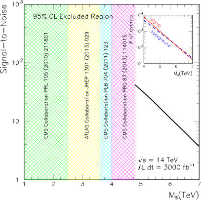
Figure 4: Signal-to-noise ratio of the lowest massive Regge excitations for the HL-LHC in the dijet (left) and $\gamma$ + jet (right) topologies. For comparison, we also show ATLAS and CMS upper limits on $M_{s}$ from unsuccessful searches of new particles decaying to pairs of partons (quarks, antiquarks, or gluons) [30, 31, 32, 33]. For LHC phase I, the signal-to-noise ratio is suppressed by $\simeq 0.32$.

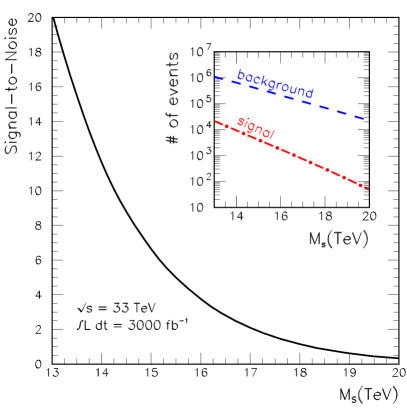
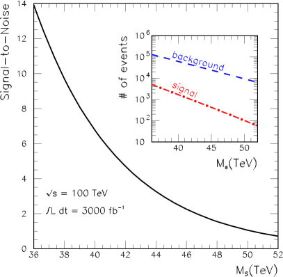
Figure 5: Dijet signal-to-noise ratio of the lowest massive Regge excitations for HE-LHC (left) and VLHC (right).

Excitations of the second massive string state may become visible at the HE-LHC and VLHC. The relevant resonant amplitudes around $s=2M_{s}$ are as follows:

$$\mathcal{M}(g_{1}^{-},g_{2}^{-},g_{3}^{+},g_{4}^{+}) = \frac{8g_{3}^{2}M_{s}^{2}\cos(\theta)}{s-2M_{s}^{2}}{\rm Tr}([T^{a_{1}},T^{a_{2}}][T^{a_{3}},T^{a_{4}}])$$ (6.4)

$$= -\frac{8g_{3}^{2}M_{s}^{2}}{s-2M_{s}^{2}}d^{1}_{0,0}(\theta)f^{a_{1}a_{2}a}f^{a_{3}a_{4}a}\,,$$

$$\mathcal{M}(g_{1}^{-},g_{2}^{+},g_{3}^{+},g_{4}^{-}) = -\frac{8g_{3}^{2}M_{s}^{2}}{s-2M_{s}^{2}}\left(\frac{1+\cos\theta}{2}\right)^{2}\cos\theta\leavevmode\nobreak\ f^{a_{1}a_{2}a}f^{a_{3}a_{4}a}$$ (6.5)

$$= -\frac{8g_{3}^{2}M_{s}^{2}}{s-2M_{s}^{2}}\left(\frac{1}{3}d^{3}_{+2,+2}(\theta)+\frac{2}{3}d^{2}_{+2,+2}(\theta)\right)f^{a_{1}a_{2}a}f^{a_{3}a_{4}a}\,,$$

$$\mathcal{M}(g_{1}^{-},g_{2}^{+},g_{3}^{-},g_{4}^{+}) = -\frac{8g_{3}^{2}M_{s}^{2}}{s-2M_{s}^{2}}\left(\frac{1-\cos\theta}{2}\right)^{2}\cos\theta\leavevmode\nobreak\ f^{a_{1}a_{2}a}f^{a_{3}a_{4}a}$$ (6.6)

$$= -\frac{8g_{3}^{2}M_{s}^{2}}{s-2M_{s}^{2}}\left(\frac{1}{3}d^{3}_{+2,-2}(\theta)-\frac{2}{3}d^{2}_{+2,-2}(\theta)\right)f^{a_{1}a_{2}a}f^{a_{3}a_{4}a}\,,$$

$$\mathcal{M}(q_{1}^{-},\bar{q}_{2}^{+},g_{3}^{-},g_{4}^{+})=\frac{4g_{3}^{2}M_{s}^{2}}{s-2M_{s}^{2}}\left(\frac{1}{3}\sqrt{\frac{2}{5}}d^{3}_{+2,+1}(\theta)+\frac{1}{6}d^{2}_{+2,+1}(\theta)\right)[T^{a_{3}},T^{a_{4}}]_{\alpha_{1}\alpha_{2}},$$ (6.7)

$$\mathcal{M}(q_{1}^{-},\bar{q}_{2}^{+},g_{3}^{+},g_{4}^{-})=\frac{4g_{3}^{2}M_{s}^{2}}{s-2M_{s}^{2}}\left(\frac{1}{3}\sqrt{\frac{2}{5}}d^{3}_{+2,-1}(\theta)-\frac{1}{6}d^{2}_{+2,-1}(\theta)\right)[T^{a_{3}},T^{a_{4}}]_{\alpha_{1}\alpha_{2}},$$ (6.8)

$$\mathcal{M}(q_{1}^{\pm},g_{2}^{\pm},\bar{q}_{3}^{\mp},g_{4}^{\mp})=-\frac{4g_{3}^{2}M_{s}^{2}}{s-2M_{s}^{2}}\biggl{[}\frac{1}{3}d^{J=1/2}_{\mp 1/2,\mp 1/2}(\theta)+\frac{2}{3}d^{J=3/2}_{\mp 1/2,\mp 1/2}(\theta)\biggr{]}\bigl{(}T^{a_{4}}T^{a_{2}}\bigr{)}_{\alpha_{3}\alpha_{1}}\,,$$ (6.9)

$$\mathcal{M}(q_{1}^{\pm},g_{2}^{\mp},\bar{q}_{3}^{\mp},g_{4}^{\pm})=-\frac{4g_{3}^{2}M_{s}^{2}}{s-2M_{s}^{2}}\biggl{[}\frac{3}{5}d^{J=3/2}_{\pm 3/2,\pm 3/2}(\theta)+\frac{2}{5}d^{J=5/2}_{\pm 3/2,\pm 3/2}(\theta)\biggr{]}\bigl{(}T^{a_{4}}T^{a_{2}}\bigr{)}_{\alpha_{3}\alpha_{1}}\,.$$ (6.10)

For phenomenological purposes, the poles need to be softened to a Breit–Wigner form. We can tell what the intermediate states are from the Wigner $d$ matrices and put in the corresponding total decay widths. After this is done, the contributions of the various channels to the dijet production are as follows:

$$|\mathcal{M}(gg\rightarrow gg)|^{2}=\frac{9g_{3}^{4}}{16M_{s}^{4}}\left[\leavevmode\nobreak\ \frac{4M_{s}^{4}(t-u)^{2}}{(s-2M_{s}^{2})^{2}+2(\Gamma_{G^{(2)}}^{J=1}M_{s})^{2}}+\frac{4}{9}\leavevmode\nobreak\ \frac{t^{4}-6t^{3}u+6t^{2}u^{2}-6tu^{3}+u^{4}}{(s-2M_{s}^{2})^{2}+2\Gamma_{G^{(2)}}^{J=3}\Gamma_{G^{(2)}}^{J=2}M_{s}^{2}}\right.$$

$$\left.+\frac{4}{9}\frac{t^{4}+u^{4}}{(s-2M_{s}^{2})^{2}+2(\Gamma_{G^{(2)}}^{J=2}M_{s})^{2}}+\frac{1}{36M_{s}^{4}}\frac{t^{6}-10t^{5}u+25t^{4}u^{2}+25t^{2}u^{4}-10tu^{5}+u^{6}}{(s-2M_{s}^{2})^{2}+2(\Gamma_{G^{(2)}}^{J=3}M_{s})^{2}}\right],$$ (6.11)

$$|\mathcal{M}(q\bar{q}\rightarrow gg)|^{2}=\frac{4g_{3}^{4}}{9M_{s}^{4}}\left[\frac{1}{6M_{s}^{4}}\leavevmode\nobreak\ \frac{tu(t^{4}-4t^{3}u+8t^{2}u^{2}-4tu^{3}+u^{4})}{(s-2M_{s}^{2})^{2}+2(\Gamma_{G^{(2)}}^{J=3}M_{s})^{2}}\right.$$

$$\left.+\frac{1}{6}\leavevmode\nobreak\ \frac{tu\left(t^{2}+u^{2}\right)}{(s-2M_{s}^{2})^{2}+2(\Gamma_{G^{(2)}}^{J=2}M_{s})^{2}}+\frac{2}{3}\leavevmode\nobreak\ \frac{tu\left(t^{2}-3tu+u^{2}\right)}{(s-2M_{s}^{2})^{2}+2\Gamma_{G^{(2)}}^{J=3}\Gamma_{G^{(2)}}^{J=2}M_{s}^{2}}\right]\,\,,$$ (6.12)

$$|\mathcal{M}(gg\rightarrow q\bar{q})|^{2}=\frac{g_{3}^{4}N_{f}}{16M_{s}^{4}}\left[\frac{1}{6M_{s}^{4}}\leavevmode\nobreak\ \frac{tu(t^{4}-4t^{3}u+8t^{2}u^{2}-4tu^{3}+u^{4})}{(s-2M_{s}^{2})^{2}+2(\Gamma_{G^{(2)}}^{J=3}M_{s})^{2}}\right.$$

$$\left.+\frac{1}{6}\leavevmode\nobreak\ \frac{tu\left(t^{2}+u^{2}\right)}{(s-2M_{s}^{2})^{2}+2(\Gamma_{G^{(2)}}^{J=2}M_{s})^{2}}+\frac{2}{3}\leavevmode\nobreak\ \frac{tu\left(t^{2}-3tu+u^{2}\right)}{(s-2M_{s}^{2})^{2}+2\Gamma_{G^{(2)}}^{J=3}\Gamma_{G^{(2)}}^{J=2}M_{s}^{2}}\right]\,,$$ (6.13)

$$\bigl{|}\mathcal{M}(q_{L}g\rightarrow q_{L}g)\bigr{|}^{2}=\bigl{|}\mathcal{M}(\bar{q}_{R}g\rightarrow\bar{q}_{R}g)\bigr{|}^{2}$$ (6.14)

$$= \frac{8g_{3}^{4}}{9M_{s}^{2}}\left\{\left[\frac{1}{9}\frac{-M_{s}^{4}u}{\left({s}-2M_{s}^{2}\right)^{2}+2\left(\Gamma^{J=1/2}_{Q^{(2)}_{L}}M_{s}\right)^{2}}+\frac{1}{9}\frac{-{u}(2{t}-{u})^{2}}{\left({s}-2M_{s}^{2}\right)^{2}+2\left(\Gamma^{J=3/2}_{\tilde{Q}^{(2)}_{L}}M_{s}\right)^{2}}\right]\right.$$

$$+ \frac{1}{4M_{s}^{4}}\left[\frac{9}{25}\frac{-M_{s}^{4}u^{3}}{\left({s}-2M_{s}^{2}\right)^{2}+2\left(\Gamma^{J=3/2}_{Q^{(2)}_{L}}M_{s}\right)^{2}}+\frac{1}{25}\frac{-{u}^{3}(4{t}-{u})^{2}}{\left({s}-2M_{s}^{2}\right)^{2}+2\left(\Gamma^{J=5/2}_{Q^{(2)}_{L}}M_{s}\right)^{2}}\right]$$

$$+ \left.\left[\frac{2}{9}\frac{M_{s}^{2}(-2tu+u^{2})}{\left({s}-2M_{s}^{2}\right)^{2}+2\Gamma^{J=1/2}_{Q^{(2)}_{L}}\Gamma^{J=3/2}_{\tilde{Q}^{(2)}_{L}}M_{s}^{2}}+\frac{3}{50}\frac{M_{s}^{-2}(-4{t}{u}^{3}+{u}^{4})}{\left({s}-2M_{s}^{2}\right)^{2}+2\Gamma^{J=3/2}_{Q^{(2)}_{L}}\Gamma^{J=5/2}_{Q^{(2)}_{L}}M_{s}^{2}}\right]\right\},$$

$$\bigl{|}\mathcal{M}(q_{R}g\rightarrow q_{R}g)\bigr{|}^{2}=\bigl{|}\mathcal{M}(\bar{q}_{L}g\rightarrow\bar{q}_{L}g)\bigr{|}^{2}$$ (6.15)

$$= \frac{8g_{3}^{4}}{9M_{s}^{2}}\left\{\left[\frac{1}{9}\frac{-M_{s}^{4}u}{\left({s}-2M_{s}^{2}\right)^{2}+2\left(\Gamma^{J=1/2}_{Q^{(2)}_{R}}M_{s}\right)^{2}}+\frac{1}{9}\frac{-{u}(2{t}-{u})^{2}}{\left({s}-2M_{s}^{2}\right)^{2}+2\left(\Gamma^{J=3/2}_{\tilde{Q}^{(2)}_{R}}M_{s}\right)^{2}}\right]\right.$$

$$+ \frac{1}{4M_{s}^{4}}\left[\frac{9}{25}\frac{-M_{s}^{4}u^{3}}{\left({s}-2M_{s}^{2}\right)^{2}+2\left(\Gamma^{J=3/2}_{Q^{(2)}_{R}}M_{s}\right)^{2}}+\frac{1}{25}\frac{-{u}^{3}(4{t}-{u})^{2}}{\left({s}-2M_{s}^{2}\right)^{2}+2\left(\Gamma^{J=5/2}_{Q^{(2)}_{R}}M_{s}\right)^{2}}\right]$$

$$+ \left.\left[\frac{2}{9}\frac{M_{s}^{2}(-2tu+u^{2})}{\left({s}-2M_{s}^{2}\right)^{2}+2\Gamma^{J=1/2}_{Q^{(2)}_{R}}\Gamma^{J=3/2}_{\tilde{Q}^{(2)}_{R}}M_{s}^{2}}+\frac{3}{50}\frac{M_{s}^{-2}(-4{t}{u}^{3}+{u}^{4})}{\left({s}-2M_{s}^{2}\right)^{2}+2\Gamma^{J=3/2}_{Q^{(2)}_{R}}\Gamma^{J=5/2}_{Q^{(2)}_{R}}M_{s}^{2}}\right]\right\},$$

The total decay widths for $n=2$ string resonances can be computed using the formulas in Table 4. We note that the widths of $Q^{(2)}$ are model dependent since they can decay into the $U(1)$ gauge bosons. In the $U(3)\times Sp(1)\times U(1)$ D-brane model, we have (at $M_{s}\sim 15$ TeV)

$$\Gamma_{G^{(2)}}^{J=3}=58\,(M_{s}/{\rm TeV})\leavevmode\nobreak\ {\rm GeV},\quad\Gamma_{G^{(2)}}^{J=2}=53\,(M_{s}/{\rm TeV})\leavevmode\nobreak\ {\rm GeV},$$

$$\Gamma_{G^{(2)}}^{J=1}=67\,(M_{s}/{\rm TeV})\leavevmode\nobreak\ {\rm GeV},\quad\Gamma_{Q^{(2)}_{L}}^{J=5/2}=30\,(M_{s}/{\rm TeV})\leavevmode\nobreak\ {\rm GeV},$$

$$\Gamma_{Q^{(2)}_{L}}^{J=3/2}=26\,(M_{s}/{\rm TeV})\leavevmode\nobreak\ {\rm GeV},\quad\Gamma_{\tilde{Q}^{(2)}_{L}}^{J=3/2}=38\,(M_{s}/{\rm TeV})\leavevmode\nobreak\ {\rm GeV}$$

$$\Gamma_{Q^{(2)}_{L}}^{J=1/2}=37\,(M_{s}/{\rm TeV})\leavevmode\nobreak\ {\rm GeV},\quad\Gamma_{Q^{(2)}_{R}}^{J=5/2}=26\,(M_{s}/{\rm TeV})\leavevmode\nobreak\ {\rm GeV}$$

$$\Gamma_{Q^{(2)}_{L}}^{J=3/2}=22\,(M_{s}/{\rm TeV})\leavevmode\nobreak\ {\rm GeV},\quad\Gamma_{\tilde{Q}^{(2)}_{L}}^{J=3/2}=32\,(M_{s}/{\rm TeV})\leavevmode\nobreak\ {\rm GeV}$$

$$\Gamma_{Q^{(2)}_{L}}^{J=1/2}=31\,(M_{s}/{\rm TeV})\leavevmode\nobreak\ {\rm GeV}\,.$$ (6.16)

At higher string scales, the decay widths slightly decrease because of the running of the couplings. For $M_{s}\sim 40$ TeV, we obtain

$$\Gamma_{G^{(2)}}^{J=3}=50\,(M_{s}/{\rm TeV})\leavevmode\nobreak\ {\rm GeV},\quad\Gamma_{G^{(2)}}^{J=2}=46\,(M_{s}/{\rm TeV})\leavevmode\nobreak\ {\rm GeV},$$

$$\Gamma_{G^{(2)}}^{J=1}=59\,(M_{s}/{\rm TeV})\leavevmode\nobreak\ {\rm GeV},\quad\Gamma_{Q^{(2)}_{R}}^{J=5/2}=27\,(M_{s}/{\rm TeV})\leavevmode\nobreak\ {\rm GeV},$$

$$\Gamma_{Q^{(2)}_{R}}^{J=3/2}=23\,(M_{s}/{\rm TeV})\leavevmode\nobreak\ {\rm GeV},\quad\Gamma_{\tilde{Q}^{(2)}_{R}}^{J=3/2}=34\,(M_{s}/{\rm TeV})\leavevmode\nobreak\ {\rm GeV}$$

$$\Gamma_{Q^{(2)}_{R}}^{J=1/2}=33\,(M_{s}/{\rm TeV})\leavevmode\nobreak\ {\rm GeV},\quad\Gamma_{Q^{(2)}_{R}}^{J=5/2}=23\,(M_{s}/{\rm TeV})\leavevmode\nobreak\ {\rm GeV}$$

$$\Gamma_{Q^{(2)}_{R}}^{J=3/2}=19\,(M_{s}/{\rm TeV})\leavevmode\nobreak\ {\rm GeV},\quad\Gamma_{\tilde{Q}^{(2)}_{R}}^{J=3/2}=28\,(M_{s}/{\rm TeV})\leavevmode\nobreak\ {\rm GeV}$$

$$\Gamma_{Q^{(2)}_{R}}^{J=1/2}=27\,(M_{s}/{\rm TeV})\leavevmode\nobreak\ {\rm GeV}\,.$$ (6.17)

The dijet signal-to-noise ratio for $n=2$ is shown in Fig. 6. For $M_{s}\lesssim 10.5\leavevmode\nobreak\ {\rm TeV}$ the second massive Regge excitations could also be observed with a statistical significance $\geq 5\sigma$ at the HE-LHC and for $M_{s}\lesssim 28\leavevmode\nobreak\ {\rm TeV}$ at the VLHC. Measurement of both resonant peaks would constitute definitive evidence for string physics.

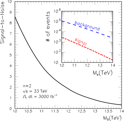
Figure 6: Dijet signal-to-noise ratio of $n=2$ Regge excitations for the HE-LHC (left) and VLHC (right).

6.2 Angular distributions

In what follows we briefly comment on the angular distributions. QCD parton-parton cross sections are dominated by $t$-channel exchanges that produce dijet angular distributions which peak at small center-of-mass scattering angles. In contrast, nonstandard contact interactions or excitations of resonances result in a more isotropic distribution. In terms of rapidity variable for standard transverse momentum cuts, dijets resulting from QCD processes will preferentially populate the large rapidity region, while the new processes generate events more uniformly distributed in the entire rapidity region. To analyze the details of the rapidity space the DØ Collaboration introduced a new parameter [109],

$$R=\frac{d\sigma/dM|_{(|y_{1}|,|y_{2}|<0.5)}}{d\sigma/dM|_{(0.5<|y_{1}|,|y_{2}|<1.0)}}\,,$$ (6.18)

the ratio of the number of events, in a given dijet mass bin, for both rapidities $|y_{1}|,|y_{2}|<0.5$ and both rapidities $0.5<|y_{1}|,|y_{2}|<1.0$. The ratio $R$ is a genuine measure of the most sensitive part of the angular distribution, providing a single number that can be measured as a function of the dijet invariant mass. An illustration of the use of this parameter in a heuristic model where standard model amplitudes are modified by a Veneziano form factor has been presented in Ref. [110].

It is important to note that although there are no $s$-channel resonances in $qq\rightarrow qq$ and $qq^{\prime}\rightarrow qq^{\prime}$ scattering, KK modes in the $t$ and $u$ channels generate calculable effective four-fermion contact terms. These in turn are manifest in a small departure from the QCD value of $R$ outside the resonant region [14]. In an optimistic scenario, measurements of this modification could shed light on the D-brane structure of the compact space. It could also serve to differentiate between a stringy origin for the resonance as opposed to an isolated structure such as a $Z^{\prime}$, which would not modify $R$ outside the resonant region. While the signal of quark scattering is suggestive, the analysis in Ref. [14] did not take into account all of the potential detector effects, which is necessary to be confident that the effect is real. In the next section we describe the first steps toward a more realistic description of the string physics processes.

7 SEGI

SEGI is a modification of the original BlackMax event generator [34, 35], which is extensively used by ATLAS and CMS collaborations in search for exotic physics. At its inception, BlackMax could simulate only black hole production in particle collisions (including all the greybody factors known to date) [111, 112, 113, 114, 115, 116, 117, 118]. Then it gradually grew into a very comprehensive generator that can accommodate different signatures of quantum gravity, e.g., stringball evaporation in a two-body final state [119]. With the current modification, BlackMax will be able to simulate production and decay of lowest massive Regge excitations yielding $\gamma$ + jet, $Z$ + jet, and dijet events.

A necessary input for the event generator is the amplitudes for perturbative string mediated processes. The parton-parton subprocesses of lowest massive Regge excitations decaying to dijets are given in Eqs. (3), (3.33), (3.36), and (3.37), whereas those decaying into $\gamma$ + jet are giving in Eqs. (3.41) and (3.42). The cross section can be written as a convolution of (6.2) with PDFs e.g., for dijets,

$$\sigma_{pp\to{\rm dijet}}=\sum_{ij}\int^{\hat{s}_{{\rm max}}/s}_{\hat{s}_{{\rm min}}/s}d\tau\int^{1}_{\tau}\frac{dx_{a}}{x_{a}}\ \sigma_{ij\to kl}\ f_{i}(x_{a},\hat{s})\ f_{j}(\tau/x_{a},\hat{s})\,,$$ (7.1)

where $\hat{s}_{\rm max}$ and $\hat{s}_{\rm min}$ are the maximum and minimum square center-of-mass energy of the colliding partons. The code iterates $10^{6}$ times to calculate the Monte Carlo integral. As an illustration, in Fig. 7 we show a comparison of the invariant mass distribution, setting $M_{s}=5\leavevmode\nobreak\ {\rm TeV}$, as obtained by SEGI and with the semianalytic (parton model) approach adopted in the preceding section.

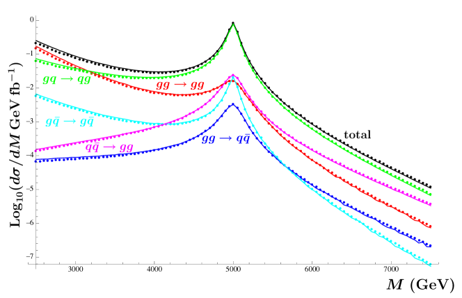
Figure 7: $d\sigma/dM$ vs. $M$ of first resonance string signal as obtained through the semianalytic parton model calculation (dots) and with SEGI (solid). We have taken $M_{s}=5\leavevmode\nobreak\ {\rm TeV}$.

The input parameters for the generator are read from the file parameter.txt (see Appendix D for how to access the file). In the following list we provide an explanation for the relevant input parameters:

• Number_of_simulations This parameter is the number of events to be generated.

• Type_of_incoming_particles This parameter determines the type of incoming particles:

  1. pp

  2. ${\tt p}\bar{\tt p}$

  3. e⁺e^-

• Center_of_mass_energy_of_incoming_particles This is the center-of-mass energy of the two incoming particles in units of GeV.

• Choose_a_case This parameter determines which type of events are simulated:

  1. nonrotating_black_hole_on_a_tensionless_brane

  2. nonrotating_black_hole_on_a_nonzero_tension_brane

  3. rotating_black_hole_on_a_tensionless_brane

  4. nonrotating_black_hole_with_fermion_tensionlees_brane_splitting

  5. stringballs_two_particle_final_states

  6. lowest_massive_Regge_excitations_decaying_to_dijets

  7. lowest_massive_Regge_excitations_decaying_to_gamma+jet

  8. lowest_massive_Regge_excitations_decaying_to_Z+jet

• Choose_a_pdf_file (200_to_240_CETQ6_or_$>$10000_for_LHAPDF) This parameter determines which PDF is used in the simulation. The code includes CETQ6 PDFs by default. In that case this parameter should be set from 200 to 240. For different PDFs one must install LHAPDF. The impact of the different PDFs and induced systematics in the production and decay of Regge recurrences is shown in Fig. 8.

• Minimum_mass This is the minimum mass that one wants to include in the simulation in units of GeV.

• Maximum_mass This is the maximum mass that one wants to include in the simulation in units of GeV.

• String_scale This parameter is the string scale $M_{s}$ in units of GeV.

• string_coupling This parameter is the string coupling; the default is set to $g_{s}=0.1$.

• kappa This is the $C-Y$mixing parameter; the default is set to $\kappa=0.14$.

All the other BlackMax parameters are irrelavant for simulation of Regge recurrences.

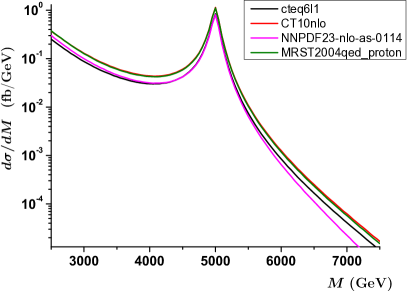
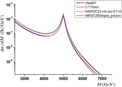
Figure 8: Systematic uncertainty of the dijet (left) and $\gamma$ + jet (right) string signal due to PDFs as obtained with SEGI.

The generator gives the output.txt file. This file contains the cross sections and the energy momentum distributions of the incoming and outgoing particles (pseudorapidity distributions are displayed in Fig. 9 for illustrative purposes only). The incoming particles are marked as parent. The outgoing particles are marked as elast. The meaning of each column is the same as in the original BlackMax event generator [34, 35]. The most up-to-date source code and TarBall can be downloaded from:

http://projects.hepforge.org/blackmax/

The details for SEGI installation can be found in the BlackMax manual [35]. For completness, a brief summary of the installation process is provided in Appendix D.

Thus far we have included in SEGI string excitations only up to $n=1$. In future versions we plan to extend the code to account for higher order excitations of the string, as well as $qq\to qq$ and $qq^{\prime}\to qq^{\prime}$ interactions.

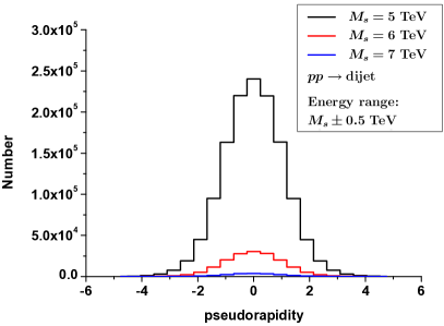
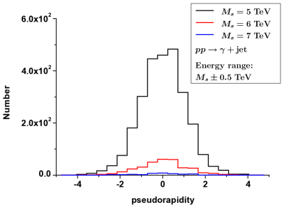
Figure 9: Dijet (left) and $\gamma$ + jet (right) pseudorapidity distributions.

8 Conclusions

We have explored the discovery potential of existing and proposed hadron colliders to unmask excitations of the string. We have studied the direct production of Regge recurrences, focusing on the first and second excited levels of open strings localized on the world volume of D-branes. In this framework, $U(1)_{B}$ and $SU(3)_{C}$ appear as subgroups of $U(3)$ associated with open strings ending on a stack of three D-branes. In addition, the minimal models contain two other stacks to accommodate the electroweak $SU(2)_{L}\subset U(2)$ and the hypercharge $U(1)_{Y}$. For such D-brane models, the resonant parts of the relevant string theory amplitudes are universal to leading order in the gauge coupling. As a consequence, it is feasible to extract genuine string effects which are independent of the compactification scheme. In this paper we have made use of the amplitudes evaluated near the first and second resonant poles to report on the discovery potential for Regge excitations of the quark, the gluon, and the color singlet living on the QCD stack of D-branes.

To calculate the string signal for $n=1$ resonances, we used the partial decay widths obtained elsewhere [7]. To compute the signal for $n=2$ resonances, we have presented here a complete calculation of all relevant decay widths of the second massive-level string states, including decays into massless particles and a massive $n=1$ and a massless particle. The latter were obtained from factorizing four-point amplitudes with one first massive-level string state computed in Ref. [11]. The partial decay widths of the spin-3 and spin-2 bosons from the second massive level were also obtained from direct string amplitude computations and match exactly with the results obtained from factorization. We also constructed the helicity wave functions of arbitrary higher spin massive boson.

Our phenomenological study among the various processes indicates that:

• For $M_{s}\lesssim 7.1\leavevmode\nobreak\ {\rm TeV}$, the HL-LHC will be able to discover (with statistical significance $>5\sigma$) the lowest massive Regge excitations in dijet events. For string scales as high as 6.1 TeV, observations of resonant structures in $pp\to\gamma$ + jet can provide interesting corroboration (with statistical significance $>5\sigma$) of low-mass-scale string physics.

• The dijet discovery potential exceedingly improves at the HE-LHC and VLHC. For $n=1$, the HE-LHC will be able to discover string excitations up to $M_{s}\approx 15\leavevmode\nobreak\ {\rm TeV}$, whereas the VLHC will attain $5\sigma$ discovery up to $M_{s}\approx 41\leavevmode\nobreak\ {\rm TeV}$. Moreover, for $n=2$, the HE-LHC will reach $5\sigma$ discovery for $M_{s}\lesssim 10.5\leavevmode\nobreak\ {\rm TeV}$, while the VLHC will be able to discover Regge excitations for $M_{s}\lesssim 28\leavevmode\nobreak\ {\rm TeV}$.

• Keeping only transverse $Z$’s and assuming that cross sections $\times$ branching into lepton pairs are large enough for complete reconstruction of $pp\to Z$ + jet, the D-brane contribution to the signal is suppressed relative to $pp\to\gamma$ + jet by a factor of $\tan^{2}\theta_{W}=0.29$. This differs radically from stringball evaporation in two-body final state. In such a case, emissions of $\gamma$ + jet and $Z$ + jet are comparable. The suppression of $Z$ +jet production, the origin of which lies in the particular structure of the D-brane model, will hold true for all the low-lying levels of the string.

Our calculations have been performed using a semianalytic parton model approach which is cross checked against an original software package. The string event generator interfaces with HERWIG and Pythia through BlackMax. The source code is publically available in the hepforge repository.

In summary, in this paper we have provided a concrete starting point for understanding the string physics potential of proposed machines that would collide protons at energies approaching the boundary of what (wo)mankind can daydream to achieve. The results presented herein will help to lay out opportunities, connections, and challenges for future LHC upgrades.

Appendix A Notation of group factors

We define the structure constant $f^{abc}$ and the total symmetric group factor $d^{abc}$ as

$$[T^{a},T^{b}] =i\sum_{c}f^{abc}T^{c}\,,$$ (A.1)

$$\{T^{a},T^{b}\} =4\sum_{c}d^{abc}T^{c}\,.$$ (A.2)

With the notation ${\rm Tr}(T^{a}T^{b})=\frac{1}{2}\delta^{ab}$, we could obtain

$${\rm Tr}([T^{a},T^{b}]T^{c}) =\tfrac{i}{2}f^{abc}\,,$$ (A.3)

$${\rm Tr}(\{T^{a},T^{b}\}T^{c}) =2d^{abc}\,.$$ (A.4)

We could also obtain

$${\rm Tr}(T^{ab}T^{cd})=2\sum_{e}{\rm Tr}(T^{ab}T^{e}){\rm Tr}(T^{cd}T^{e})\,,$$ (A.5)

where $T^{ab}$ or $T^{cd}$ presents either $[T^{a},T^{b}]$ or $\{T^{a},T^{b}\}$.

We thus arrive at

$${\rm Tr}([T^{a},T^{b}][T^{c},T^{d}]) =-\tfrac{1}{2}\sum_{e}f^{abe}f^{cde}\,,$$ (A.6)

$${\rm Tr}(\{T^{a},T^{b}\}\{T^{c},T^{d}\}) =8\sum_{e}d^{abe}d^{cde}\,,$$ (A.7)

$${\rm Tr}([T^{a},T^{b}]\{T^{c},T^{d}\}) =2i\sum_{e}f^{abe}d^{cde}\,.$$ (A.8)

Appendix B Spinor helicity formalism for massless fields

B.1 Helicity wave functions for massless spin-$\frac{1}{2}$ fermions

For massless spin-$\frac{1}{2}$ spinors, we use the notation following Ref. [11],

$$|i\rangle =|k_{i}\rangle=u_{+}(k_{i})=v_{-}(k_{i})=\binom{0}{k_{i}^{*\dot{a}}}\,,$$ (B.1)

$$|i] =|k_{i}]=u_{-}(k_{i})=v_{+}(k_{i})=\binom{k_{i,a}}{0}\,,$$ (B.2)

$$[i| =[k_{i}|=\bar{u}_{+}(k_{i})=\bar{v}_{-}(k_{i})=(k_{i}^{a},0)\,,$$ (B.3)

$$\langle i| =\langle k_{i}|=\bar{u}_{-}(k_{i})=\bar{v}_{+}(k_{i})=(0,k_{i,\dot{a}}^{*})\,,$$ (B.4)

where the momenta with spinor indices are two-component commutative spinors, which are defined by

$$P^{\dot{a}a}=p_{\mu}\bar{\sigma}^{\mu\dot{a}a}=-p^{*\dot{a}}p^{a}\,,$$ (B.5)

$$P_{a\dot{a}}=p_{\mu}\sigma_{a\dot{a}}^{\mu}=-p_{a}p_{\dot{a}}^{*}\,,$$ (B.6)

where $p^{*\dot{a}}=(p^{a})^{*}$ and $p_{\dot{a}}^{*}=(p_{a})^{*}$. Spinor indices could be raised (lowered) by $\varepsilon^{ab}$ ($\varepsilon_{ab}$) or $a,b$ with dots,

$$p^{a}=\varepsilon^{ab}p_{b}\,,\qquad p^{*\dot{a}}=\varepsilon^{\dot{a}\dot{b}}p_{\dot{b}}^{*}\,.$$ (B.7)

The spinor products are defined by

$$\langle pq\rangle=\langle p|q\rangle=\bar{u}_{-}(p)u_{+}(q)=p_{\dot{a}}^{*}q^{*\dot{a}}\,,$$ (B.8)

$${}[pq]=[p|q]=\bar{u}_{+}(p)u_{-}(q)=p^{a}q_{a}\,,$$ (B.9)

and we have the following relations:

$$[pq]=-[qp]\,,\qquad\langle pq\rangle=-\langle qp\rangle\,,\qquad\langle pp\rangle=[pp]=0\,,$$ (B.10)

$$\langle pq\rangle^{*}=[qp]\,,\qquad\langle pq\rangle[qp]=-2(p\cdot q)\,.$$ (B.11)

B.2 Helicity wave functions for massless spin-1 gauge boson

The gauge transformation for a spin-1 gauge boson reads $\epsilon^{\mu}\rightarrow\epsilon^{\mu}+\Lambda k^{\mu}$. The massless spin-1 gauge boson only has 2 degrees of freedom, which are helicity up ($+$) and down ($-$). The helicity wave functions (polarization vectors) of a massless spin-1 gauge boson can be written as

$$\epsilon_{\mu}^{+}(k,r) =\frac{\langle r|\gamma_{\mu}|k]}{\sqrt{2}\langle rk\rangle}=\frac{r_{\dot{a}}^{*}\bar{\sigma}_{\mu}^{\dot{a}a}k_{a}}{\sqrt{2}\langle rk\rangle}\,,$$ (B.12)

$$\epsilon_{\mu}^{-}(k,r) =-\frac{[r|\gamma_{\mu}|k\rangle}{\sqrt{2}[rk]}=-\frac{r^{a}\sigma_{\mu a\dot{a}}k^{*\dot{a}}}{\sqrt{2}[rk]}\,,$$ (B.13)

where $k$ is the momentum of the gauge boson and $r$ is the reference momentum which can be chosen to be any lightlike momentum except $k$. The final results of the helicity amplitudes are independent of the choice of reference momentum $r$.

Appendix C Helicity wave functions for massive spin-$\frac{1}{2}$ and -$\frac{3}{2}$ fermions

The wave functions of massive spin-$\frac{1}{2}$ and spin-$\frac{3}{2}$ fermions were constructed in Ref. [104].

C.1 Helicity wave functions for massive spin-$\frac{1}{2}$ fermions

Massive spin-$\frac{1}{2}$ fermions wave functions satisfy the Dirac equation

$$(\not{k}+m)u(k) =0\,,$$ (C.1)

$$(\not{k}-m)v(k) =0\,,$$ (C.2)

where $u(k)$ and $v(k)$ are positive and negative energy solutions with the momentum $k^{\mu}$, which correspond to fermion and antifermion wave functions, respectively. After decomposing $k$ into two lightlike momenta $p,q$, up to a phase factor, the helicity wave function of the massive spin-$\frac{1}{2}$ fermions can be written as

$$u_{+}(k)=\binom{\frac{\langle qp\rangle}{m}q_{a}}{p^{*\dot{a}}}\,,\qquad u_{-}(k)=\binom{p_{a}}{\frac{[qp]}{m}q^{*\dot{a}}}\,,$$ (C.3)

$$v_{+}(k)=\binom{p_{a}}{\frac{[pq]}{m}q^{*\dot{a}}}\,,\qquad v_{-}(k)=\binom{\frac{\langle pq\rangle}{m}q_{a}}{p^{*\dot{a}}}\,.$$ (C.4)

C.2 Massive spin-$\frac{3}{2}$ fermions wave functions

A massive spin-$\frac{3}{2}$ fermion could be described by Rarita–Schwinger spinor-vector $\Psi^{A,\mu}$ which satisfies equations

$$(i\not{\partial}-m)_{\phantom{A}B}^{A}\Psi^{B,\mu} =0\,,$$ (C.5)

$$(\gamma_{\mu})_{\phantom{A}B}^{A}\Psi^{B,\mu} =0\,,$$ (C.6)

$$\partial_{\mu}\Psi^{B,\mu} =0\,,$$ (C.7)

where $A$ and $B$ are spinor indices which run from 1 to 4. We can rewrite the first equation in terms of positive and negative solutions of Dirac equation, i.e., $U$ and $V$, which read

$$(\not{k}+m)_{\phantom{A}B}^{A}U(k)^{B,\mu} =0\,,$$ (C.8)

$$(\not{k}-m)_{\phantom{A}B}^{A}V(k)^{B,\mu} =0\,.$$ (C.9)

Using the same decomposition $k=p+q$, where $p,q$ are lightlike reference momenta, we have, up to a phase factor,

$$U^{A,\mu}(+\tfrac{3}{2}) =\frac{1}{\sqrt{2}m}\binom{\frac{\langle qp\rangle}{m}q_{a}}{p^{*\dot{a}}}(p_{\dot{b}}^{*}\bar{\sigma}^{\mu\dot{b}b}q_{b})\,,$$ (C.10)

$$U^{A,\mu}(+\tfrac{1}{2}) =\frac{\bar{\sigma}^{\mu\dot{b}b}}{\sqrt{6}m}\left[\binom{\frac{\langle qp\rangle}{m}q_{a}}{p^{*\dot{a}}}(p_{\dot{b}}^{*}p_{b}-q_{\dot{b}}^{*}q_{b})+\binom{\frac{\langle qp\rangle}{m}p_{a}}{-q^{*\dot{a}}}(p_{\dot{b}}^{*}q_{b})\right]\,,$$ (C.11)

$$U^{A,\mu}(-\tfrac{1}{2}) =\frac{\bar{\sigma}^{\mu\dot{b}b}}{\sqrt{6}m}\left[\binom{p_{a}}{\frac{[qp]}{m}q^{*\dot{a}}}(p_{\dot{b}}^{*}p_{b}-q_{\dot{b}}^{*}q_{b})+\binom{-q_{a}}{\frac{[qp]}{m}p^{*\dot{a}}}(q_{\dot{b}}^{*}p_{b})\right]\,,$$ (C.12)

$$U^{A,\mu}(-\tfrac{3}{2}) =\frac{1}{\sqrt{2}m}\binom{p_{a}}{\frac{[qp]}{m}q^{*\dot{a}}}(q_{\dot{b}}^{*}\bar{\sigma}^{\mu\dot{b}b}p_{b})\,,$$ (C.13)

and

$$V^{A,\mu}(+\tfrac{3}{2}) =\frac{1}{\sqrt{2}m}\binom{p_{a}}{\frac{[pq]}{m}q^{*\dot{a}}}(q_{\dot{b}}^{*}\bar{\sigma}^{\mu\dot{b}b}p_{b})\,,$$ (C.14)

$$V^{A,\mu}(+\tfrac{1}{2}) =\frac{\bar{\sigma}^{\mu\dot{b}b}}{\sqrt{6}m}\left[\binom{p_{a}}{\frac{[pq]}{m}q^{*\dot{a}}}(p_{\dot{b}}^{*}p_{b}-q_{\dot{b}}^{*}q_{b})+\binom{-q_{a}}{\frac{[pq]}{m}p^{*\dot{a}}}(q_{\dot{b}}^{*}p_{b})\right]\,,$$ (C.15)

$$V^{A,\mu}(-\tfrac{1}{2}) =\frac{\bar{\sigma}^{\mu\dot{b}b}}{\sqrt{6}m}\left[\binom{\frac{\langle pq\rangle}{m}q_{a}}{p^{*\dot{a}}}(p_{\dot{b}}^{*}p_{b}-q_{\dot{b}}^{*}q_{b})+\binom{\frac{\langle pq\rangle}{m}p_{a}}{-q^{*\dot{a}}}(p_{\dot{b}}^{*}q_{b})\right]\,,$$ (C.16)

$$V^{A,\mu}(-\tfrac{3}{2}) =\frac{1}{\sqrt{2}m}\binom{\frac{\langle pq\rangle}{m}q_{a}}{p^{*\dot{a}}}(p_{\dot{b}}^{*}\bar{\sigma}^{\mu\dot{b}b}q_{b})\,.$$ (C.17)

Appendix D SEGI installation

The first step is to download the zipped tar file which has to be unzipped to extract the files and make the program executable:

gunzip BlackMax-2.00.tar.gz
tar -xvf BlackMax-2.00.tar

Before compilation one has to check the compiler version of gcc by executing the command

gcc --version

which generates the output

gcc (GCC) 3.4.6 20060404 (Red Hat 3.4.6-10)
Copyright (C) 2006 Free Software Foundation, Inc.
...

This second step is required because the latest gcc compiler version (4.1.2) has changed the names of some system libraries needed to compile Fortran with C code. The download is configured to use gcc version 4. If an older gcc version (e.g. 3.4.6) is in operation, then one needs to modify the BlackMax Makefile. This can be accomplished by uncommenting the following lines in the Makefile

F77LIB =g2c
F77COMP=g77

After that SEGI is ready for compilation. There are three different ways to run SEGI: (i) standalone mode for which no additional libraries are required, (ii) accessing PDFs from LHAPDF, or (iii) accessing PDFs from LHAPDF and simultaneous hadronization from Pythia. In each case a different compilation/linking step is required to produce the executable. For all three options, the default format of the event output is the Les Houches Accord format [36]. This text file can be used as input into HERWIG and Pythia to hadronize the SEGI events.

D.1 Standalone mode

In this version the proton parton densities are taken from CTEQ6m which are packaged with BlackMax. After unpacking, the command:

gmake BlackMaxOnly

has to be executed and the file parameter.txt has to be modified to select one of the 41 CTEQ6m PDF sets that has been bundled with BlackMax, e.g.,

choose$\_$a$\_$pdf$\_$file(200$\_$to$\_$240$\_$cteq6)Or$\_>$10000$\_$for$\_$LHAPDF
200

After that, the executable can be run

BlackMax $>\&!$ out

D.2 LHAPDF

This version uses the proton parton densities from the LHAPDF library, which must be downloaded from

http://projects.hepforge.org/lhapdf/

Of course, one has to install the package in a directory with write permission. One can do this by specifying an installation directory (for additional information, the reader is referred to the LHAPDF manual). Then the BlackMax Makefile must be edited to insert the library locations. One has to verify that the ${\tt LD\_LIBRARY\_PATH}$ environment variable includes the location of the newly built LHAPDF library:

export ${\tt LD\_LIBRARY\_PATH=\$LD\_LIBRARY\_PATH:/data/rizvi/atlas/lhapdf-5.3.0/lhapdf/lib}$
export ${\tt LHAPATH=/data/rizvi/atlas/lhapdf-5.3.0/lhapdf/share/lhapdf/PDFsets}$

The next step is to select a valid PDF set in parameter.txt, e.g., the LHAPDF partons from the H1 PDF2000 fit of HERA data:

choose$\_$a$\_$pdf$\_$file(200$\_$to$\_$240$\_$cteq6_or$\_>$10000$\_$for$\_$LHAPDF)
70050

After unpacking the source files one can compile the program

gmake BlackMax

After that, the executable can be run

BlackMax $>\&!$ out

D.3 LHAPDF with simultaneous Pythia hadronization

To hadronize the events BlackMax comes with an interface to Pythia. To generate fully hadronized events one needs to download and install the latest versions of LHAPDF and PYTHIA. They are available at

http://www.hepforge.org/downloads/pythia6
and http://www.hepforge.org/downloads/lhapdf

BlackMax has been tested wth Pythia 6.4.10 and LHAPDF 5.3.0. After that, one has to create the Pythia libraries and remove both the following four dummy routines

upinit.f
upevnt.f
pdfset.f
structm.f

and the pdfset.f routine from the Pythia Makefile. The four routines above are all dummy routines which actually exist in LHAPDF. Next, one must edit the BlackMax Makefile to insert the library locations, while checking that the ${\tt LD\_LIBRARY\_PATH}$ environment variable includes the location of the newly built Pythia and LHAPDF libraries:

export ${\tt LD\_LIBRARY\_PATH=\$LD\_LIBRARY\_PATH:/data/rizvi/atlas/lhapdf-5.3.0/lhapdf/lib}$
export ${\tt LHAPATH=/data/rizvi/atlas/lhapdf-5.3.0/lhapdf/share/lhapdf/PDFsets}$

Finally, one has to create the BlackMax executable using the target “all” which will link to the Pythia and LHAPDF libraries,

gmake all

and select a valid PDF set in parameter.txt, e.g.,

${\tt choose\_a\_pdf\_file(200\_to\_240\_cteq6)Or\_>10000\_for\_LHAPDF}$
$10050$

After that, the exectuable can be run

BlackMax $>\&!$ out

References

- [1] I. Antoniadis, N. Arkani-Hamed, S. Dimopoulos and G. R. Dvali, Phys. Lett. B 436, 257 (1998) [hep-ph/9804398].
- [2] S. Chatrchyan et al. [CMS Collaboration], Phys. Lett. B 716, 30 (2012) [arXiv:1207.7235 [hep-ex]].
- [3] G. Aad et al. [ATLAS Collaboration], Phys. Lett. B 716, 1 (2012) [arXiv:1207.7214 [hep-ex]].
- [4] E. Accomando, I. Antoniadis and K. Benakli, Nucl. Phys. B 579, 3 (2000) [hep-ph/9912287].
- [5] L. A. Anchordoqui, H. Goldberg, S. Nawata and T. R. Taylor, Phys. Rev. Lett. 100, 171603 (2008) [arXiv:0712.0386 [hep-ph]].
- [6] L. A. Anchordoqui, H. Goldberg, S. Nawata and T. R. Taylor, Phys. Rev. D 78, 016005 (2008) [arXiv:0804.2013 [hep-ph]].
- [7] L. A. Anchordoqui, H. Goldberg and T. R. Taylor, Phys. Lett. B 668, 373 (2008) [arXiv:0806.3420 [hep-ph]].
- [8] L. A. Anchordoqui, H. Goldberg, D. Lüst, S. Nawata, S. Stieberger and T. R. Taylor, Phys. Rev. Lett. 101, 241803 (2008) [arXiv:0808.0497 [hep-ph]].
- [9] D. Lüst, S. Stieberger and T. R. Taylor, Nucl. Phys. B 808, 1 (2009) [arXiv:0807.3333 [hep-th]].
- [10] D. Lüst, O. Schlotterer, S. Stieberger and T. R. Taylor, Nucl. Phys. B 828, 139 (2010) [arXiv:0908.0409 [hep-th]].
- [11] W. -Z. Feng, D. Lüst, O. Schlotterer, S. Stieberger and T. R. Taylor, Nucl. Phys. B 843, 570 (2011) [arXiv:1007.5254 [hep-th]].
- [12] W. -Z. Feng and T. R. Taylor, Nucl. Phys. B 856, 247 (2012) [arXiv:1110.1087 [hep-th]].
- [13] W. -Z. Feng, D. Lüst and O. Schlotterer, Nucl. Phys. B 861, 175 (2012) [arXiv:1202.4466 [hep-th]].
- [14] L. A. Anchordoqui, H. Goldberg, D. Lüst, S. Nawata, S. Stieberger and T. R. Taylor, Nucl. Phys. B 821, 181 (2009) [arXiv:0904.3547 [hep-ph]].
- [15] L. A. Anchordoqui, H. Goldberg, D. Lüst, S. Stieberger and T. R. Taylor, Mod. Phys. Lett. A 24, 2481 (2009) [arXiv:0909.2216 [hep-ph]].
- [16] L. A. Anchordoqui, W. -Z. Feng, H. Goldberg, X. Huang and T. R. Taylor, Phys. Rev. D 83, 106006 (2011) [arXiv:1012.3466 [hep-ph]].
- [17] S. Cullen, M. Perelstein and M. E. Peskin, Phys. Rev. D 62, 055012 (2000) [hep-ph/0001166].
- [18] P. Burikham, T. Han, F. Hussain and D. W. McKay, Phys. Rev. D 69, 095001 (2004) [hep-ph/0309132].
- [19] P. Burikham, T. Figy and T. Han, Phys. Rev. D 71, 016005 (2005) [Erratum-ibid. D 71, 019905 (2005)] [hep-ph/0411094].
- [20] M. Chemtob, Phys. Rev. D 78, 125020 (2008) [arXiv:0808.1242 [hep-ph]].
- [21] N. Kitazawa, JHEP 1010, 051 (2010) [arXiv:1008.4989 [hep-ph]].
- [22] Z. Dong, T. Han, M. -x. Huang and G. Shiu, JHEP 1009, 048 (2010) [arXiv:1004.5441 [hep-ph]].
- [23] M. Hashi and N. Kitazawa, JHEP 1202, 050 (2012) [Erratum-ibid. 1204, 011 (2012)] [arXiv:1110.3976 [hep-ph]].
- [24] M. Hashi and N. Kitazawa, JHEP 1303, 127 (2013) [arXiv:1212.5372 [hep-ph]].
- [25] E. Dudas and J. Mourad, Nucl. Phys. B 575, 3 (2000) [hep-th/9911019].
- [26] D. Chialva, R. Iengo and J. G. Russo, Phys. Rev. D 71, 106009 (2005) [hep-ph/0503125].
- [27] B. Hassanain, J. March-Russell and J. G. Rosa, JHEP 0907, 077 (2009) [arXiv:0904.4108 [hep-ph]].
- [28] M. Perelstein and A. Spray, JHEP 0910, 096 (2009) [arXiv:0907.3496 [hep-ph]].
- [29] L. A. Anchordoqui, H. Goldberg, X. Huang and T. R. Taylor, Phys. Rev. D 82, 106010 (2010) [arXiv:1006.3044 [hep-ph]].
- [30] V. Khachatryan et al. [CMS Collaboration], Phys. Rev. Lett. 105, 211801 (2010) [arXiv:1010.0203 [hep-ex]].
- [31] G. Aad et al. [ATLAS Collaboration], JHEP 1301, 029 (2013) [arXiv:1210.1718 [hep-ex]].
- [32] S. Chatrchyan et al. [CMS Collaboration], Phys. Lett. B 704, 123 (2011) [arXiv:1107.4771 [hep-ex]].
- [33] S. Chatrchyan et al. [CMS Collaboration], Phys. Rev. D 87, 114015 (2013) [arXiv:1302.4794 [hep-ex]].
- [34] D. C. Dai, G. Starkman, D. Stojkovic, C. Issever, E. Rizvi and J. Tseng, Phys. Rev. D 77, 076007 (2008) [arXiv:0711.3012 [hep-ph]].
- [35] D. -C. Dai, C. Issever, E. Rizvi, G. Starkman, D. Stojkovic and J. Tseng, arXiv:0902.3577 [hep-ph].
- [36] E. Boos et al., arXiv:hep-ph/0109068.
- [37] Y. Gershtein et al., arXiv:1311.0299 [hep-ex].
- [38] https://indico.cern.ch/event/282344/. Future Circular Collider Study Kick-Off meeting.
- [39] http://indico.ihep.ac.cn/conferenceDisplay.py?confId=3813. Workshop on Future High Energy Circular Colliders.
- [40] P. A. R. Ade et al. [BICEP2 Collaboration], Phys. Rev. Lett. 112, 241101 (2014) [arXiv:1403.3985 [astro-ph.CO]].
- [41] H. Liu, P. Mertsch and S. Sarkar, Astrophys. J. 789, L29 (2014) [arXiv:1404.1899 [astro-ph.CO]].
- [42] R. Flauger, J. C. Hill and D. N. Spergel, arXiv:1405.7351 [astro-ph.CO].
- [43] R. Blumenhagen, B. Körs, D. Lüst, T. Ott, Nucl. Phys. B 616, 3 (2001) [hep-th/0107138].
- [44] M. Cvetic, G. Shiu and A. M. Uranga, Phys. Rev. Lett. 87, 201801 (2001) [arXiv:hep-th/0107143].
- [45] M. Cvetic, G. Shiu and A. M. Uranga, Nucl. Phys. B 615, 3 (2001) [arXiv:hep-th/0107166].
- [46] I. Antoniadis, E. Kiritsis and T. Tomaras, Fortsch. Phys. 49, 573 (2001) [arXiv:hep-th/0111269].
- [47] L. E. Ibanez, F. Marchesano and R. Rabadan, JHEP 0111, 002 (2001) [arXiv:hep-th/0105155].
- [48] E. Kiritsis and P. Anastasopoulos, JHEP 0205, 054 (2002) [arXiv:hep-ph/0201295].
- [49] D. Cremades, L. E. Ibanez and F. Marchesano, JHEP 0307, 038 (2003) [arXiv:hep-th/0302105].
- [50] G. Honecker, T. Ott, Phys. Rev. D 70, 126010 (2004) [hep-th/0404055].
- [51] F. Gmeiner, R. Blumenhagen, G. Honecker, D. Lüst and T. Weigand, JHEP 0601, 004 (2006) [arXiv:hep-th/0510170].
- [52] F. Gmeiner, G. Honecker, JHEP 0807, 052 (2008) [arXiv:0806.3039 [hep-th]].
- [53] E. Kiritsis, Phys. Rept. 421, 105 (2005) [Erratum-ibid. 429, 121 (2006)] [Fortsch. Phys. 52, 200 (2004)] [arXiv:hep-th/0310001].
- [54] R. Blumenhagen, M. Cvetic, P. Langacker and G. Shiu, Ann. Rev. Nucl. Part. Sci. 55, 71 (2005) [arXiv:hep-th/0502005].
- [55] R. Blumenhagen, B. Körs, D. Lüst, S. Stieberger, Phys. Rept. 445, 1 (2007) [hep-th/0610327].
- [56] G. Honecker and W. Staessens, PoS Corfu 2012, 107 (2013) [arXiv:1303.6845 [hep-th]].
- [57] D. Berenstein, arXiv:1401.4491 [hep-th].
- [58] M. Cvetic, J. Halverson and P. Langacker, JHEP 1111, 058 (2011) [arXiv:1108.5187 [hep-ph]].
- [59] W. -Z. Feng, G. Shiu, P. Soler and F. Ye, JHEP 1405, 065 (2014) [arXiv:1401.5890 [hep-ph]].
- [60] W. -Z. Feng, G. Shiu, P. Soler and F. Ye, arXiv:1401.5880 [hep-ph].
- [61] L. A. Anchordoqui, I. Antoniadis, H. Goldberg, X. Huang, D. Lüst and T. R. Taylor, Phys. Rev. D 85, 086003 (2012) [arXiv:1107.4309 [hep-ph]].
- [62] D. M. Ghilencea, L. E. Ibanez, N. Irges and F. Quevedo, JHEP 0208, 016 (2002) [arXiv:hep-ph/0205083].
- [63] L. A. Anchordoqui, I. Antoniadis, H. Goldberg, X. Huang, D. Lüst, T. R. Taylor and B. Vlcek, Phys. Rev. D 86, 066004 (2012) [arXiv:1206.2537 [hep-ph]].
- [64] L. A. Anchordoqui, I. Antoniadis, H. Goldberg, X. Huang, D. Lüst, T. R. Taylor and B. Vlcek, JHEP 1302, 074 (2013) [arXiv:1208.2821 [hep-ph]].
- [65] J. Erler, P. Langacker, S. Munir and E. Rojas, JHEP 0908, 017 (2009) [arXiv:0906.2435 [hep-ph]].
- [66] S. Schael et al. [ALEPH Collaboration, DELPHI Collaboration, L3 Collaboration, OPAL Collaboration, SLD Collaboration, LEP Electroweak Working Group, and SLD Electroweak and Heavy Flavour Groups], Phys. Rept. 427, 257 (2006) [arXiv:hep-ex/0509008].
- [67] M. S. Carena, A. Daleo, B. A. Dobrescu and T. M. P. Tait, Phys. Rev. D 70, 093009 (2004) [hep-ph/0408098].
- [68] E. Accomando, A. Belyaev, L. Fedeli, S. F. King and C. Shepherd-Themistocleous, Phys. Rev. D 83, 075012 (2011) [arXiv:1010.6058 [hep-ph]].
- [69] S. Chatrchyan et al. [CMS Collaboration], Phys. Lett. B 714, 158 (2012) [arXiv:1206.1849 [hep-ex]].
- [70] B. A. Dobrescu and F. Yu, Phys. Rev. D 88, 035021 (2013) [arXiv:1306.2629 [hep-ph]].
- [71] I. Antoniadis, E. Kiritsis and T. N. Tomaras, Phys. Lett. B 486, 186 (2000) [arXiv:hep-ph/0004214].
- [72] I. Antoniadis and S. Dimopoulos, Nucl. Phys. B 715, 120 (2005) [arXiv:hep-th/0411032].
- [73] D. Berenstein and S. Pinansky, Phys. Rev. D 75, 095009 (2007) [hep-th/0610104].
- [74] M. B. Green and J. H. Schwarz, Phys. Lett. B 149, 117 (1984).
- [75] E. Witten, Phys. Lett. B 149, 351 (1984).
- [76] M. Dine, N. Seiberg and E. Witten, Nucl. Phys. B 289, 589 (1987).
- [77] J. J. Atick, L. J. Dixon and A. Sen, Nucl. Phys. B 292, 109 (1987).
- [78] W. Lerche, B. E. W. Nilsson, A. N. Schellekens and N. P. Warner, Nucl. Phys. B 299, 91 (1988).
- [79] A. Sagnotti, Phys. Lett. B 294, 196 (1992) [hep-th/9210127].
- [80] J. Beringer et al. [Particle Data Group Collaboration], Phys. Rev. D 86, 010001 (2012).
- [81] D. Berenstein, R. Martinez, F. Ochoa and S. Pinansky, Phys. Rev. D 79, 095005 (2009) [arXiv:0807.1126].
- [82] I. Antoniadis, E. Kiritsis, J. Rizos and T. N. Tomaras, Nucl. Phys. B 660, 81 (2003) [arXiv:hep-th/0210263].
- [83] P. Anastasopoulos, T. P. T. Dijkstra, E. Kiritsis and A. N. Schellekens, Nucl. Phys. B 759, 83 (2006) [arXiv:hep-th/0605226].
- [84] L. A. Anchordoqui, H. Goldberg, X. Huang, D. Lüst and T. R. Taylor, Phys. Lett. B 701, 224 (2011) [arXiv:1104.2302 [hep-ph]].
- [85] L. A. Anchordoqui and H. Goldberg, Phys. Rev. Lett. 108, 081805 (2012) [arXiv:1111.7264 [hep-ph]].
- [86] I. Antoniadis, E. Kiritsis and J. Rizos, Nucl. Phys. B 637, 92 (2002) [arXiv:hep-th/0204153].
- [87] P. Anastasopoulos, JHEP 0308, 005 (2003) [arXiv:hep-th/0306042].
- [88] K. R. Dienes, C. F. Kolda and J. March-Russell, Nucl. Phys. B 492, 104 (1997) [arXiv:hep-ph/9610479].
- [89] G. Honecker, M. Ripka and W. Staessens, Nucl. Phys. B 868, 156 (2013) [arXiv:1209.3010 [hep-th]].
- [90] G. Honecker and W. Staessens, Fortsch. Phys. 62, 115 (2014) [arXiv:1312.4517 [hep-th]].
- [91] S. A. Abel, M. D. Goodsell, J. Jaeckel, V. V. Khoze and A. Ringwald, JHEP 0807, 124 (2008) [arXiv:0803.1449 [hep-ph]].
- [92] S. J. Parke and T. R. Taylor, Phys. Rev. Lett. 56, 2459 (1986).
- [93] S. Stieberger and T. R. Taylor, Phys. Rev. Lett. 97, 211601 (2006) [hep-th/0607184].
- [94] S. Stieberger and T. R. Taylor, Phys. Rev. D 74, 126007 (2006) [hep-th/0609175].
- [95] M. L. Mangano and S. J. Parke, Phys. Rept. 200, 301 (1991) [arXiv:hep-th/0509223].
- [96] L. J. Dixon, arXiv:hep-ph/9601359.
- [97] G. Veneziano, Nuovo Cim. A 57, 190 (1968).
- [98] T. van Ritbergen, A. N. Schellekens and J. A. M. Vermaseren, Int. J. Mod. Phys. A 14, 41 (1999) [arXiv:hep-ph/9802376].
- [99] G. T. Horowitz and J. Polchinski, Phys. Rev. D 55, 6189 (1997) [hep-th/9612146].
- [100] L. E. Ibanez and F. Quevedo, JHEP 9910, 001 (1999) [hep-ph/9908305].
- [101] M. Berasaluce-Gonzalez, L. E. Ibanez, P. Soler and A. M. Uranga, JHEP 1112, 113 (2011) [arXiv:1106.4169 [hep-th]].
- [102] P. Anastasopoulos, M. Cvetic, R. Richter and P. K. S. Vaudrevange, JHEP 1303, 011 (2013) [arXiv:1211.1017 [hep-th]].
- [103] G. Honecker and W. Staessens, JHEP 1310, 146 (2013) [arXiv:1303.4415 [hep-th]].
- [104] S. F. Novaes and D. Spehler, Nucl. Phys. B 371, 618 (1992).
- [105] D. Spehler and S. F. Novaes, Phys. Rev. D 44, 3990 (1991).
- [106] G. Aad et al. [ATLAS Collaboration], Phys. Lett. B 728, 562 (2014) [arXiv:1309.3230 [hep-ex]].
- [107] J. Pumplin, D. R. Stump, J. Huston, H. L. Lai, P. M. Nadolsky and W. K. Tung, JHEP 0207, 012 (2002) [hep-ph/0201195].
- [108] V. Khachatryan et al. [CMS Collaboration], arXiv:1406.5171 [hep-ex].
- [109] B. Abbott et al. [D0 Collaboration], Phys. Rev. Lett. 82, 2457 (1999) [arXiv:hep-ex/9807014].
- [110] P. Meade and L. Randall, JHEP 0805, 003 (2008) [arXiv:0708.3017 [hep-ph]].
- [111] T. Banks and W. Fischler, hep-th/9906038.
- [112] S. Dimopoulos and G. L. Landsberg, Phys. Rev. Lett. 87, 161602 (2001) [hep-ph/0106295].
- [113] S. B. Giddings and S. D. Thomas, Phys. Rev. D 65, 056010 (2002) [hep-ph/0106219].
- [114] P. Kanti and J. March-Russell, Phys. Rev. D 67, 104019 (2003) [hep-ph/0212199].
- [115] L. A. Anchordoqui, J. L. Feng, H. Goldberg and A. D. Shapere, Phys. Lett. B 594, 363 (2004) [hep-ph/0311365].
- [116] D. Stojkovic, Phys. Rev. Lett. 94, 011603 (2005) [hep-ph/0409124].
- [117] D. -C. Dai, G. D. Starkman and D. Stojkovic, Phys. Rev. D 73, 104037 (2006) [hep-ph/0605085].
- [118] S. Creek, O. Efthimiou, P. Kanti and K. Tamvakis, Phys. Rev. D 76, 104013 (2007) [arXiv:0707.1768 [hep-th]].
- [119] S. Dimopoulos and R. Emparan, Phys. Lett. B 526, 393 (2002) [hep-ph/0108060].