Additive Models for Conditional Bivariate Copulas: A Bayesian Approach

Abstract

Conditional copulas are flexible statistical tools that couple joint conditional and marginal conditional distributions. In a linear regression setting with more than one covariate and two dependent outcomes, we propose the use of additive models for conditional bivariate copula models and discuss computation and model selection tools for performing Bayesian inference. The method is illustrated using simulations and a real example.

Keywords: Additive models, Bayesian inference, Cross-validated marginal likelihood, Conditional copulas, Cubic splines, Markov chain Monte Carlo.

1 Introduction

Starting with the seminal paper of Sklar (1959), copulas have developed into an important tool used for modelling dependence in statistical models. If $Y_{1},Y_{2},\ldots,Y_{k}$ are continuous random variables with joint distribution function $H$ and marginal distributions $F_{1},F_{2},\ldots,F_{k}$, the unique copula $C:[0,1]^{k}\to[0,1]$ “couples” the joint and the marginal distributions via $H(y_{1},\ldots,y_{k})=C\{F_{1}(y_{1}),\ldots F_{n}(y_{k})\}$, for all $(y_{1},\ldots,y_{k})\in\mathbb{R}^{k}$. Therefore, in order to define $H$, we need the marginals $F_{i}$ and the copula $C$. This can be convenient in situations in which one has a good grasp on the marginal distributions.

As a natural extension, conditional copulas couple joint conditional and marginal conditional distributions (Lambert and Vandenhende, 2002; Patton, 2006). Specifically, if $X\in{\bf R}^{p}$ is a covariate vector, then

$$H_{X}(y_{1},\ldots,y_{k}\mid X)=C\{F_{1\mid X}(y_{1}\mid X),\ldots,F_{n\mid X}(y_{k}\mid X)\mid X\},\quad\mbox{for all}\;(y_{1},\ldots,y_{k})\in{\bf R}^{k}.$$ (1)

Conditional copulas models play an essential part in modelling high dimensional data. For instance, consider $X=(X_{1},\ldots,X_{4})\in{\bf R}^{4}$. Using a similar decomposition to the one used by Acar et al. (2012) (equation (3) at page 75) we can show that its four-dimensional continuous density $f(x):=f(x_{1},x_{2},x_{3},x_{4})$ can be decomposed as

$$f(x_{1},x_{2},x_{3},x_{4}) = f_{1}(x_{1})f_{2}(x_{2})f_{3}(x_{3})f_{4}(x_{4})$$ (2)

$$\times c_{12}\{F_{1}(x_{1}),F_{2}(x_{2})\}c_{23}\{F_{2}(x_{2}),F_{3}(x_{3})\}c_{14}\{F_{1}(x_{1}),F_{4}(x_{4})\}$$

$$\times c_{13\mid 2}\{F_{1\mid 2}(x_{1}|x_{2}),F_{3\mid 2}(x_{3}|x_{2})\}c_{24\mid 1}\{F_{2\mid 1}(x_{2}|x_{1}),F_{4\mid 1}(x_{4}|x_{1})\}$$

$$\times c_{43\mid 12}\{F_{4\mid 12}(x_{4}\mid x_{1},x_{2}),F_{3\mid 12}(x_{3}\mid x_{1},x_{2})\},$$

where, if ${\cal A},{\cal B}\subset\{1,2,3,4\}$ are set of indices and we have used the following notations: $f_{{\cal A}}$, $F_{{\cal A}}$ are, respectively, the joint density and distribution function of $\{X_{j}:j\in{\cal A}\}$; $f_{{\cal A}\mid{\cal B}}$, $F_{{\cal A}\mid{\cal B}}$ are the conditional density and distribution functions of $\{X_{j}:j\in{\cal A}\}$ given $\{X_{h}:h\in{\cal B}\}$; $c_{{\cal A}}$ and $c_{{\cal A}\mid{\cal B}}$ denote, respectively, the copula density for $\{X_{j}:j\in{\cal A}\}$ and the conditional copula density of $\{X_{j}:j\in{\cal A}\}$ given $\{X_{h}:h\in{\cal B}\}$. Not surprisingly, increasing the dimension of $X$ will result in a decomposition like (2) where we need to condition on more than two random variables. Acar et al. (2012) have shown that when replacing the conditional copulas with unconditional ones in (2), we are likely to incur inferential losses in terms of both bias and efficiency.

The conditional copula can also be a useful modelling tool in regression settings in which we observe outcomes $Y_{1},\ldots,Y_{k}$ along with covariate vector $X\in{\bf R}^{p}$ and of interest is not only the effect of the covariate on each response, but also the effect of $X$ on the dependence structure between the responses. Throughout the paper we consider parametric copula families in which the function $C$ assumes a parametric form indexed by a copula parameter $\theta$. In many applications one can reasonably assume that $\theta$ will vary with $X$. However, it is generally difficult to guess the functional relationship between $\theta$ and the covariate vector $X$ so its estimation requires flexible models that can capture a wide variety of patterns. This naturally leads to the use of semiparametric (Acar et al., 2011; Craiu and Sabeti, 2012) and nonparametric inferential tools (Omelka et al., 2009; Veraverbeke et al., 2011; Abegaz et al., 2012). As the dimension $p$ of the covariate vector $X$ increases, the volume of data required to keep the error within reasonable bounds increases very quickly (Abegaz et al., 2012). However, the generic examples discussed above motivate our search for practical inferential procedures for conditional copula models when $p>1$. The paper is developed situations in which the parameter $\theta$ is a scalar and there are two (i.e. $k=2$) continuous outcomes of interest, $Y_{1}$ and $Y_{2}$, that are marginally linked to the vector of covariates via linear regression models.

We propose here the use of additive models for studying the functional dependence between the covariate vector and the copula parameter. In this paper we will improve on the statistical ingredients developed by Craiu and Sabeti (2012) in two directions. Most importantly, we will examine the performance of their Bayesian cubic spline estimator within an additive model framework. Secondly, we investigate the performance of the cross validated marginal likelihood (CVML) criterion that adapts the seminal concept of cross-validation for marginal likelihood considered by Geisser and Eddy (1979) to the conditional copula setting.

In the next section we introduce the statistical model, describe the computational algorithms needed for inference and the calculation of the CVML criterion. Simulations and a real data analysis are discussed in Section 3. The paper closes with a discussion of future research directions.

2 The Model

In a regression setting we consider the continuous bivariate outcome $Y_{1},Y_{2}$ along with covariate $X\in{\bf R}^{p}$. Marginally, each response $Y_{i}$, $i=1,2$ is modelled using a normal regression model. For a sample of size $n$, $\{(Y_{1j},Y_{2j},X_{j}):\;1\leq j\leq n\}$, where $X_{j}=(X_{j1},\ldots,X_{jp})^{T}$, we assume marginally

$$Y_{ij}\sim N(X_{j}^{T}\beta_{i},\sigma_{i}^{2}),\;\forall 1\leq i\leq 2,\;1\leq j\leq n,$$ (3)

and joint density

$$f(Y_{1j},Y_{2j}|X_{j}) = \prod_{i=1}^{2}{1\over\sigma_{i}}\phi\left({Y_{ij}-X_{j}^{T}\beta_{i}\over\sigma_{i}}\right)\times$$

$$\times c^{(1,1)}\left\{\Phi\left({Y_{1j}-X_{j}^{T}\beta_{1}\over\sigma_{1}}\right),\Phi\left({Y_{2j}-X_{j}^{T}\beta_{2}\over\sigma_{2}}\right)\bigg{|}\theta(X_{j})\right\},\;\forall 1\leq j\leq n,$$

where $c^{(a,b)}(u,v|\theta)={\partial^{a+b}C(u,v|\theta)/\partial u^{a}\partial v^{b}}$, for all $0\leq a,b\leq 1$.

An important part of the model is the specification of $\theta(X)$. Many copula families have their parameter $\theta$ restricted to a subset of ${\bf R}$. In such cases we transform the parameter $\theta$ via a user-specified link function $g$ that maps the support of the copula parameter onto the real line and then we set $g(\theta)=\eta(X)$, where $\eta:{\bf R}^{p}\rightarrow{\bf R}$ is the unknown calibration function we want to estimate. It is known that there is a one-to-one correspondence between the copula parameter $\theta(X)$ and the conditional Kendall’s tau $\tau(X)=4{\rm E}\{H(Y_{1},Y_{2}|X)|X\}-1$ where the mean is taken with respect to the joint conditional density of $(Y_{1},Y_{2})$ given $X$. Therefore, one can parametrize the model on the $\tau$ or $\theta$ scale. In this paper the inference is performed directly on the copula parameter calibration function for computational convenience. However, when goodness-of-fit measures are reported across different copula families, it is recommended to use the $\tau$ scale which is parametrization invariant (see also discussion in Acar et al., 2011).

When $p>1$ we adopt an additive model (Hastie and Tibshirani, 1990) for $\eta(X)$

$$\eta(X)=\alpha_{0}+\sum_{i=1}^{p}\eta_{i}(X_{i}),$$ (4)

where $\alpha_{0}\in{\bf R}$ and each $\eta_{i}:{\bf R}\rightarrow{\bf R}$ is specified using the flexible cubic spline model suggested by Smith and Kohn (1996) in which

$$\eta_{i}(X_{i})=\sum_{j=1}^{3}{\alpha}_{j}^{(i)}X_{i}^{j}+\sum_{k=1}^{K^{(i)}}{\psi}_{k}^{(i)}{(X_{i}-{\gamma}_{k}^{(i)})^{3}}_{+}$$ (5)

and $a_{+}=\max(0,a)$. It is well known that the performance of spline-based estimators are influenced by the location of the knots $\gamma_{k}^{(i)}$. In our model this choice is automatic and data-driven.

A general remark is that in our implementations we assume that the covariates are independent random variables. In order to test this assumption when applying the method to real data, we have used tests based on the empirical copula process (Genest and Remillard, 2004; Kojadinovic and Holmes, 2009) and correlation of distances (Székely et al., 2007).

The priors assigned to the parameters involved in the marginal models are:

$$\beta_{i} \sim N(0,\sigma_{i}^{2}{\bf I}_{p}),\;\forall i=1,2$$

$$\sigma_{i}^{2} \sim IG(0.1,0.1),\;\forall i=1,2.$$

For the parameters involved in the cubic spline we follow the prior specifications used by Craiu and Sabeti (2012). For each covariate $X_{i}$, we select a fixed value for the maximum number of knots, $K_{\max}^{(i)}$. In the absence of additional information regarding which covariates are more likely to induce changes in $\eta$, we use the same $K_{\max}$ value for each $i=1,2,\ldots,p$. The range spanned by the observed values of covariate $X_{i}$ is divided into $K_{\max}^{(i)}$ intervals of equal length, $I_{1}^{(i)},\ldots,I_{K_{\max}^{(i)}}^{(i)}$, and we assume that each interval $I_{k}^{(i)}$ contains at most one knot. In order to complete the model specification, we introduce additional parameters $\{\zeta_{k}^{(i)}:\;1\leq k\leq K_{\max}^{(i)}\}$, where for all $k\in\{1,\ldots,K_{\max}^{(i)}\}$

$${\zeta}_{k}^{(i)}=\left\{\begin{array}[]{l l}1&\quad\mbox{ if there is a knot }{\gamma}_{k}^{(i)}\in I_{k}^{(i)},\\ 0&\quad\mbox{ otherwise.}\\ \end{array}\right.$$

The model (5) becomes then

$$\eta_{i}(X_{i})=\alpha_{0}+\sum_{j=1}^{3}{\alpha}_{j}^{(i)}X_{i}^{j}+\sum_{k=1}^{K_{\max}^{(i)}}\zeta_{k}^{(i)}{\psi}_{k}^{(i)}{(X_{i}-{\gamma}_{k}^{(i)})^{3}}_{+}$$ (6)

and one can see that the number of non-zero terms in the sum depends on the values of $\zeta_{1}^{(i)},\ldots,\zeta^{(i)}_{K_{\max}^{(i)}}$. For each $\eta_{i}$ we construct a hierarchical prior for $\{\zeta_{1}^{{(i)}},\ldots,\zeta_{K_{\max}^{(i)}}\}$. Specifically, if we let $|\zeta^{(i)}|=\sum_{k=1}^{K_{\max}^{(i)}}{\zeta}_{k}^{(i)}$ be the number of knots that are used in the model for $\eta_{i}$ then

$$p(|\zeta^{(i)}|\;|\;\lambda^{(i)})\propto\frac{{\lambda^{(i)}}^{|\zeta^{(i)}|}}{|\zeta^{(i)}|!}\textbf{1}_{\{|\zeta^{(i)}|\leq K_{\max}^{(i)}\}},$$ (7)

i.e., $|\zeta^{(i)}|$ follows the right truncated Poisson distribution with parameter $\lambda^{(i)}$, and maximum value $K_{\max}^{(i)}$. In addition,

$$p(\zeta^{(i)}\;\big{|}\;|\zeta^{(i)}|)={K_{\max}^{(i)}\choose|\zeta^{(i)}|}^{{-1}},$$

$$p(\zeta^{(i)}|\lambda^{(i)})=p(\zeta^{(i)}\;\big{|}\;{|}\zeta^{(i)}|)p(|\zeta^{(i)}|\big{|}\lambda^{(i)}).$$

The form of $p(\zeta^{(i)}\;|\;|\zeta^{(i)}|)$ implies that, given a number of knots for the model, all configurations of intervals containing a knot are equally likely. The priors for all the parameters involved in the spline model for $\eta_{i}$ are chosen regardless of the type of outcome as

$$\lambda^{(i)}\sim\mbox{Bin}(K_{\max}^{(i)},p=0.5),$$

$$\alpha_{0}\sim\mathcal{N}(0,10),$$

$$\alpha_{j}^{(i)}\sim\mathcal{N}(0,10),\;\forall 1\leq j\leq 3$$

$$\psi_{k}^{(i)}\sim\mathcal{N}(0,10),\;\forall 1\leq k\leq K_{\max}^{(i)}$$

$$\gamma_{k}^{(i)}\sim\mbox{Unif}[I_{k}^{(i)}],\;\forall 1\leq k\leq K_{\max}^{(i)}.$$ (8)

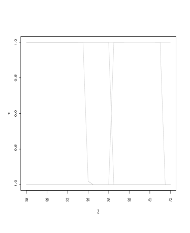
Figure 1: 500 realizations of $\eta_{i}(z)$ drawn from the prior distribution. The simulation setup is inspired by the real data example in Section 5: in the left panel $Z$ is uniform on (28,42) and in the right panel $Z$ has been standardized using the transformation $h(Z)=(Z-35)/7$.

Without additional information on the shape of $\eta_{i}$ we would like to be as vague as possible a priori. Note that the prior distributions given in equations (7) and (8) induce a prior distribution on the set of all possible maps $\eta_{i}:{\bf R}\rightarrow{\bf R}$. This prior is too complex to characterize analytically, but easy to sample from. Specifically, given a response index $i$, each sample of spline parameters $\{\zeta_{k}^{(i)},\gamma_{k}^{(i)},\psi_{k}^{(i)}:\;1\leq k\leq K_{\max}^{(i)}\}$, $\{\alpha_{j}^{(i)}:\;1\leq j\leq 3\}$ and $\alpha_{0}$ from (7) and (8) will produce, when plugged into equation (6), a curve $\eta_{i}$. If the priors used are indeed not too informative about the shape of $\eta_{i}$ then we do not expect to see emerging any particular patterns. Our numerical experiments show that the prior is not too sensitive to changes in the values used in (7) and (8), but is sensitive to the covariate’s range. In Figure 1 we show 500 maps $\eta_{i}(z)$ on the Kendall’s tau scale where it has bounded range $[-1,1]$. The left panel illustrates the case where the covariate is uniform on the interval $(28,42)$ (the range was chosen to match the data example in Section 3.5) and the curves in the right panel are obtained after standardizing the covariate so that the new range is $[-1,1]$. When the range for the covariate is large the prior weight is assigned mostly to extreme dependence patterns where Kendall’s tau is close to 1 or -1 for almost all values of $X$. Such priors are undesirable as they have the potential of biasing the inference. However, after standardizing the covariate, the prior bias seems to vanish. For this reason we recommend standardizing all covariates used in the conditional copula model.

2.1 The Computational Algorithm

If $\omega$ is the vector of all the parameters involved in the model and ${\cal D}$ are all the observed data, the posterior distribution $\pi(\omega|{\cal D})$ cannot be studied analytically due to its complicated form. Instead, we construct an Markov chain Monte Carlo (MCMC) algorithm to sample from $\pi(\omega|{\cal D})$. The form of the sampling algorithm follows the generic design of the Gibbs sampler (Gelfand, 2000) in which every component $\omega_{j}$ is updated by sampling from its conditional distribution $\pi(\omega_{j}|\omega\backslash\omega_{j},{\cal D})$. Some of the components of the chain cannot be sampled directly from the conditional distribution, so a Metropolis-Hastings update is needed (for details on using Metropolis-Hasting updates within the Gibbs sampler see, for instance, Craiu and Rosenthal, 2014). The strategies used to update each parameter at step $t+1$ are described below. The super index ^(t) indicates the iteration step.

$\beta$’s:

Let ${\bf X}\in{\bf R}^{n\times p}$ be the matrix whose rows are $X_{j}^{T}$, $1\leq j\leq n$ and ${\bf Y}_{1},{\bf Y}_{2}$ the response vectors, i.e. ${\bf Y}_{i}=\{Y_{ij}:\;1\leq j\leq n\}$. If we had not considered the copula factor to account for the dependence between the outcomes, the posterior conditional distribution of $\beta_{1},\beta_{2}$ would have been available in closed form

$$\tilde{\pi}_{i}(\beta_{i}|{\cal D},\sigma_{i}^{(t)})=\tilde{\pi}(\beta_{i}|{\bf X},{\bf Y}_{i},\sigma_{i}^{(t)})=n(\beta_{i};\mu_{i},\Sigma_{i}),\;i=1,2$$ (9)

where $n(x;a,b)$ is the density of a normal with mean vector $a$ and variance matrix $b$, and

$$\mu_{i} = ({\bf I}+{\bf X}^{T}{\bf X})^{-1}{\bf X}^{T}{\bf Y}_{i}$$ (10)

$$\Sigma_{i} = (\sigma_{i}^{(t)})^{2}({\bf I}+{\bf X}^{T}{\bf X}_{i})^{-1},\;\;i=1,2.$$

The update of each $\beta_{i}$ involves a mixture transition kernels. With probability $\lambda=0.8$ we update using an Independent Metropolis (IM) transition kernel in which the proposal distribution is $\tilde{\pi}_{i}(\beta_{i})$ and with probability $1-\lambda=0.2$ we update using a Random Walk Metropolis (RWM) with a Gaussian proposal with mean at the current value of $\beta_{i}$ and variance chosen so that the acceptance rate is between 20-30%.

$\sigma$’s:

Once again, without the copula component of the likelihood, the posterior conditional distribution of $\sigma_{i}$, given the data and $\beta_{1},\beta_{2}$, is available in closed form

$$\tilde{\pi}(\sigma_{i}|{\cal D},\beta_{i}^{(t+1)})=\tilde{\pi}(\sigma_{i}|{\bf X},{\bf Y}_{i},\beta_{i}^{(t+1)})=$$

$$= IG\left(0.1+{p+n\over 2},0.1+{(\beta_{i}^{(t+1)})^{T}\beta_{i}^{(t+1)}+({\bf Y}_{i}-{\bf X}\beta_{i}^{(t+1)})^{T}({\bf Y}_{i}-{\bf X}\beta_{i}^{(t+1)})\over 2}\right),\;i=1,2.$$

The updates are made according to an IM kernel in which the proposal density is $\tilde{\pi}(\sigma_{i}|{\bf X},{\bf Y}_{i},\beta_{i}^{(t+1)})$ for each $i=1,2$. The updating steps for $\beta$ and $\sigma$ lead to faster mixing compared to those defined in Craiu and Sabeti (2012) where only RWM updates were used, because the IM transition kernel allows the chain to jump around the target space and reduces autocorrelation.

$\alpha$’s:

Because there is no range restriction for each $\alpha_{k}^{(i)}$ and no direct sampling strategy is possible, we use the RWM-within-Gibbs with proposal variance tuned so that the acceptance rates are between 20-40%.

$\zeta$’s:

The updates are performed using the Metropolis-within-Gibbs strategy for the entire latent variable vector $\vec{\zeta}^{(i)}=(\zeta_{1}^{(i)},\ldots,\zeta_{K_{\max}}^{(i)})$. For updating $\vec{\zeta}^{(i)}$ we use two type of moves: we either add/delete a component (i.e. transforming a zero component into a one or vice-versa) or swap two components. We choose with probability half to either add/delete a component chosen or to permute two components of $\vec{\zeta}$ that are selected at random. Each proposed move is accepted or rejected based on a Metropolis-Hastings rule.

$\psi$’s:

If $\zeta_{k}^{(i)}=1$ we use the RWM-within-Gibbs strategy to update $\psi_{k}^{(i)}$ using proposals tuned so that the acceptance rates are between 20-50%. If $\zeta_{k}^{(i)}=0$, $\psi_{k}^{(i)}$ is updated using a random draw from its prior distribution that is automatically accepted.

$\gamma$’s:

If $\zeta_{k}^{(i)}=1$ we use an IM update for $\gamma_{k}^{(i)}$ using as proposal the prior distribution of $\gamma_{k}^{(i)}$. If $\zeta_{k}^{(i)}=0$ then the next state $\gamma_{k}^{(i)}$ is sampled from its prior and automatically accepted.

$\lambda$:

For $\lambda$ we use an IM update with proposal distribution equal to the prior, i.e. Bin$(0.5,K_{\max})$.

2.2 Cross Validated Marginal Likelihood Model Selection

The cross-validated, pseudo marginal likelihood (CVML) criterion of Geisser and Eddy (1979) is used to compare the predictive power of various models considered. Denote ${\cal M}$ such a generic model, characterized by regression parameters $\{\beta_{i},\sigma_{i}:\;i=1,2\}$ corresponding a subset of covariates, ${\bf X}$, and all the spline parameters involved in modelling the calibration function $\eta({\bf X})$. Denote the parameters in the model $\omega$, the data is ${\cal D}$ and for each $1\leq j\leq n$, ${\cal D}_{-j}$ denotes the remaining data after we have removed the covariates and responses pertaining to the $j$th item, $(Y_{1j},Y_{2j},X_{j})$. A selection criterion based on the CVML will choose the model ${\cal M}$ that maximizes the sum

$$CVML({\cal M})=\sum\limits_{j=1}^{n}\log p(Y_{1j},Y_{2j}|{\cal D}_{-j},{\cal M}).$$ (11)

One can see from (11) that the CVML criterion favours models that exhibit good average predictive power. The average is taken with respect to the parameters in the model so (11) is a function of the observed data only. From a Bayesian standpoint the computation of the criterion would be impractical if we were to proceed by performing separately $n$ data analyses, one for each sample of size $n-1$. However, the following simple derivation can be used to compute $CVML({\cal M})$ from a single Bayesian analysis of the whole data (see also Hanson et al., 2011). We have

$$E[p(Y_{1j},Y_{2j}|\omega)^{-1}] = {1\over p({\cal D}|{\cal M})}\int{p({\cal D}|\omega,{\cal M})p(\omega|{\cal M})\over p(Y_{1j},Y_{2j}|\omega,{\cal M})}d\omega={1\over p({\cal D}|{\cal M})}\int p({\cal D}_{{-j}}|\omega,{\cal M})p(\omega|{\cal M})d\omega=$$ (12)

$$= {p({\cal D}_{-j}|{\cal M})\over p({\cal D}|{\cal M})}={1\over p(Y_{1j},Y_{2j}|{\cal D}_{-j},{\cal M})},$$

where the first expectation is taken with respect to the posterior distribution of all parameters in the model, $\pi(\omega|{\cal D},{\cal M})=p({\cal D}|\omega,{\cal M})/p({\cal D}|{\cal M})$. Based on (12) we deduce that a Monte Carlo estimator of (11) is

$$\widehat{CVML}({\cal M})=\sum_{j=1}^{n}-\log\left[{1\over M}\sum\limits_{m=1}^{M}p(Y_{1j},Y_{2j}|\omega^{(m)},{\cal M})^{-1}\right],$$ (13)

where $\omega^{(1)},\omega^{(2)},\ldots,\omega^{(M)}$ are draws from the posterior distribution $\pi(\omega|{\cal D},{\cal M})$ obtained via the MCMC algorithm described in the previous section.

3 Simulations

The simulation study provides information about the average errors incurred when implementing the proposed estimation approach and illustrates the performance of the CVML criterion when it is used to select the copula family and the influential covariates in model (4).

3.1 Simulation Details

We have generated data using the Clayton copula using either a univariate or a bivariate calibration function. Marginally, the outcomes follow the distributions defined by the linear models specified in (3). All covariate values are independently sampled from the $\mbox{Uniform}[0,1]$ distribution. For the dependence structure we have considered two nonlinear calibration functions $\eta_{S1},\eta_{S2}$ defined as

$$\eta_{S1}(x)=\log[4.5-1.5\sin(\pi x)],$$

and

$$\eta_{S2}(x_{1},x_{2})=\log[4.5-\sin(x_{1})-\sin(x_{2})].$$

Under scenario S1 we simulate data using only one covariate so the true calibration function is $\eta_{S1}$ and under scenario S2 we generate data using the calibration $\eta_{S2}$. Marginally, under S1 and S2, each response variable is linked to, respectively, one or two covariates via a linear model with Gaussian errors, as specified in (3).

Each analysis has been independently replicated 50 times for samples of size $n=450$. We kept $K_{max}=4$ fixed throughout the simulation study. The MCMC sampler was run for 10,000 iterations and the first 3000 samples were discarded as burn-in. The simulation parameters used in the MCMC samplers were selected so that the acceptance probabilities are between 20-40%. The copula model data was generated using the copula library within R. The main steps of the MCMC sampler were implemented in C++ with the results processed in R.

3.2 Estimation of the Calibration Function

In this section we present plots and measures of the goodness-of-fit for the estimating procedure proposed in this. We focus on scenario S2 which is more challenging to fit.

To provide a graphical illustration of the fit, in Table 3 we show one-dimensional slices in the true surface (black line), the estimated surface (red line) and the two surfaces delimitating the pointwise 95% credible region (green lines). The slices are obtained when one of the two covariates is fixed at values in the set $\{-0.75,-0.25,0.25,0.75\}$. We observe that the credible bands grow wider near the boundaries of the covariate range and the bias gets also bigger when one of the covariate is closer to 1 or -1.

Table 5 contains the trace plots, the autocorrelation plots (up to lag 200) and the histograms of the posterior sample realizations for $\theta(-0.25,0.75)$, $\theta(0.75,-0.25)$ and ${\theta}(0.75,0.75)$. In general, the ACF plots and the trace plots look similar. In the histograms, the red line shows the true value of the calibration function. We observe that the samples for $\theta(0.75,0.75)$ are further from the true value when compared to the samples for $\theta(0.75,-0.25)$. This is consistent with our previous observation concerning the fit when covariate values are close to the boundary.

We also look at the model estimates for the normal regression parameters. Table 6 shows the trace plots, the autocorrelation plots and the histograms obtained from posterior samples corresponding to the linear regression model for the first outcome, $\beta_{11}$ and $\beta_{12}$, and the residual standard deviation $\sigma_{1}$. The parameters used in the second response regression yield similar plots.

The red line in the histograms represents the true value of the parameters. Although the ACF seems to be high for these estimates, the histograms suggest that the samples provide good estimates for the marginal models parameters.

For a more global summary, we approximate numerically the integrated variance (IVAR), squared bias (IBias²), and mean squared error (IMSE) using a grid of 400 equidistant points in the covariate space. The values are reported in Table 4. When comparing these measures across the two simulation scenarios, we notice a significant increase in the bias when the number of covariates is increased. This is not surprising since the sample size is kept constant, but we fit a significantly more complex model under scenario S2 than under S1.

3.3 Copula Selection

We explore the performance of the CVML criterion for choosing the correct copula family. Specifically, we fit the generated data using Clayton, Frank and Gumbel copula families. In Table 1 we report the percentage of correct decisions computed from 100 replicates. It can be noticed that there is a small decrease in accuracy for scenario S2 compared to S1 which is not surprising given that the former model is more complex than the latter.

3.4 Variable Selection

We have also examined the performance of CVML in selecting the covariates to be included in the model. We focused on data generated under scenario S2 and we fitted them using models with 1, 2, or 3 covariates. In all simulations results reported in this section we have used the correct Clayton copula to formulate the model.

If we denote ${\cal M}_{i}$ as the model with the first $i$ covariates included, then we see from the box plots shown in Table 2 that $CVML$ always selects ${\cal M}_{2}$ over ${\cal M}_{1}$ or ${\cal M}_{3}$. The difference in CVML values is larger between ${\cal M}_{2}$ and ${\cal M}_{1}$ than between ${\cal M}_{2}$ and ${\cal M}_{3}$, which is natural given the criterion’s connection to the models predictive power.

3.5 Application to the Twin Birth Data

The additive model approach is applied to a subset of the Matched Multiple Birth Data Set. The data containing all twin births in the United States from 1995 to 2000 enable detailed investigation of twin gestations. We consider the twin live births in which both babies survived their first year of life with mothers of age between 18 and 40. Of interest is the dependence between the birth weights of twins (in grams), denoted by BW1 and BW2, respectively. We consider a random sample of 450 twin live births and investigate the effect of two covariates, gestational age (GA) and maternal age (MA), on the dependence between BW1 and BW2.

We compare the model ${\cal M}_{1}$ in which the GA is the only covariate considered and model ${\cal M}_{2}$ in which GA and MA are the included covariates. We also compare three analyses based on three parametric copula families: Clayton, Frank and Gumbel. For each copula family we compute the CVML criterion for the models with both covariates (GA and MA) included. The results shown in the first row of Table 7 suggest that the Frank copula is more suitable for analyzing the data.

Under the Frank copula, model ${\cal M}_{1}$ is preferred with a CVML value of -5569.4 compared to -7683.7 obtained for ${\cal M}_{2}$. After deciding that ${\cal M}_{1}$ is preferred, we compare again the fit for ${\cal M}_{1}$ under each of the three copulas, and the results are shown on the second row of Table 7. This finding is concordant with the single covariate analysis of Acar et al. (2011).

4 Conclusions and Future Work

We propose Bayesian inference for the conditional copula model in a regression context with multiple covariates. We implement spline approximation within the additive model framework and propose a model selection criterion which selects the model with the best predictive power.

The simulations show that the efficiency of the method decreases as the dimension of the covariate vector increases and we would like to explore theoretically the rate of the decay. It is conceivable that when the number of covariates grows large, the approach proposed here may become too computationally expensive and simpler formulations of the calibration function and improvements of the MCMC algorithm needed to sample the posterior distribution are worth investigating.

Scenario $\backslash$ Copula	Frank	Gumbel
S1	100	98
S2	96	94

Table 1: PPerformance of CVML in selecting the correct Clayton family over Frank or Gumbel family under scenarios S1 and S2. The numbers in the table represent the percentage of correct decisions.

Table 2: Comparison of the CVML criterion values for models with 1,2, or 3 covariates. Left panel: box plot of 100 independently replicated values of the difference $CVML({\cal M}_{2})-CVML({\cal M}_{1})$. Right panel: box plot of 100 independently replicated values of the difference $CVML({\cal M}_{2})-CVML({\cal M}_{3})$.

Z1 is fixed	Z2 is fixed

Table 3: One-dimensional projections of the true calibration surface (black), the estimated surface (red) and confidence bands (green) produced under scenario S2.

Scenario	IBias2	IVAR	IMSE
S1	0.061	0.433	0.494
S2	0.132	0.515	0.647

Table 4: Performance of the estimation procedure under scenarios S1 and S2.

	$\hat{\theta}(-0.25,0.75)$	$\hat{\theta}(0.75,-0.25)$	$\hat{\theta}(0.75,0.75)$
Trace Plots
Acf Plots
Histogram

Table 5: Plot details for $\theta$ in the 10th run.

	$\beta_{11}$	$\beta_{12}$	$\sigma_{1}$
Trace Plots
Acf Plots
Histogram

Table 6: Trace (top row), ACF (middle row) and histogram (bottom row) plots for the regression coefficients of the first outcome, $\beta_{11}$ and $\beta_{12}$, and the corresponding residual standard deviation, $\sigma_{1}$.

Criterion	Clayton	Frank	Gumbel
$\mbox{CVML}({{\cal M}_{2}})$	-10213.4	-7683.7	-54763.2
$\mbox{CVML}({{\cal M}_{1}})$	-7405.3	-5569.4	-49947.9

Table 7: Twin Birth Data: CVML values for three copula families under model ${\cal M}_{1}$ (bottom row) and ${\cal M}_{2}$ (top row). The criterion suggests that the model ${\cal M}_{1}$ with the Frank copula is most suitable for fitting the data.

References

- Abegaz et al. (2012) Abegaz, F., Gijbels, I. and Veraverbeke, N. (2012). Semiparametric estimation of conditional copulas. J. Multivariate Anal., 110 43–73.
- Acar et al. (2011) Acar, E., Craiu, R. V. and Yao, F. (2011). Dependence calibration in conditional copulas: A nonparametric approach. Biometrics to appear.
- Acar et al. (2012) Acar, E., Genest, C. and Nešlehová, J. (2012). Beyond simplified pair-copula constructions. Journal of Multivariate Analysis, 110 74–90.
- Craiu and Rosenthal (2014) Craiu, R. V. and Rosenthal, J. S. (2014). Bayesian computation via Markov chain Monte Carlo. Annual Reviews of Statistics and Its Application to appear.
- Craiu and Sabeti (2012) Craiu, R. V. and Sabeti, A. (2012). In mixed company: Bayesian inference for bivariate conditional copula models with discrete and continuous outcomes. J. Multivariate Anal., 110 106–120.
- Geisser and Eddy (1979) Geisser, S. and Eddy, W. F. (1979). A predictive approach to model selection. J. Amer. Statist. Assoc., 74 153–160.
- Gelfand (2000) Gelfand, A. E. (2000). Gibbs sampling. J. Amer. Statist. Assoc., 95 1300–1304.
- Genest and Remillard (2004) Genest, C. and Remillard, B. (2004). Tests of independence and randomness based on the empirical copula process. Test, 13 335–369.
- Hanson et al. (2011) Hanson, T., Branscum, A. and Johnson, W. (2011). Predictive comparison of joint longitudinal-survival modeling: a case study illustrating competing approaches. Lifetime Data Analysis, 17 3–28.
- Hastie and Tibshirani (1990) Hastie, T. J. and Tibshirani, R. J. (1990). Generalized Additive Models. Chapman & Hall, London.
- Kojadinovic and Holmes (2009) Kojadinovic, I. and Holmes, M. (2009). Tests of independence among continuous random vectors based on cramér-von Mises functionals of the empirical copula process. J. Multivariate Anal., 100 1137–1154.
- Lambert and Vandenhende (2002) Lambert, P. and Vandenhende, F. (2002). A copula-based model for multivariate non-normal longitudinal data: analysis of a dose titration safety study on a new antidepressant. Statist. Medicine, 21 3197–3217.
- Omelka et al. (2009) Omelka, M., Gijbels, I. and Veraverbeke, N. (2009). Improved kernel estimation of copulas: Weak convergence and goodness-of-fit testing. Annals of Statistics, 37 3023–3058.
- Patton (2006) Patton, A. J. (2006). Modelling asymmetric exchange rate dependence. International Economic Review, 47 527–556.
- Sklar (1959) Sklar, A. (1959). Fonctions de répartition à dimensions et leurs marges. Publications de l’Institut de Statistique de l’Université de Paris, 8 229–231.
- Smith and Kohn (1996) Smith, M. and Kohn, R. (1996). Nonparametric regression using bayesian variable selection. Journal of Econometrics, 75 317–343.
- Székely et al. (2007) Székely, G. J., Rizzo, M. L. and Bakirov, N. K. (2007). Measuring and testing dependence by correlation of distances. Ann. Statist., 35 2769–2794.
- Veraverbeke et al. (2011) Veraverbeke, N., Omelka, M. and Gijbels, I. (2011). Estimation of a conditional copula and association measures. Scand. J. Statist. to appear.