Orbital–dependent second–order scaled–opposite–spin correlation functionals in the optimized effective potential method

Abstract

The performance of correlated optimized effective potential (OEP) functionals based on the spin–resolved second–order correlation energy is analyzed. The relative importance of singly– and doubly– excited contributions as well as the effect of scaling the same– and opposite– spin components is investigated in detail comparing OEP results with Kohn–Sham (KS) quantities determined via an inversion procedure using accurate ab initio electronic densities. Special attention is dedicated in particular to the recently proposed scaled–opposite–spin OEP functional [I. Grabowski, E. Fabiano and F. Della Sala, Phys. Rev. B, 87, 075103, (2013)] which is the most advantageous from a computational point of view. We find that for high accuracy a careful, system dependent, selection of the scaling coefficient is required. We analyze several size-extensive approaches for this selection. Finally, we find that a composite approach, named OEP2-SOSh, based on a post-SCF rescaling of the correlation energy can yield high accuracy for many properties, being comparable with the most accurate OEP procedures previously reported in the literature but at substantially reduced computational effort.

I Introduction

In recent years, ab initio correlation energy functionals for use in density-functional theory (DFT) have raised considerable interest, since they provide a systematic way to overcome the limitations of conventional (i.e. local or semi–local) density–dependent approximations dftbook3 , such as the presence of self–interaction error, qualitatively incorrect correlation potentials umrigar:1994:EXACT ; grabowski:2011:jcp , description of dispersion interactions furche11 ; galli11 and the Kohn–Sham (KS) occupied-virtual energy–gaps grun06 ; ls2 . The development of such functionals has followed different paths including the adiabatic–connection fluctuation–dissipation (ACFD) theorem lang75 ; lang77 , Görling–Levy Perturbation Theory (GLPT) gorling:1993:PT , many–body perturbation theory (MBPT) kutz09 ; grabowski:2002:OEPP2 ; ivanov:2003:P2 ; schweigert:2006:pt2 , and the idea of ab initio DFT bartlett:2005:abinit2 , in which the density condition gorling:1995:IJQCS together with coupled–cluster (CC) methodology is employed. In all cases the resulting correlation functionals depend explicitly on all the KS orbitals and eigenvalues (i.e. both occupied and virtual). Thus, for a full self–consistent–field (SCF) solution of the KS equations, the optimized effective potential (OEP) method goe05 ; kummelrmp08 ; lhf2 ; engel11book must be employed.

The OEP method is nowadays widely established for exact exchange (EXX or OEPx) in calculations on both molecular gorling:1999:OEP ; ivanov:1999:OEP ; yang:2002:OEP ; hesselmanexx07 ; heatonburgess07 ; filatov10 and solid–state systems Stadele97 ; grun06 ; sharma07 ; blugel11 . Hence, the OEPx method and its approximations lhf1 ; lhf2 ; ceda ; elp ; staroverov2 are gaining popularity, especially because they remove the one–electron self–interaction error (SIE) and strongly improve the KS eigenvalue spectrum as compared to conventional density–dependent functionals goe05 ; kummelrmp08 ; lhf2 ; engel11book .

In contrast, correlated OEP calculations are much less common in the literature and they are still an open research topic for development and testing. In particular, correlated calculations based on the ACFD approach, starting from the Random–Phase–Approximation (RPA) level, are usually only performed in a post–SCF fashion, i.e. using orbitals and eigenvalues from conventional KS calculations employing a semilocal functional furche08 ; kresse09 ; xen11 ; hess11 ; furche12 ; hutter13 or the OEPx goe11 ; goe10 ; hess11 method. In fact, a stable and efficient full–SCF OEP–RPA solution is difficult to achieve hellgren07 ; hellgren12 ; verma:044105 and only very recently an approach for large systems has been presented goe13 . Moreover, the direct RPA i) shows large inaccuracies for thermochemistry, so that different extensions have been presented in recent years paier10 ; xen11 ; furche13 ; sosex ; ren13 , but all lacking a corresponding correlation potential; ii) has a computational cost about one order of magnitude larger than the one for the second–order correlation hutter13 ; iii) requires larger basis sets than second–order correlation kresse12 ; furche12basis ; fabiano12 .

More successful implementations of full SCF correlated OEP calculations have been obtained in the context of perturbation theory, in most cases restricted to the use of second–order correlation. Thus, as a common practice correlated OEP calculations are based on the second–order GLPT (OEP–GL2), since this leads to a reliable and physically sound, although overestimated bonetti01 ; grabowski:2002:OEPP2 ; bartlett:2005:abinit2 ; mori-sanchez:2005:oeppt2 ; schweigert:2006:pt2 , description of correlation effects. Nevertheless, because GLPT2 is unbounded from below, a variational collapse is possible for unphysical exchange–correlation potentials rohr-baerends:2006:oephe ; engel:2005:oeppt2 . These potentials do not correspond to KS solutions and can be in general easily excluded by minimal regularization (such as the truncated SVD approach used in the present work). Nonetheless for special cases numerical instabilities can persist.

To improve stability and accuracy new approaches have been proposed. One of these is based on a modified MBPT(2) functional with a semi–canonical transformation of the Hamiltonian (OEP2–sc) bartlett:2005:abinit2 ; schweigert:2006:pt2 ; grabowski:2007:ccpt2 . As an alternative, recently a new method (OEP2–SOS) sos_oep2:prb has been proposed in this context, based on the spin–resolved second–order correlation energy expression grimme03 , and especially on the scaled–opposite–spin (SOS) variant thereof. This method takes advantage of the improved accuracy demonstrated for spin–component–scaled (SCS) and SOS second–order Møller–Plesset (MP2) calculations WCMS12 ; grimme03 and provides an accurate OEP correlation functional that largely outperforms the OEP–GL2 approach sos_oep2:prb . Moreover, the OEP2–SOS method demonstrated a clear advantage over the OEP–GL2 method, converging also in difficult cases (e.g., the Beryllium atom). In fact the OEP2-SOS method employs a scaled (smaller) correlation potential as compared to OEP-GL2, and thus the former yields larger energy-gaps and it is less prone to variational collapse than the lattersos_oep2:prb . Finally, because only the opposite–spin correlation is involved in its formulation, the OEP2–SOS functional has a favourable computational cost with respect to other second–order approaches ($\mathcal{O}(N^{4})$ vs. $\mathcal{O}(N^{5})$).

The OEP2–SOS method is thus a promising approach for ab initio correlated DFT calculations. Nevertheless, a systematic and detailed test of its performance is still lacking, since in Ref. 58 only a few systems were considered in the test set. Moreover, no investigation was performed to inspect the role of the different components of the spin–resolved second–order correlation (namely the opposite–spin (OS), same–spin (SS), and singly excited (SE) contributions) and determine optimal scaling coefficients for different properties. In this paper we conduct a thorough investigation of the SCS and SOS second–order OEP correlation, by analysing the specific contribution of the different components of the spin–resolved second–order OEP correlation and the overall performance of several variants of the method. To perform this analysis we compare the correlation energies obtained with accurate coupled-cluster singles-doubles with perturbative triples [CCSD(T)] values. In addition, we compare the resulting KS orbital energies and electronic densities with accurate KS values determined using an inversion procedure based on the CCSD(T) electronic densities.

II Theory

For a given orbital– and eigenvalue–dependent exchange–correlation (XC) energy functional ($E_{\mathrm{xc}}$) the OEP equation for the XC potential reads sharp:1953:OEP ; talman:1976:OEP ; krieger:1990:OEP ; gorling:1995:IJQCS ; grabowski:2002:OEPP2 ; kummel:2008:oep ; lhf2 ; engel:2003:3GDFT

$$\int X_{\sigma}(\mathbf{r},\mathbf{r}^{\prime})v_{\mathrm{xc},\sigma}^{\mathrm{OEP}}({\mathbf{r}^{\prime}})\mathrm{d}\mathbf{r}^{\prime}=\Lambda_{\mathrm{xc},\sigma}(\mathbf{r})\,,$$ (1)

which is an integral equation (Fredholm of the first kind) with the inhomogeneity given by

$$\Lambda_{\mathrm{xc},\sigma}(\mathbf{r}) = \sum_{p}\bigg{\{}\int\phi_{p\sigma}(\mathbf{r})\sum_{q\neq p}\frac{\phi_{q\sigma}(\mathbf{r})\phi_{q\sigma}(\mathbf{r}^{\prime})}{\epsilon_{p\sigma}-\epsilon_{q\sigma}}\frac{\delta E_{\mathrm{xc}}}{\delta\phi_{p\sigma}(\mathbf{r}^{\prime})}\mathrm{d}\mathbf{r}^{\prime}$$ (2)

$$+\frac{\delta E_{\mathrm{xc}}}{\delta\epsilon_{p\sigma}}|\phi_{p\sigma}(\mathbf{r})|^{2}\bigg{\}}$$

where the index $\sigma$ labels the spin (throughout this work we denote the spin indicies $\sigma,\tau\ldots$), $X_{\sigma}^{-1}$ is the inverse of the static KS linear response function

$$X_{\sigma}(\mathbf{r}^{\prime},\mathbf{r})=2\sum_{ia}\frac{\phi_{i\sigma}(\mathbf{r}^{\prime})\phi_{a\sigma}(\mathbf{r}^{\prime})\phi_{a\sigma}(\mathbf{r})\phi_{i\sigma}(\mathbf{r})}{\epsilon_{i\sigma}-\epsilon_{a\sigma}}\ ,$$ (3)

and $\phi_{p\sigma}$ and $\epsilon_{p\sigma}$ denote the KS orbitals and eigenvalues, respectively, determined by the KS equations

$$\left[-\frac{1}{2}\nabla^{2}+v_{\mathrm{ext}}({\bf r})+v_{\mathrm{J}}({\bf r})+v_{\mathrm{xc},\sigma}^{\mathrm{OEP}}({\bf r})\right]\phi_{p\sigma}({\bf r})=\epsilon_{p\sigma}\phi_{p\sigma}({\bf r})\ ,$$ (4)

with $v_{\mathrm{ext}}({\bf r})$ and $v_{\mathrm{J}}({\bf r})$ the external (nuclear) and the Coulomb potentials, respectively. In all equations we use the convention that $i,j,k$ label occupied KS orbitals, $a,b,c$ label virtual ones, while the indexes $p,q,r,s$ are used otherwise.

It is useful in orbital dependent approaches to divide the XC energy as $E_{\mathrm{xc}}=E_{\mathrm{x}}+E_{\mathrm{c}}$, separating the exchange and the correlation contributions. The exchange energy functional has the form of the usual Hartree–Fock exchange energy

$$E_{\mathrm{x}}[\{\phi_{q\tau}\}]=-\frac{1}{2}\sum_{\sigma}\sum_{ij}(i_{\sigma}j_{\sigma}|j_{\sigma}i_{\sigma})\ ,$$ (5)

with $(p_{\sigma}q_{\sigma}|r_{\sigma}s_{\sigma})$ being a two–electron integral in the Mulliken notation computed from KS orbitals. The corresponding OEP KS exact–exchange potential is labeled OEPx and defined by the equation

$$v_{\mathrm{x},\sigma}^{\mathrm{OEPx}}(\mathbf{r}) =-2\sum_{ij}\sum_{a}\int\frac{(i_{\sigma}j_{\sigma}|j_{\sigma}a_{\sigma})}{\epsilon_{i\sigma}-\epsilon_{a\sigma}}$$ (6)

$$\times\phi_{a\sigma}(\mathbf{r}^{\prime})\phi_{i\sigma}(\mathbf{r}^{\prime})X^{-1}_{\sigma}(\mathbf{r}^{\prime},\mathbf{r})d\mathbf{r}^{\prime}\ .$$

For the correlation part, we consider the spin–resolved expression obtained from the second–order Görling–Levy perturbation theory (GLPT) energy functional gorling:1993:PT , which has exactly the same form as a functional defined from the many–body perturbation theory (MBPT) grabowski:2002:OEPP2 ; ivanov:2003:P2

$$E_{c}^{(2)}=c_{\mathrm{OS}}E_{\mathrm{OS}}+c_{\mathrm{SS}}E_{\mathrm{SS}}+E_{\mathrm{SE}}\ ,$$ (7)

where

$$E_{\mathrm{OS}} = \frac{1}{2}\sum_{\sigma}\sum_{\tau\neq\sigma}\sum_{ij}\sum_{ab}\frac{\left|(i_{\sigma}a_{\sigma}|j_{\tau}b_{\tau})\right|^{2}}{\epsilon_{i\sigma}+\epsilon_{j\tau}-\epsilon_{a\sigma}-\epsilon_{b\tau}}$$ (8)

$$E_{\mathrm{SS}} = \frac{1}{2}\sum_{\sigma}\sum_{ij}\sum_{ab}\frac{\left|(i_{\sigma}a_{\sigma}|j_{\sigma}b_{\sigma})\right|^{2}}{\epsilon_{i\sigma}+\epsilon_{j\sigma}-\epsilon_{a\sigma}-\epsilon_{b\sigma}}$$ (9)

$$-\frac{1}{2}\sum_{\sigma}\sum_{ij}\sum_{ab}\frac{(i_{\sigma}a_{\sigma}|j_{\sigma}b_{\sigma})(a_{\sigma}j_{\sigma}|b_{\sigma}i_{\sigma})}{\epsilon_{i\sigma}+\epsilon_{j\sigma}-\epsilon_{a\sigma}-\epsilon_{b\sigma}}$$

$$E_{\mathrm{SE}} = \sum_{\sigma}\sum_{ia}\frac{|f^{\sigma}_{ia}|^{2}}{\epsilon_{i\sigma}-\epsilon_{a\sigma}},$$ (10)

while $c_{\mathrm{OS}}$ and $c_{\mathrm{SS}}$ are simple scaling factors for the opposite–spin (OS) and same–spin (SS) correlation, respectively. Note that the correlation functional of Eq. (7) includes also a singly excited term, depending on the square of the Fock matrix elements

$$f^{\sigma}_{pq}=\varepsilon_{p_{\sigma}}^{\mathrm{KS}}\delta_{p_{\sigma}q_{\sigma}}-\langle p_{\sigma}|\hat{K}_{\sigma}+v_{\mathrm{x},\sigma}^{OEP}|q_{\sigma}\rangle,$$ (11)

with $\hat{K}$ the nonlocal Hartree–Fock exchange operator. This term arises because in the present case the correlation energy through second–order is computed using KS orbitals instead of canonical Hartree–Fock ones. The OEP correlation potential corresponding to the functional of Eq. (7) is obtained from Eq. (1) as

$$v_{\mathrm{c},\sigma}^{\mathrm{OEP}}(\mathbf{r})=c_{\mathrm{OS}}v_{\mathrm{OS},\sigma}(\mathbf{r})+c_{\mathrm{SS}}v_{\mathrm{SS},\sigma}(\mathbf{r})+v_{\mathrm{SE},\sigma}(\mathbf{r})\ ,$$ (12)

with

$$v_{\mathrm{OS},\sigma}(\mathbf{r}) = \sum_{\tau\neq\sigma}\sum_{ij}\sum_{ab}\int\Bigg{\{}\frac{(i_{\tau}a_{\tau}|j_{\sigma}b_{\sigma})}{\epsilon_{i\tau}+\epsilon_{j\sigma}-\epsilon_{a\tau}-\epsilon_{b\sigma}}$$ (13)

$$\times\bigg{[}2\sum_{p\neq j}\frac{(i_{\tau}a_{\tau}|p_{\sigma}b_{\sigma})}{\epsilon_{j\sigma}-\epsilon_{p\sigma}}\phi_{j\sigma}(\mathbf{r}^{\prime})\phi_{p\sigma}(\mathbf{r}^{\prime})$$

$$+2\sum_{p\neq b}\frac{(i_{\tau}a_{\tau}|j_{\sigma}p_{\sigma})}{\epsilon_{b\sigma}-\epsilon_{p\sigma}}\phi_{p\sigma}(\mathbf{r}^{\prime})\phi_{b\sigma}(\mathbf{r}^{\prime})$$

$$-\frac{(i_{\tau}a_{\tau}|j_{\sigma}b_{\sigma})}{\epsilon_{i\tau}+\epsilon_{j\sigma}-\epsilon_{a\tau}-\epsilon_{b\sigma}}\Big{(}\phi_{j\sigma}(\mathbf{r}^{\prime})\phi_{j\sigma}(\mathbf{r}^{\prime})$$

$$-\phi_{b\sigma}(\mathbf{r}^{\prime})\phi_{b\sigma}(\mathbf{r}^{\prime})\Big{)}\bigg{]}\Bigg{\}}X_{\sigma}^{-1}(\mathbf{r}^{\prime},\mathbf{r})d\mathbf{r}^{\prime}$$

$$v_{\mathrm{SS},\sigma}(\mathbf{r}) = \sum_{ij}\sum_{ab}\int\Bigg{\{}\frac{(i_{\sigma}a_{\sigma}|j_{\sigma}b_{\sigma})-(a_{\sigma}j_{\sigma}|b_{\sigma}i_{\sigma})}{\epsilon_{i\sigma}+\epsilon_{j\sigma}-\epsilon_{a\sigma}-\epsilon_{b\sigma}}$$ (14)

$$\times\bigg{[}2\sum_{p\neq i}\frac{(p_{\sigma}a_{\sigma}|j_{\sigma}b_{\sigma})}{\epsilon_{i\sigma}-\epsilon_{p\sigma}}\phi_{i\sigma}(\mathbf{r}^{\prime})\phi_{p\sigma}(\mathbf{r}^{\prime})$$

$$+2\sum_{p\neq a}\frac{(i_{\sigma}p_{\sigma}|j_{\sigma}b_{\sigma})}{\epsilon_{a\sigma}-\epsilon_{p\sigma}}\phi_{p\sigma}(\mathbf{r}^{\prime})\phi_{a\sigma}(\mathbf{r}^{\prime})$$

$$-\frac{1}{2}\frac{(i_{\sigma}a_{\sigma}|j_{\sigma}b_{\sigma})}{\epsilon_{i\sigma}+\epsilon_{j\sigma}-\epsilon_{a\sigma}-\epsilon_{b\sigma}}\Big{(}\phi_{i\sigma}(\mathbf{r}^{\prime})\phi_{i\sigma}(\mathbf{r}^{\prime})$$

$$+\phi_{j\sigma}(\mathbf{r}^{\prime})\phi_{j\sigma}(\mathbf{r}^{\prime})-\phi_{a\sigma}(\mathbf{r}^{\prime})\phi_{a\sigma}(\mathbf{r}^{\prime})$$

$$-\phi_{b\sigma}(\mathbf{r}^{\prime})\phi_{b\sigma}(\mathbf{r}^{\prime})\Big{)}\bigg{]}\Bigg{\}}X_{\sigma}^{-1}(\mathbf{r}^{\prime},\mathbf{r})d\mathbf{r}^{\prime}$$

$$v_{\mathrm{SE},\sigma}(\mathbf{r}) = 2\sum_{ia}\int\Bigg{\{}\frac{f^{\sigma}_{ia}}{\epsilon_{i\sigma}-\epsilon_{a\sigma}}\bigg{[}\sum_{p\neq i}\frac{\phi_{p\sigma}(\mathbf{r}^{\prime})\phi_{i\sigma}(\mathbf{r}^{\prime})}{\epsilon_{i\sigma}-\epsilon_{p\sigma}}f^{\sigma}_{pa}$$ (15)

$$+\sum_{p\neq a}\frac{\phi_{p\sigma}(\mathbf{r}^{\prime})\phi_{a\sigma}(\mathbf{r}^{\prime})}{\epsilon_{a\sigma}-\epsilon_{p\sigma}}f^{\sigma}_{ip}+\sum_{kc}\frac{\phi_{c\sigma}(\mathbf{r}^{\prime})\phi_{k\sigma}(\mathbf{r}^{\prime})}{\epsilon_{k\sigma}-\epsilon_{c\sigma}}$$

$$\times\Big{(}2(i_{\sigma}a_{\sigma}|c_{\sigma}k_{\sigma})-(i_{\sigma}c_{\sigma}|k_{\sigma}a_{\sigma})-(i_{\sigma}k_{\sigma}|c_{\sigma}a_{\sigma})\Big{)}$$

$$-\frac{1}{2}\frac{f^{\sigma}_{ia}}{\epsilon_{i\sigma}-\epsilon_{a\sigma}}\Big{(}\phi_{i\sigma}(\mathbf{r}^{\prime})\phi_{i\sigma}(\mathbf{r}^{\prime})-\phi_{a\sigma}(\mathbf{r}^{\prime})\phi_{a\sigma}(\mathbf{r}^{\prime})\Big{)}\bigg{]}\Bigg{\}}$$

$$\times X^{-1}_{\sigma}(\mathbf{r}^{\prime},\mathbf{r})d\mathbf{r}^{\prime}\ .$$

III Computational methodology

Equations (6) and (12)-(15) provide formal expressions for the exchange and correlation potentials, respectively. However, to calculate the OEP exchange and correlation potentials in practice we employ the finite–basis set procedure of Refs. 21; 22; 66. Thus, the OEP is expanded as

$$v_{\mathrm{xc},\sigma}^{\mathrm{OEP}}(\mathbf{r})=v_{\mathrm{Slater}}^{\sigma}(\mathbf{r})+\sum_{l=1}^{N_{\mathrm{aux}}}c_{l}^{\sigma}g_{l}(\mathbf{r})\ ,$$ (16)

and this ansatz is used to solve the OEP equation (Eq. (1)). The first term on the right hand side is the Slater potential

$$v_{\mathrm{Slater}}^{\sigma}(\mathbf{r})=-\sum_{ij}\frac{\phi_{i\sigma}(\mathbf{r})\phi_{j\sigma}(\mathbf{r})}{\rho_{\sigma}(\mathbf{r})}\int\frac{\phi_{i\sigma}(\mathbf{r}^{\prime})\phi_{j\sigma}(\mathbf{r}^{\prime})}{|\mathbf{r}-\mathbf{r}^{\prime}|}d\mathbf{r}^{\prime}$$ (17)

which is added to ensure the correct $-1/r$ asymptotic behaviour of the potential. The second term is an expansion in $N_{\mathrm{aux}}$ Gaussian basis functions $g_{l}(\mathbf{r})$ with the expansion coefficients $c_{l}^{\sigma}$ determined from the solution of the OEP equations with the total $v_{\mathrm{xc},\sigma}^{\mathrm{OEP}}=v_{\mathrm{x},\sigma}^{\mathrm{OEP}}+v_{\mathrm{c},\sigma}^{\mathrm{OEP}}$ potentials defined by Eq. (6) and Eqs. (12)-(15) for exchange and correlation potentials respectively.

Note that Eq. (16) cannot correctly describe the exact OEP potential in the asymptotic region for molecules with HOMO nodal surfaces (HNSs), i.e. H₂O, NH₃, C₂H₆ in our test set. In fact, for these molecules the exact OEP potential is characterized by asymptotic barrier-well structures near HNSs lhfasy ; prlasy which cannot be represented in a (finite) linear combination of Gaussian functions. As shown in Refs. 67; 68, the asymptotic barrier-well structures will significantly influence high-lying virtual orbitals (LUMO+1 and above) so that the total correlation energies and correlation potentials can be expected to be influenced as well. We computed the GL2 correlation energy for C₂H₆ using localized Hartrre-Fock (LHF) lhf1 orbitals with and without the correct treatment of the asymptotic region lhfasy ; prlasy and we found a very small difference (about 1 mH). However, the description of the asymptotic region of correlated OEP method is beyond the target on this work.

Numerical instabilities in the solution of the OEP equations hirata:2001:OEPU ; elp ; hesselmanexx07 ; Joubert1 ; Kollmar1 ; Teale1 ; Glushkov1 ; Theophilou1 ; grabowski:2005:1shot ; grabowski:2007:ccpt2 ; bulat:2007:sn were minimized by a careful choice of the basis set (see Sec. III.1 for further details). Our calculations employ a truncated singular-value decomposition (SVD) for the construction of the pseudo-inverse of the linear response function in the OEP procedure. This regularization is an essential step in determining stable solutions to Eq. (1) and, together with the choice of basis set, ensures that stable and physically sound solutions are obtained.

In the present work we consider a full family of spin–component–scaled (SCS) second-order OEP (OEP2) methods, obtained using the correlation energy contributions in Eqs. (7)–(10) and the corresponding correlation potentials of Eqs. (12)–(15) with different values of the parameters $c_{\mathrm{OS}}$ and $c_{\mathrm{SS}}$ . These methods are denoted in general as OEP2–SCS. Moreover, special attention is devoted to OEP approaches based only on the opposite–spin part of the correlation, which are generally labeled as OEP2–SOS and described in more detail in Sections IV.3 and IV.4. Finally, we consider, for comparison also the OEP–GL2 grabowski:2002:OEPP2 ; engel:2005:oeppt2 ; mori-sanchez:2005:oeppt2 and OEP2–sc bartlett:2005:abinit2 methods. We note that the former is also a member of the family of the OEP2–SCS methods, being obtained by setting $c_{\mathrm{SS}}=c_{\mathrm{OS}}=1$.

Finally, we point out that, unfortunately, our current pilot OEP2-SOS implementation in ACESII acesii does not have the $\mathcal{O}(N^{4})$ scaling yet enabled. This does not significantly impact the efficiency of the calculations presented here for relatively small systems, however, it is an important advantage for larger systems and basis sets.

III.1 Computational details

To test the various OEP2–SCS approaches we performed calculations on several atomic (He, Be, Ne, Mg, Ar) and molecular (H₂, He₂, HF, CO, H₂O, Cl₂, N₂, Ne₂ HCl, NH₃, C₂H₆) systems using the the ACES II package acesii . For all systems we considered equilibrium geometries from Refs. 78; 79; 80. The geometries are as follows: H₂ H–H = 0.7461Å; He₂ He–He = 5.6Å; N₂ N–N = 1.098Å; Ne₂ Ne–Ne = 3.1Å; HF H–F = 0.9169Å; HCl H–Cl = 1.2746Å; Cl₂ Cl–Cl = 1.9871Å; CO C–O = 1.128Å; H₂O H–O = 0.959Å, H–O–H = 103.9^∘ ; NH₃ N–H = 1.008Å, H–N–H = 111.552^∘ ; C₂H₆ C–C = 1.533Å, C–H = 1.107Å, H–C–C = 109.3^∘ , H-C-H = 109.642^∘ .

In the present work we use the same basis set for the representation of both the orbitals and the OEP potential (i.e. the principal and the auxiliary basis sets are the same). Whilst this combination may not be optimal in terms of the balance between the potential and orbital descriptions hesselmanexx07 it has been shown to give reasonable results and a rationale for this has been presented by Filatov et al. in Ref. 26. To ensure that the basis sets chosen were flexible enough for both representation of the orbitals and potentials, all basis sets were constructed by full uncontraction of medium size (triple zeta) basis sets originally developed for correlated calculations as in Refs. 3; 81. In particular, we employed an even tempered $20s10p2d$ basis for He atom and He₂ molecule, an uncontracted ROOS–ATZP basis widm90 for Be, Ne atom and Ne₂ molecule, and an uncontracted aug–cc–pVTZ basis set woon93 for Mg atom. For the Ar atom we used a modified basis set which combines $s$ and $p$ type basis functions from the uncontracted ROOS–ATZP widm90 with $d$ and $f$ functions coming from the uncontracted aug–cc–pwCVQZ basis set peterson02 . The uncontracted cc–pVTZ basis set of Dunning dunning:1989:bas was used for all other systems.

For all OEP–KS calculations tight convergence criteria were enforced, e.g. for the SCF, corresponding to maximum deviations in density matrix elements of 10^-8 au. In addition the truncated SVD cutoff was set to 10^-6 and results were carefully checked to ensure convergence with respect to this parameter. As a further test of the stability of our results we computed the gradient of the total electronic energy with respect to variations of the $c_{l}^{\sigma}$ coefficients in Eq. (16): in all cases the computed gradient had a norm less than 10^-12 and the energies computed at the perturbed coefficients were higher than those obtained in our converged calculations, consistent with an energy minima.

To assess the OEP results we considered reference data from the OEP2–sc method bartlett:2005:abinit2 and benchmark data from second–order Møller–Plesset perturbation theory (MP2) moll34 , scaled–opposite–spin (SOS) MP2 jung04 , and coupled cluster singles–doubles with perturbative triples [CCSD(T)] :/content/aip/journal/jcp/76/4/10.1063/1.443164 ; :/content/aip/journal/jcp/89/12/10.1063/1.455269 ; :/content/aip/journal/jcp/87/10/10.1063/1.453520 ; Raghavachari1989479 calculations. In the MP2 and CCSD(T) cases relaxed densities were obtained from relaxed density matrices hansch:1984:zvec ; ricamo:1985:relden ; bartlett:1986:relden ; bartlett:1989:relden constructed using the Lagrangian approach helg:1989:lag ; jorg:1988:lag ; koch:1990:lag ; hald:2003:lag , while KS potentials and the corresponding single–particle orbitals were constructed by employing the inversion approach of Wu and Yang wu:2003:wy . In these calculations the smoothing–norm approach of Refs. 101; 76 was employed with a regularization parameter of $10^{-5}$. The calculations were considered converged when the gradient norm was below $10^{-6}$. The results of this inversion approach when applied to MP2 and CCSD(T) relaxed densities were denoted by KS[MP2] and KS[CCSD(T)] respectively. All benchmark calculations were carried out with a development version of the Dalton2013 quantum chemistry program DALTON ; DALPAP .

To assess the performance of each approach we considered the following quantities relative to CCSD(T) and KS[CCSD(T)].

i) Absolute differences in the correlation energy

$$\Delta E_{\mathrm{c}} = \left|E_{\mathrm{c}}^{\mathrm{method}}-E_{\mathrm{c}}^{\mathrm{CCSD(T)}}\right|$$ (18)

Note that we compared DFT correlation energies with WFT ones; see discussion in Section IV.4.

ii) Absolute differences in the energy gap between the lowest unoccupied molecular orbital (LUMO) and the highest occupied molecular orbital (HOMO)

$$\Delta\mathrm{HL} = \Big{|}\epsilon_{\mathrm{L}}^{\mathrm{method}}-\epsilon_{\mathrm{H}}^{\mathrm{method}}$$

$$-\left(\epsilon_{\mathrm{L}}^{\mathrm{KS[CCSD(T)]}}-\epsilon_{\mathrm{H}}^{\mathrm{KS[CCSD(T)]}}\right)\Big{|}\ .$$

We remark that this quantity is an important indicator because it is not only directly related to the quality of the OEP potential, which determines the orbital energies, but also because within time-dependent DFT the HOMO-LUMO gap is the zero-th order approximation for excitation energies. We also note that all of our calculations deliver LUMO orbitals that are bound, this is consistent with the fact that the KS equations (in contrast to the Hartree–Fock ones) contain the same local self-interaction free potential for all orbitals (both occupied and virtual).

iii) The integrated density differences (IDD)

$$\mathrm{IDD} = \int_{r_{0}}^{+\infty}\Omega(r)\left|\rho^{\mathrm{method}}(r)-\rho^{\mathrm{CCSD(T)}}(r)\right|dr$$ (20)

where $\Omega(r)=4\pi r^{2}$ and $r_{0}=0$ for atoms, while for linear molecules $\Omega(r)=1$, $r_{0}=-\infty$ and $r$ is the distance along the main axis . We note that the IDD is directly related in atoms and molecules with the difference radial density distribution Jankowski:2009:DRD $\mathrm{DRD}(r)=4\pi r^{2}(\rho^{\mathrm{method}}(r)-\rho^{\mathrm{xref}}(r))$ and the difference total density distribution (correlated density) $\rho_{c}(r)=(\rho^{\mathrm{method}}(r)-\rho^{\mathrm{xref}}(r))$, respectively, where xref=OEPx for correlated OEP methods and xref=Hartree–Fock for conventional wave function correlated methods. Thus, it provides also a direct test of the quality of the correlation potential.

IV Results

In this section we present the results of various OEP2-SCS calculations and compare them with benchmark values. In particular, we analyse the importance of the singly excited term for both the energies and the potentials and the role of the different values of the scaling parameters $c_{\mathrm{OS}}$ and $c_{\mathrm{SS}}$.

IV.1 Role of the singly excited term

To inspect the role of the singly excited term in the second–order correlation energy we report in Table 1 the decomposition of the energy according to Eq. (7) for several systems.

Table 1: Total correlation energy (m$E_{\mathrm{h}}$) and its components according to Eq. (7) for OEP–GL2 calculations on several atoms and molecules. In the last line we report the percentage contribution of each term to the total correlation energy.

System	$E_{c}^{\mathrm{OEP-GL2}}$	$E_{\mathrm{SS}}^{\mathrm{OEP-GL2}}$	$E_{\mathrm{OS}}^{\mathrm{OEP-GL2}}$	$E_{\mathrm{SE}}^{\mathrm{OEP-GL2}}$
He	-46.24	0.00	-46.24	0.00
Ne	-457.82	-113.43	-342.77	-1.61
Ar	-776.35	-205.02	-565.86	-5.46
Mg	-277.20	-54.56	-219.35	-3.28
H2	-48.55	0.00	-48.55	0.00
He2	-92.47	0.00	-92.47	0.00
HF	-464.76	-113.35	-349.13	-2.28
CO	-863.12	-210.34	-646.91	-5.87
H2O	-466.33	-108.76	-354.95	-2.63
HCl	-516.48	-125.58	-385.10	-5.80
Cl2	-1025.12	-255.99	-753.73	-15.40
N2	-866.33	-210.47	-649.93	-5.93
Ne2	-915.95	-226.99	-685.71	-3.26
NH3	-421.59	-90.13	-329.01	-2.45
C2H6	-693.66	-134.40	-552.81	-6.44
%		18.8%	80.6%	0.6%

Inspection of the table shows that the contribution of the singly excited term is indeed very small, amounting to a few m$E_{\mathrm{h}}$ in most systems, with the notable exception of Cl₂ where $E_{\mathrm{SE}}^{\mathrm{OEP-GL2}}$=$-$15.40 m$E_{\mathrm{h}}$ ( anyway this is only 1.5% of the total $E_{c}^{\mathrm{OEP-GL2}}$ energy). Thus, the singly excited term contributes only slightly to the total OEP correlation energy, giving on average a contribution lower than 1%. More importantly, this contribution is much smaller than the typical error of the OEP–GL2 method with respect to accurate benchmark correlation energies (e.g. CCSD(T)). For most systems, in fact, the errors relative to CCSD(T) are found to be on the order of several tens of m$E_{\mathrm{h}}$ (see Table 2) and for Cl₂ the error in the $E_{c}^{\mathrm{OEP-GL2}}$ energy is more than 150 m$E_{\mathrm{h}}$.

An even less important role is played by the singly excited term when the correlation potential is considered. This is shown in Figure 1 where we report the plot of the correlation KS potential and the DRD for the Neon atom, as a typical case. Similar results are obtained for other systems. The figure shows that, on the scale of the plots, the contribution of the singly excited term to the correlation potential is almost negligible Thus, almost no effect can be expected from the singly excited term on density–related and single–particle properties (e.g. multipole moments or orbital energies).

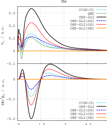
Figure 1: Correlation potentials (top) and DRD (=$4\pi\rho_{\mathrm{c}}$) (bottom) for the Ne atom as resulting from different components of the $v_{\mathrm{c}}^{\mathrm{OEP-GL2}}$ potential.

This result apparently contrasts the usual finding for the calculation of MP2 relaxed densities, where the single excitations display a non-negligible role (note that such contributions are included in all MP2 density calculations in this work). This difference can be rationalized considering that in the case of MP2 (based on fixed Hartree–Fock orbitals) the single excitations must account for significant orbital relaxation effects. In contrast, in the present OEP2- calculations the orbitals are already optimized to minimize the second–order energy expression, hence a large part of the contribution from the single excitations is no longer necessary. The remaining small contribution from the singly excited term in the OEP2- methods is a measure of the difference between the KS and the Hartree–Fock orbitals. The present results show that the singly excited term gives a contribution to the correlation energy that is at least two orders of magnitude smaller than that of the doubly excited term (OS+SS). The results of this analysis suggest that in most cases the singly excited term can be safely neglected in correlated OEP2–SCS calculations, and so we shall neglect them throughout the remainder of this work.

IV.2 Two–dimensional scan of the $c_{\mathrm{OS}}$ and $c_{\mathrm{SS}}$ parameters

In the previous subsection we showed that the major contribution to the OEP second–order correlation comes from the doubly–excited terms of Eqs. (7) and (12), that describe the same–spin and opposite–spin correlation contributions. Several studies have suggested that these two contributions are not completely independent, but rather approximately proportional to each other, and that the overall description of the correlation might be improved by a proper scaling of the two terms sos_oep2:prb ; C3CP51431E ; WCMS12 . In fact, as shown in Figure 1, the SS and OS potential and DRD, show a very high degree of proportionality, and a proper scaling of the SS potential can reproduce the OS potentialsos_oep2:prb . However, so far, this proportionality has been been investigated only in a qualitative manner, we now perform a more quantitative analysis. We have performed a full two–dimensional scan of the space spanned by the $c_{\mathrm{OS}}$ and $c_{\mathrm{SS}}$ parameters, analysing the resulting errors on the indicators introduced in Section III.1.

The outcome of this study is summarized in Figure 2 where we report, as representative examples, the results for the Ar atom and the CO molecule. Similar results (not reported) have been obtained for Ne, Mg, HF, and N₂. Note that each point in the ($c_{\mathrm{OS}}$, $c_{\mathrm{SS}}$) space corresponds to a full SCF OEP–SCS calculation.

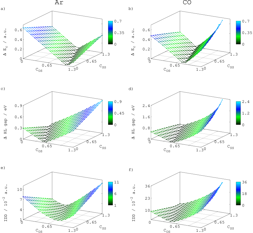
Figure 2: Scans of $\Delta E_{\mathrm{c}}$, $\Delta\mathrm{HL}$ and $\mathrm{IDD}$ with respect to the values of the $c_{\mathrm{OS}}$ and $c_{\mathrm{SS}}$ parameters for the Ar atom (left column) and the CO molecule (right column).

The plots show three main features:

1. For $\Delta E_{\mathrm{c}}$ and $\Delta\mathrm{HL}$ there is no unique pair of $c_{\mathrm{OS}}$ and $c_{\mathrm{SS}}$ values that minimizes the error; on the contrary, it is possible to identify a continuous set of parameter pairs, defined by a linear relation of the type $c_{\mathrm{OS}}=ac_{\mathrm{SS}}+b$, with $a$ and $b$ system– and property–dependent constants, for which the error in minimized. The values on the minimizing line are exactly zero: in fact the plots show the absolute error and the signed error is positive (negative) for small (large) values of $c_{\mathrm{OS}}$. The fact that the error is exactly zero is not surprising because $\Delta E_{\mathrm{c}}$ and $\Delta\mathrm{HL}$ are single–valued quantities, and thus, for a given system and a given property, it is always possible to scale the $c_{\mathrm{OS}}$ and $c_{\mathrm{SS}}$ so that the exact reference values are reproduced.

2. For the $\mathrm{IDD}$, the situation is different. In fact, the $\mathrm{IDD}$ is an integrated quantity which describes how correlation effects are reproduced in the density for all points in space. Thus the error in general is non-zero, because the CCSD(T) reference correlated density is not easily reproduced by a correlation potential which includes only second–order contributions. The plots in the bottom panels of Figure 2 show in fact that the absolute minima can be obtained for $c_{\mathrm{OS}}=0.2$, $c_{\mathrm{SS}}=1.5$ for Argon and $c_{\mathrm{OS}}=0.4$, $c_{\mathrm{SS}}=0.3$ for CO. However, the plots still have a parabolic profile, indicating that for each fixed choice of $c_{\mathrm{SS}}$ a single value of $c_{\mathrm{OS}}$ can be chosen to minimize the $\mathrm{IDD}$ within this constraint.

3. Setting $c_{\mathrm{SS}}=0$ it is possible to find a value of the $c_{\mathrm{OS}}$ parameter such that the error for any given property is close to the absolute minimum. Thus, it is meaningful to consider a scaled–opposite–spin (SOS) second–order OEP method and expect that it may exhibit a performance close to the best achievable by second–order correlation, such approaches can be computationally more favourable and are discussed in the next section.

IV.3 Role of the $c_{\mathrm{OS}}$ parameter in OEP2–SOS methods

In this section we focus our attention on scaled–opposite–spin second–order OEP approaches, which are the most appealing for practical computational applications. We recall in fact that SOS methods provide a computational advantage with respect to other second–order correlation approaches, because when properly implemented they scale as $\mathcal{O}(N^{4})$ rather than as $\mathcal{O}(N^{5})$. In this case, the computationally expensive calculation of the exchange integrals appearing in the SS part is avoided and an efficient $\mathcal{O}(N^{4})$ scaling of the SOS-OEP2 method can be obtained.jung04

In particular, we investigate the performance of the OEP2–SOS correlation methods as a function of the parameter $c_{\mathrm{OS}}$.

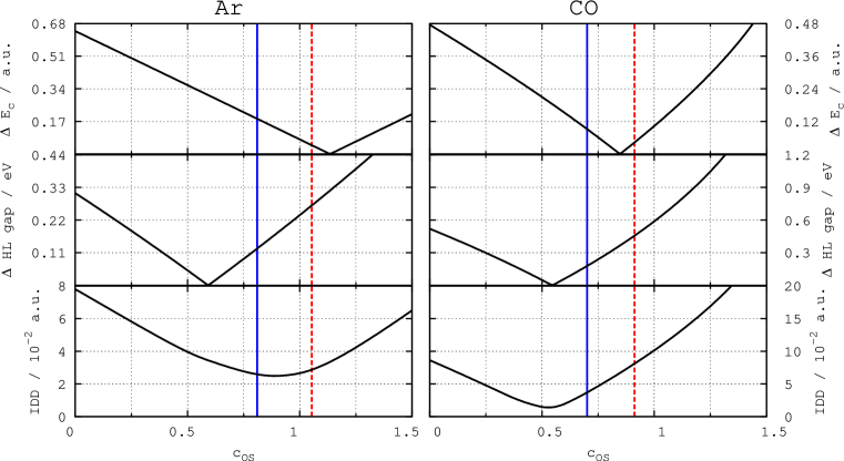
Figure 3: Scans of the errors in several properties (see Section III.1) as obtained from OEP2–SOS approaches with different values of the $c_{\mathrm{OS}}$ parameter, for Ar atom (left panel) and CO (right panel). The red (dashed) and blue vertical lines show the values of $c_{\mathrm{OS}}$ parameter calculated for the OEP2–SOSa and OEP2–SOSb approaches (see Eqs. (21) and (22)), respectively.

Figure 3 reports, for two typical cases, the errors in different properties (see Section III.1 for the definitions of the indicators) as obtained from the OEP2–SOS approach using different values of the $c_{\mathrm{OS}}$ parameter. The figure shows that in all cases a smooth curve is obtained and a single minimum can be well identified for each property. Nevertheless, the minima occur at different values of the $c_{\mathrm{OS}}$ parameter for different systems and properties. Thus, it is not possible to determine with accuracy a single “best” value for the opposite–spin scaling parameter $c_{\mathrm{OS}}$.

As suggested in Ref. 58, a reasonable description of the correlation energy is obtained in most cases by using a system–dependent value of $c_{\mathrm{OS}}$,

$$c_{\mathrm{OS}}^{\mathrm{a}}=\frac{1.3\ E_{\mathrm{OS}}@\mathrm{HF}}{E_{\mathrm{OS}}@\mathrm{OEPx}}\ ,$$ (21)

where $E_{\mathrm{OS}}@\mathrm{HF}$ and $E_{\mathrm{OS}}@\mathrm{OEPx}$ denote the opposite spin part (see Eq.(8)) of the second–order correlation energy expression Eq. (7) computed with Hartree–Fock and OEP exchange–only orbitals, respectively. Using this value of the scaling parameter we can thus define the OEP2-SOSa method (this approach was denoted OEP-SOS in Ref. 58) designed to yield accurate correlation energies. Thus, in the numerator of Eq. (21) we aim to reproduce the reference (CCSD(T)) correlation energy with a noniterative calculation and according to Ref. 87 this can be achieved (approximately) by setting $E_{REF}\approx 1.3E_{OS}@HF$.

On the other hand, analysing the behaviour of different properties as functions of the $c_{OS}$ parameter in several systems, we found that the $c_{\mathrm{OS}}^{\mathrm{a}}$ values are in general too large to achieve an accurate description of the HOMO-LUMO gap and correlated densities. In fact, we found that these are better described using the system-dependent parameter

$$c_{\mathrm{OS}}^{\mathrm{b}}=\frac{E_{\mathrm{OS}}@\mathrm{HF}}{E_{\mathrm{OS}}@\mathrm{OEPx}}\ .$$ (22)

This value of the scaling parameter can thus be used to define the OEP2-SOSb method, which is, by construction, optimized for the description of correlation-potential-related properties.

We note that, there is in practice no additional numerical cost necessary for calculating the value of the $c_{\mathrm{OS}}$ parameter. In fact, as pointed out in Ref. 58, Hartree–Fock and OEPx calculations can be considered as intermediate steps in any OEP2 calculation. We note also that, despite being system dependent, our $c_{OS}$ coefficients define OEP2-SOS methods which are size extensive, because the coefficients are constructed as ratios of two size-extensive quantities (Eqs. (21) and (22)).

IV.4 Assessment of different OEP2-SOS methods

In the previous subsection we saw that it is possible to define two OEP2-SOS approaches, which are expected to work rather accurately for a set of properties. In this section we now assess these methods in a systematic manner to understand their merits and limitations. Moreover, we consider a third approach, namely the OEP2-SOSh method, which is a hybrid of those in Section IV.3. Within the OEP2-SOSh method the self-consistent-field calculations are performed using the $c_{\mathrm{OS}}^{\mathrm{b}}$ coefficient, so that accurate potentials, densities and other one–electron quantities can be obtained, but the final correlation energies are scaled by a factor 1.3, so that they roughly correspond to those of the OEP2-SOSa method obtained with the $c_{\mathrm{OS}}^{\mathrm{a}}$ coefficient.

To start our assessment we report in Table 2 the correlation energies obtained from different OEP approaches and compare them with those from standard correlated methods. Although the correlation energies are defined differently in WFT and KS theories these differences have been shown to be small, see for example Refs. 3; 106. In Table II we make use of this in comparing the WFT MP2 and CCSD(T) correlation energies with those from the OEP approaches investigated in the this work.

Table 2: Correlation energies (m$E_{\mathrm{h}}$) for different systems as obtained from several OEP2, OEP2-SOS, and conventional wave function methods. The last lines report the mean absolute error (MAE), and the mean absolute relative error (MARE) with respect to the CCSD(T) results In each line the best result among OEP2 calculations is highlighted in bold. The last two columns report the SOS coefficients from Eqs. (21) and (22).

	OEP2-						Wavefunction
System	GL2	sc	SOSa	SOSb	SOSh		SOS-MP2	MP2	CCSD(T)		$c_{os}^{a}$	$c_{os}^{b}$
He	-46.24	-35.33	-45.17	-35.42	-46.05		-45.86	-35.28	-40.85		0.997	0.767
Be	nc	-70.76	-96.81	-71.49	-92.94		-88.45	-69.45	-89.35		0.766	0.590
Ne	-457.82	-352.75	-353.31	-269.41	-350.23		-341.71	-345.84	-353.35		1.050	0.808
Mg	-277.20	-209.39	-212.40	-162.42	-211.15		-207.71	-202.27	-214.72		0.977	0.751
Ar	-776.35	-625.70	-594.59	-456.85	-593.91		-591.56	-617.09	-641.00		1.053	0.810
H2	-48.55	-32.20	-42.31	-32.40	-42.11		-41.59	-31.99	-39.72		0.874	0.672
He2	-92.47	-70.66	-92.19	-70.84	-92.09		-91.73	-70.56	-81.70		0.997	0.767
HF	-464.76	-335.67	-339.34	-258.23	-335.70		-325.01	-327.57	-337.29		0.995	0.766
CO	-863.12	-479.81	-518.55	-383.87	-499.03		-456.78	-452.30	-475.78		0.912	0.701
H2O	-466.33	-322.82	-331.08	-251.73	-327.25		-316.95	-314.26	-329.17		0.958	0.737
HCl	-516.48	-384.38	-374.01	-286.92	-373.00		-369.90	-375.10	-402.17		0.975	0.750
Cl2	-1025.12	-748.57	-721.70	-552.04	-717.65		-705.36	-722.49	-770.59		0.967	0.744
N2	-866.33	-496.70	-523.82	-391.91	-509.49		-474.28	-471.54	-491.60		0.885	0.681
Ne2	-915.95	-705.77	-706.77	-538.91	-700.58		-683.53	-691.85	-706.91		1.050	0.808
NH3	-421.59	-290.96	-303.86	-231.85	-301.41		-294.18	-283.97	-305.65		0.941	0.724
C2H6	-693.66	-477.65	-505.89	-386.78	-502.82		-493.57	-462.86	-512.55		0.928	0.714
MAE	148.59a	10.20	15.38	92.90	14.59		19.81	19.87
MARE	35.32%a	4.96%	4.68%	22.53%	4.62%		5.71%	7.11%

nc – not converged.

^a without Be.

Inspection of the table confirms the well known features of the OEP-GL2 method, which yields much too negative correlation energies mori-sanchez:2005:oeppt2 ; engel:2005:oeppt2 , and of the OEP2-sc method, which is instead very accurate in this context bartlett:2005:abinit2 ; grabowski:2007:ccpt2 ; grabowski:2011:jcp . Concerning the OEP2-SOS approaches, we note that, as expected, the OEP2-SOSh method is the most accurate for the correlation energy, yielding a mean absolute error (MAE), calculated with respect to CCSD(T) results, of only 14.59 m$E_{\mathrm{h}}$ and therefore slightly better than that of OEP2-SOSa (15.38 m$E_{\mathrm{h}}$), close to the one of the OEP2-sc method and better than both MP2 and SOS-MP2. On the other hand, as anticipated by the analysis of the previous subsection, an overestimation of the correlation energy is given by the OEP2-SOSb method. Nevertheless, this is almost completely removed when the hybrid OEP2-SOSh method is considered giving also the best mean absolute relative error (4.6%). In the last two columns of Table 2, the SOS coefficients from Eqs. (21) and (22) are reported (note that $c_{\mathrm{OS}}^{\mathrm{a}}=1.3c_{\mathrm{OS}}^{\mathrm{b}}$). We can see that the $c_{\mathrm{OS}}^{\mathrm{a}}$ coefficient is quite system dependent with variation in the range $0.766-1.053$, meaning that a single SOS coefficient, as is used in SOS-MP2 calculations WCMS12 ; grimme03 , cannot yield very accurate results for all systems.

In Table 3 we report the integrated density differences (IDD, see Eq. (20)) corresponding to different OEP2 calculations.

Table 3: Integrated density difference (IDD; Eq. (20)) in units of $10^{-2}$ corresponding to various OEP2 methods. MP2 results are also shown for comparison. The last lines report the mean absolute error (MAE) and the MAE weighted for the number of electrons (MAE/$N_{e}$) In each line the best result for OEP2 or OEP2-SOS calculations is highlighted in bold.

System	OEP-GL2	OEP2-sc	OEP2-SOSa	OEP2-SOSb/h	MP2
He	0.45	0.44	0.42	0.19	0.43
Be	nc	3.13	4.59	1.73	4.30
Ne	14.74	2.66	6.70	2.73	1.53
Mg	5.60	2.20	3.54	4.14	1.80
Ar	5.88	0.75	2.86	2.59	0.36
H2	0.44	0.38	0.24	0.34	0.45
He2	0.35	0.32	0.35	0.57	0.24
HF	6.36	1.65	3.23	1.56	1.79
CO	21.37	2.34	8.10	3.70	1.75
Cl2	13.93	4.11	8.53	5.41	2.19
N2	19.30	1.75	6.99	3.25	1.27
Ne2	6.69	1.73	3.35	4.29	1.13
HCl	4.25	2.28	3.18	2.45	1.27
H2O	5.64	1.47	2.47	1.01	1.50
NH3	3.94	1.01	1.53	0.60	1.03
C2H6	3.49	0.51	1.70	0.95	0.48
MAE	7.50a	1.67	3.61	2.22	1.35
MAE/Ne	0.56a	0.18	0.32	0.19	0.17

nc – not converged.

^a without Be.

The reported IDDs show that the best correlated densities are found by the OEP2-sc approach, while quite large errors are obtained by the original OEP-GL2 method. We note that the OEP2-sc results are, for most systems, in line with those of the MP2 calculations, showing the reasonable accuracy of this functional. A similar accuracy to that of OEP2-sc is observed also for the OEP2-SOSb and OEP2-SOSh results, which yield an MAE of 0.022 and an MAE per electron of 0.002 (note that the two methods coincide for this property) to be compared with the values of 0.017 and 0.002 for OEP2-sc. As expected slightly larger IDD values are obtained for OEP2-SOSa calculations. Nevertheless, we note that the performance of the OEP2-SOSa method is good, being about a factor of two better than the OEP-GL2 method.

Similar trends to those observed for the IDDs are found when the HOMO-LUMO gaps are considered. This is shown in Table 4 where we consider the HOMO-LUMO gap computed by various OEP2 and OEP2-SOS methods and compare them to the benchmark data obtained by direct inversion of the relaxed densities calculated from several ab initio methods.

Table 4: HOMO-LUMO energy gap (eV) for different systems as obtained from several OEP2 and OEP2-SOS approaches. These are compared with those from the KS inversion procedure applied to conventional correlated methods. The last lines report the mean absolute error (MAE), and the mean absolute relative error (MARE) with respect to the CCSD(T) results. In each line the best result for OEP or OEP2-SOS calculations is highlighted in bold.

		OEP2-					Inverse-KS
System	OEPx	GL2	sc	SOSa	SOSb/h		MP2	CCSD(T)
He	21.60	20.95	21.32	20.96	21.11		21.33	21.21
Be	3.57	nc	3.63	3.33	3.50		3.63	3.61
Ne	18.48	14.12	16.45	15.76	16.46		16.81	17.00
Mg	3.18	3.40	3.33	3.37	3.33		3.33	3.36
Ar	11.80	10.95	11.43	11.22	11.37		11.45	11.51
H2	12.09	12.03	12.13	12.04	12.05		12.18	12.14
He2	21.28	20.64	21.02	20.64	20.80		20.68	20.56
HF	11.36	7.80	9.84	9.18	9.74		10.13	10.30
CO	7.77	5.87	7.22	6.79	7.07		7.32	7.29
H2O	8.44	5.99	7.49	7.04	7.41		7.59	7.75
HCl	7.82	7.10	7.52	7.28	7.41		7.60	7.55
Cl2	3.90	2.65	3.35	2.98	3.21		3.32	3.29
N2	9.21	6.73	8.37	7.86	8.22		8.46	8.55
Ne2	17.84	13.49	15.75	15.06	15.76		16.05	16.23
NH3	6.97	5.30	6.35	6.00	6.25		6.41	6.54
C2H6	9.21	8.24	8.85	8.75	8.87		8.82	8.95
MAE	0.52	1.15a	0.21	0.50	0.24		0.10
MARE	6.49$\%$	12.16%a	1.86%	5.20%	2.48%		1.02%

nc – not converged.

^a without Be.

The data in the table show that the best performance is given by the OEP2-sc method, which yields an MAE of 0.21 eV, close to the estimated accuracy of the reference data ($\sim 0.2$ eV). The OEP2-sc method displays a strong improvement with respect to the OEP-GL2 approach, which instead gives a systematic underestimation of the HOMO-LUMO energy gap. A significant improvement with respect to OEP-GL2 is also obtained by considering various scaled-opposite-spin OEP methods. In fact, a reduction of both $c_{\mathrm{SS}}$ and $c_{\mathrm{OS}}$ tends to increase the HOMO-LUMO gap, due to the reduced weight of the correlation contributions in the XC potential. This shows that the scaling of the opposite-spin correlation is an effective way to improve the description of the correlation potential. Accurate results are given in particular by the OEP2-SOSb method (note that for this property OEP2-SOSb and OEP2-SOSh coincide by definition), which yields an MAE of 0.24 eV and an MARE of 2.5%. Slightly larger errors are obtained with the OEP2-SOSa method, which displays a moderate tendency to underestimate the HOMO-LUMO energy gap.

To conclude this section we consider in Figure 4 a direct comparison of the correlation potentials and density differences for several methods. The plots are reported for the Ne, Ar and CO systems and are representative of a general trend.

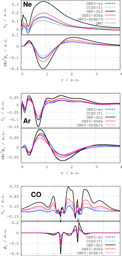
Figure 4: Correlation potential and density contribution, $\rho_{\mathrm{c}}$, for the Ne atom (upper panel), Ar atom (middle panel) and the CO molecule (lower panel), as obtained from different OEP methods as well as benchmark correlated methods and corresponding inverted KS calculations.

Inspection of the figure confirms the observations made above on the behaviour of different functionals. All plots show in fact, the significant overestimation of the correlation potential by the OEP-GL2 method, especially in the valence regions, and the important improvement obtained by considering OEP2-SOS methods. This improvement is, of course, more pronounced for the OEP2-SOSb potential, which is qualitatively comparable with the accurate OEP2-sc one. We observe a systematic improvement of the correlation potentials going from OEP-GL2, through OEP2-SOSa to the OEP2-SOSb/h method which gives the best correlation potentials as compared to the CCSD(T) results. In fact, all methods provide also a qualitatively similar description of the correlated density. Moreover, the OEP2-SOSb and OEP2-sc plots are very close to the CCSD(T) one.

V Conclusions

We have investigated the performance of OEP2-SCS functionals to elucidate the role of the different spin-resolved singly– and doubly–excited contributions, as well as the importance of the independent scaling of such terms. We found that the most important contribution to the description of correlation comes from the doubly excited terms. Moreover, the same- and opposite-spin contributions to the dominant doubly excited terms were found to display a significant proportionality, so that for both the correlation energy and the density-based properties it is possible to individuate a continuous family of OEP2-SCS functionals of high accuracy, differing only in the coefficients used for the the same- and opposite-spin terms. This finding is important because it provides a rationale for the well known scaled-spin-component wave-function approaches, which up to now have been based on empirical observations focusing only on the correlation energy. In addition, the flexibility in the choice of the “best” $c_{\mathrm{OS}}$ and $c_{\mathrm{SS}}$ parameters, clearly suggests that accurate functionals can be defined also in the realm of the scaled-opposite-spin correlation, which is particularly attractive due to its favourable computational cost.

We considered three possible variants of OEP2-SOS functionals, based on different approaches for determining the $c_{\mathrm{OS}}$ parameter, and assessed their performance on a representative set of different systems and properties. Amongst the methods considered, the OEP2-SOSa approach gave the most accurate correlation energies, whereas the OEP2-SOSb method displayed higher accuracy for the description of the electron density, correlation potentials, HOMO-LUMO gaps and orbital energies. Our findings are consistent with similar observations Kronik2014 made for some standard DFT methods which, depending on the choice of the parameters used for defining the XC functional, are either accurate for binding energies or orbital energies, but rarely for both properties at the same time.

Thus, the OEP2-SOSh approach, using a post-SCF rescaling of the correlation energy was constructed as a robust method for the description of correlation energies, correlated densities, and single particle properties; displaying a similar performance to the OEP2-sc method, which is one of the most advanced OEP second-order correlated approaches currently available.

An interesting point in favour of the OEP2-SOS family of functionals is that they display not only improved correlation energies, correlation potentials, HOMO-LUMO gaps and correlated densities but also improved stability in comparison with the OEP-GL2 method. The latter is unbounded from below and can exhibit variational collapse for unphysical exchange–correlation potentials rohr-baerends:2006:oephe ; engel:2005:oeppt2 . However, these potentials do not correspond to KS solutions and can be easily excluded by minimal regularization (such as the truncated SVD approach used in the present work). Nonetheless there can remain difficult cases where the calculations do diverge even with regularization due to the breakdown of the perturbation theory. A prototypical case is the Be atom, for which OEP-GL2 diverges whereas the OEP2-SOS approaches in the present work remain stable for the parameters calculated in SOS-OEP2a ( $c_{\mathrm{OS}}=0.766$) and SOS-OEP2b ( $c_{\mathrm{OS}}=0.590$) ansatzes. Actually the SOS-OEP2 method converges for the whole range of $c_{\mathrm{OS}}$ parameter from $c_{\mathrm{OS}}=0.0$ up to $c_{\mathrm{OS}}=0.770$.

In conclusion, the present work shows that scaled-spin-component, and especially scaled-opposite-spin, methods are promising approaches. This applies not only in the context of ab initio correlated methods, where they are currently increasingly employed in many application and development works, but also in the field of DFT. The availability of OEP2-SOS functionals, which exhibit a favourable computational cost (with respect to similar correlated OEP approaches) and good accuracy, should allow for applications to larger and more complex systems. This will provide a valuable tool for practical studies and, more importantly, a deeper understanding of the behaviour of DFT correlation. This information is essential for the further development of density–functional approximations and may be of utility for improving the quality lower cost of semi-local forms.

VI Acknowledgments

This work was partially supported by the National Science Center under Grants No. DEC-2012/05/N/ST4/02079, DEC-2013/08/T/ST4/00032, and DEC-2013/11/B/ST4/00771, and the European Research Council (ERC) Starting Grant FP7 Project DEDOM, Grant No. 207441. A. M. T. gratefully acknowledges support via the Royal Society University Research Fellowship scheme.

References

- (1) R. M. Dreizler and E. K. U. Gross, Density Functional Theory, Springer, Heidelberg, 1990.
- (2) C. J. Umrigar and X. Gonze, Phys. Rev. A 50, 3827 (1994).
- (3) I. Grabowski, A. M. Teale, S. Śmiga, and R. J. Bartlett, J. Chem. Phys. 135, 114111 (2011).
- (4) H. Eshuis and F. Furche, J. Phys. Chem. Lett. 2, 983 (2011).
- (5) D. Lu, Y. Li, D. Rocca, and G. Galli, Phys. Rev. Lett. 102, 206411 (2009).
- (6) M. Grüning, A. Marini, and A. Rubio, J. Chem. Phys. 124, 154108 (2006).
- (7) E. Fabiano and F. Della Sala, J. Chem. Phys. 126, 214102 (2007).
- (8) D. Langreth and J. Perdew, Solid State Communications 17, 1425 (1975).
- (9) D. C. Langreth and J. P. Perdew, Phys. Rev. B 15, 2884 (1977).
- (10) A. Görling and M. Levy, Phys. Rev. B 47, 13105 (1993).
- (11) W. Kutzelnigg, Int. J. Quantum Chem. 109, 3858 (2009).
- (12) I. Grabowski, S. Hirata, S. Ivanov, and R. J. Bartlett, J. Chem. Phys. 116, 4415 (2002).
- (13) S. Ivanov, S. Hirata, I. Grabowski, and R. J. Bartlett, J. Chem. Phys. 118, 461 (2003).
- (14) I. V. Schweigert, V. F. Lotrich, and R. J. Bartlett, J. Chem. Phys. 125, 104108 (2006).
- (15) R. J. Bartlett, I. Grabowski, S. Hirata, and S. Ivanov, J. Chem. Phys. 122, 034104 (2005).
- (16) A. Görling and M. Levy, Int. J. Quantum Chem. Symp. 29, 93 (1995).
- (17) A. Görling, J. Chem. Phys. 123, 062203 (2005).
- (18) S. Kümmel and L. Kronik, Rev. Mod. Phys. 80, 3 (2008).
- (19) F. Della Sala, Orbital-dependent exact-exchange methods in density functional theory, in Chemical Modelling, vol. 7, edited by M. Springborg, pages 115–161, Royal Society of Chemistry, London, UK, 2011.
- (20) E. Engel and R. M. Dreizler, Orbital functionals: Optimized potential method, in Density Functional Theory, Theor. Math. Phys., pages 227–306, Springer Berlin Heidelberg, 2011.
- (21) A. Görling, Phys. Rev. Lett. 83, 5459 (1999).
- (22) S. Ivanov, S. Hirata, and R. J. Bartlett, Phys. Rev. Lett. 83, 5455 (1999).
- (23) W. Yang and Q. Wu, Phys. Rev. Lett. 89, 143002 (2002).
- (24) A. Heßelmann, A. W. Götz, F. Della Sala, and A. Görling, J. Chem. Phys. 127, 054102 (2007).
- (25) T. Heaton-Burgess, F. A. Bulat, and W. Yang, Phys. Rev. Lett. 98, 256401 (2007).
- (26) J. J. Fernandez, C. Kollmar, and M. Filatov, Phys. Rev. A 82, 022508 (2010).
- (27) M. Städele, J. A. Majewski, P. Vogl, and A. Görling, Phys. Rev. Lett. 79, 2089 (1997).
- (28) S. Sharma, J. K. Dewhurst, C. Ambrosch-Draxl, S. Kurth, N. Helbig, S. Pittalis, S. Shallcross, L. Nordström, and E. K. U. Gross, Phys. Rev. Lett. 98, 196405 (2007).
- (29) M. Betzinger, C. Friedrich, S. Blügel, and A. Görling, Phys. Rev. B 83, 045105 (2011).
- (30) F. Della Sala and A. Görling, J. Chem. Phys. 115, 5718 (2001).
- (31) O. V. Gritsenko and E. J. Baerends, Phys. Rev. A 64, 042506 (2001).
- (32) V. N. Staroverov, G. E. Scuseria, and E. R. Davidson, J. Chem. Phys. 125, 081104 (2006).
- (33) I. G. Ryabinkin, A. A. Kananenka, and V. N. Staroverov, Phys. Rev. Lett. 111, 013001 (2013).
- (34) F. Furche, J. Chem. Phys. 129, 114105 (2008).
- (35) J. Harl and G. Kresse, Phys. Rev. Lett. 103, 056401 (2009).
- (36) X. Ren, A. Tkatchenko, P. Rinke, and M. Scheffler, Phys. Rev. Lett. 106, 153003 (2011).
- (37) A. Heßelmann and A. Görling, Phys. Rev. Lett. 106, 093001 (2011).
- (38) H. Eshuis, J. Bates, and F. Furche, Theor. Chem. Acc. 131, 1 (2012).
- (39) M. Del Ben, J. Hutter, and J. VandeVondele, J. Chem. Theory Comput. 9, 2654 (2013).
- (40) A. Heßelmann and A. Görling, Mol. Phys. 109, 2473 (2011).
- (41) A. Heßelmann and A. Görling, Mol. Phys. 108, 359 (2010).
- (42) M. Hellgren and U. von Barth, Phys. Rev. B 76, 075107 (2007).
- (43) M. Hellgren, D. R. Rohr, and E. K. U. Gross, J. Chem. Phys. 136, 034106 (2012).
- (44) P. Verma and R. J. Bartlett, J. Chem. Phys. 136, 044105 (2012).
- (45) P. Bleiziffer, A. Heßelmann, and A. Görling, J. Chem. Phys. 139, 084113 (2013).
- (46) J. Paier, B. G. Janesko, T. M. Henderson, G. E. Scuseria, A. GrĂĽneis, and G. Kresse, J. Chem. Phys. 132, 094103 (2010).
- (47) J. E. Bates and F. Furche, J. Chem. Phys. 139, (2013).
- (48) A. Grüneis, M. Marsman, J. Harl, L. Schimka, and G. Kresse, J. Chem. Phys. 131, 154115 (2009).
- (49) X. Ren, P. Rinke, G. E. Scuseria, and M. Scheffler, Phys. Rev. B 88, 035120 (2013).
- (50) J. J. Shepherd, A. Grüneis, G. H. Booth, G. Kresse, and A. Alavi, Phys. Rev. B 86, 035111 (2012).
- (51) H. Eshuis and F. Furche, J. Chem. Phys. 136, 084105 (2012).
- (52) E. Fabiano and F. Della Sala, Theor. Chem. Acc. 131, 1 (2012).
- (53) A. Facco Bonetti, E. Engel, R. N. Schmid, and R. M. Dreizler, Phys. Rev. Lett. 86, 2241 (2001).
- (54) P. Mori-Sánchez, Q. Wu, and W. Yang, J. Chem. Phys. 123, 062204 (2005).
- (55) D. Rohr, O. Gritsenko, and E. J. Baerends, Chem. Phys. Lett. 432, 336 (2006).
- (56) H. Jiang and E. Engel, J. Chem. Phys. 123, 224102 (2005).
- (57) I. Grabowski, V. Lotrich, and R. J. Bartlett, J. Chem. Phys. 127, 154111 (2007).
- (58) I. Grabowski, E. Fabiano, and F. Della Sala, Phys. Rev. B 87, 075103 (2013).
- (59) S. Grimme, J. Chem. Phys. 118, 9095 (2003).
- (60) S. Grimme, L. Goerigk, and R. F. Fink, Wiley Interdisciplinary Reviews: Computational Molecular Science 2, 886 (2012).
- (61) R. T. Sharp and G. K. Horton, Phys. Rev. 90, 317 (1953).
- (62) J. D. Talman and W. F. Shadwick, Phys. Rev. A 14, 36 (1976).
- (63) J. B. Krieger, Y. Li, and G. J. Iafrate, Phys. Lett. A 146, 256 (1990).
- (64) S. Kümmel and L. Kronik, Rev. Mod. Phys. 80, 3 (2008).
- (65) E. Engel, Orbital-dependent functional for the exchange-correlation energy: A third generation of dft, in A Primer in Density Functional Theory, edited by C. Fiolhais, F. Nogueira, and M. A. Marques, (Springer, Berlin), 2003.
- (66) S. Ivanov, S. Hirata, and R. J. Bartlett, J. Chem. Phys. 116, 1269 (2002).
- (67) F. Della Sala and A. Görling, J. Chem. Phys. 116, 5374 (2002).
- (68) F. Della Sala and A. Görling, Phys. Rev. Lett. 89, 033003 (2002).
- (69) S. Hirata, S. Ivanov, I. Grabowski, R. J. Bartlett, K. Burke, and J. D. Talman, J. Chem. Phys. 115, 1635 (2001).
- (70) D. P. Joubert, J. Chem. Phys. 127, 244104 (2007).
- (71) C. Kollmar and M. Filatov, J. Chem. Phys. 127, 114104 (2007).
- (72) M. J. G. Peach, J. A. Kattirtzi, A. M. Teale, and D. J. Tozer, J. Chem. Phys. 114, 7179 (2010).
- (73) V. N. Glushkov, S. I. Fesenko, and H. M. Polatoglou, Theor. Chem. Acc. 124, 365 (2009).
- (74) A. Theophilou and V. Glushkov, J. Chem. Phys. 124, 034105 (2006).
- (75) I. Grabowski and V. Lotrich, Mol. Phys. 103, 2087 (2005).
- (76) F. A. Bulat, T. Heaton-Burgess, A. J. Cohen, and W. Yang, J. Chem. Phys. 127, 174101 (2007).
- (77) J. F. Stanton et al., ACES II, Quantum Theory Project, Gainesville, Florida, 2007.
- (78) G. Herzberg, Spectra of Diatomic Molecules, Van Nostrand Reinhold Co., Princeton. N.J., 1970.
- (79) S. Boucier, Spectroscopic Data Relative to Diatomic Molecules, volume 17 of Tables of Constants and Numerical Data, Pergainon Press, Elmsford, N.Y., 1970.
- (80) J. H. Callonion, E. Hirota, K. . Kuchitsu, W. J. Lafferty, A. G. Maki., and C. S. Pote, Landolt-Börnstein: Numerical Data and Function Relationships in Science and Technology, volume 7. h e of Structure Data on Free Polyatomic Molecules, Springer-Verlag, West Berlin, 1976.
- (81) I. Grabowski, A. M. Teale, E. Fabiano, S. Śmiga, A. Buksztel, and F. Della Sala, Molecular Physics 112, 700 (2014).
- (82) P. O. Widmark, P. A. Malmqvist, and B. Roos, Theor. Chim. Acta 77, 291 (1990).
- (83) D. E. Woon and T. H. Dunning, Jr., J. Chem. Phys. 98, 1358 (1993).
- (84) K. A. Peterson and T. H. Dunning, Jr, J. Chem. Phys. 117, 10548 (2002).
- (85) T. H. Dunning, Jr., J. Chem. Phys. 90, 1007 (1989).
- (86) C. Møller and M. S. Plesset, Phys. Rev. 46, 618 (1934).
- (87) Y. Jung, R. C. Lochan, A. D. Dutoi, and M. Head-Gordon, J. Chem. Phys. 121, 9793 (2004).
- (88) G. D. Purvis and R. J. Bartlett, J. Chem. Phys. 76, 1910 (1982).
- (89) G. E. Scuseria, C. L. Janssen, and H. F. Schaefer, J. Chem. Phys. 89, 7382 (1988).
- (90) J. A. Pople, M. Head†Gordon, and K. Raghavachari, J. Chem. Phys. 87, 5968 (1987).
- (91) K. Raghavachari, G. W. Trucks, J. A. Pople, and M. Head-Gordon, Chem. Phys. Lett. 157, 479 (1989).
- (92) N. C. Handy and H. F. Schaefer III, J. Chem. Phys. 81, 5031 (1984).
- (93) J. E. Rice and R. D. Amos, Chem. Phys. Lett. 122, 585 (1985).
- (94) R. J. Bartlett, Analytical evaluation of gradients in coupled-cluster and many-body perturbation theory, in Geometrical Derivatives of Energy Surfaces and Molecular Properties, edited by P. Jørgensen and J. Simons, pages 35–61, Reidel, Dordecht, The Netherlands, 1986.
- (95) E. A. Salter, G. W. Trucks, and R. J. Bartlett, J. Chem. Phys. 90, 1752 (1989).
- (96) T. Helgaker and P. Jørgensen, Theor. Chim. Acta 75, 111 (1989).
- (97) P. Jørgensen and T. Helgaker, J. Chem. Phys. 89, 1560 (1988).
- (98) H. Koch, H. J. A. Jensen, P. Jørgensen, T. Helgaker, G. E. Scuseria, and H. F. Schaefer III, J. Chem. Phys. 92, 4924 (1990).
- (99) K. Hald, A. Halkier, P. Jørgensen, S. Coriani, C. Hättig, and T. Helgaker, J. Chem. Phys. 118, 2985 (2003).
- (100) Q. Wu and W. Yang, J. Chem. Phys. 118, 2498 (2003).
- (101) T. Heaton-Burgess, F. A. Bulat, and W. Yang, Phys. Rev. Lett. 98, 256401 (2007).
- (102) Dalton, a molecular electronic structure program, Release Dalton2013.0 (2013), see http://daltonprogram.org/ .
- (103) K. Aidas et al., WIRES Comput. Mol. Sci. 4, 269 (2014).
- (104) K. Jankowski, K. Nowakowski, I. Grabowski, and J. Wasilewski, J. Chem. Phys. 130, 164102 (2009).
- (105) I. Grabowski, E. Fabiano, and F. Della Sala, Phys. Chem. Chem. Phys. 15, 15485 (2013).
- (106) E. K. U. Gross, M. Petersilka, and T. Grabo, Conventional quantum chemical correlation energy versus density-functional correlation energy, in Density Functional Methods in Chemistry, edited by T. Ziegler, pages 42– 53, ACP, Washington, 1996.
- (107) T. Schmidt, E. Kraisler, A. Makmal, L. Kronik, and S. Kümmel, J. Chem. Phys. 140, 18A510 (2014).