Induced fermionic currents in de Sitter spacetime
in the presence of a compactified cosmic string

Abstract

We investigate the vacuum fermionic currents in the geometry of a compactified cosmic string on background of de Sitter spacetime. The currents are induced by magnetic fluxes running along the cosmic string and enclosed by the compact dimension. We show that the vacuum charge and the radial component of the current density vanish. By using the Abel-Plana summation formula, the azimuthal and axial currents are explicitly decomposed into two parts: the first one corresponds to the geometry of a straight cosmic string and the second one is induced by the compactification of the string along its axis. For the axial current the first part vanishes and the corresponding topological part is an even periodic function of the magnetic flux along the string axis and an odd periodic function of the flux enclosed by the compact dimension with the periods equal to the flux quantum. The azimuthal current density is an odd periodic function of the flux along the string axis and an even periodic function of the flux enclosed by the compact dimension with the same period. Depending on the magnetic fluxes, the planar angle deficit can either enhance or reduce the azimuthal and axial currents. The influence of the background gravitational field on the vacuum currents is crucial at distances from the string larger than the de Sitter curvature radius. In particular, for the geometry of a straight cosmic string and for a massive fermionic field, we show that the decay of the azimuthal current density is damping oscillatory with the amplitude inversely proportional to the fourth power of the distance from the string. This behavior is in clear contrast with the case of the string in Minkowski bulk where the current density is exponentially suppressed at large distances.

PACS numbers: 04.62.+v, 03.70.+k, 98.80.Cq, 11.27.+d

1 Introduction

It is well known that the geometrical and topological effects play a central role in a large number of physical problems. They have important implications on all scales, from subnuclear to cosmological. In particular, in quantum field theory the properties of the vacuum crucially depend on the both geometry and topology of the background spacetime. In the present paper we consider combined effects of the geometry and topology on the vacuum current densities induced by magnetic flux tubes. As a background geometry we consider de Sitter (dS) spacetime and the topological effects are induced by two types of sources. The first one will correspond to a planar angle deficit due to the presence of a cosmic string and the second one comes from the compactification of the spatial dimension along the cosmic string.

The cosmic strings are among the most important types of topological defects that may have been formed by the phase transitions in the early universe [2]. Though the recent observations of the cosmic microwave background radiation have ruled out them as the primary source for primordial density perturbations, the cosmic strings give rise to a number of interesting physical effects such as the doubling images of distant objects or even gravitational lensing, the emission of gravitational waves and the generation of high-energy cosmic rays (see, for instance, [3]). Recent developments on the formation of topological defects in superstring theories have led to a renewed interest in cosmic (super)strings. In particular, a variant of their formation mechanism has been proposed in the framework of brane inflation [4]. String-like defects also appear in a number of condensed matter systems, including liquid crystals and graphene-made structures.

In the simplest theoretical model, the cosmic string is described by a planar angle deficit with the background geometry being locally flat except on the top of the string where it has a delta shaped curvature tensor. The corresponding non-trivial topology induces nonzero vacuum expectation values (VEVs) for physical observables. Specifically, the VEV of the energy-momentum tensor associated with various fields has been developed by many authors [5]-[27]. Moreover, considering a magnetic flux running along the strings, there appear additional contributions to the corresponding vacuum polarization effects for charged fields [9],[28]-[32]. The presence of a magnetic flux induces also vacuum current densities. This phenomenon was analyzed for massless [33] and massive [34] scalar fields. It has been shown that an azimuthal vacuum current appears if the ratio of the magnetic flux by the quantum one has a nonzero fractional part. The analysis of the induced fermionic currents in higher-dimensional cosmic string spacetime in the presence of a magnetic flux have been developed in [35]. The fermionic current induced by a magnetic flux in (2+1)-dimensional conical spacetime and in the presence of a circular boundary has also been analyzed [36].

In general, the analysis of quantum effects for matter fields in a cosmic string spacetime, consider this defect in a flat background geometry. For a cosmic string in a curved background, quantum effects associated with a scalar field have been discussed in [37] for special values of the planar angle deficit. The vacuum polarization in Schwarzschild space-time threaded by an infinite straight cosmic string is investigated in [38]. In recent publications we have investigated the vacuum polarization effects for massive scalar [39] and fermionic [40] fields, induced by a cosmic string in dS spacetime. It has been shown that for massive quantum fields the background gravitational field essentially changes the behavior of the vacuum densities at distances from the string larger than the dS curvature radius, when compared with the case of the string in Minkowski spacetime. Depending on the specific value of the mass, at large distances two regimes are realized with monotonic and oscillatory behavior of the VEVs. Similar analysis for vacuum polarization effects, induced by a cosmic string in anti-de Sitter spacetime, have been developed in [41] and [42] for massive scalar and fermionic fields, respectively.

The choice of dS spacetime as the background geometry in the present paper is motivated by several reasons. First of all, this spacetime is a maximally symmetric solution of the Einstein equation in the presence of a positive cosmological constant and, as a consequence of high degree of symmetry, a large number of physical problems are exactly solvable on its background. As it will be shown below, this is the case for the problem under consideration. The importance of dS spacetime as a gravitational background has essentially increased after the appearance of the inflationary scenario for the expansion of the universe at early stages. Most versions of this scenario assume a period of quasiexponential expansion in which the geometry of the universe is approximated by a portion of dS spacetime. This gives a natural solution to a number of problems in standard cosmology. In addition, the quantum fluctuations in the inflaton field during the inflationary epoch generate inhomogeneities that are seeds for the formation of the large scale cosmic structures. More recently, astronomical observations of high-redshift supernovae, galaxy clusters, and the cosmic microwave background have indicated that at present the universe is accelerating and can be well approximated by the Friedmann-Robertson-Walker cosmological model with the energy dominated by a positive cosmological constant-type source. If the universe is going to accelerate forever, this model will lead asymptotically to a dS spacetime as a future attractor for the dynamics of the universe.

The second type of the topological effects we shall consider here is induced by the compactification of the spatial dimension along the cosmic string axis. The compact spatial dimensions are an inherent feature of most high-energy theories of fundamental physics, including supergravity and superstring theories. An interesting application of the field theoretical models with compact dimensions recently appeared in nanophysics. The long-wavelength description of the electronic states in graphene can be formulated in terms of the Dirac-like theory in three-dimensional spacetime with the Fermi velocity playing the role of speed of light (see, e.g., [43]). In graphene-made structures, like cylindrical and toroidal carbon nanotubes, the background geometry for the corresponding field theory contains one or two compact dimensions. In quantum field theory, the periodicity conditions imposed on the field operator along compact dimensions modify the spectrum for the normal modes and as a result of this the VEVs of physical observables are changed. Recently the analysis of the induced fermionic current and the VEV of the energy-momentum tensor in a compactified cosmic string spacetime in the presence of magnetic flux running along the string, have been developed in [44, 45]. The VEV of the fermionic current in spacetimes with an arbitrary number of toroidally compactified spatial dimensions and in the presence of a constant gauge has been investigated in [46]. Furthermore, the combined effects of topology and the gravitational field on the VEVs of the current density for charged scalar and fermionic fields in the background of dS spacetime with an arbitrary number of toroidally compactified spatial dimensions is considered in [47]. The finite temperature effects on the current densities for scalar and fermionic fields in topologically nontrivial spaces have been discussed in [48, 49].

The present paper is organized as follows. In section 2 we describe the background geometry and construct the complete set of normalized positive- and negative-energy fermionic mode functions obeying a quasiperiodic boundary condition with an arbitrary phase along the string axis. In addition, we assume the presence of a constant gauge field. In section 3, by using the mode-summation method, we first show that the VEVs for the charge density and the radial current vanish. Then we evaluate the renormalized VEV of the azimuthal current density induced by a magnetic flux running along the string axis. It is decomposed into two parts: the first one corresponds to the geometry of a cosmic string in dS spacetime without compactification and the second one is induced by the compactification of the spatial dimension parallel to the string. The VEV of the axial current density is investigated in section 4. This VEV is a purely topological effect induced by the compactification and vanishes in the geometry of a straight cosmic string. The most relevant conclusions of the paper are summarized in section 5. Throughout the paper we use the units with $G=\hbar=c=1$.

2 Geometry of the problem and the fermionic modes

The main objective of this section is to present the geometry of the spacetime, where we develop our analysis and also to obtain the complete set of solutions of Dirac equation in this background. So we first write the line element, in cylindrical coordinates, corresponding to a cosmic string along the $z$-axis in dS spacetime

$$ds^{2}=g_{\mu\nu}dx^{\mu}dx^{\nu}=dt^{2}-e^{2t/\alpha}\left(dr^{2}+r^{2}d\phi^{2}+dz{}^{2}\right)\ ,$$ (2.1)

where $r\geqslant 0$, $t\in(-\infty,+\infty)$ and $0\leqslant\phi\leqslant\phi_{0}$, being $\phi_{0}=2\pi/q$. The parameter $q$, bigger than unity, codifies the presence of the cosmic string. Additionally we shall assume that the direction along the $z$-axis is compactified to a circle with the length $L$: $0\leqslant z\leqslant L$. The parameter $\alpha$ in (2.1) is related to the cosmological constant $\Lambda$ and the scalar curvature $R$ by the expressions $\Lambda=3\alpha^{-2}$ and $R=12\alpha^{-2}$.

In addition to the synchronous time coordinate $t$, we introduce the conformal time $\tau$ according to

$$\tau=-\alpha e^{-t/\alpha}\ ,\ -\infty<\ \tau\ <\ 0\ .$$ (2.2)

In terms of this coordinate, the line element (2.1) is confromally related to the geometry of a cosmic string in Minkowski bulk, with the conformal factor $(\alpha/\tau)^{2}$:

$$ds^{2}=(\alpha/\tau)^{2}\left(d\tau^{2}-dr^{2}-r^{2}d\phi^{2}-dz{}^{2}\right).$$ (2.3)

By the coordinate transformation

$$t=-\alpha\ln f(t_{s},r_{s}),\;r=r_{s}f(t_{s},r_{s})\sin\theta,\;z=r_{s}f(t_{s},r_{s})\cos\theta,$$ (2.4)

and $\phi=\varphi/q$, with the function $f(t_{s},r_{s})=e^{-t_{s}/\alpha}/\sqrt{1-r_{s}^{2}/\alpha^{2}}$, the line element (2.1) is presented in the static form

$$ds^{2}=(1-r_{s}^{2}/\alpha^{2})dt_{s}^{2}-\frac{dr_{s}^{2}}{1-r_{s}^{2}/\alpha^{2}}-r_{s}^{2}(d\theta^{2}+q^{-2}\sin^{2}\theta d\varphi^{2}).$$ (2.5)

This line element has been previously discussed in [50]. It is shown that, to leading order in the gravitational coupling, the effect of the vortex on de Sitter spacetime is described by (2.5).

The dynamics of a massive spinor field in curved spacetime in the presence of a four-vector potential, $A_{\mu}$, is governed by the Dirac equation

$$i\gamma^{\mu}\left(\nabla_{\mu}+ieA_{\mu}~{}\right)\psi-m\psi=0\ ,\mathrm{~{}}\nabla_{\mu}=\partial_{\mu}+\Gamma_{\mu}\ .$$ (2.6)

Here, $\gamma^{\mu}$ represents the Dirac matrix in curved spacetime and $\Gamma_{\mu}$ the spin connection. Both are expressed in terms of the flat space Dirac matrices, $\gamma^{(a)}$, by the relations

$$\gamma^{\mu}=e_{(a)}^{\mu}\gamma^{(a)},\;\Gamma_{\mu}=\frac{1}{4}\gamma^{(a)}\gamma^{(b)}e_{(a)}^{\nu}e_{(b)\nu;\mu}\ ,$$ (2.7)

where the semicolon stands for the standard covariant derivative for vector fields. In (2.7), $e_{(a)}^{\mu}$ is the tetrad basis satisfying the relation $e_{(a)}^{\mu}e_{(b)}^{\nu}\eta^{ab}=g^{\mu\nu}$, with $\eta^{ab}$ being the Minkowski spacetime metric tensor.

We assume that along the compact $z$-dimension the fermionic field obeys the quasiperiodicity condition as shown below:

$$\psi(t,r,\phi,z+L)=e^{2\pi i\beta}\psi(t,r,\phi,z)\ .$$ (2.8)

In the above equation, $\beta$ is a constant phase defined in the interval $[0,\ 1]$. The special cases $\beta=0$ and $\beta=1/2$ correspond to the periodic and antiperiodic boundary conditions (untwisted and twisted fields, respectively). For the rotation around the $z$-axis we shall use the periodic boundary condition

$$\psi(t,r,\phi+\phi_{0},z)=\psi(t,r,\phi,z).$$ (2.9)

For a constant vector potential, $A_{\mu}$, the latter may be excluded from the field equation (2.6) by the gauge transformation

$$A_{\mu}^{\prime}=A_{\mu}+\partial_{\mu}\Lambda,\;\psi^{\prime}=e^{-ie\Lambda}\psi,$$ (2.10)

with $\Lambda=-A_{\mu}x^{\mu}$. The new wave function obeys the equation

$$(i\gamma^{\mu}\nabla_{\mu}-m)\psi^{\prime}=0,$$ (2.11)

and the periodicity conditions

$$\psi^{\prime}(t,r,\phi+\phi_{0},z) = e^{2\pi ia}\psi^{\prime}(t,r,\phi,z),$$ (2.12)

$$\psi^{\prime}(t,r,\phi,z+L) = e^{2\pi i\tilde{\beta}}\psi^{\prime}(t,r,\phi,z),$$ (2.13)

with the notations

$$a=eA_{2}/q,\;\tilde{\beta}=\beta+eA_{3}L/2\pi.$$ (2.14)

Note that the physical components $A_{\phi}$ and $A_{z}$ of the vector potential are related to the covariant components $A_{2}$ and $A_{3}$ by $A_{\phi}=-A_{2}/r$ and $A_{z}=-A_{3}$. The parameters in the phases of the periodicity conditions can be expressed in terms of the magnetic flux along the string axis, $\Phi_{2}=-A_{2}\phi_{0}$, and flux enclosed by the $z$-axis, $\Phi_{3}=-A_{3}L$, by the formulas

$$a=-\Phi_{2}/\Phi_{0},\;\tilde{\beta}=\beta-\Phi_{3}/\Phi_{0},$$ (2.15)

with $\Phi_{0}=2\pi/e$ being the flux quantum. In what follows we will work in terms of the gauge transformed field $\psi^{\prime}$ omitting the prime. The current density is invariant under the gauge transformation (2.10).

Our main interest in this paper is the evaluation of the VEV of the fermionic current density, $j^{\mu}=e\bar{\psi}\gamma^{\mu}\psi$. This VEV is expressed in terms of the two-point function $S_{rs}^{(1)}(x,x^{\prime})=\langle 0|[\psi_{r}(x),\bar{\psi}_{s}(x^{\prime})]|0\rangle$, where $r$ and $s$ are spinor indices and $|0\rangle$ is the vacuum state. For the VEV one has

$$\langle j^{\mu}(x)\rangle\equiv\langle 0|j^{\mu}(x)|0\rangle=-\frac{e}{2}\lim_{x^{\prime}\rightarrow x}\mathrm{Tr}(\gamma^{\mu}S^{(1)}(x,x^{\prime})).$$ (2.16)

In quantum field theory on curved backgrounds the choice of the vacuum is not unique (see, for example, [1]). In dS spacetime there exists a one-parameter family of maximally symmetric quantum states. In what follows we will assume that the field is prepared in the dS-invariant Bunch-Davies vacuum state [52]. In the class of dS-invariant quantum states, the Bunch-Davies vacuum is the only one for which the ultraviolet behavior of the two-point functions is the same as in Minkowski spacetime.

Let $\{\psi_{\sigma}^{(+)}(x),\psi_{\sigma}^{(-)}(x)\}$ be a complete set of normalized solutions to the Dirac equation specified by the set of quantum numbers $\sigma$. Note that the background geometry under consideration is time-dependent and the energy is not conserved. However, we will refer to the solutions $\psi_{\sigma}^{(+)}(x)$ and $\psi_{\sigma}^{(-)}(x)$ as the positive- and negative-energy modes in the sense that in the limit $\alpha\rightarrow\infty$ they reproduce the positive- and negative-energy fermionic modes in Minkowski spacetime. Expanding the field operator in terms of the complete set of fermionic modes, the following mode-sum formula is obtained for the current density:

$$\langle j^{\mu}\rangle=\frac{e}{2}\sum_{\sigma}\left[\bar{\psi}_{\sigma}^{(-)}(x)\gamma^{\mu}\psi_{\sigma}^{(-)}(x)-\bar{\psi}_{\sigma}^{(+)}(x)\gamma^{\mu}\psi_{\sigma}^{(+)}(x)\right].$$ (2.17)

Consequently, in this evaluation we need the fermionic modes for the geometry at hand.

In order to find the mode functions, we will take the flat space Dirac matrices according to [51]

$$\gamma^{(0)}=\left(\begin{array}[]{cc}1&0\\ 0&-1\end{array}\right),\;\gamma^{(a)}=\left(\begin{array}[]{cc}0&\sigma_{a}\\ -\sigma_{a}&0\end{array}\right),$$ (2.18)

where $a=1,2,3$, and $\sigma_{1},\sigma_{2},\sigma_{3}$ are the $2\times 2$ Pauli matrices. The basis of tetrads corresponding to the line element (2.1) may have the form

$$e_{(a)}^{\mu}=e^{-t/\alpha}\left(\begin{array}[]{cccc}e^{t/\alpha}&0&0&0\\ 0&\cos(q\phi)&-\sin(q\phi)/r&0\\ 0&\sin(q\phi)&\cos(q\phi)/r&0\\ 0&0&0&1\end{array}\right).$$ (2.19)

For the curved space gamma matrices, in the coordinate system corresponding to (2.1), this choice leads to the representation

$$\gamma^{0}=\gamma^{(0)},\;\gamma^{l}=e^{-t/\alpha}\left(\begin{array}[]{cc}0&\rho^{l}\\ -\rho^{l}&0\end{array}\right),$$ (2.20)

with the $2\times 2$ matrices

$$\rho^{1}=\left(\begin{array}[]{cc}0&e^{-iq\phi}\\ e^{iq\phi}&0\end{array}\right),\;\rho^{2}=-\frac{i}{r}\left(\begin{array}[]{cc}0&e^{-iq\phi}\\ -e^{iq\phi}&0\end{array}\right),$$ (2.21)

and $\rho^{3}=\sigma_{3}$. For the spin connection components one gets $\Gamma_{0}=0$ and

$$\Gamma_{l}=-\frac{1}{2\alpha}\gamma^{0}\gamma_{l}+\frac{1-q}{2}\gamma^{(1)}\gamma^{(2)}\delta_{l}^{2},$$ (2.22)

for $l=1,2,3$. This leads to the following expression for the combination appearing in the Dirac equation (2.6):

$$\gamma^{\mu}\Gamma_{\mu}=\frac{3\gamma^{0}}{2\alpha}+\frac{1-q}{2r}\gamma^{1}.$$ (2.23)

The positive- and negative-energy mode functions obeying the periodicity conditions (2.13) can be found in a way similar to that we have used in [40] for the geometry of a straight cosmic string in dS spacetime in the absence of the magnetic flux. For the Bunch-Davies vacuum state these functions are given by

$$\psi_{\sigma}^{(\pm)}(x)=C_{\sigma}^{(\pm)}\eta^{2}e^{iq(j+a)\phi+ikz}\left(\begin{array}[]{c}H_{1/2-im\alpha}^{(\lambda_{\pm})}(\gamma\eta)J_{\beta_{1}}(pr)e^{-iq\phi/2}\\ \frac{isp\epsilon_{j}}{\gamma+sk}H_{1/2-im\alpha}^{(\lambda_{\pm})}(\gamma\eta)J_{\beta_{2}}(pr)e^{iq\phi/2}\\ -isH_{-1/2-im\alpha}^{(\lambda_{\pm})}(\gamma\eta)J_{\beta_{1}}(pr)e^{-iq\phi/2}\\ \frac{p\epsilon_{j}}{\gamma+sk}H_{-1/2-im\alpha}^{(\lambda_{\pm})}(\gamma\eta)J_{\beta_{2}}(pr)e^{iq\phi/2}\end{array}\right),$$ (2.24)

where $\lambda_{+}=1$, $\lambda_{-}=2$, $j=\pm 1/2,\pm 3/2,\ldots$, $\eta=|\tau|$, $s=\pm 1$. Moreover, $J_{\nu}(x)$ and $H_{\nu}^{(1,2)}(x)$ are the Bessel and Hankel functions, respectively, and

$$\gamma=\sqrt{{k}^{2}+p^{2}},\;0\leqslant p<\infty.$$ (2.25)

In (2.24), we have defined

$$\beta_{1} = q|j+a|-\epsilon_{j}/2,$$

$$\beta_{2} = q|j+a|+\epsilon_{j}/2,$$ (2.26)

with $\epsilon_{j}=1$ for $j>-a$ and $\epsilon_{j}=-1$ for $j<-a$. The quantum number $j$ determines the eigenvalues of the projection of the total momentum along the cosmic string and the quantum number $s$ corresponds to the eigenvalue of

$$\hat{S}=\gamma^{-1}\Sigma^{n}\hat{p}_{n},\;\Sigma^{n}=\left(\begin{array}[]{cc}\rho^{n}&0\\ 0&\rho^{n}\end{array}\right)$$

where $\hat{p}_{n}=-i\partial_{n}+\delta_{n}^{3}(q-1)\Sigma^{3}/2$ with $n=1,2,3$.

The mode functions above are specified by the complete set of quantum numbers $\sigma=(p,k,j,s)$. In addition, the functions (2.24) obey the periodicity condition (2.12). From the condition (2.13) we find the eigenvalues for the quantum number $k$:

$$k=k_{l}=2\pi(l+{\tilde{\beta}})/L,$$ (2.27)

with $l=0,\pm 1,\pm 2,\ldots$.

The coefficients $C_{\sigma}^{(\pm)}$ are determined by the orthonormalization condition

$$\int d^{3}x\sqrt{g^{(3)}}\psi_{\sigma}^{(\pm)\dagger}\psi_{\sigma^{\prime}}^{(\pm)}=\delta_{\sigma\sigma^{\prime}},$$ (2.28)

where $g^{(3)}$ is the determinant of the spatial metric tensor corresponding to the line element (2.1). The delta symbol in the rhs of (2.28) is understood as the Kronecker delta for the discrete indices $(j,k_{l},s)$ and the Dirac delta function for the continuous one $p\in[0,\ \infty)$. By using the Wronskian for the Hankel functions, we find

$$|C_{\sigma}^{(\pm)}|^{2}=\frac{qpe^{\pm m\alpha\pi}}{16L\alpha^{3}}(\gamma+sk).$$ (2.29)

Note that, if we write the parameter $a$, defined in (2.14), in the form

$$a=n_{0}+a_{0}\ ,\ |a_{0}|<1/2\ ,$$ (2.30)

where $n_{0}$ is an integer number, then, by shifting $j+n_{0}\rightarrow j$, we can see that the VEVs of physical observables depend on $a_{0}$ only.

As it is well known, in Minkowski spacetime, the theory of von Neumann deficiency indices leads to a one-parameter (usually denoted by $\theta$) family of allowed boundary conditions in the background of an Aharonov-Bohm gauge field [53]. Additionally to the regular modes, these boundary conditions, in general, allow normalizable irregular modes. A special case of boundary conditions has been discussed in [54], where the Atiyah-Patodi-Singer type nonlocal boundary condition is imposed at a finite radius, which is then taken to zero. Similar approach, with the MIT bag boundary condition, has been used in [36, 55] for a two-dimensional conical space with a circular boundary. In the geometry under consideration there are no normalizable irregular modes for

$$|a_{0}|\leqslant(1-1/q)/2.$$ (2.31)

In the case $|a_{0}|>(1-1/q)/2$, the irregular mode corresponds to $j=-n_{0}-\mathrm{sgn\,}(a_{0})/2$. For the mode functions (2.24) with this value of the momentum, the boundary condition on the string axis is a special case of one-parameter family of conditions with the parameter $\theta=\pi/2$. Note that with this value and for a massless field both parity and chiral symmetry are conserved [56]. The evaluation of the VEV of the fermionic current for other boundary conditions on the string axis is similar to that described below. The contribution of the regular modes to the VEV is the same for all boundary conditions and the results will differ by the parts related to the irregular modes.

3 Charge, radial and azimuthal currents

Having the complete set of mode functions (2.24), we can evaluate the VEV for the current density by making use of the mode-sum formula (2.17) where now the summation is specified by

$$\sum_{\sigma}=\int_{0}^{\infty}dp\ \sum_{l=-\infty}^{+\infty}\sum_{s=\pm 1}\sum_{j}\ ,$$ (3.1)

with

$$\sum_{j}=\sum_{j=\pm 1/2,\pm 3/2,\cdots}.$$ (3.2)

Of course, the expression in the rhs of (2.17) is divergent and a regularization with the subsequent renormalization is necessary. Here we shall use a cutoff function to regularize without writing it explicitly. The special form of this function will not be important for the further discussion. An alternative way would be the point-splitting regularization procedure which corresponds to the evaluation of the expression under the sign of the limit in (2.16) for $x^{\prime}\neq x$. However, in this case the calculations are more complicated.

First let us consider the charge density:

$$\langle j^{0}\rangle=-\frac{e}{2}\sum_{\sigma}\sum_{\chi=-,+}\chi\psi_{\sigma}^{(\chi)\dagger}(x)\psi_{\sigma}^{(\chi)}(x).$$ (3.3)

Substituting the mode functions (2.24) and using the relation [57]

$$H_{\nu}^{(2)}(x)=\frac{2i}{\pi}e^{i\pi\nu/2}K_{\nu}(ix),$$ (3.4)

with $K_{\nu}(x)$ being the MacDonald function, we obtain

$$\langle j^{0}\rangle = -\frac{eq\eta^{4}}{4\pi^{2}L\alpha^{3}}\int_{0}^{\infty}dp\,p\sum_{l=-\infty}^{+\infty}\gamma\sum_{j}\left[J_{\beta_{1}}^{2}(pr)+J_{\beta_{2}}^{2}(pr)\right]$$ (3.5)

$$\times\sum_{\chi=-,+}\chi\left[|K_{1/2+\chi im\alpha}(i\gamma\eta)|^{2}+|K_{-1/2+\chi im\alpha}(i\gamma\eta)|^{2}\right].$$

By taking into account that $K_{-\nu}(x)=K_{\nu}(x)$, we conclude that the charge density vanishes.

For the VEV of the radial current density one has

$$\langle j^{1}\rangle=-\frac{e}{2}\sum_{\sigma}\sum_{\chi=-,+}\chi\psi_{\sigma}^{(\chi)\dagger}(x)\gamma^{0}\gamma^{1}\psi_{\sigma}^{(\chi)}(x).$$ (3.6)

Substituting the corresponding gamma matrices and the fermionic mode functions from (2.24), it can be shown that all terms cancel and the resulting radial current is also zero.

Now we turn to the azimuthal current which is given by the expression (2.17) with $\mu=2$. Substituting (2.24), we can see that the positive- and negative-energy modes give the same contribution. By using (3.4), and after the summation over $s$, the VEV of the azimuthal current is presented in the form

$$\langle j^{2}\rangle=-\frac{2eq\eta^{5}}{\pi^{2}L\alpha^{4}r}\int_{0}^{\infty}dp\,p^{2}\sum_{j}\epsilon_{j}J_{\beta_{1}}(pr)J_{\beta_{2}}(pr)\sum_{l=-\infty}^{+\infty}\mathrm{Re\,}\left[K_{1/2+im\alpha}(i\gamma\eta)K_{1/2+im\alpha}(-i\gamma\eta)\right].$$ (3.7)

In order to separate explicitly the topological part, for the summation over $l$, we apply the Abel-Plana formula in the form [58, 59]

$$\frac{2\pi}{L}\sum_{l=-\infty}^{\infty}g(k_{l})f(|k_{l}|)=\int_{0}^{\infty}du\,\left[g(u)+g(-u)\right]f(u)$$

$$\qquad+i\int_{0}^{\infty}du\left[f(iu)-f(-iu)\right]\sum_{\chi=\pm 1}\frac{g(i\chi u)}{e^{Lu+2\pi i\chi\tilde{\beta}}-1}\ ,$$ (3.8)

choosing $g(u)=1$ and

$$f(u)=\mathrm{Re\,}[K_{1/2+im\alpha}(i\eta\sqrt{u^{2}+p^{2}})K_{1/2+im\alpha}(-i\eta\sqrt{u^{2}+p^{2}})].$$ (3.9)

The first term in the rhs of (3.8) is responsible for the azimuthal current in the cosmic string background without compactification, that will be denoted below by $\left\langle j^{2}\right\rangle_{s}$. The second one corresponds to the contribution due to the compactification of the string along the $z$-axis, denoted by $\left\langle j^{2}\right\rangle_{c}$. Therefore, the application of the summation formula (3.8) allows us to decompose the azimuthal current as

$$\left\langle j^{2}\right\rangle=\left\langle j^{2}\right\rangle_{s}+\left\langle j^{2}\right\rangle_{c}.$$ (3.10)

As we shall see, the compactified part goes to zero in the limit $L\rightarrow\infty$.

We start the evaluation with the part corresponding to the geometry of a straight cosmic string, $\left\langle j^{2}\right\rangle_{s}$. Using the first term in the Abel-Plana formula, for this part we get

$$\left\langle j^{2}\right\rangle_{s} = -\frac{2eq\eta^{5}}{r\pi^{3}\alpha^{4}}\int_{0}^{\infty}dp\,p^{2}\int_{0}^{\infty}dk\sum_{j}\epsilon_{j}J_{\beta_{1}}(pr)J_{\beta_{2}}(pr)$$ (3.11)

$$\times\mathrm{Re\,}\left[K_{1/2+im\alpha}(i\gamma\eta)K_{1/2+im\alpha}(-i\gamma\eta)\right],$$

where $\gamma$ is given by the expression (2.25). Replacing the product of the MacDonald functions by the integral representation [60]

$$K_{\nu}(ix)K_{\nu}(-ix)=\int_{0}^{\infty}duu^{-1}\int_{0}^{\infty}dy\cosh{(2\nu y)}\exp\left[-2ux^{2}\sinh^{2}y-1/(2u)\right],$$ (3.12)

the integral over $k$ is evaluated directly. Performing the integral over $p$ with the help of the formula below [61]

$$\int_{0}^{\infty}dp\,p^{2}e^{-bp^{2}}J_{\beta_{1}}(pr)J_{\beta_{2}}(pr)=r\epsilon_{j}\frac{e^{-r^{2}/2b}}{4b^{2}}\left[I_{\beta_{1}}(r^{2}/2b)-I_{\beta_{2}}(r^{2}/2b)\right],$$ (3.13)

we obtain

$$\left\langle j^{2}\right\rangle_{s} = -\frac{\sqrt{2}eq\eta^{5}}{r^{5}\pi^{5/2}\alpha^{4}}\int_{0}^{\infty}dy\,\cosh y\cos(2m\alpha y)$$ (3.14)

$$\times\int_{0}^{\infty}dz\,z^{3/2}e^{-z\left[1+2(\eta/r)^{2}\sinh^{2}y\right]}\mathcal{J}(q,a_{0},z),$$

where we have introduced the notation

$$\mathcal{J}(q,a_{0},z)=\sum_{j}\left[I_{\beta_{1}}(z)-I_{\beta_{2}}(z)\right].$$ (3.15)

The integration over $y$ in (3.14) can be done explicitly and one finds

$$\left\langle j^{2}\right\rangle_{s}=-\frac{eq\alpha^{-4}}{\sqrt{2}\pi^{5/2}}\int_{0}^{\infty}dx\,x^{3/2}e^{x(1-r^{2}/\eta^{2})}\mathcal{J}(q,a_{0},xr^{2}/\eta^{2})\,\mathrm{Re\,}\left[K_{1/2+im\alpha}(x)\right],$$ (3.16)

where we have introduced a new integration variable $x=z\eta^{2}/r^{2}$. The current density given by this formula is a periodic odd function of the flux along the string axis with the period equal to the flux quantum. The azimuthal current density, given by (3.16), depends on the radial and time coordinates through the ratio $r/\eta$. This property is a consequence of the maximal symmetry of dS spacetime and the Bunch-Davies vacuum. By taking into account that the combination $r_{p}=\alpha r/\eta$ is the proper distance from the string, we see that $r/\eta$ is the proper distance measured in units of the dS curvature scale $\alpha$.

For the further transformation of the expression in the rhs of (3.16), we follow the procedure used in [36] for the summation over $j$ in (3.15). Introducing the notation

$$\mathcal{I}(q,a_{0},z)=\sum_{j}I_{\beta_{1}}(z),$$ (3.17)

we can see that $\sum_{j}I_{\beta_{2}}(z)=\mathcal{I}(q,-a_{0},z)$. For the series (3.17) one has the integral representation

$$\mathcal{I}(q,a_{0},z)=\frac{e^{z}}{q}-\frac{1}{\pi}\int_{0}^{\infty}dx\frac{e^{-z\cosh x}f(q,a_{0},x)}{\cosh(qx)-\cos(q\pi)}$$

$$\qquad+\frac{2}{q}\sum_{k=1}^{p}(-1)^{k}\cos[2\pi k(a_{0}-1/(2q))]e^{z\cos(2\pi k/q)},$$ (3.18)

in which $p$ is an integer defined by $2p<q<2p+2$ and

$$f(q,a_{0},x)=\sum_{\chi=-,+}\chi\cos\left[q\pi\left(1/2-\chi a_{0}\right)\right]\cosh\left[\left(qa_{0}+\chi q/2-1/2\right)x\right]\ .$$ (3.19)

In the specific case $q=2p$, the term

$$-(-1)^{q/2}\frac{e^{-z}}{q}\sin{(q\pi a_{0})}$$ (3.20)

should be added to the rhs of (3.18). By taking into account (3.18), for the function (3.15) one gets

$$\mathcal{J}(q,a_{0},z) = \frac{4}{\pi}\int_{0}^{\infty}dx\frac{e^{-z\cosh(2x)}g(q,a_{0},2x)\cosh x}{\cosh(2qx)-\cos(q\pi)}$$ (3.21)

$$+\frac{4}{q}\sum_{k=1}^{p}(-1)^{k}\sin\left(\pi k/q\right)\sin\left(2\pi ka_{0}\right)e^{z\cos(2\pi k/q)},$$

where

$$g(q,a_{0},x)=\sum_{\chi=-,+}\chi\cos\left[q\pi\left(1/2+\chi a_{0}\right)\right]\cosh\left[\left(1/2-\chi a_{0}\right)qx\right].$$ (3.22)

In the case $q=2p$, the term $-2(-1)^{q/2}(e^{-z}/q)\sin{(q\pi a_{0})}$ must be added to the rhs of (3.21). As is seen, in the absence of a magnetic flux along the string, $a_{0}=0$, one has $\mathcal{J}(q,0,z)=0$ and the azimuthal current density $\left\langle j^{2}\right\rangle_{s}$ vanishes which is the same result as for the flat space in the presence of the cosmic string [44].

The azimuthal current density in dS spacetime induced by the magnetic flux is obtained as a special case with $q=1$. In this case, for the function in the integrand of (3.21) one has

$$g(1,a_{0},2x)=-2\sin(\pi a_{0})\cosh(2a_{0}x)\cosh x,$$ (3.23)

and the sum in the rhs of (3.21) is absent. For the function $\mathcal{J}(q,a_{0},z)$ one gets

$$\mathcal{J}(1,a_{0},z)=-\frac{2}{\pi}\sin(\pi a_{0})\int_{0}^{\infty}du\,e^{-z\cosh u}\cosh(a_{0}u).$$ (3.24)

As a result, in the absence of the planar angle deficit the expression for the azimuthal current density is simplified to

$$\left\langle j^{2}\right\rangle_{s} = 2\sqrt{2}\frac{e\sin(\pi a_{0})}{\pi^{7/2}\alpha^{4}}\int_{0}^{\infty}du\,\cosh(2a_{0}u)$$ (3.25)

$$\times\int_{0}^{\infty}dx\,x^{3/2}e^{x[1-2(r/\eta)^{2}\cosh^{2}u]}\,\mathrm{Re\,}\left[K_{1/2+im\alpha}(x)\right].$$

An equivalent expression for the azimuthal current in general case of $q$ is obtained substituting (3.21) into (3.14) and integrating over $z$:

$$\left\langle j^{2}\right\rangle_{s} = -\frac{3e}{4\pi^{2}(\alpha r/\eta)^{4}}\int_{0}^{\infty}du\,\cos(2m\alpha\,\mathrm{arcsinh\,}(ur/\eta))$$ (3.26)

$$\times\left[\frac{q}{\pi}\int_{0}^{\infty}dx\frac{g(q,a_{0},2x)\cosh x}{\cosh(2qx)-\cos(q\pi)}\left(\cosh^{2}x+u^{2}\right)^{-5/2}\right.$$

$$\left.+\sum_{k=1}^{p}\frac{(-1)^{k}\sin\left(\pi k/q\right)\sin\left(2\pi ka_{0}\right)}{\left[\sin^{2}(\pi k/q)+u^{2}\right]^{5/2}}\right],$$

where we have made the change of variables $u=(\eta/r)\sinh y$. In the absence of the conical defect one has $q=1$ and from (3.26) we find a simpler formula

$$\left\langle j^{2}\right\rangle_{s}=\frac{3e\sin(\pi a_{0})}{4\pi^{3}\alpha^{4}}\int_{0}^{\infty}du\,\cosh(2a_{0}u)\int_{0}^{\infty}dx\,\frac{\cos(2m\alpha\,\mathrm{arcsinh\,}x)}{[x^{2}+(r/\eta)^{2}\cosh^{2}u]^{5/2}}.$$ (3.27)

For a massless field, integrating over $u$, from the general formula (3.26) we find

$$\left\langle j^{2}\right\rangle_{s} = -\frac{e}{2\pi^{2}(\alpha r/\eta)^{4}}\left[\sum_{k=1}^{p}\frac{(-1)^{k}\sin\left(2\pi ka_{0}\right)}{\sin^{3}(\pi k/q)}\right.$$ (3.28)

$$+\left.\frac{q}{\pi}\int_{0}^{\infty}dx\,\frac{g(q,a_{0},2x)\cosh^{-3}x}{\cosh(2qx)-\cos(q\pi)}\right].$$

The above result shows that $\left\langle j^{2}\right\rangle_{s}$ is conformally related to the corresponding induced current in pure cosmic string spacetime [44], with the conformal factor $\left(\eta/\alpha\right)^{4}$, as expected.

In the region near the string, $r/\eta\ll 1$, the dominant contribution to (3.16) comes from large $x$ and we can use the asymptotic expression of the MacDonald function for large arguments. The leading term is independent of the mass and it reduces to (3.28) which diverges on the string with the inverse fourth power of the proper distance. At large distances from the string, $r/\eta\gg 1$, in (3.16) we use the asymptotic form of the MacDonald function for small values of the argument. The leading term in the asymptotic expansion of the azimuthal current behaves as

$$\left\langle j^{2}\right\rangle_{s}\propto\frac{\cos\left[2m\alpha\ln(r/\eta)+\theta\right]}{(\alpha r/\eta)^{4}},$$ (3.29)

with a phase $\theta$ depending on the parameters $m\alpha$, $q$ and $a_{0}$. As a result, at large distances the azimuthal current in the geometry of a straight cosmic string damps oscillatory with the amplitude decaying as the inverse fourth power of the proper distance from the string. The oscillation frequency increases with increasing mass. In the region under consideration the influence of the gravitational field on the current density is essential. The behavior of the current density in dS spacetime, described by (3.29), is crucially different from that for the string in Minkowski bulk. In the latter case, at large distances from the string the current density for a massive field is suppressed exponentially, by the factor $e^{-2mr\sin(\pi/q)}$ for $q\geqslant 2$ and by the factor $e^{-2mr}$ for $q<2$.

In the left panel of figure 1 we have plotted the quantity $r_{p}^{4}\left\langle j^{2}\right\rangle_{s}/e$, with $r_{p}=\alpha r/\eta$ being the proper distance from the string, as a function of the ratio $r/\eta$ (proper distance measured in units of $\alpha$) for $a_{0}=1/4$ and for separate values of the parameter $q$ (the numbers near the curves). The full curves correspond to a massive field with $m\alpha=1$ and the dashed lines are for a massless field. In the latter case the combination $r_{p}^{4}\left\langle j^{2}\right\rangle_{s}$ does not depend on $r/\eta$. From the asymptotic analysis given above it follows that $r_{p}^{4}\left\langle j^{2}\right\rangle_{s}|_{r=0}=r_{p}^{4}\left\langle j^{2}\right\rangle_{s}|_{m=0}$ which is also seen from the graphs. For large values of $r/\eta$ and for a massive field we see the characteristic oscillations described by (3.29). In the right panel of figure 1 the quantity $r_{p}^{4}\left\langle j^{2}\right\rangle_{s}/e$ is displayed as a function of the parameter $a_{0}$ for fixed values $r/\eta=1$ (full curves) and $r/\eta=5$ (dashed curves). Again, the numbers near the full curves correspond to the values of $q$ and we have taken $m\alpha=1$. For the dashed curves the same values of $q$ are used and $|\left\langle j^{2}\right\rangle_{s}|$ increases with increasing $q$.

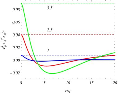
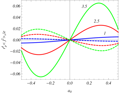
Figure 1: The azimuthal current in the geometry of a straight cosmic string, multiplied by $r_{p}^{4}$, as a function of the distance from the string (left panel) and as a function of the parameter $a_{0}$ (right panel) for separate values of $q$ (numbers near the curves). On the left panel the graphs are plotted for $a_{0}=1/4$. The full curves correspond to a massive field with $m\alpha=1$ and the dashed curves are for a massless field. On the right panel the graphs are plotted for fixed values of $r/\eta=1$ (full curves) and $r/\eta=5$ (dashed curves).

Now, we turn to the part in the azimuthal current density induced by the compactification of the string along its axis. Using the second term in the rhs of the Abel-Plana formula, from (3.7) we obtain

$$\langle j^{2}\rangle_{c} = \frac{eq\eta^{5}}{\pi^{3}\alpha^{4}r}\int_{0}^{\infty}dp\,p^{2}\sum_{j}\epsilon_{j}J_{\beta_{1}}(pr)J_{\beta_{2}}(pr)\int_{p}^{\infty}dk\,\sum_{\chi=\pm 1}\frac{1}{e^{Lk+2\pi i\chi\tilde{\beta}}-1}$$ (3.30)

$$\times\mathrm{Im\,}\left\{K_{1/2+im\alpha}(\eta\lambda)\left[K_{1/2+im\alpha}(e^{\pi i}\eta\lambda)-K_{1/2+im\alpha}(e^{-\pi i}\eta\lambda)\right]\right\}.$$

where $\lambda=\sqrt{k^{2}-p^{2}}$. By employing the relation [57]

$$K_{\nu}(e^{im\pi}z)=e^{-im\nu\pi}K_{\nu}(z)-i\pi\frac{\sin(m\nu\pi)}{\sin(\nu\pi)}I_{\nu}(z),$$ (3.31)

we can see that

$$K_{\nu}(e^{i\pi}z)-K_{\nu}(e^{-i\pi}z)=-\pi i\left[I_{-\nu}(z)+I_{\nu}(z)\right].$$ (3.32)

Hence, for the topological part we obtain

$$\langle j^{2}\rangle_{c} = -\frac{2eq\eta^{5}}{\pi^{2}\alpha^{4}r}\sum_{l=1}^{\infty}\cos(2\pi\tilde{\beta}l)\int_{0}^{\infty}dp\,p^{2}\sum_{j}\epsilon_{j}J_{\beta_{1}}(pr)J_{\beta_{2}}(pr)\int_{0}^{\infty}d\lambda\,\lambda$$ (3.33)

$$\times\frac{e^{-lL\sqrt{\lambda^{2}+p^{2}}}}{\sqrt{\lambda^{2}+p^{2}}}\mathrm{Re\,}\left\{K_{1/2+im\alpha}(\eta\lambda)\left[I_{-1/2-im\alpha}(\eta\lambda)+I_{1/2+im\alpha}(\eta\lambda)\right]\right\},$$

where we have used the expansion $\left(e^{u}-1\right)^{-1}=\sum_{l=1}^{\infty}e^{-lu}$.

For the further transformation we employ the integral representation (see also [49])

$$\frac{e^{-lL\sqrt{\lambda^{2}+p^{2}}}}{\sqrt{\lambda^{2}+p^{2}}}=\frac{2}{\sqrt{\pi}}\int_{0}^{\infty}ds\,e^{-(\lambda^{2}+p^{2})s^{2}-l^{2}L^{2}/4s^{2}}.$$ (3.34)

Substituting into (3.33) and changing the order of integrations, the integral over $p$ is evaluated by making use of (3.13). For the integral over $\lambda$ we use the formula

$$\int_{0}^{\infty}d\lambda\,\lambda e^{-\lambda^{2}s^{2}}K_{\nu}(\eta\lambda)\left[I_{-\nu}(\eta\lambda)+I_{\nu}(\eta\lambda)\right]=\frac{1}{2s^{2}}e^{\eta^{2}/2s^{2}}K_{\nu}(\eta^{2}/2s^{2}).$$ (3.35)

The latter is obtained from the formula [61]

$$\int_{0}^{\infty}d\lambda\,\lambda e^{-\lambda^{2}s^{2}}I_{\nu}^{2}(\eta\lambda)=\frac{1}{2s^{2}}e^{\eta^{2}/2s^{2}}I_{\nu}(\eta^{2}/2s^{2}),$$ (3.36)

by taking into account the relation between the functions $K_{\nu}(x)$ and $I_{\pm\nu}(x)$.

As a result, for the topological contribution in the azimuthal current density we get

$$\langle j^{2}\rangle_{c} = -\frac{\sqrt{2}eq}{\pi^{5/2}\alpha^{4}}\sum_{l=1}^{\infty}\cos(2\pi\tilde{\beta}l)\int_{0}^{\infty}dx\,x^{3/2}e^{x[1-r^{2}/\eta^{2}-l^{2}L^{2}/(2\eta^{2})]}$$ (3.37)

$$\times\mathcal{J}(q,a_{0},xr^{2}/\eta^{2})\,\mathrm{Re\,}\left[K_{1/2+im\alpha}(x)\right],$$

with the new integration variable $x=\eta^{2}/(2s^{2})$ and with the function $\mathcal{J}(q,a_{0},z)$ given by (3.21). As is seen from this expression, the topological part in the azimuthal current density is a periodic odd function of the magnetic flux along the string and a periodic even function of the flux enclosed by the compactified dimension. In both cases, the period is equal to the flux quantum. By taking into account the expression (3.16), the total azimuthal current is written in the form

$$\langle j^{2}\rangle = -\frac{\sqrt{2}eq}{\pi^{5/2}\alpha^{4}}\sideset{}{{}^{\prime}}{\sum}_{l=0}^{\infty}\cos(2\pi\tilde{\beta}l)\int_{0}^{\infty}dx\,x^{3/2}e^{x[1-r^{2}/\eta^{2}-l^{2}L^{2}/(2\eta^{2})]}$$ (3.38)

$$\times\mathcal{J}(q,a_{0},xr^{2}/\eta^{2})\,\mathrm{Re\,}\left[K_{1/2+im\alpha}(x)\right],$$

where the prime on the sign of the summation means that the term $l=0$ should be taken with the coefficient 1/2. The latter corresponds to $\langle j^{2}\rangle_{s}$. The azimuthal current density depends on $L$, $r$, and $\eta$ through the ratios $L/\eta$ and $r/\eta$ which are the proper length of the compact dimension and proper distance from the string axis measured in units of $\alpha$. Again, this feature is a consequence of the maximal symmetry of dS spacetime. In the absence of the planar angle deficit one has $q=1$ and, by using (3.24), the general formula (3.38) is reduced to the expression

$$\langle j^{2}\rangle = \frac{4\sqrt{2}e}{\pi^{7/2}\alpha^{4}}\sin(\pi a_{0})\sideset{}{{}^{\prime}}{\sum}_{l=0}^{\infty}\cos(2\pi\tilde{\beta}l)\int_{0}^{\infty}du\,\cosh(2a_{0}u)\,$$ (3.39)

$$\times\int_{0}^{\infty}dx\,x^{3/2}e^{x[1-2(r/\eta)^{2}\cosh^{2}u-l^{2}L^{2}/(2\eta^{2})]}\,\mathrm{Re\,}\left[K_{1/2+im\alpha}(x)\right].$$

The latter presents the azimuthal current induced by an infinitely thin flux tube along the compactified $z$-axis.

For a massless field, by taking into account that $K_{1/2}(x)=e^{-x}\sqrt{\pi/2x}$ and using (3.21), the integration over $x$ in (3.38) is done explicitly and one finds

$$\langle j^{2}\rangle = -\frac{16\pi^{-2}e}{(\alpha/\eta)^{4}}\sideset{}{{}^{\prime}}{\sum}_{l=0}^{\infty}\cos(2\pi\tilde{\beta}l)\left[\sum_{k=1}^{p}\frac{(-1)^{k}\sin\left(\pi k/q\right)\sin\left(2\pi ka_{0}\right)}{[4r^{2}\sin^{2}(\pi k/q)+l^{2}L^{2}]^{2}}\right.$$ (3.40)

$$+\left.\frac{q}{\pi}\int_{0}^{\infty}dx\frac{g(q,a_{0},2x)\cosh x}{\cosh(2qx)-\cos(q\pi)}(4r^{2}\cosh^{2}x+l^{2}L^{2})^{-2}\right]\,.$$

In this case the azimuthal current is equal to $(\eta/\alpha)^{4}$ times the one for the flat space in the presence of the compactified cosmic string [44].

Let us discuss the behavior of the topological part in the azimuthal current in the asymptotic regions of the parameters. First we consider the region near the cosmic string. From (3.15) it follows that in the limit $z\rightarrow 0$, to the leading order one has

$$\mathcal{J}(q,a_{0},z)\approx-\frac{\mathrm{sgn\,}(a_{0})(z/2)^{q(1/2-|a_{0}|)-1/2}}{\Gamma(q(1/2-|a_{0}|)+1/2)}.$$ (3.41)

Substituting this into (3.37), to the same order for the topological contribution we get

$$\langle j^{2}\rangle_{c} = \frac{\mathrm{sgn\,}(a_{0})\sqrt{2}eq(r/\sqrt{2}\eta)^{q(1-2|a_{0}|)-1}}{\pi^{5/2}\alpha^{4}\Gamma(q(1/2-|a_{0}|)+1/2)}\sum_{l=1}^{\infty}\cos(2\pi\tilde{\beta}l)$$ (3.42)

$$\times\int_{0}^{\infty}dx\,x^{q(1/2-|a_{0}|)+1}e^{x[1-l^{2}L^{2}/(2\eta^{2})]}\,\mathrm{Re\,}\left[K_{1/2+im\alpha}(x)\right].$$

From here it follows that the topological part in the azimuthal current vanishes on the string for $|a_{0}|<(1-1/q)/2$, is finite for $|a_{0}|=(1-1/q)/2$ and diverges for $|a_{0}|>(1-1/q)/2$. Note that in the latter case the divergent contribution comes from the irregular mode. For $a_{0}\neq 0$, in the region near the string the total current is dominated by the part $\left\langle j^{2}\right\rangle_{s}$.

For large values $r$, $r/\eta\gg 1$, the dominant contribution to the integral in (3.38) comes from the values of $x$ in the region $x\lesssim\eta^{2}/r^{2}$ and we replace the MacDonald function by its asymptotic form for small values of the argument. At large distances, the behavior of the azimuthal current density depends crucially on whether the parameter $\tilde{\beta}$ is zero or not. For $0<\tilde{\beta}<1$, we use the relation

$$\sideset{}{{}^{\prime}}{\sum}_{l=0}^{\infty}\cos(2\pi\tilde{\beta}l)e^{-yl^{2}L^{2}/(2r^{2})}\approx\frac{r}{L}\sqrt{\frac{\pi}{2y}}e^{-2(\pi\sigma_{\beta}r/L)^{2}/y},$$ (3.43)

valid for $L/r\ll 1$, with $\sigma_{\beta}=\min(\tilde{\beta},1-\tilde{\beta})$ and $y=xr^{2}/\eta^{2}$. For $q\geqslant 2$ the main contribution comes from the term $k=1$ in the expression (3.21) for the function $\mathcal{J}(q,a_{0},z)$. The remaining integral is expressed in terms of the MacDonald function with the large argument. By using the corresponding asymptotic expression, to the leading order one finds

$$\langle j^{2}\rangle \approx \frac{2e\sigma_{\beta}\eta^{2}/L^{2}}{\alpha^{4}\left(r/\eta\right)^{2}}\frac{\sin\left(2\pi a_{0}\right)}{\sin(\pi/q)}\frac{e^{-4\pi\sigma_{\beta}r\sin(\pi/q)/L}}{\sqrt{\cosh(\pi m\alpha)}}\,$$ (3.44)

$$\times\cos\left[m\alpha\ln\left(\frac{2rL\sin(\pi/q)}{\pi\sigma_{\beta}\eta^{2}}\right)+\beta_{0}(m\alpha)\right],$$

where $\beta_{0}$ is the phase of the function $\Gamma(1/2+im\alpha)$. Hence, for $\tilde{\beta}\neq 0$ at large distances the topological part in the current density is exponentially small. In the case $q<2$ the suppression is stronger, by the factor $e^{-4\pi\sigma_{\beta}r/L}$.

At large distances, $r/\eta\gg 1$, and for $\tilde{\beta}=0$, in (3.38) the dominant contribution to the series comes from large $l$ and we use the asymptotic formula

$$\sideset{}{{}^{\prime}}{\sum}_{l=0}^{\infty}e^{-yl^{2}L^{2}/(2r^{2})}\approx\frac{r}{L}\sqrt{\frac{\pi}{2y}}.$$ (3.45)

The MacDonald function is replaced by its asymptotic form for small values of the argument. After the integration over $x$ we get

$$\langle j^{2}\rangle\approx-\frac{eq\eta B_{q}(a_{0},m\alpha)}{\pi^{3}\alpha^{4}L\left(r/\eta\right)^{3}}\cos[2m\alpha\ln(2r/\eta)+\beta_{q}(a_{0},m\alpha)],$$ (3.46)

where the functions are defined by the relation

$$B_{q}(a_{0},m\alpha)e^{i\beta_{q}(a_{0},m\alpha)}=\Gamma(1/2+im\alpha)\Gamma(3/2-im\alpha)$$

$$\qquad\times\left\{\int_{0}^{\infty}dx\frac{g(q,a_{0},2x)\left(\cosh x\right)^{2im\alpha-2}}{\cosh(2qx)-\cos(q\pi)}+\frac{\pi}{q}\sum_{k=1}^{p}\frac{(-1)^{k}\sin\left(2\pi ka_{0}\right)}{[\sin(\pi k/q)]^{2-2im\alpha}}\right\}.$$ (3.47)

In this case the decay is of power-law for both massive and massless fields. This is in clear contrast with the case of the cosmic string in flat spacetime where the decay of the topological part of the current density for massive fields is exponential.

For large values $L/\eta$ and for fixed $r/\eta$, i.e. $L\gg r$, the dominant contribution in the integral of (3.37) comes from the region near the lower limit of the integration. Expanding in the integrand over $x$ and by taking into account (3.41), to the leading order we find

$$\langle j^{2}\rangle_{c} \approx \frac{4eqB_{2}(m\alpha)}{\pi^{5/2}(\alpha L/\eta)^{4}}\frac{\mathrm{sgn\,}(a_{0})(r/L)^{q(1-2|a_{0}|)-1}}{\Gamma(q(1/2-|a_{0}|)+1/2)}$$ (3.48)

$$\times\sum_{l=1}^{\infty}\frac{\cos(2\pi\tilde{\beta}l)}{l^{q(1-2|a_{0}|)+3}}\,\cos[2m\alpha\ln\left(lL/\eta\right)+\beta_{2}(m\alpha)].$$

where the functions $B_{2}(m\alpha)$ and $\beta_{2}(m\alpha)$ are defined by the relation

$$B_{2}(m\alpha)e^{i\beta_{2}(m\alpha)}=\Gamma(1/2+im\alpha)\Gamma(q(1/2-|a_{0}|)+3/2-im\alpha),$$ (3.49)

with $B_{2}(m\alpha)$ being the modulus of the expression on the right. Note in the geometry of a cosmic string on Minkowski bulk the VEV of the azimuthal current density for large values of $L$ is suppressed exponentially, by the factor $e^{-mL}$.

For small values of $L$ and for $0<\tilde{\beta}<1$, by using the relation (3.43), it can be seen that the current density $\langle j^{2}\rangle$ is suppressed by the factor $e^{-4(\pi\sigma_{\beta}r/L)\sin\left(\pi/q\right)}$ for $q\geqslant 2$ and by the factor $e^{-4\pi\sigma_{\beta}r/L}$ for $q<2$. For $\tilde{\beta}=0$, by taking into account (3.45), to the leading order we get

$$\langle j^{2}\rangle\approx-\frac{eq\eta}{\pi^{2}\alpha^{4}L}\int_{0}^{\infty}dx\,xe^{x(1-r^{2}/\eta^{2})}\mathcal{J}(q,a_{0},xr^{2}/\eta^{2})\,\mathrm{Re\,}\left[K_{1/2+im\alpha}(x)\right].$$ (3.50)

Note that in this limit the topological part dominates in the azimuthal current density.

In figure 2, we have presented the dependence of the azimuthal current density, multiplied by $r_{p}^{4}$, on the proper distance from the $z$-axis measured in units of $\alpha$, $r/\eta$, for separate values of the ratio $L/\eta$ (numbers near the curves). The dashed curves present the corresponding quantity in the geometry of a uncompactified magnetic flux along the $z$-axis, $r_{p}^{4}\left\langle j^{2}\right\rangle_{s}/e$. The specific values of the parameters are chosen as follows: $q=1$, $m\alpha=1$, $a_{0}=1/4$. For the left panel $\tilde{\beta}=0$ and for the right one $\tilde{\beta}=1/2$. The features of the asymptotic analysis described above are clearly seen in the numerical examples presented. In particular, for $\tilde{\beta}=0$ the topological part dominates for large $r/\eta$, whereas for $\tilde{\beta}=1/2$ the current density is suppressed.

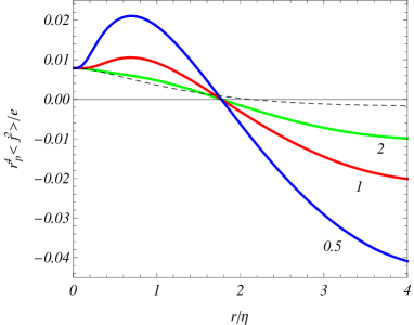
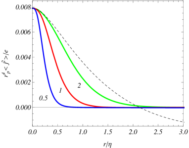
Figure 2: The azimuthal current density, multiplied by $r_{p}^{4}$, as a function of the distance from the $z$-axis for $\tilde{\beta}=0$ (left panel) and $\tilde{\beta}=1/2$ (right panel). The values of the other parameters are chosen as follows: $q=1$, $m\alpha=1$, $a_{0}=1/4$. The dashed curves correspond to the azimuthal current in the geometry of an uncompactified magnetic flux. The numbers near the curves correspond to the values of $L/\eta$.

In figure 3, the azimuthal current density is displayed as a function of $a_{0}$ (left panel) and $\tilde{\beta}$ (right panel) for different values of the parameter $q$ (numbers near the curves). The graphs are plotted for the values of the parameters $m\alpha=1$ and $L/\eta=r/\eta=1$. For the left panel we have taken $\tilde{\beta}=0$ and for the right one $a_{0}=1/4$.

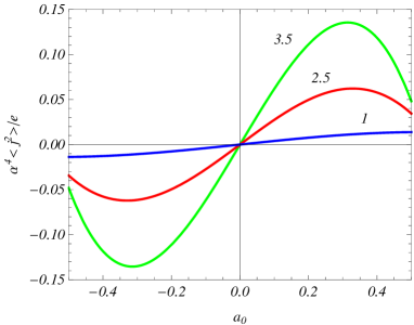
Figure 3: The azimuthal current density as a function of $a_{0}$ (left panel) and $\tilde{\beta}$ (right panel) for different values of the parameter $q$ (numbers near the curves). The graphs are plotted for $m\alpha=1$ and $L/\eta=r/\eta=1$. For the left panel $\tilde{\beta}=0$ and for the right one $a_{0}=1/4$.

4 Axial current

In this section we investigate the axial component of the current density. In order to do that we substitute the mode functions (2.24) and the relevant gamma matrices into (2.17) with $\mu=3$. After some intermediate steps the current density is presented in the form

$$\langle j^{3}\rangle = -\frac{eq\eta^{5}}{\pi^{2}L\alpha^{4}}\int_{0}^{\infty}dp\,p\,\sum_{j}[J_{\beta_{1}}^{2}(pr)+J_{\beta_{2}}^{2}(pr)]$$ (4.1)

$$\times\sum_{l=-\infty}^{+\infty}k_{l}\,\mathrm{Re\,}\left[K_{1/2+im\alpha}(i\gamma\eta)K_{1/2+im\alpha}(-i\gamma\eta)\right],$$

where we have replaced the Hankel functions by the MacDonald ones by using (3.4). To perform the summation over $l$, we use again the Abel-Plana formula (3.8) as we did for $\langle j^{2}\rangle$, taking $g(u)=u$ and the expression given in Eq. (3.9) for $f(u)$. The function $g(u)$ is an odd function which means that the first term on the rhs of the Abel-Plana formula vanishes. Therefore, the axial current in the geometry of a straight cosmic string vanishes. This result is in agreement with the one obtained for the flat space in the presence of the cosmic string [44].

The contribution to the axial current induced by the compactification is given by the second term in the rhs of the summation formula (3.8). It is written in the form

$$\langle j^{3}\rangle = -\frac{eq\eta^{5}i}{2\pi^{2}\alpha^{4}}\int_{0}^{\infty}dp\,p\,\sum_{j}[J_{\beta_{1}}^{2}(pr)+J_{\beta_{2}}^{2}(pr)]\int_{p}^{\infty}dk\,k\sum_{\chi=\pm 1}\frac{\chi}{e^{Lk+2\pi i\chi\tilde{\beta}}-1}$$ (4.2)

$$\times\mathrm{Re\,}\{K_{1/2+im\alpha}(\lambda\eta)\left[I_{-1/2-im\alpha}(\lambda\eta)+I_{1/2+im\alpha}(\lambda\eta)\right]\},$$

where $\lambda=\sqrt{k^{2}-p^{2}}$ and we have used the relation (3.32). For the further evaluation of this expression we first employ the expansion $\left(e^{u}-1\right)^{-1}=\sum_{l=1}^{\infty}e^{-lu}$ and then change to the new integration variable $\lambda$. This leads to the expression

$$\langle j^{3}\rangle = -\frac{eq\eta^{5}}{\pi^{2}\alpha^{4}}\sum_{l=1}^{\infty}\sin(2\pi\tilde{\beta}l)\int_{0}^{\infty}dp\,p\,\sum_{j}[J_{\beta_{1}}^{2}(pr)+J_{\beta_{2}}^{2}(pr)]\int_{0}^{\infty}d\lambda\,\lambda$$ (4.3)

$$\times e^{-lL\sqrt{\lambda^{2}+p^{2}}}\mathrm{Re\,}\{K_{1/2+im\alpha}(\lambda\eta)\left[I_{-1/2-im\alpha}(\lambda\eta)+I_{1/2+im\alpha}(\lambda\eta)\right]\}.$$

As the next step we use the integral representation

$$e^{-lL\sqrt{\lambda^{2}+p^{2}}}=\frac{lL}{\sqrt{\pi}}\int_{0}^{\infty}ds\,s^{-2}e^{-(\lambda^{2}+p^{2})s^{2}-l^{2}L^{2}/4s^{2}},$$ (4.4)

which is obtained from (3.34) by taking the derivative with respect to $L$. Substituting this identity into (4.3) and changing the order of integrations, the integrals over $\lambda$ and $p$ are evaluated with the help of formulas (3.35) and (3.36). Introducing the new integration variable $x=\eta^{2}/2s^{2}$, the final result is written as

$$\langle j^{3}\rangle = -\frac{\sqrt{2}eL}{\pi^{5/2}\alpha^{4}}\sum_{l=1}^{\infty}l\sin(2\pi\tilde{\beta}l)\int_{0}^{\infty}dx\,x^{3/2}\,e^{x\left(1-l^{2}L^{2}/2\eta^{2}\right)}$$ (4.5)

$$\times\mathrm{Re\,}\left[K_{1/2+im\alpha}(x)\right]\mathcal{F}(q,a_{0},xr^{2}/\eta^{2}),$$

with the function

$$\mathcal{F}(q,a_{0},z)=\frac{q}{2}e^{-z}\left[\mathcal{I}(q,a_{0},z)+\mathcal{I}(q,-a_{0},z)\right].$$ (4.6)

For the latter, by using the representation (3.18) for the function $\mathcal{I}(q,a_{0},z)$, one gets

$$\mathcal{F}(q,a_{0},z) = 1+2\sum_{k=1}^{p}(-1)^{k}\cos(2\pi ka_{0})\frac{\cos(\pi k/q)}{e^{2z\sin^{2}(\pi k/q)}}$$ (4.7)

$$+\frac{2q}{\pi}\int_{0}^{\infty}dx\frac{e^{-2z\cosh^{2}x}h(q,a_{0},2x)\sinh x}{\cosh(2qx)-\cos(q\pi)},$$

with the notation

$$h(q,a_{0},x)=\sum_{\chi=\pm 1}\cos\left[\left(1/2+\chi a_{0}\right)q\pi\right]\sinh\left[\left(1/2-\chi a_{0}\right)qx\right].$$ (4.8)

The axial current is an odd function of the parameter $\tilde{\beta}$ and an even function of $a_{0}$.

The part in the current density coming from the first term in the right-hand side of (4.7),

$$\langle j^{3}\rangle_{0}=-\frac{\sqrt{2}eL}{\pi^{5/2}\alpha^{4}}\sum_{l=1}^{\infty}l\sin(2\pi\tilde{\beta}l)\int_{0}^{\infty}dx\,x^{3/2}\,e^{x(1-l^{2}L^{2}/2\eta^{2})}\mathrm{Re\,}\left[K_{1/2+im\alpha}(x)\right],$$ (4.9)

does not depend on the planar angle deficit and magnetic flux along the string axis. It is a purely topological contribution and coincides with the current density in dS spacetime with spatial topology $R^{2}\times S^{1}$ in the absence of the string and of the magnetic flux along the $z$-axis. The fermionic current in $(D+1)$-dimensional dS spacetime with topology $R^{p}\times(S^{1})^{D-p}$ has been investigated in [47]. By using the integral representation

$$K_{\nu}(x)=2^{\nu-1}x^{-\nu}\int_{0}^{\infty}dy\,y^{\nu-1}e^{-y-x^{2}/4y},$$ (4.10)

and the formula (3.35), it can be seen that (4.9) coincides with the result from [47] in the special case $D=3$, $p=2$. The part in the axial current with the second and third terms on the right of (4.7) are induced by the presence of the string and of the magnetic flux along its axis.

In the absence of the cosmic string one has $q=1$ and from (4.5) we get

$$\langle j^{3}\rangle = \langle j^{3}\rangle_{0}-\frac{2\sqrt{2}eL\sin\left(a_{0}\pi\right)}{\pi^{7/2}\alpha^{4}}\sum_{l=1}^{\infty}l\sin(2\pi\tilde{\beta}l)\int_{0}^{\infty}du\,\sinh(2a_{0}u)$$ (4.11)

$$\times\tanh(u)\int_{0}^{\infty}dx\,x^{3/2}\,e^{x[1-2(r/\eta)^{2}\cosh^{2}u-l^{2}L^{2}/2\eta^{2}]}\mathrm{Re\,}\left[K_{1/2+im\alpha}(x)\right].$$

The second term on the rhs of this formula is induced by infinitely thin magnetic flux running along the compactified $z$-axis.

For a massless Dirac field the MacDonald function in the general formula (4.5) is expressed in terms of the exponential function. Substituting (4.7) into (4.5), after the integration over $z$ we find

$$\langle j^{3}\rangle = -\frac{4e(\eta/\alpha)^{4}}{\pi^{2}L^{3}}\sum_{l=1}^{\infty}l\sin(2\pi\tilde{\beta}l)\left[\frac{1}{l^{4}}+2\sum_{k=1}^{p}\frac{(-1)^{k}\cos(2\pi ka_{0})\cos(\pi k/q)}{[l^{2}+4(r/L)^{2}\sin^{2}(\pi k/q)]^{2}}\right.$$ (4.12)

$$\left.+\frac{2q}{\pi}\int_{0}^{\infty}dx\frac{h(q,a_{0},2x)\sinh x}{\cosh(2qx)-\cos(q\pi)}[l^{2}+4(r/L)^{2}\cosh^{2}x]^{-2}\right].$$

In this case the induced axial current is equal to $(\eta/\alpha)^{4}$ times the corresponding one in Minkowski spacetime in the presence of the cosmic string (the sign of the axial current obtained in [44] for the string in Minkowski bulk should be corrected to the opposite one).

Now let us consider the general formula (4.5) in various asymptotic regions of the parameters. At large distances from the string, $r/\eta\gg 1$, by taking into account that to the leading order $\mathcal{F}(q,a_{0},xr^{2}/\eta^{2})\approx 1$, we see that the current density coincides with the corresponding result in dS spacetime when the string and the magnetic flux along the $z$-axis are absent. In the region near the string, $r/\eta\ll 1$, we use the relation

$$\mathcal{F}(q,a_{0},z)\approx\frac{q(z/2)^{q(1/2-|a_{0}|)-1/2}}{2\Gamma(q(1/2-|a_{0}|)+1/2)},$$ (4.13)

for $z\ll 1$, which directly follows from (4.6). To the leading order this gives

$$\langle j^{3}\rangle = -\frac{eqL}{\sqrt{2}\pi^{5/2}\alpha^{4}}\frac{(r/\sqrt{2}\eta)^{q(1-2|a_{0}|)-1}}{\Gamma(q(1/2-|a_{0}|)+1/2)}\sum_{l=1}^{\infty}l\sin(2\pi\tilde{\beta}l)$$ (4.14)

$$\times\int_{0}^{\infty}dx\,x^{q(1/2-|a_{0}|)+1}\,e^{x\left(1-l^{2}L^{2}/2\eta^{2}\right)}\mathrm{Re\,}\left[K_{1/2+im\alpha}(x)\right].$$

The axial current vanishes on the string for $|a_{0}|<(1-1/q)/2$, is finite for $|a_{0}|=(1-1/q)/2$ and diverges for $|a_{0}|>(1-1/q)/2$. The irregular mode is responsible for the divergence in the latter case.

For small values of $L/\eta$, the dominant contribution to the axial current density comes from the part $\langle j^{3}\rangle_{0}$, corresponding to the current density in the geometry without the cosmic string and magnetic flux along the $z$-axis, and the contribution of the string-induced part is exponentially suppressed. By taking into account that in the limit under consideration the contribution of large $x$ dominates in the integral of (4.9), to the leading order we find

$$\langle j^{3}\rangle\approx-\frac{4\pi^{-2}e}{\left(\alpha/\eta\right)^{4}L^{3}}\sum_{l=1}^{\infty}\frac{\sin(2\pi\tilde{\beta}l)}{l^{3}}.$$ (4.15)

For large values $L/\eta$ with $r/\eta$ fixed, in the integral of (4.5) the contribution from the region near the lower limit dominates. By making use of (4.13), for the VEV of the axial current we get

$$\langle j^{3}\rangle \approx -\frac{2eqLB_{2}(m\alpha)(r/L)^{q(1-2|a_{0}|)-1}}{\pi^{5/2}(\alpha L/\eta)^{4}\Gamma(q(1/2-|a_{0}|)+1/2)}$$ (4.16)

$$\times\sum_{l=1}^{\infty}\frac{\sin(2\pi\tilde{\beta}l)}{l^{q(1-2|a_{0}|)+2}}\cos[2m\alpha\ln(lL/\eta)+\beta_{2}(m\alpha)],$$

where the functions $B_{2}(m\alpha)$ and $\beta_{2}(m\alpha)$ are defined by the relation (3.49). As is seen, for the length of the compact dimension larger than the curvature radius of dS spacetime the axial current decays as a power-law. For a string in background of Minkowski spacetime and for a massive fermionic field the axial current density decays as $e^{-mL}$.

In figure 4 the axial current density is displayed as a function of the ratio $r/\eta$ for $a_{0}=0$ (left panel) and $a_{0}=1/4$ (right panel). The numbers near the curves are the corresponding values of the parameter $q$. In both panels the graphs are plotted for $m\alpha=1$ and $\tilde{\beta}=1/4$. As it has been explained before, at large distances the axial current density tends to the limiting value corresponding to the geometry without the cosmic string and in the absence of the magnetic flux along the $z$-axis (the horizontal line in the left panel corresponding to $q=1$ and $a_{0}=0$).

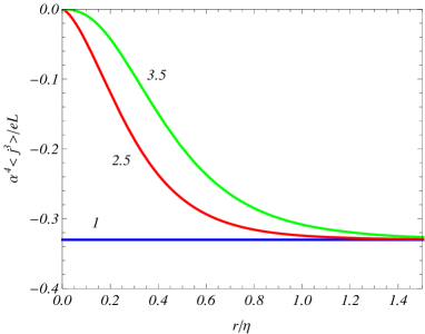
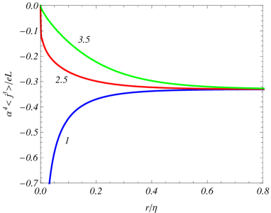
Figure 4: The axial current density as a function of $r/\eta$ for $a_{0}=0$ (left panel) and $a_{0}=1/4$ (right panel) and for separate values of $q$ (numbers near the curves). The graphs are plotted for $m\alpha=1$ and $\tilde{\beta}=1/4$.

The figure 5 presents the dependence of the axial current density on the parameters $a_{0}$ (left panel) and $\tilde{\beta}$ (right panel) for separate values of $q$ (numbers near the curves). For the left panel we have taken $\tilde{\beta}=1/4$ and for the right panel $a_{0}=0$. The values of the other parameters are as follows: $L/\eta=1$, $r/\eta=0.5$, $m\alpha=1$. Note that for fixed values of the other parameters the modulus of the axial current, $|\langle j^{3}\rangle|$, increases with increasing $q$ for $a_{0}$ close to $\pm 1/2$ and decreases for $a_{0}$ close to $0$.

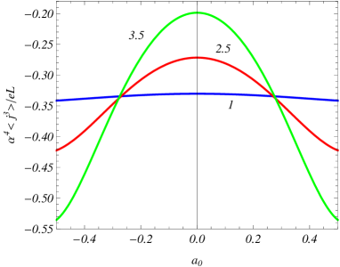
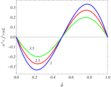
Figure 5: The axial current density versus $a_{0}$ (left panel) and $\tilde{\beta}$ (right panel) for different values of the parameter $q$ (the numbers near the curves). For the left panel $\tilde{\beta}=1/4$ and for the right one $a_{0}=0$. The graphs are plotted for $L/\eta=1$, $r/\eta=0.5$, $m\alpha=1$.

5 Conclusion

In this paper we have investigated the combined effects of the background gravitational field and topology on the VEV of the current density for a massive fermionic field. This quantity is an important local characteristic of the quantum vacuum. In addition to describing the physical structure of a charged quantum field at a given point, the VEV of the current density acts as the source in the semiclassical Maxwell equations and plays an important role in modeling a self-consistent dynamics involving the electromagnetic field. In order to have an exactly solvable problem, we have taken dS spacetime as the background geometry. The latter is among the most popular gravitational backgrounds and plays an important role in cosmology. The topological effects are induced by a cosmic string and by its compactification along the axis. Additionally, we have assumed the presence of a constant gauge field with nonzero axial and azimuthal components. By a gauge transformation, the problem is reduced to the one in the absence of a gauge field with the quasiperiodicity conditions (2.12) and (2.13) on the field operator. In the new representation, the information about the gauge field is encoded in the phases of these conditions.

For the evaluation of the VEV of the current density we have employed the direct summation over the complete set of fermionic modes. For the Bunch-Davies vacuum state, the corresponding mode functions are given by (2.24). For the model under consideration, in general, there is a one parameter family of boundary conditions imposed on the field operator at the location of the string. The fermionic modes used in the present paper correspond to the boundary condition when the MIT bag boundary condition is imposed at a finite radius, which is then taken to zero. The formal expression for the VEV of the induced fermionic current density is presented in the the mode-sum form (2.17). Because of the compactification of the cosmic string along its axis, the quantum number corresponding to the $z$-direction becomes discrete and for the corresponding summation we use the Abel-Plana-type formula (3.8). As a consequence, the current density is decomposed in two parts: the first part corresponds to the geometry of a straight cosmic string in dS spacetime and the second one is induced by the compactification. For a massless fermionic field, the problem under consideration is conformally related to the problem with a cosmic string in Minkowski spacetime and the corresponding expressions for the VEV of the current density are related by the standard conformal transformation.

In the problem under consideration the VEVs of the charge density and the radial current vanish. For the VEV of the azimuthal current density we have considered first the part corresponding to the geometry without compactification, denoted by $\langle j^{2}\rangle_{s}$. Two different integral representations for this part are provided, the expressions (3.16) and (3.26). The azimuthal current is an odd periodic function of the magnetic flux along the string axis with the period equal to the flux quantum. It depends on the radial and conformal time coordinates through the ratio $r/\eta$, which is the proper distance from the string measured in units of the dS curvature scale $\alpha$. Near the string, the leading term in the asymptotic expansion of $\langle j^{2}\rangle_{s}$ is independent of the mass and it behaves as the inverse forth power of the proper distance. In this limit the dominant contribution comes from the modes with small wavelengths and the effects of the curvature are small. For a massive field, the influence of the gravitational field on the vacuum current density is crucial at distances from the string larger than the curvature radius of the background spacetime. In this limit, corresponding to $r/\eta\gg 1$, the azimuthal current density exhibits a damping oscillatory behavior with the amplitude inversely proportional to the fourth power of the distance. Note that for the string in Minkowski spacetime and for a massive field, at large distances the current is exponentially suppressed.

The contribution to the azimuthal current density coming from the compactification of the string along its axis is given by (3.37) and the total current is given by (3.38). In the compactified geometry the azimuthal current is an odd periodic function of the magnetic flux along the string and an even periodic function of the flux enclosed by the $z$-axis. In both cases the period is equal to the flux quantum. Near the string the total azimuthal current is dominated by the part $\langle j^{2}\rangle_{s}$. In this region the leading term in the expansion of topological part is given by (3.42). This part vanishes on the string for $|a_{0}|<(1-1/q)/2$, is finite for $|a_{0}|=(1-1/q)/2$ and diverges for $|a_{0}|>(1-1/q)/2$. In the opposite limit of large distances from the string, the behavior of the azimuthal current density for a compactified cosmic string depends crucially on whether the parameter $\tilde{\beta}$, defined by (2.15), is zero or not. For $\tilde{\beta}\neq 0$ and $q>2$, the leading term in the asymptotic expansion is given by (3.44) and the azimuthal current is suppressed by the factor $e^{-4\pi\sigma_{\beta}r\sin(\pi/q)/L}$ with with $\sigma_{\beta}=\min(\tilde{\beta},1-\tilde{\beta})$. For $q\leqslant 2$ the suppression is stronger, by the factor $e^{-4\pi\sigma_{\beta}r/L}$. For $\tilde{\beta}=0$, at large distances the azimuthal current exhibits a damping oscillatory behavior described by (3.46). The amplitude of the oscillations decay as $(r/\eta)^{-3}$ and in this case the topological part $\langle j^{2}\rangle_{c}$ dominates in the total current density.

The VEV of the axial current density is given by the expression (4.5). The appearance of the nonzero axial current is a purely topological effect induced by the compactification of the string along its axis. The axial current density is an even periodic function of the magnetic flux along the string axis and an odd periodic function of the flux enclosed by the $z$-axis with the periods equal to the flux quantum. The modulus of the axial current, $|\langle j^{3}\rangle|$, increases with increasing $q$ for the values of the parameter $a_{0}$ close to $\pm 1/2$ and decreases for $a_{0}$ close to $0$. In the absence of the planar angle deficit one has $q=1$ and the general formula is reduced to (4.11). For general case of the parameter $q$, the corresponding asymptotic near the cosmic string is given by (4.14) and the axial current density vanishes on the string for $|a_{0}|<(1-1/q)/2$ and diverges for $|a_{0}|>(1-1/q)/2$. At large distances from the string the effects of the planar angle deficit and of the magnetic flux on the axial current are small and to the leading order we recover the result for dS spacetime with a single compact dimension, described by (4.9). For small values of the proper length of the compact dimension, the axial current is dominated by the part corresponding to the current density in the geometry without the cosmic string and magnetic flux along the $z$-axis. In this limit, the leding term in the asymptotic expansion is given by (4.15) and the string-induced corrections to this leading term are exponentially small. For large values of the ratio $L/\eta$, the behavior of the axial current is described by (4.16). In this range the current density exhibits damping oscillations with power-law decaying amplitude as a function of the length of the compact dimension. This behavior is essentially different from the case of the string in Minkowski bulk with the exponentially suppressed axial current for large values of $L$.

The results described above can be used, in particular, for the investigation of the effects induced by cosmic strings in the inflationary epoch. Though the strings produced before or during early stages of inflation are diluted by the expansion, cosmic strings can be continuously formed during inflation by coupling the symmetry breaking and inflaton fields [2] or by quantum-mechanical tunneling [62]. Another field of application corresponds to string-driven inflationary models with the cosmological expansion driven by the string energy [63].

References

- [1] N. D. Birrell and P. C.W. Davies, Quantum Fields in Curved Space (Cambridge University Press, Cambridge, 1982).
- [2] A. Vilenkin and E.P.S. Shellard, Cosmic Strings and Other Topological Defects (Cambridge University Press, Cambridge, England, 1994).
- [3] T. Damour and A. Vilenkin, Phys. Rev. Lett. 85, 3761 (2000); P. Battacharjee and G. Sigl, Phys. Rep. 327, 109 (2000); V. Berezinski, B. Hnatyk, and A. Vilenkin, Phys. Rev. D 64, 043004 (2001).
- [4] S. Sarangi and S.H.H. Tye, Phys. Lett. B 536, 185 (2002); E.J. Copeland, R.C. Myers, and J. Polchinski, JHEP 06, 013 (2004); G. Dvali and A. Vilenkin, JCAP 0403, 010 (2004); J. Polchinski, arXiv:hep-th/0410082.
- [5] T.M. Helliwell and D.A. Konkowski, Phys. Rev. D 34, 1918 (1986).
- [6] W.A. Hiscock, Phys. Lett. B 188, 317 (1987).
- [7] B. Linet, Phys. Rev. D 35, 536 (1987).
- [8] V.P. Frolov and E.M. Serebriany, Phys. Rev. D 35, 3779 (1987).
- [9] J.S. Dowker, Phys. Rev. D 36, 3095 (1987); J.S. Dowker, Phys. Rev. D 36, 3742 (1987).
- [10] A.G. Smith, in The Formation and Evolution of Cosmic Strings, Proceedings of the Cambridge Workshop, Cambridge, England, 1989, edited by G.W. Gibbons, S.W. Hawking, and T. Vachaspati (Cambridge University Press, Cambridge, England, 1990).
- [11] G.E.A. Matsas, Phys. Rev. D 41, 3846 (1990).
- [12] B. Allen and A.C. Ottewill, Phys. Rev. D 42, 2669 (1990); B. Allen, J.G. Mc Laughlin, and A.C. Ottewill, Phys. Rev. D 45, 4486 (1992).
- [13] T. Souradeep and V. Sahni, Phys. Rev. D 46, 1616 (1992).
- [14] K. Shiraishi and S. Hirenzaki, Class. Quantum Grav. 9, 2277 (1992).
- [15] V.B. Bezerra and E.R. Bezerra de Mello, Class. Quantum Grav. 11, 457 (1994); E.R. Bezerra de Mello, Class. Quantum Grav. 11, 1415 (1994).
- [16] D. Fursaev, Class. Quantum Grav. 11, 1431 (1994).
- [17] G. Cognola, K. Kirsten, and L. Vanzo, Phys. Rev. D 49, 1029 (1994).
- [18] M.E.X. Guimarães and B. Linet, Commun. Math. Phys. 165, 297 (1994).
- [19] B. Linet, J. Math. Phys. 36, 3694 (1995).
- [20] E.S. Moreira Jnr, Nucl. Phys. B 451, 365 (1995).
- [21] B. Allen, B.S. Kay, and A.C. Ottewill, Phys. Rev. D 53, 6829 (1996).
- [22] M. Bordag, K. Kirsten, and S. Dowker, Commun. Math. Phys. 182, 371 (1996).
- [23] D. Iellici, Class. Quantum Grav. 14, 3287 (1997).
- [24] N.R. Khusnutdinov and M. Bordag, Phys. Rev. D 59, 064017 (1999).
- [25] J. Spinelly and E.R. Bezerra de Mello, Class. Quantum Grav. 20, 873 (2003).
- [26] V.B. Bezerra and N.R. Khusnutdinov, Class. Quantum Grav. 23, 3449 (2006).
- [27] E.R. Bezerra de Mello, V.B. Bezerra, A.A. Saharian, and A.S. Tarloyan, Phys. Rev. D 74, 025017 (2006); E.R. Bezerra de Mello, V.B. Bezerraa, and A.A. Saharian, Phys. Lett. B 645, 245 (2007); E.R. Bezerra de Mello, V.B. Bezerra, A.A. Saharian, and A.S. Tarloyan, Phys. Rev. D 78, 105007 (2008).
- [28] M.E.X. Guimarães and B. Linet, Commun. Math. Phys. 165, 297 (1994).
- [29] J. Spinelly and E.R. Bezerra de Mello, Class. Quantum Grav. 20 874, (2003); J. Spinelly and E.R. Bezerra de Mello, Int. J. Mod. Phys. A, 17, 4375 (2002).
- [30] J. Spinelly and E.R. Bezerra de Mello, Int. J. Mod. Phys. D 13, 607 (2004); J. Spinelly and E.R. Bezerra de Mello, Nucl Phys. B (Proc. Suppl.) 127, 77 (2004).
- [31] J. Spinelly and E. R. Bezerra de Mello, JHEP 09, 005 (2008).
- [32] Yu.A. Sitenko and N.D. Vlasii, Class. Quantum Grav. 29, 095002 (2012).
- [33] L. Sriramkumar, Class. Quantum Grav. 18, 1015 (2001).
- [34] Yu.A. Sitenko and N.D. Vlasii, Class. Quantum Grav. 26, 195009 (2009).
- [35] E.R. Bezerra de Mello, Class. Quantum Grav. 27, 095017 (2010).
- [36] E.R. Bezerra de Mello, V.B. Bezerra, A.A. Saharian, and V.M. Bardeghyan, Phys. Rev. D 82, 085033 (2010).
- [37] P.C.W. Davies and V. Sahni, Class. Quantum Grav. 5, 1 (1988).
- [38] A.C. Ottewill and P. Taylor, Phys. Rev. D 82, 104013 (2010); A.C. Ottewill and P. Taylor, Class. Quantum Grav. 28, 015007 (2011).
- [39] E.R. Bezerra de Mello and A.A. Saharian, JHEP 04, 046 (2009).
- [40] E.R. Bezerra de Mello and A.A. Saharian, JHEP 08, 038 (2010).
- [41] E.R. Bezerra de Mello and A.A. Saharian, J. Phys. A: Math. Theor. 45 115402 (2012).
- [42] E.R. Bezerra de Mello and A.A. Saharian, Class. Quantum. Grav. 30 175001 (2013).
- [43] A.H. Castro Neto, F. Guinea, N.M.R. Peres, K.S. Novoselov, and A.K. Geim, Rev. Mod. Phys. 81, 109 (2009).
- [44] E. R. Bezerra de Mello and A. A. Saharian, Eur. Phys. J. C. 73, 2532 (2013).
- [45] S. Bellucci, E. R. Bezerra de Mello, A. de Padua, and A. A. Saharian, Eur. Phys. J. C. 74, 2688 (2014).
- [46] S. Bellucci, A.A. Saharian, and V.M. Bardeghyan, Phys. Rev. D 82, 065011 (2010); S. Bellucci and A.A. Saharian, Phys. Rev. D 87, 025005 (2013).
- [47] S. Bellucci, A.A. Saharian, and H.A. Nersisyan, Phys. Rev. D 88, 024028 (2013).
- [48] E.R. Bezerra de Mello and A.A. Saharian, Phys. Rev. D 87, 045015 (2013)
- [49] S. Bellucci, E.R. Bezerra de Mello, and A.A. Saharian, Phys. Rev. D 89, 085002 (2014).
- [50] A. M. Ghezelbash and R.B. Mann, Phys. Lett. B 537, 329 (2002).
- [51] J.D. Bjorken and S.D. Drell, Relativistic Quantum Mechanics (McGraw-Hill, New York, 1964).
- [52] T.S. Bunch and P.C.W. Davies, Proc. R. Soc. London A 360, 117 (1978).
- [53] P. de Sousa Gerbert and R. Jackiw, Commun. Math. Phys. 124, 229 (1989); P. de Sousa Gerbert, Phys. Rev. D 40, 1346 (1989); Yu.A. Sitenko, Ann. Phys. 282, 167 (2000).
- [54] C.G. Beneventano, M. De Francia, K. Kirsten, and E.M. Santangelo, Phys. Rev. D 61, 085019 (2000); M. De Francia and K. Kirsten, Phys. Rev. D 64, 065021 (2001).
- [55] S. Bellucci, E.R. Bezerra de Mello, and A.A. Saharian, Phys. Rev. D 83, 085017 (2011); E.R. Bezerra de Mello, F. Moraes, A.A. Saharian, Phys. Rev. D 85, 045016 (2012).
- [56] Yu.A. Sitenko, Phys. Rev. D 60, 125017 (1999).
- [57] M. Abramowitz and I.A. Stegun, Handbook of Mathematical Functions (National Bureau of Standards, Washington, DC, 1972).
- [58] A.A. Saharian, The Generalized Abel-Plana Formula with Applications to Bessel Functions and Casimir Effect (Yerevan State University Publishing House, Yerevan, 2008); Preprint ICTP/2007/082; arXiv:0708.1187.
- [59] E.R. Bezerra de Mello and A.A. Saharian, Phys. Rev. D 78, 045021 (2008); S. Bellucci and A.A. Saharian, Phys. Rev. D 79, 085019 (2009).
- [60] G.N. Watson, A Treatise on the Theory of Bessel Functions (Cambridge, Cambridge University Press, 1944).
- [61] I.S. Gradshteyn and I.M. Ryzhik, Table of Integrals, Series and Products (Academic Press, New York, 1980).
- [62] R. Basu, A.H. Guth, and A. Vilenkin, Phys. Rev. D 44, 340 (1991).
- [63] N. Turok, Phys. Rev. Lett. 60, 549 (1988).