Glauber gluons in spectator amplitudes for $B\to\pi M$ decays

Abstract

We extract the Glauber divergences from the spectator amplitudes for two-body hadronic decays $B\to M_{1}M_{2}$ in the $k_{T}$ factorization theorem, where $M_{2}$ denotes the meson emitted at the weak vertex. Employing the eikonal approximation, the divergences are factorized into the corresponding Glauber phase factors associated with the $M_{1}$ and $M_{2}$ mesons. It is observed that the latter factor enhances the spectator contribution to the color-suppressed tree amplitude by modifying the interference pattern between the two involved leading-order diagrams. The first factor rotates the enhanced spectator contribution by a phase, and changes its interference with other tree diagrams. The above Glauber effects are compared with the mechanism in elastic rescattering among various $M_{1}M_{2}$ final states, which has been widely investigated in the literature. We postulate that only the Glauber effect associated with a pion is significant, due to its special role as a $q\bar{q}$ bound state and as a pseudo Nambu-Goldstone boson simultaneously. Treating the Glauber phases as additional inputs in the perturbative QCD (PQCD) approach, we find a good fit to all the $B\to\pi\pi$, $\pi\rho$, $\pi\omega$, and $\pi K$ data, and resolve the long-standing $\pi\pi$ and $\pi K$ puzzles. The nontrivial success of this modified PQCD formalism is elaborated.

I INTRODUCTION

The known $B\to\pi\pi$ and $B\to\pi K$ puzzles have stimulated a lot of discussions in the literature: the measured $B^{0}\to\pi^{0}\pi^{0}$ branching ratio Amhis:2012bh is several times larger than the naive expectation, and the measured direct CP asymmetry in the $B^{\pm}\to\pi^{0}K^{\pm}$ decays dramatically differs from the $B^{0}\to\pi^{\mp}K^{\pm}$ one. It has been pointed out that these puzzles are sensitive to the least-understood color-suppressed tree amplitudes $C$ Charng2 ; Pham:2009ti ; CC09 . Other similar discrepancies were also observed: the $B^{0}\to\pi^{0}\rho^{0}$ branching ratios from the perturbative QCD (PQCD) and QCD factorization (QCDF) approaches, being sensitive to $C$, are lower than the data LY02 ; RXL ; BN . However, the estimate of $C$ from PQCD is well consistent with the measured $B^{0}\to\rho^{0}\rho^{0}$ branching ratio LM06 . Proposals resorting to new physics HLMN ; S08 ; FJPZ ; Baek:2008vr ; Bhattacharyya:2008vj ; Mohanta:2008ce ; Chang:2009wt ; Baek:2009hv ; Khalil:2009zf ; Huitu:2009st ; Cho:2011ta ; Imbeault:2008ge ; Endo:2012gi mainly resolved the $\pi K$ puzzle without addressing the peculiar feature of $C$ in the $\pi^{0}\pi^{0}$, $\pi^{0}\rho^{0}$, and $\rho^{0}\rho^{0}$ modes, while those to QCD effects are usually strongly constrained by the $\rho\rho$ data BRY06 . The recent resolution of the $B\to\pi K$ puzzle by means of the so-called Pauli blocking mechanism seems to be lack of a solid theoretical support Lipkin:2011ds . It manifests the difficulty of this subject.

Motivated by the above puzzles, we have carefully investigated the subleading contributions to the amplitudes $C$ and their impact on the $B\to\pi\pi$, $\pi K$ decays in the PQCD approach based on the $k_{T}$ factorization theorem KLS ; LUY . For example, the next-to-leading-order (NLO) contributions from the vertex corrections, the quark loops and the magnetic penguin have been calculated LMS05 ; X14 . Nevertheless, once a mechanism identified for $C$ respects the conventional factorization theorem, it is unlikely to be a resolution due to the $B\to\rho\rho$ constraint mentioned above LM06 . This is the reason why the above NLO corrections could not resolve the puzzles completely, though the consistency between the PQCD predictions and the data was improved. For a similar reason, higher-order corrections evaluated in QCDF BY05 , which obey the collinear factorization, cannot resolve the $B\to\pi\pi$ puzzle either. In a recent work LM11 , we have analyzed high-order corrections to the spectator diagrams in the $k_{T}$ factorization theorem, and found a new type of infrared divergences, called the Glauber gluons CQ06 . The all-order summation of the Glauber gluons leads to a phase factor, which modifies the interference between the spectator diagrams for $C$. We postulated that only the Glauber factors associated with a pion give significant effects, due to its special role as a $q\bar{q}$ bound state and as a pseudo Nambu-Goldstone (NG) boson simultaneously NS08 . It was then demonstrated that the Glauber effect, enhancing the magnitude of $C$, partially resolved the $B\to\pi\pi$ and $B\to\pi K$ puzzles. Our prediction for the $B^{0}\to\pi^{0}\pi^{0}$ branching ratio around $1.0\times 10^{-6}$ LM11 turns out to be consistent with the recent Belle data $(0.90\pm 0.12\pm 0.10)\times 10^{-6}$ update .

The above progress implies that the Glauber gluons in the $k_{T}$ factorization theorem deserve a thorough study. In this paper we shall examine whether the Glauber divergences in the spectator diagrams for the $B\to M_{1}M_{2}$ decay, where $M_{2}$ denotes the meson emitted at the weak vertex, have been extracted completely, and whether the same Glauber effect improves the consistency of the PQCD predictions with other data involving the pion, such as the $B\to\pi\rho,\pi\omega$ data. It will be shown that there exist the Glauber divergences associated with the $M_{1}$ meson, in additional to those associated with the $M_{2}$ meson LM11 . The all-order organization of the Glauber divergences follows the standard procedures, relying on the eikonal approximation for soft gluons. The resultant Glauber factor $\exp(-iS_{e1})$ from $M_{1}$ is the same for the two leading-order (LO) spectator diagrams. The Glauber factor from $M_{2}$ carries opposite phases, namely, $\exp(iS_{e2})$ for one diagram, and $\exp(-iS_{e2})$ for another. Therefore, they have different impacts on the amplitude $C$: the latter enhances the spectator contribution to $C$ by modifying the interference pattern between the two LO diagrams as mentioned before. The former rotates the enhanced spectator contribution by a phase, and changes its interference with other tree diagrams. The correspondence will be made explicit between the Glauber factors and the mechanism in elastic rescattering among various $M_{1}M_{2}$ final states, including the singlet exchange and the charge exchange, which have been widely explored in the literature CHY ; Chua08 .

The Glauber factors $\exp(-iS_{e1})$ (as $M_{1}=\pi$), and $\exp(\pm iS_{e2})$ (as $M_{2}=\pi$) are introduced into the PQCD factorization formulas for the spectator diagrams in the $B\to\pi\pi$, $\pi\rho$, $\pi\omega$, and $\pi K$ modes (totally 13 modes), and the phases $S_{e1}$ and $S_{e2}$ are treated as additional inputs. It turns out that the equal value $S_{e1}=S_{e2}\approx-\pi/2$ leads to a good fit to all the $B\to\pi M$ data. It will be observed that the Glauber effects render the NLO PQCD predictions for the $B^{0}\to\pi^{+}\pi^{-}$, $B^{+}\to\pi^{+}\pi^{0}$, and $B^{0}\to\pi^{0}\pi^{0}$ branching ratios agree well with the data. In particular, the rotation of the spectator amplitude by $\exp(-iS_{e1})$ is crucial for enhancing the ratio of the $B^{+}\to\pi^{+}\pi^{0}$ branching ratio over the $B^{0}\to\pi^{+}\pi^{-}$ one: this ratio depends on both the color-allowed tree amplitude $T$ and the color-suppressed tree amplitude $C$, so the relative phase between them matters. It is a nontrivial success that all the $B\to\pi\pi$, $\pi\rho$, and $\pi K$ puzzles mentioned before are resolved at the same time by introducing two Glauber phases.

In Sec. II we construct the standard meson wave functions for the $B\to M_{1}M_{2}$ decays in the $k_{T}$ factorization theorem, and analyze the residual infrared divergences caused by the Glauber gluons in the NLO spectator diagrams. The Glauber gluons associated with the $M_{1}$ and $M_{2}$ mesons are then factorized into the Glauber factors $\exp(-iS_{e1})$ and $\exp(\pm iS_{e2})$, respectively. In Sec. III we investigate the numerical impacts of the Glauber factors on the $B\to\pi\pi$, $\pi\rho$, $\pi\omega$, and $\pi K$ decays by presenting NLO PQCD predictions as contour plots in the $S_{e1}$-$S_{e2}$ plane. The agreement between the predictions and the data for the branching ratios and direct CP asymmetries as $S_{e1}=S_{e2}\approx-\pi/2$ is highlighted. Section IV contains the conclusion. The existence of the Glauber divergences is illustrated in the Appendix by means of the Feynman parametrization of loop integrands.

II FACTORIZATION OF GLAUBER GLUONS

It was pointed out CQ06 that the $k_{T}$ factorization theorem holds for simple processes like deeply inelastic scattering, but residual infrared divergences from the Glauber region may appear in complicated QCD processes like high-$p_{T}$ hadron hadroproduction. To factorize the collinear gluons associated with, say, one of the initial-state hadrons, one eikonalizes the particle lines to which the collinear gluons attach. Those eikonal lines from other hadrons should cancel in order to maintain the universality of the considered parton distribution function. However, the required cancellation is not exact in the $k_{T}$ factorization, leading to imaginary infrared logarithms, though it is in the collinear factorization. It has been demonstrated that the residual divergences can be factorized into a Glauber factor for low-$p_{T}$ hadron hadroproduction: the contour of a collinear gluon momentum can be deformed away from the Glauber region at low $p_{T}$, such that the usual eikonalization still holds CL09 . The above investigation was then extended to two-body hadronic $B$ meson decays $B\to M_{1}M_{2}$, and the residual infrared divergences in a spectator amplitude associated with the $M_{2}$ meson were found, and factorized into the same Glauber factor LM11 . Note that the $k_{T}$ factorization for a factorizable emission amplitude, i.e., a $B$ meson transition form factor, has been proved in NL03 .

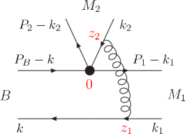
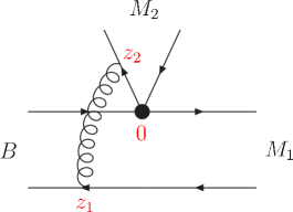
(a)	(b)

Figure 1: LO diagrams for a spectator amplitude.

In this section we shall perform a thorough study of the infrared divergences in the spectator diagrams at one-loop level of the $k_{T}$ factorization, following reasoning different from that in LM11 . Both the infrared divergences, which are absorbed into the standard meson wave functions, and the residual infrared divergences from the Glauber gluons associated with the mesons $M_{1}$ and $M_{2}$ will be extracted. Since we have postulated that only the Glauber effect from the pion is significant, it is not necessary to discuss the Glauber divergences associated with the $B$ meson. In principle, the Glauber gluons also exist in spectator penguin diagrams and in nonfactorizable annihilation diagrams, in which the hard gluon is emitted by the $b$ quark or by the spectator quark in the $B$ meson. As explained in LM11 , these diagrams are larger at LO, so they are more stable against subleading corrections. The Glauber effect is expected to be more significant in the spectator tree amplitudes, because of their tininess at LO.

Consider the $B(P_{B})\to M_{1}(P_{1})M_{2}(P_{2})$ decay, where $P_{B}$, $P_{1}$, and $P_{2}$ represent the momenta of the $B$, $M_{1}$, and $M_{2}$ mesons, respectively. For convenience, we choose $P_{B}=(P_{B}^{+},P_{B}^{-},{\bf 0}_{T})$ with $P_{B}^{+}=P_{B}^{-}=m_{B}/\sqrt{2}$, $m_{B}$ being the $B$ meson mass, and $P_{1}$ ($P_{2}$) in the plus (minus) direction. The parton four-momenta $k$, $k_{1}$, and $k_{2}$ are labelled in Fig. 1(a). After performing loop integrations, we keep $k^{-}=xP_{B}^{-}$, $k_{1}^{+}=x_{1}P_{1}^{+}$, $k_{2}^{-}=x_{2}P_{2}^{-}$, and transverse components $k_{T}$, that appear in the hard kernel for the $b$-quark decay. The order of magnitude $x_{2}\sim 0.5$, $x_{1}\sim 0.3$, $x\sim 0.1$, $m_{B}\sim 5$ GeV, and $k_{T}\lesssim 1$ GeV implies the hierarchy among the scales involved in exclusive $B$ meson decays in the small-$x$ region LSW12

$$m_{B}^{2},\,x_{2}m_{B}^{2}\gg x_{1}m_{B}^{2}\gg xm_{B}^{2}\gg xx_{1}m_{B}^{2},\,k_{T}^{2},$$ (1)

which will serve as a basis for higher-order analysis below.

We first identify the Glauber gluons associated with the LO spectator tree diagram in Fig. 1(a), originating from the operator $O_{2}$ REVIEW . Start with the set of NLO diagrams with a radiative gluon of momentum $l$ being emitted by the valence quark of $M_{2}$, as displayed in Fig. 2. Due to the soft cancellation between the gluons radiated by the valence quark and by the valence anti-quark of $M_{2}$ LT98 , only the collinear region with $l$ being collimated to $P_{2}$ is relevant here, and the $k_{T}$ dependence of parton propagators in the $B$ and $M_{1}$ mesons is negligible. The propagators of theses partons attached by the collinear gluons can then be approximated by the eikonal propagators $1/(l^{-}\pm i\epsilon)$. For a loop diagram to generate an imaginary Glauber logarithm, a necessary (but not sufficient) condition is that the interval of $l^{-}$ covers the origin $l^{-}=0$. The corresponding integral then contains an imaginary piece,

$${\rm Im}\int_{-a}^{b}dl^{-}\frac{1}{l^{-}+i\epsilon}=-\pi\int_{-a}^{b}dl^{-}\delta(l^{-})=-\pi,$$ (2)

under the principal-value prescription.

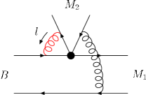
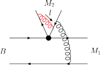
(a)	(b)	(c)
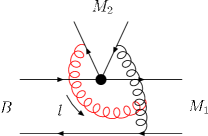
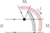
(d)	(e)	(f)

Figure 2: NLO diagrams for Fig. 1(a) that are relevant to the factorization of the $M_{2}$ meson wave function. Figures 2(d)-2(f) contribute to the Glauber divergences.

It has been shown that Figs. 2(a)-2(c) do not contain Glauber divergences, and contribute to the $M_{2}$ meson wave function LM11 . Take the vertex correction in Fig. 2(a) as an example. The integrand is proportional to

$$\frac{1}{2(P_{2}^{-}-k_{2}^{-}+l^{-})l^{+}-|{\bf k}_{2T}-{\bf l}_{T}|^{2}+i\epsilon}\frac{1}{2l^{-}l^{+}-l_{T}^{2}+i\epsilon}$$

$$\times\frac{1}{2(P_{B}^{-}-k^{-})l^{+}+2(P_{B}^{+}-k^{+}+l^{+})l^{-}+i\epsilon},$$ (3)

where $l$ denotes the loop momentum, and the transverse-momentum-dependent terms of the virtual $b$ quark propagator have been neglected in the heavy-quark limit. The contour integration over $l^{+}$ indicates that the loop integral does not vanish only for $l^{-}<0$: in this range there are poles located in the different half complex planes of $l^{+}$. Picking up the pole $l^{+}\approx 0-i\epsilon$ (see the power counting in Eq. (1)) associated with the valence quark propagator in $M_{2}$, namely, the first factor of Eq. (3), the $b$ quark propagator reduces to the eikonal propagator proportional to $1/(l^{-}+i\epsilon)$. In the range $l^{-}<0$ this propagator does not generate a Glauber divergence according to Eq. (2). Because it is factorized in color flow by itself with the color factor $C_{F}$, Fig. 2(a) leads to a Wilson line running from minus infinity to the origin, i.e, the weak vertex, which appears in the definition of the $M_{2}$ meson wave function. Similarly, the vertex correction in Fig. 2(b) is free of a Glauber divergence. Figure 2(c), with the collinear gluon attaching to the virtual quark line, does not produce an infrared Glauber divergence: the virtual quark line remains highly off-shell by $O(x_{1}m_{B}^{2})$ before and after the attachment of the collinear gluon according to Eq. (1), so no Glauber divergence is generated in this diagram.

As observed in LM11 , Figs. 2(d)-2(f) produce residual Glauber divergences under the hierarchical relation in Eq. (1), which demand introduction of an additional nonperturbative input. The integrand for Fig. 2(d) contains the five denominators

$$[(P_{2}-k_{2}+l)^{2}+i\epsilon][(k+l)^{2}+i\epsilon][(k-k_{1}+l)^{2}+i\epsilon](l^{2}+i\epsilon)[(k_{2}-k+k_{1}-l)^{2}+i\epsilon].$$ (4)

Non-vanishing contributions come from the ranges $0<l^{-}<k_{2}^{-}$, $-k^{-}<l^{-}<0$, and $-(P_{2}^{-}-k_{2}^{-})<l^{-}<-k^{-}$, where the poles of $l^{+}$ are given by

$$l^{+}\approx\frac{|{\bf l}_{T}-{\bf k}_{2T}|^{2}}{2(l^{-}+P_{2}^{-}-k_{2}^{-})}-i\epsilon(-i\epsilon,\;-i\epsilon),$$ (5)

$$l^{+}=-k^{+}+\frac{|{\bf l}_{T}+{\bf k}_{T}|^{2}}{2(l^{-}+k^{-})}-i\epsilon(-i\epsilon,\;+i\epsilon),$$ (6)

$$l^{+}=k_{1}^{+}+\frac{|{\bf l}_{T}-{\bf k}_{1T}+{\bf k}_{T}|^{2}}{2(l^{-}+k^{-})}-i\epsilon(-i\epsilon,\;+i\epsilon),$$ (7)

$$l^{+}=\frac{l_{T}^{2}}{2l^{-}}-i\epsilon(+i\epsilon,\;+i\epsilon),$$ (8)

$$l^{+}=k_{1}^{+}+\frac{|{\bf l}_{T}-{\bf k}_{2T}-{\bf k}_{1T}+{\bf k}_{T}|^{2}}{2(l^{-}-k_{2}^{-})}+i\epsilon(+i\epsilon,\;+i\epsilon),$$ (9)

respectively. We pick up the first pole $l^{+}\sim O(\Lambda_{\rm QCD}^{2}/m_{B})-i\epsilon$, which corresponds to the collinear gluon associated with the valence quark of $M_{2}$. It is seen that the allowed range for this pole, $-(P_{2}^{-}-k_{2}^{-})<l^{-}<k_{2}^{-}$, covers the origin $l^{-}=0$, leading to a Glauber divergence from the eikonalized spectator propagator $1/(k+l)^{2}$ and the on-shell radiative gluon. The other poles, such as those in Eqs. (6) and (7) in the range $-k^{-}<l^{-}<0$, should be included. However, it is easy to confirm that they are irrelevant to the analysis of the Glauber divergences. An alternative demonstration of the existence of the Glauber divergence in Fig. 2(d) by means of the Feynman parametrization of the corresponding loop integrand is presented in Appendix A.

For Fig. 2(e), the Ward identity is applied to the virtual gluon propagators,

$$\frac{1}{[(k-k_{1})^{2}+i\epsilon][(k-k_{1}+l)^{2}+i\epsilon]}=\left[\frac{1}{(k-k_{1})^{2}+i\epsilon}-\frac{1}{(k-k_{1}+l)^{2}+i\epsilon}\right]\frac{1}{l^{2}+2(k-k_{1})\cdot l+i\epsilon}.$$ (10)

Here we have chosen the sign of the $i\epsilon$ term in the factor outside the square brackets, such that this factor reduces to the eikonal propagator $1/(-l^{-}+i\epsilon)$, after picking up the pole $l^{+}\approx 0-i\epsilon$. With this choice the first term in the above splitting can be combined with Figs. 2(b) and 2(c), and contribute to the $M_{2}$ meson wave function with the piece of Wilson lines from a coordinate $z_{2}$ to plus infinity Li01 , where $z_{2}$ has been labelled in Fig. 1. As explicitly shown in Appendix A, the first term does not involve a Glauber divergence, so it does not break the universality of the $M_{2}$ meson wave function. The second piece in Eq. (10) with the color factor $N_{c}/2$, $N_{c}$ being the number of colors, contains the original Glauber divergence of Fig. 2(e). The eikonal approximation for the spectator propagator $1/[(k_{1}-l)^{2}+i\epsilon]$ in Fig. 2(f) also gives $1/(-l^{-}+i\epsilon)$ but with the color factor $-1/(2N_{c})$ LT98 . The sum of the second piece in Eq. (10) and Fig. 2(f) then leads to the Glauber divergence with the color factor $N_{c}/2-1/(2N_{c})=C_{F}$.

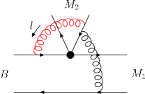
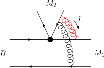
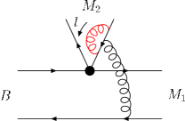
(a)	(b)	(c)
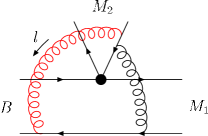
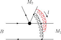
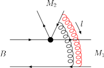
(d)	(e)	(f)

Figure 3: More NLO diagrams for Fig. 1(a).

We examine the effects from Fig. 3, which is similar to Fig. 2 but with the collinear gluon being emitted by the valence anti-quark of $M_{2}$. Figures 3(a)-3(c) do not generate Glauber divergences, and also contribute to the $M_{2}$ meson wave function. For example, the attachment to the $b$ quark in Fig. 3(a) gives rise to the eikonal propagator $1/(l^{-}+i\epsilon)$ as in Eq. (3), namely, the first piece of Wilson lines, which runs from minus infinity to the origin. Figure 3(d) contains the four denominators

$$[(k_{2}+l)^{2}+i\epsilon][(k+l)^{2}+i\epsilon][(k-k_{1}+l)^{2}+i\epsilon](l^{2}+i\epsilon),$$ (11)

whose corresponding $l^{+}$ poles are the same as in Eqs. (5)-(8). Therefore, the allowed range of $l^{-}$ reduces to $-(P_{2}^{-}-k_{2}^{-})<l^{-}<0$ without the pole in Eq. (9), and this diagram does not contain a Glauber divergence. This observation has been also confirmed in Appendix A by means of the Feynman parametrization of the corresponding loop integrand. Figures 2(d) and 3(d) have the same amplitudes in the soft region with $l\sim O(\Lambda_{\rm QCD})$ except a sign difference, which is attributed to the emissions of the collinear gluon by the valence quark and by the valence anti-quark in $M_{2}$. Because of this soft cancellation, the contour of $l^{-}$ in Fig. 2(d) can be deformed away the $O(\Lambda_{\rm QCD})$ region, and the eikonalization of the spectator $1/[(k+l)^{2}+i\epsilon]$ into $1/(l^{-}+i\epsilon)$ is justified LM11 . That is, Fig. 3(d) provides soft subtraction for Fig. 2(d), but does not remove its Glauber divergence. The soft cancellation also occurs between Figs. 2(e) and 3(e), and between Figs. 2(f) and 3(f).

The NLO residual infrared divergences in Figs. 2(d)-2(f) are then extracted from the Glauber region,

$$gC_{F}\int\frac{d^{4}l}{(2\pi)^{4}}tr\bigg{[}...\frac{-i(\not\!k_{2}-\not\!k+\not\!k_{1}-\not l)}{(k_{2}-k+k_{1}-l)^{2}+i\epsilon}(-ig\gamma_{\beta})\gamma_{5}\not\!\!P_{2}(-ig\gamma^{-})\frac{i(\not\!\!P_{2}-\not\!k_{2}+\not l)}{(P_{2}-k_{2}+l)^{2}+i\epsilon}\bigg{]}$$

$$\times\frac{-i}{(k-k_{1}+l)^{2}+i\epsilon}\frac{-i}{l^{2}+i\epsilon}2\pi i\delta(l^{-}),$$ (12)

where the $...$ denotes the rest of the integrand, and $\gamma_{5}\!\not\!\!P_{2}$ comes from the twist-2 structure of the $M_{2}$ meson wave function. The $l^{+}$ poles in Eq. (12) are given by Eqs. (5), (7), and (9) with $l^{-}=0$ from the valence quark propagator, the virtual gluon propagator, and the virtual quark propagator, respectively. Only the pole in Eq. (5) is of $O(\Lambda_{\rm QCD}^{2}/m_{B})$. As long as $k_{1}^{+}$ is of or greater than $O(\Lambda_{\rm QCD})$, we can deform the contour of $l^{+}$, such that $l^{+}$ remains $O(\Lambda_{\rm QCD})$, and the hierarchy

$$(P_{2}^{-}-k_{2}^{-})l^{+}\sim O(m_{B}\Lambda_{\rm QCD})\gg|{\bf l}_{T}-{\bf k}_{2T}|^{2}\sim O(\Lambda_{\rm QCD}^{2}),$$ (13)

holds. The valence quark carrying the momentum $P_{2}-k_{2}+l$ in Eq. (12) can then be eikonalized into $1/(l^{+}+i\epsilon)$.

Equation (12) is factorized into

$$g^{2}C_{F}\int\frac{d^{4}l}{(2\pi)^{4}}tr\bigg{[}...\frac{-i(\not\!k_{2}-\not\!k+\not\!k_{1}-\not l)}{(k_{2}-k+k_{1}-l)^{2}+i\epsilon}(-ig\gamma_{\beta})\gamma_{5}\not\!\!P_{2}\bigg{]}\frac{-i}{(k-k_{1}+l)^{2}+i\epsilon}$$

$$\times\frac{1}{l^{+}+i\epsilon}\frac{-i}{l^{2}+i\epsilon}2\pi i\delta(l^{-}).$$ (14)

The above factorization of the Glauber gluon follows exactly the reasoning applied to the low-$p_{T}$ hadron hadroproduction in CL09 . We close the contour in the lower half plane of $l^{+}$, and pick up only the pole $l^{+}\approx 0-i\epsilon$ from the eikonal propagator $1/(l^{+}+i\epsilon)$, which corresponds to an on-shell valence quark propagator. Another pole that corresponds to the on-shell right gluon contributes to the Glauber divergence associated with Fig. 1(b) LM11 . We then derive explicitly the imaginary logarithm,

$$i\frac{\alpha_{s}}{\pi}C_{F}\int\frac{d^{2}l_{T}}{l_{T}^{2}}{\cal M}_{a}^{(0)}({\bf l}_{T}),$$ (15)

where ${\cal M}_{a}^{(0)}$ denotes the LO spectator amplitude from Fig. 1(a). The gluon propagator proportional to $1/l_{T}^{2}$ indicates that the infrared divergence we have identified arises from the Glauber region.

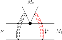
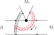
(a)	(b)	(c)

Figure 4: NLO diagrams for Fig. 1(b) that contribute to the Glauber divergences associated with the $M_{2}$ meson.

Below we investigate the Glauber divergences appearing in the NLO corrections to Fig. 1(b), which are associated with the $M_{2}$ meson. The relevant diagrams contain the attachments of the collinear gluons emitted by the valence anti-quark of $M_{2}$ as depicted in Fig. 4. For the attachment to the virtual gluon in Fig. 4(b), we adopt the splitting

$$\frac{1}{[(k-k_{1})^{2}+i\epsilon][(k-k_{1}+l)^{2}+i\epsilon]}=\left[\frac{1}{(k-k_{1})^{2}+i\epsilon}-\frac{1}{(k-k_{1}+l)^{2}+i\epsilon}\right]\frac{1}{l^{2}+2(k-k_{1})\cdot l-i\epsilon},$$ (16)

where the second term on the right-hand side contains the Glauber divergence in the original NLO diagram. The first term then contributes to the definition of the $M_{2}$ meson wave function. The similar analysis implies that the diagrams in Fig. 4 contain the Glauber divergences,

$$-i\frac{\alpha_{s}}{\pi}C_{F}\int\frac{d^{2}l_{T}}{l_{T}^{2}}{\cal M}_{b}^{(0)}({\bf l}_{T}),$$ (17)

where ${\cal M}_{b}^{(0)}$ denotes the LO spectator amplitude from Fig. 1(b). The additional minus sign compared to Eq. (15) is attributed to the collinear gluon emission by the valence anti-quark of $M_{2}$.

(a)	(b)
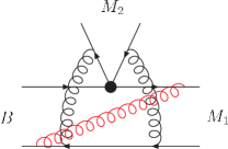
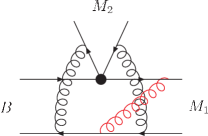
(c)	(d)

Figure 5: (a)-(c) Higher-order corrections to Fig. 1 that contain the Glauber divergences associated with the $M_{1}$ meson. (d) Higher-order correction to Fig. 1 that does not contain the Glauber divergence associated with the $M_{1}$ meson.

It has been shown that the residual infrared divergences appear between the $M_{2}$ meson and the $B\to M_{1}$ transition LM11 . It is natural to ask whether there exist more residual infrared divergences in the spectator amplitude of the $B\to M_{1}M_{2}$ decay. We shall verify that it is the case: additional Glauber divergences associated with the $M_{1}$ meson are induced by the inclusion of the Glauber divergences associated with the $M_{2}$ meson. Consider all possible attachments of the collinear gluons emitted by the valence quark of $M_{1}$ to particle lines in Fig. 1(a), among which the diagram in Fig. 5(a) contains a Glauber divergence as implied by the pole analysis of the following five denominators

$$[(P_{1}-k_{1}+l)^{2}+i\epsilon][(k+l)^{2}+i\epsilon][(k-k_{1}+l)^{2}+i\epsilon](l^{2}+i\epsilon)[(k_{2}-k+k_{1}-l)^{2}+i\epsilon].$$ (18)

Non-vanishing contributions come from the ranges $0<l^{+}<k_{1}^{+}$, $-k^{+}<l^{+}<0$, and $-(P_{1}^{+}-k_{1}^{+})<l^{+}<-k^{+}$, where the poles of $l^{-}$ are given by

$$l^{-}\approx\frac{|{\bf l}_{T}-{\bf k}_{1T}|^{2}}{2(l^{+}+P_{1}^{+}-k_{1}^{+})}-i\epsilon(-i\epsilon,\;-i\epsilon),$$ (19)

$$l^{-}=-k^{-}+\frac{|{\bf l}_{T}+{\bf k}_{T}|^{2}}{2(l^{+}+k^{+})}-i\epsilon(-i\epsilon,\;+i\epsilon),$$ (20)

$$l^{-}=\frac{l_{T}^{2}}{2l^{+}}-i\epsilon(+i\epsilon,\;+i\epsilon),$$ (21)

$$l^{-}=-k^{-}+\frac{|{\bf l}_{T}-{\bf k}_{1T}+{\bf k}_{T}|^{2}}{2(l^{+}-k_{1}^{+})}+i\epsilon(+i\epsilon,\;+i\epsilon),$$ (22)

$$l^{-}=k_{2}^{-}+\frac{|{\bf l}_{T}-{\bf k}_{2T}-{\bf k}_{1T}+{\bf k}_{T}|^{2}}{2(l^{+}-k_{1}^{+})}+i\epsilon(+i\epsilon,\;+i\epsilon),$$ (23)

respectively. We pick up the first pole $l^{-}\sim O(\Lambda_{\rm QCD}^{2}/m_{B})-i\epsilon$, which corresponds to the collinear gluon associated with the valence quark of $M_{1}$. It is seen that the allowed range for this pole, $-(P_{1}^{+}-k_{1}^{+})<l^{+}<k_{1}^{+}$, covers the origin $l^{+}=0$, leading to a Glauber divergence from the eikonalized spectator propagator $1/(k+l)^{2}$ and the on-shell radiative gluon.

The residual Glauber divergence in Fig. 5(a) yields the NLO spectator amplitude

$$g\frac{-1}{2N_{c}}\int\frac{d^{4}l}{(2\pi)^{4}}tr\bigg{[}...(-ig\gamma^{+})\frac{i(\not\!P_{1}-\not\!k_{1}+\not l)}{(P_{1}-k_{1}+l)^{2}+i\epsilon}\gamma_{\mu}(1-\gamma_{5})\frac{-i(\not\!k_{2}-\not\!k+\not\!k_{1}-\not l)}{(k_{2}-k+k_{1}-l)^{2}+i\epsilon}(-ig\gamma_{\beta})\gamma_{5}\not\!\!P_{2}\bigg{]}$$

$$\times\frac{-i}{(k-k_{1}+l)^{2}+i\epsilon}\frac{-i}{l^{2}+i\epsilon}\pi i\delta(l^{+}).$$ (24)

The $l^{-}$ poles in the above expression are given by Eqs. (19) and (23) with $l^{+}=0$ from the valence quark propagator in $M_{1}$ and the virtual quark propagator, respectively. The pole in Eq. (19) is of $O(\Lambda_{\rm QCD}^{2}/m_{B})$, and the pole in Eq. (23) is of $O(m_{B})$, so we can deform the contour of $l^{-}$, such that $l^{-}$ remains at least $O(\Lambda_{\rm QCD})$, and the hierarchy

$$(P_{1}^{+}-k_{1}^{+})l^{-}\sim O(m_{B}\Lambda_{\rm QCD})\gg|{\bf l}_{T}-{\bf k}_{1T}|^{2}\sim O(\Lambda_{\rm QCD}^{2}),$$ (25)

holds. The valence quark carrying the momentum $P_{1}-k_{1}+l$ is thus eikonalized into $1/(l^{-}+i\epsilon)$. Equation (24) is factorized into

$$g^{2}\frac{-1}{2N_{c}}\int\frac{d^{4}l}{(2\pi)^{4}}tr\bigg{[}...\gamma_{\mu}(1-\gamma_{5})\frac{-i(\not\!k_{2}-\not\!k+\not\!k_{1}-\not l)}{(k_{2}-k+k_{1}-l)^{2}+i\epsilon}(-ig\gamma_{\beta})\gamma_{5}\not\!\!P_{2}\bigg{]}\frac{-i}{(k-k_{1}+l)^{2}+i\epsilon}$$ (26)

$$\times\frac{1}{l^{-}+i\epsilon}\frac{-i}{l^{2}+i\epsilon}\pi i\delta(l^{+}),$$

$$\approx -i\frac{1}{2N_{c}}\frac{\alpha_{s}}{2\pi}\int\frac{d^{2}l_{T}}{l_{T}^{2}}{\cal M}_{a}^{(0)}({\bf l}_{T}),$$

where we have closed the contour in the lower half plane of $l^{-}$ over the pole $l^{-}\approx 0-i\epsilon$ from the eikonal propagator $1/(l^{-}+i\epsilon)$.

Figure 5(b) gives the Glauber divergence the same as in Eq. (26), since the collinear gluon is also emitted by the valence quark of $M_{1}$ and attaches to the spectator of the $B$ meson:

$$-i\frac{1}{2N_{c}}\frac{\alpha_{s}}{2\pi}\int\frac{d^{2}l_{T}}{l_{T}^{2}}{\cal M}_{b}^{(0)}({\bf l}_{T}).$$ (27)

The Glauber divergences in Eqs. (26) and (27) can also be verified by means of the Feynman parametrization of the loop integrands, as shown in Appendix A. Because of the destruction between the LO amplitudes ${\cal M}_{a}^{(0)}$ and ${\cal M}_{b}^{(0)}$, these Glauber divergences cancel each other. The same cancellation also occurs between the pair of diagrams with the collinear gluons attaching to the virtual gluons in Figs. 1(a) and 1(b). It then implies that there is no more Glauber divergence at NLO in the $B\to M_{1}M_{2}$ decay, except those associated with the $M_{2}$ meson. The other collinear gluon emissions from the valence quark and from the spectator of $M_{1}$ contribute only to the construction of the $M_{1}$ meson wave function, which contains the Wilson lines running from the origin to infinity, and then from the infinity to the coordinate $z_{1}$ labelled in Fig. 1(a). The cancellation of the soft divergences, similar to that between Figs. 2 and 3, also occurs between the above two sets of diagrams.

Nevertheless, the Glauber divergences associated with the $M_{1}$ meson exist at next-to-next-to-leading order. Once the Glauber gluons associated with the $M_{2}$ meson are included, the interference between the two spectator amplitudes ${\cal M}_{a}$ and ${\cal M}_{b}$ becomes constructive, and the cancellation between Eqs. (26) and (27) does not take place anymore. A corresponding diagram is displayed in Fig. 5(c), in which the two vertical gluon lines contribute to the Glauber divergences for Figs. 1(a) and 1(b), and the third gluon emitted by $M_{1}$ gives a common Glauber divergence. The color factor for Fig. 5(c) is given by

$$tr\left(T^{c}T^{a}T^{b}T^{c}T^{b}T^{a}\right)=\frac{1}{2}tr(T^{a}T^{b})tr(T^{b}T^{a})-\frac{1}{2N_{c}}tr\left(T^{a}T^{b}T^{b}T^{a}\right),$$ (28)

where $T^{a}$, $T^{b}$, and $T^{c}$ are associated with the left vertical gluon, the right vertical gluon, and the third gluon, respectively. The first term in the above expression corresponds to a color flow from the four-fermion operator $O_{1}$. Since we focus on the spectator amplitude from $O_{2}$ in this work, this contribution will be dropped. The second term corresponds to the color flow of the original spectator amplitude, implying that the color factors for the Glauber divergences associated with the $M_{2}$ and $M_{1}$ mesons remain as in Eqs. (15), (17), (26), and (27).

It can be shown that the attachments of the third gluon to other lines, for example, to the spectator line between the two vertical gluons in Fig. 5(d), do not produce Glauber divergences. The reason is explained below. We route the loop momentum of the third gluon through the left-handed vertical gluon. When this left-handed vertical gluon is hard (the right-handed vertical gluon is soft), the third gluon contributes only to the $M_{1}$ meson wave function: the diagram can be regarded as a two-particle reducible correction to the $M_{1}$ meson wave function with the right-handed vertical soft gluon coupling the $M_{2}$ meson and the $B$-$M_{1}$ system. That is, it does not contribute to the Glauber divergence, which breaks the factorization. When the left-handed vertical gluon is soft (the right-handed vertical gluon is hard), the valence quark of the $M_{2}$ meson remains on-shell and collimated to the $M_{2}$ meson. In this case its momentum is independent of $k_{1}$, and it does not constrain the contour in the $l^{-}$ plane. When both vertical gluons are hard, Fig. 5(d) contributes to the NLO hard kernel, which goes beyond the accuracy of the present calculation.

A remark is in order. It has been shown that the Glauber divergence exists in Fig. 2(f), where the radiative gluon of momentum $l$ attaches partons in the $M_{1}$ and $M_{2}$ mesons. A simple way to tell whether this Glauber divergence is associate with the $M_{1}$ or $M_{2}$ meson is to investigate the pole structures. Replacing the spectator propagator by $\delta(l^{-})$ as done in Eq. (12), we check the pole positions in the complex $l^{+}$ plane, and find that the $l^{+}$ contour for Fig. 2(f) is constrained by the valence quark propagator and the valence anti-quark propagator of $M_{2}$. On the contrary, replacing the valence quark propagator of $M_{2}$ by $\delta(l^{+})$, we see that the $l^{-}$ contour is not constrained. The above different pole structures between $l^{+}$ and $l^{-}$ implies that the observed Glauber divergence should be associated with the $M_{2}$ meson. We then complete the investigation of the Glauber divergences in the spectator amplitudes for the two-body hadronic $B$ meson decays. The exponentiation of the NLO results in Eqs. (15) and (17) LM11 , and in Eqs. (26) and (27) leads to the parametrization

$$M_{a}^{G} = \exp(-iS_{e1})\exp(iS_{e2}){\cal M}_{a}^{(0)},$$

$$M_{b}^{G} = \exp(-iS_{e1})\exp(-iS_{e2}){\cal M}_{b}^{(0)},$$ (29)

where the signs have followed the indication of the NLO results. It is obvious that the destruction between $M_{a}^{G}$ and $M_{b}^{G}$ retains, as the Glauber factors associated with the $M_{2}$ meson are turned off, i.e., $S_{e2}=0$. Strictly speaking, Eq. (29), derived with the dependence on the Glauber gluon transverse momentum being neglected, holds only approximately. We shall treat the Glauber phases $S_{e1}$ and $S_{e2}$ as free parameters in the numerical analysis later. A definition for the Glauber factor in terms of a matrix element of four Wilson lines has been constructed in CL09 .

At last, we point out the connection between the Glauber gluon exchanges and the elastic scattering in two-body hadronic $B$ meson decays. The analysis of CHY ; Chua08 started with the amplitudes evaluated in the QCDF approach, and final-state interaction effects were included via the elastic rescattering. Take the rescattering only between the $B^{0}\to\pi^{+}\pi^{-}$ and $B^{0}\to\pi^{0}\pi^{0}$ modes as an example,

$$\left(\begin{array}[]{c}\pi^{+}\pi^{-}\\ \pi^{0}\pi^{0}\end{array}\right)=S^{1/2}_{\rm res}\left(\begin{array}[]{c}\pi^{+}\pi^{-}\\ \pi^{0}\pi^{0}\end{array}\right)_{\rm QCDF},$$ (30)

with the matrix $S^{1/2}_{\rm res}\equiv(1+i{\cal T})^{1/2}$ parameterizing the rescattering effects. The matrix $\cal T$ is written as

$$\cal T=\left(\begin{array}[]{cc}r_{0}+2r_{a}+r_{t}&(2r_{a}-r_{e}+r_{t})/\sqrt{2}\\ (2r_{a}-r_{e}+r_{t})/\sqrt{2}&r_{0}+(2r_{a}+r_{e}+r_{t})/2\end{array}\right),$$ (33)

where the parameters $r_{0}$, $r_{e}$ $r_{a}$, and $r_{t}$ denote the mechanism from the singlet exchange, the charge exchange, the annihilation, and the total annihilation, respectively. The best fit to the $B\to PP$ data gave the following combined parameters defined in Eq. (15) of Chua08

$$1+i(r_{0}+r_{a})=0.94+0.58\,i,\;\;\;\;i(r_{e}-r_{a})=0.06-0.58\,i,\;\;\;\;i(r_{a}+r_{t})=-0.12-0.09\,i,$$ (34)

which seem to indicate that the annihilation and the total annihilation are less important, and $r_{0}$ and $r_{e}$ are roughly of the same order of magnitude.

Compared to the above formalism, the standard NLO PQCD decay amplitudes correspond to the inputs on the right-hand side of Eq. (30), and the Glauber gluon exchanges correspond to the matrix $\cal T$. The Glauber gluons do not generate the annihilation $r_{a}$ and $r_{t}$, an observation consistent with the numerical outcomes in Eq. (34). We elaborate that the amplitude in Eq. (15) contributes to $r_{0}$, and that in Eq. (17) contributes to $r_{e}$. Insert the identity for the color matrices

$$I_{ij}I_{lk}=\frac{1}{N_{c}}I_{lj}I_{ik}+2(T^{c})_{lj}(T^{c})_{ik},$$ (35)

into $M_{b}^{G}$, with $I_{ij}$ ($I_{lk}$) being the unity matrix associated with the meson $M_{1}$ ($M_{2}$). The second term in the decomposition, associated with a meson in the color-octet state, will not be considered here. The matrix $I_{lj}$ in the first term implies that the valence quark in $M_{1}$ and the valence anti-quark in $M_{2}$ form a color-singlet state. The matrix $I_{ik}$ implies that the valence anti-quark in $M_{1}$ and the valence quark in $M_{2}$ form a color-singlet state. It is easy to see that the resultant topology corresponds to the color-allowed tree amplitude $T$. Therefore, $M_{b}^{G}$ can be regarded as a contribution from the $B^{0}\to\pi^{+}\pi^{-}$ intermediate state, dominated by the amplitude $T$, to the $B^{0}\to\pi^{0}\pi^{0}$ decay, dominated by $C$, through the mechanism of charge exchange. The above color rearrangement does not apply to the amplitude $M_{a}^{G}$, since the color trace of $I_{lj}$ and the color matrix associated with the hard gluon vertex vanishes. Hence, $M_{a}^{G}$ represents the contribution from the $B^{0}\to\pi^{0}\pi^{0}$ intermediate state to itself through the singlet exchange. Certainly, the Glauber effect and the elastic rescattering are essentially different. For instance, the former is crucial only in the pion-involved decays, while the latter contributes to all relevant modes under the $SU(3)$ flavor symmetry.

III NUMERICAL ANALYSIS

As postulated in LM11 , the Glauber effect from the multi-parton states is more significant in the pion than in other mesons. This postulation can be understood by means of the simultaneous role of the pion as a $q\bar{q}$ bound state and as a NG boson NS08 : the valence quark and anti-quark of the pion are separated by a short distance in order to reduce the confinement potential energy, while the multi-parton states of the pion spread over a huge space-time in order to meet the role of a massless NG boson. That is, the multi-parton states distribute more widely than the $q\bar{q}$ state does in the pion compared to other mesons. This explains the strong Glauber effect from the pion, which will be examined in this section. The standard PQCD factorization formulas for the $B\to\pi\pi$ and $\pi K$ decays are referred to LMS05 , while those for the $B\to\pi\rho$ and $\pi\omega$ decays LY02 ; RXL can be obtained by taking into account the differences between $B\to PP$ and $PV$ modes as illustrated in LM062 .

Following Eq. (29), we multiply the $b$-quark spectator amplitudes in NLO PQCD, both tree and penguin, by $\exp(iS_{e2})$ ($\exp(-iS_{e2})$) with the hard gluon being emitted by the valence anti-quark (quark) in $M_{2}$, if $M_{2}$ denotes a pion. We also multiply the above spectator amplitudes by $\exp(-iS_{e1})$, if $M_{1}$ denotes a pion. As mentioned in LMS05 , the color-suppressed tree amplitude in the $B\to\pi\pi$ decays is small at LO due to the small Wilson coefficient $a_{2}$ for the factorizable contribution and to the cancellation between Figs. 1(a) and 1(b) for the spectator contribution. The presence of the Glauber factor $\exp(\pm iS_{e2})$ converts the destructive interference in Fig. 1 into a constructive one, resulting in strong enhancement. The Glauber factor $\exp(-iS_{e1})$ further rotates the enhanced spectator amplitude, and modifies its interference with other emission amplitudes. This effect will adjust the relative phase between the color-allowed and color-suppressed tree amplitudes, such that all the three $B\to\pi\pi$ branching ratios are accommodated at the same time.

The choices of the distribution amplitudes for the $B$ meson, pseudo-scalar mesons and vector mesons are the same as in LM062 , but with the updated values of the meson decay constants: $f_{B}=191$ MeV, $f_{\pi}=130$ MeV, $f_{K}=156$ MeV, $f_{\rho}=216$ MeV, $f_{\rho}^{T}=165$ MeV, $f_{\omega}=187$ MeV, and $f_{\omega}^{T}=151$ MeV PDG ; Ball06 . We also update the meson masses $m_{B}=5.28$ GeV, $m_{\pi}=0.137$ GeV, $m_{K}=0.495$ GeV, $m_{\rho}=0.77$ GeV, and $m_{\omega}=0.783$ GeV, the quark masses $m_{q}=6.5$ MeV, $m_{s}=140$ MeV, $m_{c}=1.5$ GeV, and $m_{b}=4.8$ GeV, which appear in the quark-loop and magnetic-penguin amplitudes, the chiral scales $m_{0\pi}=1.6$ GeV and $m_{0K}=1.8$ GeV, the $B$ meson lifetimes $\tau_{B^{0}}=1.519\times 10^{-12}$ sec and $\tau_{B^{\pm}}=1.641\times 10^{-12}$ sec, and the CKM matrix elements $V_{ud}=0.97427$, $V_{us}=0.22534$, $|V_{ub}|=3.51\times 10^{-3}$, $V_{cd}=-0.22520$, $V_{cs}=0.97344$, and $V_{cb}=0.0412$, and the weak phases $\phi_{1}=21.5^{\circ}$ and $\phi_{3}=70^{\circ}$ Amhis:2012bh ; PDG , while the other parameters are taken to be the same as in LM062 . We employ the NLO Wilson coefficients for the emission amplitudes, and the LO ones for the the annihilation amplitudes, since the NLO corrections to the weak vertices in the latter are not yet available. The resultant $B\to\pi,K,\rho,\omega$ transition form factors are then given by

$$F_{0}^{B\pi}(0)=0.28,\ \ \ \ \ \ F_{0}^{BK}(0)=0.39,\ \ \ \ \ \ A_{0}^{B\rho}(0)=0.29,\ \ \ \ \ \ A_{0}^{B\omega}(0)=0.27,$$ (36)

at maximal recoil, close to those obtained in KLS02 .

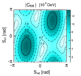
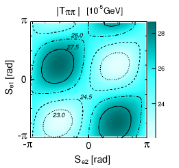
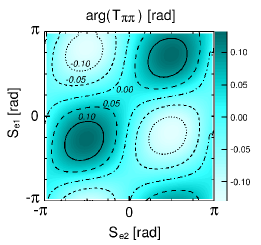
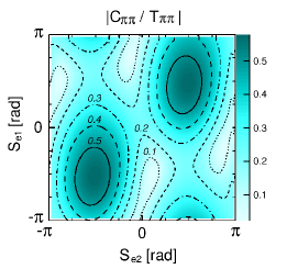
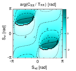
Figure 6: $S_{e1}$ and $S_{e2}$ dependencies of the amplitudes $C$ and $T$, and their ratio $C/T$ for the $B\to\pi\pi$ decays.

The $S_{e1}$ and $S_{e2}$ dependencies of the color-suppressed tree amplitude $C$, the color-allowed tree amplitude $T$, and their ratio for the $B\to\pi\pi$ decays are displayed in Fig. 6, where the definitions of $C$ and $T$ are the same as in LMS05 . As argued before, the destructive interference between Figs. 1(a) and 1(b) is moderated by the Glauber factor, so their net contribution increases for nonvanishing $S_{e2}$. It is observed in Fig. 6 that the magnitude of $C$ reaches maximum as $S_{e2}\approx-\pi/2$. On the other hand, Figs. 1(a) and 1(b) acquire the same phase factor $\exp(-iS_{e1})$ from the Glauber gluons in the $M_{1}$ meson. Despite of being an overall factor, it changes the relative phase between the spectator amplitude and the factorizable emission amplitude, which includes the important vertex corrections at NLO LMS05 . Therefore, $C$ also depends on $S_{e1}$, whose magnitude reaches maximum for $S_{e1}\approx S_{e2}\approx-\pi/2$. Because $T$ receives contributions from both the factorizable and spectator diagrams, the Glauber factors affect its magnitude and argument. Due to the dominance of the former contribution, the Glauber effect is minor on $T$, compared to that on $C$. Figure 6 exhibits that the magnitude of the amplitude ratio $C/T$ is enhanced by factor 3 as $S_{e1}\approx S_{e2}\approx-\pi/2$, relative to the value at $S_{e1}=S_{e2}=0$. The result $C/T=0.58e^{-0.9i}$ at $S_{e1}=S_{e2}=-\pi/2$ for the $B\to\pi\pi$ decays is close to the extraction in Charng2 .

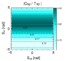
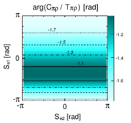
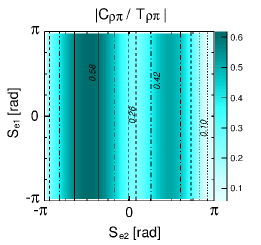
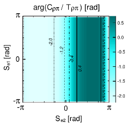
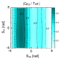
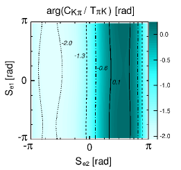
Figure 7: $S_{e1}$ and $S_{e2}$ dependencies of the amplitudes $C$ and $T$, and their ratio $C/T$ for the $B\to\pi\rho$ and $\pi K$ decays.

Similar plots for the $B\to\pi\rho$ and $\pi K$ decays are displayed in Fig. 7. The plots for the $B\to\pi\omega$ decays, similar to those for the $B\to\pi\rho$ ones, are not presented here. Since only a single pion is involved in each mode, either the Glauber phase $S_{e1}$ or $S_{e2}$ appears in the modified PQCD factorization formula. For those modes containing the $B\to\pi$ transition, the corresponding amplitude ratio $C_{\pi\rho}/T_{\pi\rho}$ depends on $S_{e1}$ only: the magnitude of $C_{\pi\rho}/T_{\pi\rho}$ decreases by about 40%, and the argument decreases by about 10% as $S_{e1}$ varies from zero to $-\pi/2$. For those modes with $M_{2}=\pi$, the corresponding amplitude ratios $C_{\rho\pi}/T_{\rho\pi}$ and $C_{K\pi}/T_{\pi K}$ mainly depend on $S_{e2}$: both the magnitude and argument increase by a factor 2, as $S_{e2}$ varies from zero to $-\pi/2$. As explained before, the variation of $S_{e2}$ modifies the interference pattern between the two spectator diagrams in Fig. 1, such that the corresponding Glauber effect always enhances the magnitude of $C/T$. Compared to the $B\to\pi\pi$ case, the Glauber effects are minor in the $B\to\pi\rho$, $\pi\omega$, and $\pi K$ decays as expected.

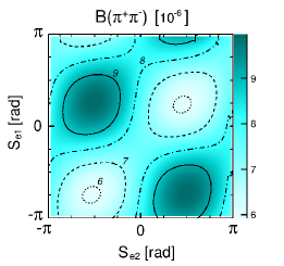
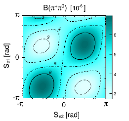
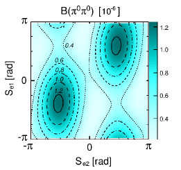
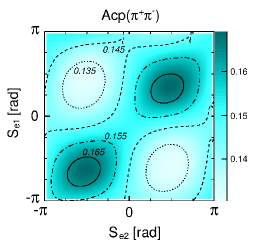
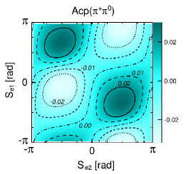
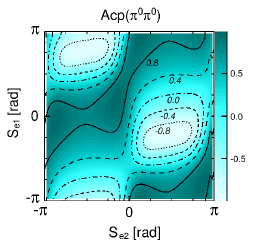
Figure 8: $S_{e1}$ and $S_{e2}$ dependencies of the $B\to\pi\pi$ branching ratios (in units of $10^{-6}$) and direct CP asymmetries.

The $S_{e1}$ and $S_{e2}$ dependencies of the $B\to\pi\pi$ branching ratios (in units of $10^{-6}$) and direct CP asymmetries are shown in Fig. 8. It is found that the combined effect from the two Glauber factors decreases the $B^{0}\to\pi^{+}\pi^{-}$ branching ratio from $7.5\times 10^{-6}$ (corresponding to $S_{e1}=S_{e2}=0$) to $6.4\times 10^{-6}$ (corresponding to $S_{e1}=S_{e2}=-\pi/2$). On the contrary, the $B^{+}\to\pi^{+}\pi^{0}$ branching ratio increases from $5.0\times 10^{-6}$ to $6.6\times 10^{-6}$. That is, the ratio of the above two predictions becomes consistent with the data. The Glauber effect is not dramatic, because these two modes are dominated by the color-allowed tree amplitude $T$. The enhancement of the $B^{0}\to\pi^{0}\pi^{0}$ branching ratio from about $0.38\times 10^{-6}$ to $1.2\times 10^{-6}$ is significant, rendering the NLO PQCD prediction agree well with the data $(1.17\pm 0.13)\times 10^{-6}$. Note that the above data have been updated by combining the BaBar ones in Amhis:2012bh with those recently reported by Belle update . The improved consistency of the three predicted branching ratios with the data is highly nontrivial, which requires the simultaneous adjustment of the relative phases between the spectator diagrams, and between the spectator amplitude and other emission amplitudes. It is seen that the Glauber factor does not change much the direct CP asymmetries in the $B^{0}\to\pi^{+}\pi^{-}$ and $B^{+}\to\pi^{+}\pi^{0}$ decays, which contain the amplitude $T$. The impact on the $B^{0}\to\pi^{0}\pi^{0}$ direct CP asymmetry is obvious in Fig. 6: the predicted $A_{CP}(\pi^{0}\pi^{0})$ decreases from 0.59 to 0.36, closer to the central value of the data $0.03\pm 0.17$, when one varies the phases from $S_{e1}=S_{e2}=0$ to $S_{e1}=S_{e2}=-\pi/2$. The above data have been also updated by combining the BaBar ones in Amhis:2012bh with those recently reported by Belle update .

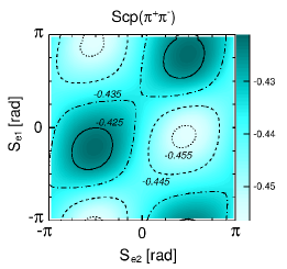
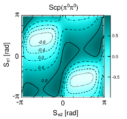
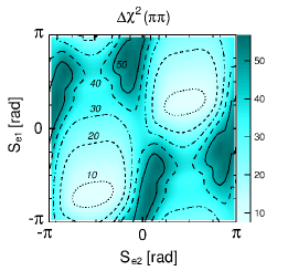
Figure 9: $S_{e1}$ and $S_{e2}$ dependencies of the $B\to\pi\pi$ mixing-induced CP asymmetries, and $\Delta\chi^{2}$.

The NLO PQCD predictions for the mixing-induced CP asymmetries in the $B\to\pi\pi$ decays with the variation of $S_{e1}$ and $S_{e2}$ are exhibited in Fig. 9. The prediction for $S_{CP}(\pi^{0}\pi^{0})$ is more sensitive to the Glauber phases compared to that for $S_{CP}(\pi^{+}\pi^{-})$, since the $B^{0}\to\pi^{+}\pi^{-}$ mode is dominated by the color-allowed tree amplitude. The latter remains around $-0.43$ under the variation of $S_{e1}$ and $S_{e2}$, which is lower than the data $-0.66\pm 0.06$ Amhis:2012bh . The former reduces from $0.80$ to $0.63$, as one tunes the phases from $S_{e1}=S_{e2}=0$ to $S_{e1}=S_{e2}=-\pi/2$. To quantize the improvement of the consistency between the PQCD predictions and the data attributed to the inclusion of the Glauber phases, we define

$$\Delta\chi^{2}=\frac{({\rm data}\;{\rm mean}-{\rm theory}\;{\rm value})^{2}}{\sqrt{{\rm data\;error}^{2}+(0.30\times{\rm theoty\;value})^{2}}},$$ (37)

where the unknown theoretical uncertainty is assumed to be 30%. We stress that we have not attempted to undertake the best fit, but illustrate the improvement by computing $\Delta\chi^{2}$. The last plot in Fig. 9 summarizes the reduction of $\Delta\chi^{2}$ in the global fit of the PQCD predictions with the Glauber phases to the $B\to\pi\pi$ data. As expected, the value drops significantly from about 36 (corresponding to $S_{e1}=S_{e2}=0$) to around 11 (corresponding to $S_{e1}=S_{e2}=-\pi/2$). That is, the Glauber gluons indeed affect the ratio $C/T$ toward the indication of the data.

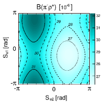
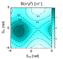
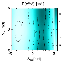
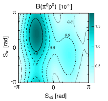
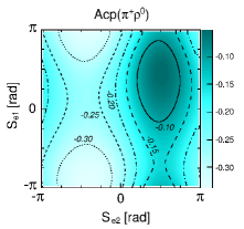
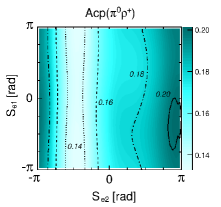
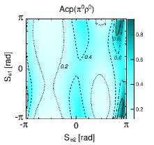
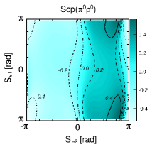
Figure 10: $S_{e1}$ and $S_{e2}$ dependencies of the $B\to\pi\rho$ branching ratios (in units of $10^{-6}$), direct CP asymmetries, and mixing-induced CP asymmetry.

The $S_{e1}$ and $S_{e2}$ dependencies of the $B\to\pi\rho$ branching ratios (in units of $10^{-6}$) and direct CP asymmetries are shown in Fig. 10. Because only a single pion is involved in these modes, the Glauber effect is minor. The NLO PQCD prediction for the branching ratio $B(\pi^{\pm}\rho^{\mp})$ increases a bit from $27.8\times 10^{-6}$ to $30.8\times 10^{-6}$, as one tunes the phases from $S_{e1}=S_{e2}=0$ to $S_{e1}=S_{e2}=-\pi/2$, which slightly overshoots the data. The predicted $B(\pi^{+}\rho^{0})$ increases from $6.5\times 10^{-6}$ to $7.2\times 10^{-6}$, while the predicted $B(\pi^{0}\rho^{+})$ decreases from $13.3\times 10^{-6}$ to $9.3\times 10^{-6}$. The predicted $B(\pi^{0}\rho^{0})$ changes more dramatically under the variation of the Glauber factors, since it is dominated by the color-suppressed tree amplitude: it is enhanced from $0.70\times 10^{-6}$ to about $1.1\times 10^{-6}$. The predictions for $B(\pi^{+}\rho^{0})$ and $B(\pi^{0}\rho^{0})$ become closer to the data. The current data for the direct CP asymmetries in the $B\to\pi\rho$ decays and for the mixing-induced CP asymmetry $S_{CP}(\pi^{0}\rho^{0})$ still suffer huge uncertainties.

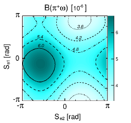
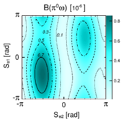
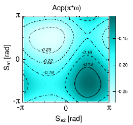
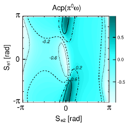
Figure 11: $S_{e1}$ and $S_{e2}$ dependencies of the $B\to\pi\omega$ branching ratios (in units of $10^{-6}$), direct CP asymmetries, and mixing-induced CP asymmetry.

The behavior of the $B\to\pi\omega$ modes with the Glauber phases is similar to that of the corresponding $B\to\pi\rho$ modes, as shown in Fig. 11. The NLO PQCD prediction for $B(\pi^{+}\omega)$ increases from $5.4\times 10^{-6}$ to $6.1\times 10^{-6}$, as one tunes the phases from $S_{e1}=S_{e2}=0$ to $S_{e1}=S_{e2}=-\pi/2$. The modified result is more consistent with the data $(6.9\pm 0.5)\times 10^{-6}$ Amhis:2012bh . The prediction for $B(\pi^{0}\omega)$ increases from $0.04\times 10^{-6}$ to $0.85\times 10^{-6}$, above the upper bound $0.5\times 10^{-6}$ Amhis:2012bh . As remarked before, the present formalism is a simplified one with the convolution between the Glauber factors and the standard PQCD factorization formulas being neglected. We shall refine our predictions, when the data for $B(\pi^{0}\omega)$ become available. As to the direct CP asymmetries, the predicted $A_{CP}(\pi^{+}\omega)$ remains around $-0.2$ under the variation of the Glauber phases. The CP asymmetries $A_{CP}(\pi^{0}\omega)$ and $S_{CP}(\pi^{0}\omega)$ are more sensitive to the Glauber phases, and the predicted value for the former (latter) varies from $-0.99$ to $-0.12$ (from $-0.11$ to $-0.26$). The current data for the direct CP asymmetries and mixing-induced CP asymmetry either have large uncertainties, or are not yet available.

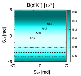
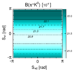
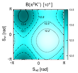
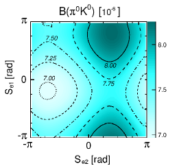
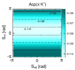
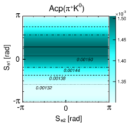
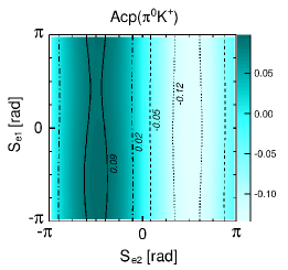
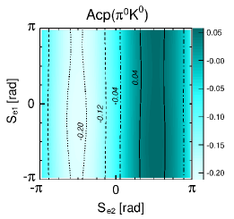
Figure 12: $S_{e1}$ and $S_{e2}$ dependencies of the $B\to\pi K$ branching ratios (in units of $10^{-6}$), direct CP asymmetries, and mixing-induced CP asymmetry.

The $S_{e1}$ and $S_{e2}$ dependencies of the $B\to\pi K$ branching ratios (in units of $10^{-6}$), direct CP asymmetries, and mixing-induced CP asymmetry are displayed in Fig. 12. It is easy to understand that the PQCD predictions for all the branching ratios depend on the Glauber phases weakly. $B(\pi^{-}K^{+})$ and $B(\pi^{+}K^{0})$ are insensitive to the variation of $S_{e2}$, since these two modes do not involve the color-suppressed tree amplitude. The weak dependence on $S_{e1}$ is introduced through the interference between the spectator diagrams and the factorizable emission diagrams. $B(\pi^{0}K^{+})$ and $B(\pi^{0}K^{0})$ depend on both Glauber phases, because of the involvement of the color-suppressed tree amplitude. For a similar reason, the direct CP asymmetries $A_{CP}(\pi^{-}K^{+})$ and $A_{CP}(\pi^{+}K^{0})$ are insensitive to the variation of $S_{e2}$, and slightly depend on $S_{e1}$. The prediction for $A_{CP}(\pi^{-}K^{+})$ remains as $-0.11$, as varying $S_{e1}$, close to the data $-0.082\pm 0.006$ Amhis:2012bh . On the contrary, $A_{CP}(\pi^{0}K^{+})$ and $A_{CP}(\pi^{0}K^{0})$ depend on $S_{e2}$, but are not sensitive to $S_{e1}$. Note that the amplitude $C$ contains the $B\to K$ transition in this case, and the Glauber effect from the kaon is assumed to be negligible. The predicted $A_{CP}(\pi^{0}K^{+})$ increases from $-0.01$, and becomes positive quickly, as $S_{e2}$ approaches $-\pi/2$, a tendency in agreement with the updated data $0.040\pm 0.021$ Amhis:2012bh . The prediction for $A_{CP}(\pi^{0}K^{0})$ decreases from $-0.08$ to $-0.21$. This difference is attributed to the sign flip of $C$ between the above two modes. Figure 12 indicates that the mixing-induced CP asymmetry $S_{CP}(\pi^{0}K^{0})$ descends from $0.75$ to $0.69$. Compared to the data $S_{CP}(\pi^{0}K^{0})=0.57\pm 0.17$ and $S_{CP}(c\bar{c}s)=0.682\pm 0.019$ Amhis:2012bh , the consistency has been improved.

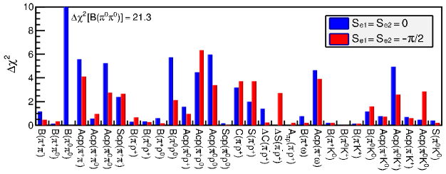
Figure 13: $S_{e1}$ and $S_{e2}$ dependencies of $\Delta\chi^{2}$ for all the $B\to\pi\pi$, $\pi\rho$, $\pi\omega$, and $\pi K$ decays. The difference of $\Delta\chi^{2}$ for each considered quantity due to the inclusion of the Glauber effects is also displayed.

At last, we display the $S_{e1}$ and $S_{e2}$ dependencies of $\Delta\chi^{2}$ for the fit to all the $B\to\pi\pi$, $\pi\rho$, $\pi\omega$, and $\pi K$ data in Fig. 13, which exhibits significant decrease of $\Delta\chi^{2}$ from 76 to 49, as both $S_{e1}$ and $S_{e2}$ change from zero to $-\pi/2$. Figure 13 also shows the change of $\Delta\chi^{2}$ for each mode caused by $S_{e1}=S_{e2}=-\pi/2$. The major reduction of $\Delta\chi^{2}$ arises from the modified predictions for the $B\to\pi\pi$ decays, especially from the $B^{0}\to\pi^{0}\pi^{0}$ branching ratio. The amount of reduction of $\Delta\chi^{2}$ from the $B\to\pi\rho$, $\pi\omega$, and $\pi K$ modes is minor. To summarize the Glauber effects on the quantities considered above, we present the branching ratios and direct CP asymmetries from the data, the standard NLO PQCD predictions with $S_{e}=S_{e1}=S_{e2}=0$, and the modified predictions with $S_{e}=-\pi/2$ in Table 1. Those for the mixing-induced CP asymmetries are listed in Table 2. At last, we compute the CP violation parameters $C$, $\Delta C$, $S$, $\Delta S$, and $A_{\pi\rho}$ associated with the $B^{0}\to\pi^{\mp}\rho^{\mp}$ decays, which are defined in Amhis:2012bh , and present the results in Table 3. Our predictions for these observables can be confronted with future data.

	Data Amhis:2012bh ; update	$S_{e}=0$	$S_{e}=-\pi/2$		Data Amhis:2012bh ; update	$S_{e}=0$	$S_{e}=-\pi/2$
$B(B^{0}\to\pi^{\mp}\pi^{\pm})$	$5.10\pm 0.19$	$7.5$	$6.4$	$A_{CP}(B^{0}\to\pi^{\mp}\pi^{\pm})$	$0.31\pm 0.05$	$0.15$	$0.17$
$B(B^{\pm}\to\pi^{\pm}\pi^{0})$	$5.48^{+0.35}_{-0.34}$	$5.0$	$6.6$	$A_{CP}(B^{\pm}\to\pi^{\pm}\pi^{0})$	$0.026\pm 0.039$	$-0.003$	$-0.012$
$B(B^{0}\to\pi^{0}\pi^{0})$	$1.17\pm 0.13$	$0.38$	$1.2$	$A_{CP}(B^{0}\to\pi^{0}\pi^{0})$	$0.03\pm 0.17$	$0.59$	$0.36$
$B(B^{0}\to\pi^{\mp}\rho^{\pm})$	$23.0\pm 2.3$	$27.8$	$30.8$
$B(B^{\pm}\to\pi^{0}\rho^{\pm})$	$10.9^{+1.4}_{-1.5}$	$13.3$	$9.3$	$A_{CP}(B^{\pm}\to\pi^{0}\rho^{\pm})$	$0.02\pm 0.11$	$0.17$	$0.13$
$B(B^{\pm}\to\pi^{\pm}\rho^{0})$	$8.3^{+1.2}_{-1.3}$	$6.5$	$7.2$	$A_{CP}(B^{\pm}\to\pi^{\pm}\rho^{0})$	$0.18^{+0.09}_{-0.17}$	$-0.20$	$-0.31$
$B(B^{0}\to\pi^{0}\rho^{0})$	$2.0\pm 0.5$	$0.70$	$1.1$	$A_{CP}(B^{0}\to\pi^{0}\rho^{0})$	$-0.27\pm 0.24$	$0.38$	$0.18$
$B(B^{\pm}\to\pi^{\pm}\omega)$	$6.9\pm 0.5$	$5.4$	$6.1$	$A_{CP}(B^{\pm}\to\pi^{\pm}\omega)$	$-0.02\pm 0.06$	$-0.20$	$-0.18$
$B(B^{0}\to\pi^{0}\omega)$	$<0.5$	$0.04$	$0.85$	$A_{CP}(B^{0}\to\pi^{0}\omega)$	—–	$-0.99$	$-0.12$
$B(B^{\pm}\to\pi^{\pm}K^{0})$	$23.79\pm 0.75$	$20.9$	$21.1$	$A_{CP}(B^{\pm}\to\pi^{\pm}K^{0})$	$-0.015\pm 0.019$	$0.001$	$0.001$
$B(B^{\pm}\to\pi^{0}K^{\pm})$	$12.94^{+0.52}_{-0.51}$	$12.2$	$12.9$	$A_{CP}(B^{\pm}\to\pi^{0}K^{\pm})$	$0.040\pm 0.021$	$-0.01$	$0.10$
$B(B^{0}\to\pi^{\mp}K^{\pm})$	$19.57^{+0.53}_{-0.52}$	$17.6$	$17.7$	$A_{CP}(B^{0}\to\pi^{\mp}K^{\pm})$	$-0.082\pm 0.006$	$-0.11$	$-0.11$
$B(B^{0}\to\pi^{0}K^{0})$	$9.93\pm 0.49$	$7.5$	$7.2$	$A_{CP}(B^{0}\to\pi^{0}K^{0})$	$-0.01\pm 0.10$	$-0.08$	$-0.21$

Table 1: Branching ratios (in units of $10^{-6}$) and direct CP asymmetries, with the notation $S_{e}\equiv S_{e1}=S_{e2}$.

	Data Amhis:2012bh	$S_{e}=0$	$S_{e}=-\pi/2$		Data Amhis:2012bh	$S_{e}=0$	$S_{e}=-\pi/2$
$S_{CP}(B^{0}\to\pi^{\mp}\pi^{\pm})$	$-0.66\pm 0.06$	$-0.44$	$-0.43$	$S_{CP}(B^{0}\to\pi^{0}\pi^{0})$	—–	$0.80$	$0.63$
$S_{CP}(B^{0}\to\pi^{0}\rho^{0})$	$-0.23\pm 0.34$	$-0.09$	$-0.30$	$S_{CP}(B^{0}\to\pi^{0}\omega)$	—–	$-0.11$	$-0.26$
$S_{CP}(B^{0}\to\pi^{0}K^{0})$	$0.57\pm 0.17$	$0.75$	$0.69$

Table 2: Mixing-induced CP asymmetries.

	Data Amhis:2012bh	$S_{e}=0$	$S_{e}=-\pi/2$		Data Amhis:2012bh	$S_{e}=0$	$S_{e}=-\pi/2$
$C$	$-0.03\pm 0.06$	$0.09$	$0.10$	$\Delta C$	$0.27\pm 0.06$	$0.44$	$0.32$
$S$	$0.06\pm 0.07$	$-0.04$	$-0.08$	$\Delta S$	$0.01\pm 0.08$	$0.004$	$-0.14$
${\cal A}_{\pi\rho}$	$-0.11\pm 0.03$	$-0.11$	$-0.13$

Table 3: CP violation parameters for the $B^{0}\to\pi^{\mp}\rho^{\mp}$ decays.

IV CONCLUSION

In this paper we have identified the uncancelled Glauber divergences in the $k_{T}$ factorization theorem for the spectator amplitudes in the $B\to M_{1}M_{2}$ decays at NLO level. It has been shown that the divergences are factorizable and demand the introduction of the phase factors: those coupling the $M_{1}$ meson and the $B$-$M_{2}$ system are absorbed into the phase factor $\exp(-iS_{e1})$, and those coupling the $M_{2}$ meson and the $B\to M_{1}$ transition are absorbed into $\exp(\pm iS_{e2})$. We have investigated the Glauber effects on the color-suppressed tree amplitude $C$ and the color-allowed tree amplitude $T$ in a simplified formalism, in which the convolution between the Glauber factors and the standard PQCD factorization formulas is neglected. Treating $S_{e1}$ and $S_{e2}$ as free parameters, it was observed that the ratio $C/T$ is enhanced maximally by a factor 3, and a good fit of the PQCD predictions to all the considered $B\to\pi\pi$, $\pi\rho$, $\pi\omega$, and $\pi K$ data is achieved as $S_{e1}=S_{e2}\approx-\pi/2$.

We summarize the modified NLO PQCD predictions: $B(\pi^{0}\pi^{0})$ and $B(\pi^{0}\rho^{0})$ are increased, the difference between $A_{CP}(\pi^{\mp}K^{\pm})$ and $A_{CP}(\pi^{0}K^{\pm})$ is enlarged, and $\Delta S_{\pi^{0}K_{S}}$ is reduced, all becoming more consistent with the data. The major reduction of $\Delta\chi^{2}$ in the global fit arises from the observables for the $B\to\pi\pi$ modes. We stress again that the above improvement is nontrivial, since the simultaneous adjustment of the phases between the spectator diagrams, and between the spectator amplitude and other emission amplitudes for these modes is required. The constraint on $C$ from the $B\to\rho\rho$ data is evaded, because of the special role of the pion as a $q\bar{q}$ bound state and as a pseudo NG boson. It seems that the implication on new physics from the $B\to\pi K$ puzzle tends to be weaker Ciuchini:2008eh ; Baek:2009pa .

The Glauber gluons may have the nonperturbative origin similar to that in elastic rescattering. The correspondence has been made explicit between the Glauber factors and the mechanism in elastic rescattering among various $M_{1}M_{2}$ final states, including the singlet exchange and the charge exchange CHY ; Chua08 . A derivation of the Glauber factor, or even an evaluation of the parameters $S_{e1}$ and $S_{e2}$ by nonperturbative methods for various mesons will lead to a deeper understanding of the proposed mechanism. Besides, the Glauber gluons in the nonfactorizable annihilation amplitudes deserves a thorough investigation too, which couple the $B$ meson and the $M_{1}$-$M_{2}$ system. The inclusion of these additional Glauber gluons will complete the modified PQCD formalism for nonfactorizable $B\to M_{1}M_{2}$ decay amplitudes. The above subjects will be studied in forthcoming papers.

We expect that the Glauber effect also appears in other complicated pion-induced processes, if it was really the mechanism responsible for the $B\to\pi\pi$ and $\pi K$ puzzles. It has been demonstrated recently CL13 that the existence of Glauber gluons in the $k_{T}$ factorization theorem can account for the violation of the Lam-Tung relation LT78 , namely, the anomalous lepton angular distribution observed in pion-induced Drell-Yan processes NA10-86 ; NA10 ; E615 . It was noticed that a final-state parton is required to balance the lepton-pair transverse momentum $q_{T}$, so at least three partons are involved. Since the low-$q_{T}$ spectra of the lepton pair are concerned, the $k_{T}$ factorization is an appropriate theoretical framework. The Glauber gluons then exist and are factorizable at low $q_{T}$, a kinematic region similar to the small $x$ one for the $B\to\pi\pi$ and $\pi K$ decays. Associating the Glauber phase factor $\exp(iS_{e})$ to the $t$-channel diagrams, it has been shown that the spin-transverse-momentum correlation between colliding partons, necessary for the violation of the Lam-Tung relation, can be generated. More interestingly, this resolution can be discriminated by measuring the $p\bar{p}$ Drell-Yan process at GSI and J-PARC CL13 .

Appendix A Glauber divergences in Feynman parametrization

In this appendix we verify the existence of the Glauber divergences in the NLO spectator diagrams by means of the Feynman parametrization. Starting with the integrand in Eq. (4) for Fig. 2(d), we associate the Feynman parameters $x$, $t$, $z$, $1-x-y-z-t$, and $y$ with each of the denominators in sequence, obtaining a factor $1/(q^{2}+2M^{2})^{5}$, with

$$q = l+x(P_{2}-k_{2})+tk+z(k-k_{1})-y(k_{2}-k+k_{1}),$$

$$M^{2} = x(y+z)k_{1}\cdot(P_{2}-k_{2})+y(1-y-z)k_{1}\cdot k_{2}-(1-y-z-t)(y+z)k_{1}\cdot k.$$ (38)

Note that the Wick rotation for the variable change $q^{0}\to iq^{0}$ holds, no matter whether $M^{2}$ is positive or negative. The two poles of $q^{0}$ are always located in the second and fourth quadrants. The difference is that the two poles are closer to the imaginary axis of the $q^{0}$ plane, as $M^{2}>0$, and to the real axis, as $M^{2}<0$. After integrating out $q$, we arrive at a power of $1/(2M^{2}+i\epsilon)$. To get infrared divergences, some of the Feynman parameters need to be small, such that we have small $M^{2}$. For example, the collinear divergence from the loop momentum $l$ parallel to $P_{2}$ corresponds to $x\sim O(1)$, because $(P_{2}-k_{2}+l)^{2}$ is small already, and $y$, $z$, and $t$ are all small, because their associated denominators are large. A more solid argument on the relations between the Feynman parameters and the presence of infrared singularities can be made with the Landau equations Landau:1959fi .

The sign flip of $M^{2}$ in the last integral is required for the existence of the Glauber divergences, such that the principal-value prescription applies. We first integrate out $x$ and get a power of $1/(y+z)$ as a coefficient of the integrand. The upper bound $x=1-y-z-t$ leads to the collinear divergence from $l$ parallel to $P_{2}$ as stated before. It is easy to see that $M^{2}$ does not flip sign in this term,

$$M^{2}_{x=1-y-z-t} = (1-y-z-t)(y+z)k_{1}\cdot(P_{2}-k_{2})+y(1-y-z)k_{1}\cdot k_{2}-(1-y-z-t)(y+z)k_{1}\cdot k,$$ (39)

$$= (1-y-z-t)(y+z)k_{1}\cdot(P_{2}-k_{2}-k)+y(1-y-z)k_{1}\cdot k_{2}>0,$$

due to the power counting $P_{2}^{-}-k_{2}^{-}\gg k^{-}$. Hence, it does not contribute to a Glauber divergence, and will be neglected. We then consider another term from the lower bound $x=0$. Integrating out $t$, we obtain the second coefficient $1/(y+z)$ for the integrand. Similarly, the upper bound $t=1-y-z$ does not generate a Glauber divergence, because $M^{2}_{x=0;t=1-y-z}=y(1-y-z)k_{1}\cdot k_{2}$ is always positive. We focus on the term from the lower bound $t=0$,

$$M^{2}_{x,t=0}=(1-y-z)[yk_{1}\cdot k_{2}-(y+z)k_{1}\cdot k].$$ (40)

For the power counting $k_{2}^{-}\sim O(m_{B})$ and $k^{-}\sim O(\Lambda_{\rm QCD})$, it is obvious that the above expression can flip sign in the infrared region $y\sim O(\lambda^{2})\ll z\sim O(\lambda)$, where $\lambda\equiv\Lambda_{\rm QCD}/m_{B}$ denotes a small number. The above order of magnitude makes sense, viewing the associated denominators $(k_{2}-k+k_{1}-l)^{2}\sim O(m_{B}^{2})$ and $(k-k_{1}+l)^{2}\sim O(m_{B}\Lambda_{\rm QCD})$. Therefore, Fig. 2(d) contributes to a Glauber divergence, as concluded in Sec. II.

Next we investigate Fig. 3(d) by associating the Feynman parameters $x$, $t$, $z$, and $1-x-z-t$ with each of the denominators in Eq. (11) in sequence. Compared to Eq. (4), the parameter $y$ is absent, and $P_{2}-k_{2}$ in the first denominator is replaced by $k_{2}$. The corresponding $M^{2}$ is then written as

$$M^{2}=xzk_{1}\cdot k_{2}-z(1-z-t)k_{1}\cdot k.$$ (41)

Integrating out $x$, we find that neither terms from the upper and lower bounds, $x=1-z-t$ and $x=0$, respectively, can flip sign:

$$M^{2}_{x=1-z-t} = z(1-z-t)k_{1}\cdot(k_{2}-k)>0,$$

$$M^{2}_{x=0} = -z(1-z-t)k_{1}\cdot k<0,$$ (42)

for $k_{2}^{-}\gg k^{-}$ in our power counting. That is, Fig. 3(d) does not develop a Glauber divergence, as stated in Sec. II. Figures 2(d) and 3(d) have the same amplitudes in the soft region with $l\sim O(\Lambda_{\rm QCD})$ except a sign difference, which is attributed to the emissions of the collinear gluon by the valence quark and by the valence anti-quark in $M_{2}$. In the present analysis based on the Feynman parametrization, Fig. 3(d) provides soft subtraction for Fig. 2(d) at $y\to 0$. A convenient way to get the sum of Figs. 2(d) and 3(d) is to introduce a lower bound $y=y_{\min}$ for Eq. (40). Obviously, Eq. (40) still develops a Glauber divergence, as long as the hierarchy $y\ll z$ holds.

We turn to Fig. 2(f), which contains the five denominators

$$[(P_{2}-k_{2}+l)^{2}+i\epsilon][(k_{1}-l)^{2}+i\epsilon][(k-k_{1}+l)^{2}+i\epsilon](l^{2}+i\epsilon)[(k_{2}-k+k_{1}-l)^{2}+i\epsilon].$$ (43)

Associating the Feynman parameters $x$, $t$, $z$, $1-x-y-z-t$, and $y$ with each of the denominators in sequence, we have

$$M^{2}=x(y+z+t)k_{1}\cdot(P_{2}-k_{2})+y(1-y-z-t)k_{1}\cdot k_{2}-(1-y-z-t)(y+z)k_{1}\cdot k,$$ (44)

which is basically similar to Eq. (38). We first integrate out $x$ and get a power of $1/(y+z+t)$ as a coefficient of the integrand. The upper bound $x=1-y-z-t$ leads to a collinear divergence from $l$ parallel to $P_{2}$ meson. It is trivial to find that $M^{2}$ does not flip sign in this term,

$$M^{2}_{x=1-y-z-t} = (1-y-z-t)[(y+z+t)k_{1}\cdot(P_{2}-k_{2})+yk_{1}\cdot k_{2}-(y+z)k_{1}\cdot k],$$ (45)

$$= (1-y-z-t)[(y+z)k_{1}\cdot(P_{2}-k_{2}-k)+tk_{1}\cdot(P_{2}-k_{2})+yk_{1}\cdot k_{2}]>0,$$

due to $P_{2}^{-}-k_{2}^{-}\gg k^{-}$. Hence, it does not contribute to a Glauber divergence, and will be neglected. Another term from the lower bound $x=0$ reads

$$M^{2}_{x=0}=(1-y-z-t)[yk_{1}\cdot k_{2}-(y+z)k_{1}\cdot k],$$ (46)

which can flip sign in the infrared region $y\sim O(\lambda^{2})\ll z\sim O(\lambda)$, the same as for Eq. (40). That is, Fig. 2(f) contributes to a Glauber divergence.

Correspondingly, we should investigate Fig. 3(f), which contains the four denominators

$$[(k_{2}+l)^{2}+i\epsilon][(k_{1}-l)^{2}+i\epsilon][(k-k_{1}+l)^{2}+i\epsilon](l^{2}+i\epsilon).$$ (47)

The Feynman parameters $x$, $t$, $z$, and $1-x-z-t$ are associated with each of the denominators in sequence. Compared to Eq. (43), the parameter $y$ is absent, and $P_{2}-k_{2}$ in the first denominator is replaced by $k_{2}$. $M^{2}$ in this case is then written as

$$M^{2}=x(z+t)k_{1}\cdot k_{2}-z(1-z-t)k_{1}\cdot k.$$ (48)

Integrating out $x$, we observe that neither terms from the upper and lower bounds, $x=1-z-t$ and $x=0$, respectively, can flip sign:

$$M^{2}_{x=1-z-t} = (1-z-t)[tk_{1}\cdot k_{2}+zk_{1}\cdot(k_{2}-k)]>0,$$

$$M^{2}_{x=0} = -z(1-z-t)k_{1}\cdot k<0,$$ (49)

for $k_{2}^{-}\gg k^{-}$, and that Fig. 3(f) does not develop a Glauber divergence. Figure 3(f) just provides soft subtraction for Fig. 2(f) at $y\to 0$.

We then check the triple-gluon diagram in Fig. 2(e), which contains four denominators

$$[(P_{2}-k_{2}+l)^{2}+i\epsilon][(k-k_{1}+l)^{2}+i\epsilon](l^{2}+i\epsilon)[(k_{2}-k+k_{1}-l)^{2}+i\epsilon].$$ (50)

Associating the Feynman parameters $x$, $z$, $1-x-y-z$, and $y$ with each of the denominators in sequence, we have

$$M^{2}=x(y+z)k_{1}\cdot(P_{2}-k_{2})+y(1-y-z)k_{1}\cdot k_{2}-(y+z)(1-y-z)k_{1}\cdot k.$$ (51)

As integrating out $x$, the upper bound also gives a collinear divergence relevant to the $M_{2}$ meson, which does not flip sign just like Eq. (39). The term from the lower bound $x=0$ reads

$$M^{2}_{x=0}=(1-y-z)[yk_{1}\cdot k_{2}-(y+z)k_{1}\cdot k],$$ (52)

which is the same as for Figs. 2(d) and 2(f).

The Glauber divergence in Eq. (52) can be isolated via the Ward identity in Eq. (10). Comparing the first term in Eq. (10) with Eq. (50), the denominator $(k-k_{1}+l)^{2}+i\epsilon$ is replaced by $l^{2}+2(k-k_{1})\cdot l+i\epsilon$. Therefore, the corresponding $M^{2}$ is given by

$$M^{2}=x(y+z)k_{1}\cdot(P_{2}-k_{2})+y(1-y-z)k_{1}\cdot k_{2}-y(1-y-z)k_{1}\cdot k+z(y+z)k_{1}\cdot k,$$ (53)

which can be derived simply by dropping the $-zk_{1}\cdot k$ term in Eq. (51). The term from the lower bound $x=0$ corresponding to Eq. (53) is then written as

$$M^{2}_{x=0}=y(1-y-z)k_{1}\cdot(k_{2}-k)+z(y+z)k_{1}\cdot k>0.$$ (54)

Hence, the first term in Eq. (10), being free of a Glauber divergence, is absorbed into the $M_{2}$ meson wave function. It is found that the Glauber divergence in Fig. 2(e) has been moved into the second term in Eq. (10), which can be combined with those in Figs. 2(d) and 2(f). It turns out that the Glauber divergence associated with the $M_{2}$ meson has the color factor $C_{F}$ as claimed in LM11 .

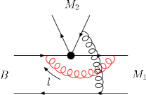
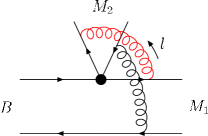
(a)	(b)	(c)
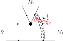
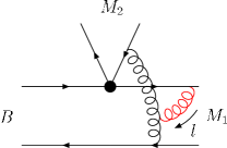
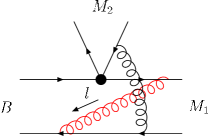
(d)	(e)	(f)

Figure 14: NLO diagrams for Fig. 1(a) that are relevant to the factorization of the $M_{1}$ meson wave function.

Consider all possible attachments of the collinear gluon emitted by the valence quark of $M_{1}$ to other particle lines, which are displayed in Fig. 14. Figure 14(c) contains the four denominators

$$[(k_{2}-l)^{2}+i\epsilon][(P_{1}-k_{1}+l)^{2}+i\epsilon](l^{2}+i\epsilon)[(k_{2}-k+k_{1}-l)^{2}+i\epsilon],$$ (55)

with which the Feynman parameters $x$, $t$, $1-x-y-t$, and $y$ are associated in sequence. It is straightforward to derive

$$M^{2}=(x+y)t(P_{1}-k_{1})\cdot k_{2}+y(1-x-y)k_{1}\cdot k_{2}-yt(P_{1}-k_{1})\cdot k-y(1-y)k_{1}\cdot k.$$ (56)

It is appropriate to integrate out $t$ first, since its coefficient $x(P_{1}-k_{1})\cdot k_{2}+y(P_{1}-k_{1})\cdot(k_{2}-k)>0$ does not flip sign according to the power counting rules. The term from the upper bound $t=1-x-y$, which corresponds to a collinear divergence from $l$ parallel to $P_{1}$, gives

$$M^{2}_{t=1-x-y}=(1-x-y)[(x+y)(P_{1}-k_{1})\cdot k_{2}+yk_{1}\cdot k_{2}-y(P_{1}-k_{1})\cdot k-yk_{1}\cdot k]-xyk_{1}\cdot k.$$ (57)

To get pinched infrared singularities, we must have small $x,y$ due to the large denominators $(k_{2}-l)^{2},\,(k_{2}-k+k_{1}-l)^{2}$. The above expression becomes in the $x,y\to 0$ limit

$$M^{2}_{t=1-x-y}=x(P_{1}-k_{1})\cdot k_{2}+yP_{1}\cdot(k_{2}-k)-xyk_{1}\cdot k>0,$$ (58)

because the third term over the first term is of $O(\lambda^{3})$ even for $k_{1}^{+}\sim O(m_{B})$ ($y$ is of $O(\lambda^{2})$ then). Another term from the lower bound $t=0$ is written as

$$M^{2}_{t=0} = y[(1-x-y)k_{1}\cdot k_{2}-(1-y)k_{1}\cdot k],$$ (59)

$$\approx yk_{1}\cdot(k_{2}-k)>0,$$

in the $x,y\to 0$ limit. The pole structures of Eq. (55) can be analyzed in a way the same as in Sec. II. It will be seen that the interval of $l^{-}$ does not cover the origin, as the contour integration over $l^{+}$ is performed first, or the Glauber divergences associated with the poles of $l^{-}$ cancel each other at leading power in $1/m_{B}$, as $l^{-}$ is integrated out first. In conclusion, Fig. 14(c) does not contain a Glauber divergence.

The analysis of Fig. 14(b) is trivial. Due to the absence of $y$, it is easy to write down

$$M^{2}=xt(P_{1}-k_{1})\cdot(P_{2}-k_{2})>0.$$ (60)

That is, it just provides soft subtraction for Fig. 14(c) at $y\to 0$.

References

- (1) Y. Amhis et al. [Heavy Flavor Averaging Group Collaboration], arXiv:1207.1158 [hep-ex], and online update at http://www.slac.stanford.edu/xorg/hfag.
- (2) C. Chiang et al., Phys. Rev. D 70, 034020 (2004); Y.Y. Charng and H.-n. Li, Phys. Rev. D 71, 014036 (2005); R. Fleischer, S. Recksiegel, and F. Schwab, Eur. Phys. J. C 51, 55 (2007).
- (3) T.N. Pham, arXiv:0910.2561 [hep-ph].
- (4) H.Y. Cheng and C.K. Chua, Phys. Rev. D 80, 074031 (2009).
- (5) C.D. Lü and M.Z. Yang, Eur. Phys. J. C23, 275 (2002).
- (6) R. Zhou, X.D. Gao, and C.D. Lü, Eur. Phys. J. C 72, 1923 (2012).
- (7) M. Beneke and M. Neubert, Nucl. Phys. B675, 333 (2003).
- (8) H.-n. Li and S. Mishima, Phys. Rev. D 73, 114014 (2006).
- (9) W.S. Hou, H.-n. Li, S. Mishima, and M. Nagashima, Phys. Rev. Lett. 98, 131801 (2007).
- (10) A. Soni et al., Phys. Lett. B 683, 302 (2010).
- (11) R. Fleischer, S. Jager, D. Pirjol, and J. Zupan, Phys. Rev. D 78, 111501 (2008), and references therein.
- (12) S. Baek, J.H. Jeon, and C.S. Kim, Phys. Lett. B 664, 84 (2008).
- (13) G. Bhattacharyya, K.B. Chatterjee, and S. Nandi, Phys. Rev. D 78, 095005 (2008).
- (14) R. Mohanta and A.K. Giri, Phys. Rev. D 79, 057902 (2009).
- (15) Q. Chang, X.-Q. Li, and Y.-D. Yang, JHEP 0905, 056 (2009).
- (16) S. Baek, C.-W. Chiang, M. Gronau, D. London, and J.L. Rosner, Phys. Lett. B 678, 97 (2009).
- (17) S. Khalil, A. Masiero, and H. Murayama, Phys. Lett. B 682, 74 (2009).
- (18) K. Huitu and S. Khalil, Phys. Rev. D 81, 095008 (2010).
- (19) K. Cho and S.-h. Nam, Phys. Rev. D 88, 035012 (2013).
- (20) M. Imbeault, S. Baek, and D. London, Phys. Lett. B 663, 410 (2008).
- (21) M. Endo and T. Yoshinaga, Prog. Theor. Phys. 128, 1251 (2012).
- (22) M. Beneke, J. Rohrer, and D. Yang, Nucl. Phys. B774, 64 (2007).
- (23) H.J. Lipkin, arXiv:1102.4700 [hep-ph].
- (24) Y.Y. Keum, H.-n. Li, and A.I. Sanda, Phys Lett. B 504, 6 (2001); Phys. Rev. D 63, 054008 (2001).
- (25) C.D. Lü, K. Ukai, and M.Z. Yang, Phys. Rev. D 63, 074009 (2001).
- (26) H.-n. Li, S. Mishima, and A.I. Sanda, Phys. Rev. D 72, 114005 (2005).
- (27) Y.L. Zhang, X.Y. Liu, Y.Y. Fan, S. Cheng, and Z.J. Xiao, Phys. Rev. D 90, 014029 (2014).
- (28) M. Beneke and D. Yang, Nucl. Phys. B736, 34 (2006); M. Beneke and S. Jager, Nucl. Phys. B751, 160 (2006); G. Bell, Nucl. Phys. B795, 1 (2008); V. Pilipp, Nucl. Phys. B794, 154 (2008); M. Beneke, T. Huber, and X.Q. Li, Nucl. Phys. B832, 109 (2010).
- (29) H.-n. Li and S. Mishima, Phys. Rev. D 83, 034023 (2011).
- (30) J. Collins and J.W. Qiu, Phys. Rev. D 75, 114014 (2007); J. Collins, arXiv:0708.4410 [hep-ph].
- (31) G.P. Lepage and S.J. Brodsky, Phys. Lett. B 87, 359 (1979); S. Nussinov and R. Shrock, Phys. Rev. D 79, 016005 (2009); M. Duraisamy and A.L. Kagan, Eur. Phys. J. C 70, 921 (2010).
- (32) M. Petric [Belle Collaboration], talk presented at the 37th International Conference on High Energy Physics at Valencia Spain, July 2-9, 2014.
- (33) C.K. Chua, W.S. Hou, and K.C. Yang, Phys. Rev. D 65, 096007 (2002); A.B. Kaidalov and M.I. Vysotsky, Phys. Lett. B 652, 203 (2007); M.I. Vysotsky, arXiv:0901.2245; A.F. Falk et al., Phys. Rev. D 57, 4290 (1998).
- (34) C.K. Chua, Phys. Rev. D 78, 076002 (2008).
- (35) C.-p. Chang and H.-n. Li, Eur. Phys. J. C 71, 1687 (2011); H.-n. Li, arXiv:1009.3610 [hep-ph].
- (36) M. Nagashima and H.-n. Li, Phys. Rev. D 67, 034001 (2003).
- (37) H.-n. Li, Y.L. Shen, and Y.M. Wang, Phys. Rev. D 85, 074004 (2012).
- (38) G. Buchalla, A. J. Buras, and M. E. Lautenbacher, Rev. Mod. Phys., 68, 1125 (1996).
- (39) H.-n. Li and B. Tseng, Phys. Rev. D 57, 443 (1998).
- (40) H.-n. Li, Phys. Rev. D 64, 014019 (2001).
- (41) H.-n. Li and S. Mishima, Phys. Rev. D 74, 094020 (2006).
- (42) J. Beringer et al. (Particle Data Group), Phys. Rev. D 86, 010001 (2012), and online update at http://pdg.lbl.gov/.
- (43) P. Ball, G.W. Jones, and R. Zwicky, Phys. Rev. D 75, 054004 (2007).
- (44) T. Kurimoto, H.-n. Li, and A.I. Sanda, Phys. Rev. D 65, 014007 (2001).
- (45) M. Ciuchini, E. Franco, G. Martinelli, M. Pierini, and L. Silvestrini, Phys. Lett. B 674, 197 (2009).
- (46) S. Baek, C.-W. Chiang, and D. London, Phys. Lett. B 675, 59 (2009).
- (47) C.-p. Chang and H.-n. Li, Phys. Lett. B 726, 262 (2013).
- (48) C.S. Lam and W.K. Tung, Phys. Rev. D 18, 2447 (1978).
- (49) S. Falciano et al. [NA10 Collaboration], Z. Phys. C 31, 513 (1986).
- (50) M. Guanziroli et al. [NA10 Collaboration], Z. Phys. C 37, 545 (1988).
- (51) J.S. Conway et al., Phys. Rev. D 39, 92 (1989).
- (52) L.D. Landau, Nucl. Phys. 13, 181 (1959).