Supersymmetric multiplex networks described by coupled Bose and Fermi statistics

Abstract

Until now, no simple symmetries have been detected in complex networks. Here we show that, in growing multiplex networks the symmetries of multilayer structures can be exploited by their dynamical rules, forming supersymmetric multiplex networks described by coupled Bose-Einstein and Fermi-Dirac quantum statistics. The supersymmetric multiplex is formed by layers which are scale-free networks and can display a Bose-Einstein condensation of the links. To characterize the complexity of the supersymmetric multiplex using quantum information tools, we extend the definition of the network entanglement entropy to the layers of multiplex networks. Interestingly we observe a very simple relation between the entanglement entropies of the layers of the supersymmetric multiplex network and the entropy rate of the same multiplex network. This relation therefore connects the classical non equilibrium growing dynamics of the supersymmetric multiplex network with its quantum information static characteristics.

I Introduction

Recently, the relation among complex networks, their geometry and evolution RMP ; Newman_rev ; Boccaletti2006 , and more traditional fields of physics such as quantum physics and quantum communication Cirac ; Calsamiglia ; Sachdev ; Ising ; Hubbard ; JCH , quantum information Quantuminformation , cosmology Cosmology and quantum gravity Rovelli ; Rovelli2 ; triangulations are starting to attract the interest of scientists.

For instance, an interesting aspect of complex network evolution is that in major examples of realistic models for complex networks growth, quantum statistics emerge as important distributions determining the network dynamics. In fact, the evolution of scale-free networks with fitness of the nodes Fitness is described by the Bose-Einstein statistics and this model can be therefore mapped to a Bose gas. In correspondence of the Bose-Einstein condensation Bose of the Bose gas, the network topology undergoes a major structural condensation transition in which a node is linked to a finite fraction of links. This model can explain the emergence of “super-hubs” in complex networks and the “winner-takes-all” phenomenon. Interestingly the evolution of Cayley trees with fitness of the nodes, is determined by the Fermi-Dirac statistics Fermi ; Complex . In addition to that, it has also been found that ensembles of complex networks have been shown to be related with quantum statistics Garlaschelli . Finally, it has been shown that random geometric networks on a hyperbolic space can show a scale-free network topology Hyperbolic ; Navigability and that growing networks in hyperbolic space define the so called “network cosmology” Cosmology . From the quantum information perspective, complex networks encode relevant information in their structures, and new quantum entropy measures have been proposed in order to characterize and quantify this information Vonneuman ; Garnerone ; Jesus2 .Moreover, the quantum random walk can be used to propose different definitions of quantum PageRank on networks Garneronegoogle ; Jesus1 ; Faccin ; Zimboras ; Caldarelli .

Multiplex networks are multilayer network structures that are attracting large interest PhysicsReports ; Kivela . In fact they are able to describe several types of interactions between the same set of nodes. For example, social networks, where the same people are connected by different means of communications, or different types of social ties, like friendship, collaboration, co-authorship, and so on are better described by multiplex networks. Similarly, if we want to describe diffusion in transportation networks we need to consider the multiplex nature of the underlying transportation networks, where a given location can be linked to other locations by different types of transportation, train, bus, airplane etc. Finally, in brain networks the large variety of neuron types and types of interactions between them, will not be fully understood if the multilayer approach is not adopted Bullmore ; Makse ; Liaisons . Multilayer have a highly non trivial structure including communities Mason and many different types of encoded structural correlations PRE ; Goh ; Vito . Recently some quantum information measures such as the Von Neumann entropy of single networks Vonneuman have been extended to multilayer networks in order to quantify their complexity Math .

Multiplex networks are formed by layers that are usually scale-free and have a number of nodes that increases in time. For these reasons their evolution can be described by growing multiplex networks models Growth1 ; Growth2 ; Nonlinear . In single layer networks growing network models BA ; Fitness ; Bose are able to explain the spontaneous emergence of scale-free degree distribution. In particular the most fundamental growing network model, the Barabási-Albert (BA) model BA includes only two dynamical rules: growth and preferential attachment, meaning that at each time a new node is added to the network and it attaches links preferentially to high degree nodes. Just these two elements of the model have been shown to be responsible for a scale-free degree distribution of exponent $\gamma=3$. An important element determining network evolution is the intrinsic quality of the nodes, determining their fitness that make them more likely to acquire new links, with respect to other nodes with the same degree Fitness . The dynamics of single growing scale-free networks with fitness of the nodes can be mapped to a Bose gas Bose giving rise to the intriguing phenomenon of the Bose-Einstein condensation, while growing Cayley trees with fitness of the nodes can be mapped to a Fermi gasFermi by using a similar mathematical formalism.

In the context of multiplex networks, growing multiplex networks models have been shown to generate multiplex networks with different degree distributions in the different layers, and different pattern of correlations PRE ; Goh ; Vito between the degrees of the same node in different layers Growth1 ; Growth2 ; Nonlinear . Nevertheless the role of the fitness of the nodes on growing multiplex networks models has not yet been explored. Here we combine the process of link addition and the process of rewiring of the links in presence of an intrinsic fitness of the nodes. We show that the network growth can exploit the symmetries of the multiplex networks and we can generate scale-free supersymmetric multiplex networks described by coupled Fermi-Dirac and Bose-Einstein statistics. Moreover, we explore the information content of these structures with quantum information tools by extending the definition of entanglement entropy of single networks Garnerone to multiplex structures. To this end we map each each network in a given layer to a quantum network state and we describe the complexity of each layer of the multiplex networks by calculating the entanglement entropies of these quantum states. Finally we relate the entanglement entropies of the layers of the supersymmetric multiplex network to the entropy rate of the multiplex network. The entropy rate Entropyrate of the supersymmetric multiplex model describes the rate at which the typical number of multiplex networks, which can be realized during the dynamics, grows in time. Therefore here we show that the entanglement entropies of the layers of the supersymmetric network, which extract information form a snapshot of the multiplex network using quantum information tools, have a very simple relation with the entropy rate of the same supersymmetric multiplex network, describing the classical non-equilibrium dynamics of the multilayer structure.

The paper is structured as follows: In section II we define the supersymmetric multiplex model and we provide its mean-field solution. In section III we characterize the supersymmetric multiplex structural properties. In section IV we define the entropy rate of the supersymmetric multiplex network. In section V evaluate the entanglement entropies of the layers of the supersymmetric multiplex network. In section VI we relate the entanglement entropies of the layers of the supersymmetric multiplex network with its entropy rate. Finally in section VII we give the conclusions.

We note here that for simplicity in the main text of the paper we consider only the case of a duplex (i.e. a multiplex with $M=2$), but the analysis can be easily extended to a multiplex with a generic value of the number of layers $M$. Therefore in the appendix the extension to supersymmetric multiplex networks with generic value of $M$ is discussed.

II supersymmetric multiplex network model

II.1 The supersymmetric multiplex evolution

A multiplex network is a multilayer system formed by $N$ nodes having a copy (or replica) in each of the $M$ layers, and $M$ layers formed by different networks of interactions between the $N$ nodes. Here we assume that each node $i$ has quenched quality quantified by the quenched parameter $\epsilon_{i}\in(0,1)$ called the energy of the node and we indicate by

$$\eta_{i}=e^{-\beta\epsilon_{i}}$$ (1)

the fitness of the node $i$, determined both by its energy and a global parameter $\beta>0$. On single layers it has been shown Fitness ; Bose that the fitness of the nodes is able to explain how some nodes (the more fit) acquire links at a faster rate than others, as observed in a variety of complex networks, including the Internet and the World-Wide-Web. In particular, in these models it is assumed that each new node links preferentially to nodes of high degree and high fitness, with a probability $\Pi_{i}$ that it attaches a new link to a node $i$ given by

$$\Pi_{i}=\frac{\eta_{i}k_{i}}{\sum_{j}\eta_{j}k_{j}}=\frac{e^{-\beta\epsilon_{i}}k_{i}}{\sum_{j}e^{-\beta\epsilon_{j}}k_{j}},$$ (2)

where $k_{i}$ is the degree of node $i$, in this way generalizing the dynamics of the famous BA model BA in which the preferential attachment is only driven by the degree of the nodes.

When considering the evolution of technological, social or transportation multilayer networks, a similar mechanism can be taken into account. Nevertheless t,he new links of a given layer might be added also according to a preferential attachment mechanism deriving from the popularity of a node in another layer. This model the case in which a popular node in one layer attracts also links in another layer. Moreover, it can also happen that, instead, the popularity of a node in a layer is modulated by a process of rewiring of the links, and that links attached to popular nodes in one layer are more likely to be rewired. This could mimic the case in which the connectivities of hubs are damped by the process of link rewiring. We consider for simplicity a multiplex networks formed by $M=2$ layers and we describe its evolution as a growing multiplex network model in which each node has a given energy and corresponding fitness. Specifically, we consider the case in which in the dynamics in the two networks is not symmetrical. In one layer new links are exclusively added according to a generalized preferential attachment which rewards high fitness nodes of high degree in either one of the layers, and in the other layer the links are attached but also rewired in such a way to reduce the growth of the degree of high fitness nodes in that layer. This model can be generalized to a multiplex networks with larger number of layers in which the layer can be divided in two groups, each group of layer behaving in a similar way. In order to keep the description of the model simple we now focus on the case in which $M=2$, discussing in the appendix the generalization to the general value of $M$. We start at $t=0$ from a small set of nodes $N_{0}$ connected in both layers. Each node $i$ of the network has degrees $k^{[1]}_{i},k^{[2]}_{i}$ respectively in layer 1 and layer 2, and energy $\epsilon_{i}$ drawn from a $g(\epsilon)$ distribution. At each time $t$ we add a node to the multiplex network, each node has two replicas nodes, one on each layer. Moreover, each replica node is initially attached to $m$ existing nodes in the same layer. In the following we will indicate with $l$ the number of network changes, i.e. links additions or link rewirings, occurring in each layer starting from time $t=1$. After time $t$ we will have $l=mt$. For each network change in layer 1 we follow the subsequent procedure:

• We extract a number $\sigma^{[1]}_{l}=1,2$. The event $\sigma^{[1]}_{l}=1$ occurs with probability $p^{[1]}(1)=\alpha$ while the event $\sigma_{l}^{[1]}=2$ occurs with probability $p^{[1]}(2)=1-\alpha$.

• If $\sigma^{[1]}_{l}=1$ the new node is attached in layer 1 to a node $i^{[1]}_{l}$ chosen with probability

  $$\Pi^{[1,1]}\left(i_{l}^{[1]}=i\right)=\frac{e^{-\beta\epsilon_{i}}k_{i}^{[1]}}{\sum_{j}e^{-\beta\epsilon_{j}}k_{j}^{[1]}},$$ (3)

  i.e. it will be attached preferentially to nodes with low energy and high degree in layer 1, according to a generalized preferential attachment. Instead, if $\sigma^{[1]}_{l}=2$ the new node is attached in layer 1 to a node $i^{[1]}_{l}$ chosen with probability

  $$\Pi^{[1,2]}\left(i_{l}^{[1]}=i\right)=\frac{e^{-\beta\epsilon_{i}}k_{i}^{[2]}}{\sum_{j}e^{-\beta\epsilon_{j}}k_{j}^{[2]}},$$ (4)

  i.e. will be attached preferentially to nodes with low energy and high degree in layer 2, according to a generalized preferential attachment.

For each network change in layer 2 we follow the subsequent procedure:

• We extract a number $\sigma^{[2]}_{l}=1,2$. The event $\sigma^{[2]}_{l}=1$ occurs with probability $p^{[2]}(1)=1-\alpha$ while the event $\sigma_{l}^{[2]}=2$ occurs with probability $p^{[2]}(2)=\alpha$.

• If $\sigma^{[2]}_{l}=1$ the new node will be attached, in layer 2, to a node $i_{l}^{[2]}$ chosen with probability

  $$\Pi^{[2,1]}\left(i_{l}^{[2]}=i\right)=\frac{e^{-\beta\epsilon_{i}}k_{i}^{[1]}}{\sum_{j}e^{-\beta\epsilon_{j}}k_{j}^{[1]}}.$$ (5)

  Instead, if $\sigma^{[2]}_{l}=2$ a random link of a node $i^{[2]}_{l}$ chosen with probability

  $$\Pi^{[2,2]}\left(i_{l}^{[2]}=i\right)=\frac{e^{-\beta\epsilon_{i}}k_{i}^{[2]}}{\sum_{j}e^{-\beta\epsilon_{j}}k_{j}^{[2]}}$$ (6)

  is rewired, i.e. it is detached from node $i_{l}^{[2]}$ and attached to the new node of the network.

Therefore the network is determined by the sequence of the values $\{\sigma^{[1]}_{l},i_{l}^{[1]}\sigma^{[2]}_{l},i_{l}^{[2]}\}$ that fully determines the evolution of the multiplex network given the initial condition.

II.2 Mean-field solution of the supersymmetric multiplex model

When studying growing networks with preferential attachment, in general large attention is given to the degree sequence of the network. In order to predict the degree distribution of these models, mean-field approaches have been extensively studied, finding that in general they give a very good prediction of the structural properties of the network Doro_book . In this paper we analyse the supersymmetric multiplex model with the mean-field theory leaving to subsequent works the analysis with the master equation approach. In order to check the validity of the approach we then compare the analytical results to simulations as discussed in Section III. In the mean-field approach, one assumes that the degree of each node has no fluctuations, and therefore identifies the degrees $k^{[1]}_{i},k^{[2]}_{i}$ at time $t$ with their average over the multiplex network realization. Moreover this approximation is also called the continuous approximation because it is assumed that both the degrees of the nodes and the time are continuous variables. Therefore the mean-field equations for the supersymmetric multiplex model read

$$\frac{dk_{i}^{[1]}}{dt}=me^{-\beta\epsilon_{i}}\left[\frac{\alpha}{\sum_{j}e^{-\beta\epsilon_{j}}k_{j}^{[1]}}k_{i}^{[1]}+\frac{(1-\alpha)}{\sum_{j}e^{-\beta\epsilon_{j}}k_{j}^{[2]}}k_{i}^{[2]}\right],$$

$$\frac{dk_{i}^{[2]}}{dt}=me^{-\beta\epsilon_{i}}\left[\frac{(1-\alpha)}{\sum_{j}e^{-\beta\epsilon_{j}}k_{j}^{[1]}}k_{i}^{[1]}-\frac{\alpha}{\sum_{j}e^{-\beta\epsilon_{j}}k_{j}^{[2]}}k_{i}^{[2]}\right].$$ (7)

Using an approach similar to the one used in the Bianconi-Barabási model Bose , we will assume self consistently that

$$\lim_{t\to\infty}\frac{\sum_{j}e^{-\beta\epsilon_{j}}k_{j}^{[1]}}{mt} = c_{1},$$

$$\lim_{t\to\infty}\frac{\sum_{j}e^{-\beta\epsilon_{j}}k_{j}^{[2]}}{mt} = c_{2},$$ (8)

where $c_{1}$ and $c_{2}$ are constants independent of the network realization. Therefore, asymptotically in time we have

$$\sum_{j}e^{-\beta\epsilon_{j}}k_{j}^{[1]} \simeq mtc_{1},$$

$$\sum_{j}e^{-\beta\epsilon_{j}}k_{j}^{[2]} \simeq mtc_{2}.$$ (9)

If we define the vector of the degree of each node as

$${\bf k}_{i}=\left(\begin{array}[]{c}k^{[1]}_{i}(t)\\ k^{[2]}_{i}(t)\end{array}\right),$$ (11)

and we substitute for $t\gg 1$ the asymptotic expression for the normalization sums Eq. $(\ref{asymptotics})$ we obtain that the mean-field Eqs. $(\ref{mf0})$ can be written as

$$\frac{d{\bf k}_{i}}{dt}=\frac{e^{-\beta\epsilon_{i}}}{t}{\bf A}{\bf k}_{i},$$ (12)

where the matrix ${\bf A}$ is defined as

$${\bf A} = \left(\begin{array}[]{cc}\alpha/c_{1}&(1-\alpha)/c_{2}\\ (1-\alpha)/c_{1}&-\alpha/c_{2}\end{array}\right).$$ (14)

The solution of Eq. $(\ref{mfs})$ is given in terms of the eigenvalue and the eigenvector of the matrix ${\bf A}$.These eigenvalue are respectively positive and negative for every value of the parameter $\alpha$ of the model. We will indicate the eigenvalues of ${\bf A}$ as $\lambda_{+}$ and $\lambda_{-}$ in correspondence of their sign. These eigenvalues are given by

$$\lambda_{+}=\frac{1}{2}\left[\left(\frac{\alpha}{c_{1}}-\frac{\alpha}{c_{2}}\right)+\sqrt{\Delta}\right],$$

$$\lambda_{-}=\frac{1}{2}\left[\left(\frac{\alpha}{c_{1}}-\frac{\alpha}{c_{2}}\right)-\sqrt{\Delta}\right],$$ (15)

with

$$\Delta=\left(\frac{\alpha}{c_{1}}-\frac{\alpha}{c_{2}}\right)^{2}+4\frac{\alpha^{2}+(1-\alpha)^{2}}{c_{1}c_{2}}.$$ (16)

We have therefore that the constants $c_{1}$ and $c_{2}$ can be expressed as a function of $\lambda_{+}$ and $\lambda_{-}$ as

$$c_{1} = \frac{(1-\alpha)^{2}+\alpha^{2}}{2\alpha}\left[\left(\frac{1}{\lambda_{+}}+\frac{1}{\lambda_{-}}\right)+\sqrt{\Lambda}\right],$$

$$c_{2} = \frac{(1-\alpha)^{2}+\alpha^{2}}{2\alpha}\left[-\left(\frac{1}{\lambda_{+}}+\frac{1}{\lambda_{-}}\right)+\sqrt{\Lambda}\right],$$ (17)

with

$$\Lambda = \left(\frac{1}{\lambda_{+}}+\frac{1}{\lambda_{-}}\right)^{2}-\frac{4\alpha^{2}}{[(1-\alpha)^{2}+\alpha^{2}]}\frac{1}{\lambda_{+}\lambda_{-}}.$$ (18)

Moreover, we indicate by ${\bf u^{+}}=(u_{1}^{+},u_{2}^{+})$ and ${\bf u^{-}}=(u_{1}^{-},u_{2}^{-})$ the eigenvectors corresponding respectively to the eigenvalues $\lambda_{+}$ and $\lambda_{-}$. The components of these eigenvectors are given by

$$u^{+}_{1} = \frac{c_{1}}{2(1-\alpha)}\left(\frac{\alpha}{c_{2}}+\frac{\alpha}{c_{1}}+\sqrt{\Delta}\right),$$

$$u^{+}_{2} = 1,$$

$$u^{-}_{1} = \frac{c_{1}}{2(1-\alpha)}\left(\frac{\alpha}{c_{2}}+\frac{\alpha}{c_{1}}-\sqrt{\Delta}\right),$$

$$u^{-}_{2} = 1.$$ (19)

Therefore, solving the Eqs. $(\ref{mfs})$ the degrees of node $i$ in the two layers can be calculated in the mean-field approximation to be

$${\bf k}_{i}(t)=d^{+}{\bf u^{+}}\left(\frac{t}{t_{i}}\right)^{e^{-\beta\epsilon_{i}}\lambda_{+}}+d^{-}{\bf u^{-}}\left(\frac{t}{t_{i}}\right)^{-e^{-\beta\epsilon_{i}}\lambda_{-}},$$ (20)

where $t_{i}$ is the time at which the node $i$ is arrived in the network and where $d^{-}$ and $d^{+}$ are constants determined by the initial condition ${\bf k}_{i}(t_{i})=m{\bf 1}$ where ${\bf 1}$ is the column vector of components $(1,1)$. Starting from Eq. $(\ref{k1})$, the initial condition can be also written as

$${\bf k}_{i}(t_{i})=m{\bf 1}={\bf U}{\bf d},$$ (21)

where ${\bf U}$ is the matrix with column vectors given by the eigenvectors ${\bf u}^{+}$ and ${\bf u}^{-}$ i.e.

$${\bf U}=\left(\begin{array}[]{cc}u_{1}^{+}&u_{1}^{-}\\ u_{2}^{+}&u_{2}^{-}\end{array}\right),$$ (23)

and the column vector ${\bf d}$ has components ${\bf d}=(d^{+},d^{-})$. This equation can always be solved finding that the constants $d^{+}$ and $d^{-}$ are given by

$${\bf d} = m{\bf U}^{-1}{\bf 1}$$ (25)

$$= \frac{m}{u_{1}^{+}u_{2}^{-}-u_{1}^{-}u_{2}^{+}}\left(\begin{array}[]{c}u_{2}^{-}-u_{1}^{-}\\ u_{1}^{+}-u_{2}^{+}\end{array}\right).$$

Note that the denominator of Eq. $(\ref{dp})$ is always positive definite and never singular since we have $u_{2}^{-}>0,u_{2}^{+}>0,u_{1}^{+}>0$ but $u_{1}^{-}<0$. Having fixed the constant $d^{+}$ and $d^{-}$, we can rewrite Eq. $(\ref{k1})$ as

$${\bf k}_{i}={\bf B}{\bf v}_{i}$$ (26)

with ${\bf v}_{i}$ indicating the column vector

$${\bf v}_{i}=\left(\begin{array}[]{c}\left(\frac{t}{t_{i}}\right)^{e^{-\beta\epsilon_{i}}\lambda_{+}}\\ \left(\frac{t}{t_{i}}\right)^{e^{-\beta\epsilon_{i}}\lambda_{-}}\end{array}\right),$$ (29)

and the matrix ${\bf B}$ given by

$${\bf B}=\left(\begin{array}[]{cc}d^{+}u_{1}^{+}&d^{-}u_{1}^{-}\\ d^{+}u_{2}^{+}&d^{-}u_{2}^{-}\end{array}\right).$$ (31)

Therefore we have also that

$${\bf v}_{i}={\bf B}^{-1}{\bf k}_{i}$$ (32)

with

$${\bf B}^{-1}=\frac{1}{m}\left(\begin{array}[]{cc}\frac{u_{2}^{-}}{u_{2}^{-}-u_{1}^{-}}&-\frac{u_{1}^{-}}{u_{2}^{-}-u_{1}^{-}}\\ -\frac{u_{2}^{+}}{u_{1}^{+}-u_{2}^{+}}&\frac{u_{1}^{+}}{u_{1}^{+}-u_{2}^{+}}\end{array}\right)$$ (34)

which is always well defined except for values in parameter space of zero Lebesgue measure where $u^{+}_{1}=1$. Since $\lambda_{+}$ and $\lambda_{-}$have respectively positive and negative sign, Eq. $(\ref{lin})$ defines the two linear combination of the degrees $k^{[1]}$ and $k^{[2]}$ that respectively increases and decreases as a power-law of time. Therefore we have found the solution of the model, once the constants $c_{1}$ and $c_{2}$ are given. In order to find the correct values of the constants $c_{1}$ and $c_{2}$ given by Eqs.$(\ref{selfc0})$, we need to close our self-consistent argument. Since we have assumed that the constants $c_{1}$ and $c_{2}$ are independent on the network realization, determined in the mean-field approximation by the quenched disorder of the assignment of the energies to the nodes, the constants $c_{1}$ and $c_{2}$ can be evaluated performing the following limits:

$$\lim_{t\to\infty}\frac{\left\langle{\sum_{j}e^{-\beta\epsilon_{j}}k_{j}^{[1]}}\right\rangle}{mt} = c_{1},$$

$$\lim_{t\to\infty}\frac{\left\langle{\sum_{j}e^{-\beta\epsilon_{j}}k_{j}^{[2]}}\right\rangle}{mt} = c_{2},$$ (35)

where in Eqs. $(\ref{selfc1})$ the average is performed over the distribution of the energies of the nodes. Therefore, by multiplying each equation of Eq. $(\ref{k2})$ by $e^{-\beta\epsilon_{i}}$, integrating over the continuous time $t_{i}$, and averaging over the $g(\epsilon)$ distribution we get that the self consistent equations determining the constants $c_{1}$ and $c_{2}$, or equivalently $\lambda_{+}$ and $\lambda_{-}$, are given by

$$m{\bf c}={\bf B}{\bf J}$$ (36)

where the column vector ${\bf J}=(J_{+},J_{-})$ has component given by

$$J_{+} = \int d\epsilon g(\epsilon)\frac{1/\lambda_{+}}{e^{\beta\epsilon}/\lambda_{+}-1},$$

$$J_{-} = \int d\epsilon g(\epsilon)\frac{1/\lambda_{-}}{e^{\beta\epsilon}/\lambda_{-}-1}.$$ (37)

Inverting Eqs. $(\ref{dir})$ we can express ${\bf J}$ as

$${\bf J} = m{\bf B}^{-1}{\bf c}=\left(\begin{array}[]{c}\frac{(c_{1}u_{2}^{-}-c_{2}u_{1}^{-})}{u_{2}^{-}-u_{1}^{-}}\\ \frac{(c_{2}u_{1}^{+}-c_{1}u_{2}^{+})}{u_{1}^{+}-u_{2}^{+}}\\ \end{array}\right).$$ (39)

By defining the two constants $\mu_{B}$ and $\mu_{F}$, as in the following,

$$\lambda^{+}=e^{\beta\mu_{B}}$$

$$-\lambda^{-}=e^{\beta\mu_{F}}$$ (40)

and multiplying $J^{+}$ by $\lambda^{+}$ and $J^{-}$ by $-\lambda^{-}$ we get the following self-consistent equation, fixing the “chemical potentials” $\mu_{B}$ and $\mu_{F}$,

$$I_{B}=\int d\epsilon g(\epsilon)\frac{1}{e^{\beta(\epsilon-\mu_{B})}-1}=G_{B},$$

$$I_{F}=\int d\epsilon g(\epsilon)\frac{1}{e^{\beta(\epsilon-\mu_{F})}+1}=G_{F},$$ (41)

with $G_{B}$ and $G_{F}$ independent on the energy distribution and only function of the inverse temperature $\beta$ and the two “chemical potentials” $\mu_{B}$ and $\mu_{F}$. In fact we have,

$${\bf G} = \left(\begin{array}[]{c}G_{B}\\ G_{F}\end{array}\right)=\left(\begin{array}[]{c}\frac{(c_{1}u_{2}^{-}-c_{2}u_{1}^{-})}{u_{2}^{-}-u_{1}^{-}}\lambda_{+}\\ \frac{(c_{1}u_{2}^{+}-c_{2}u_{1}^{+})}{u_{1}^{+}-u_{2}^{+}}\lambda_{-}\\ \end{array}\right).$$ (44)

From the self-consistent Eq. $(\ref{selfq})$ the two constants $\mu_{B}$ and $\mu_{F}$ can be interpreted as ‘chemical potentials” of coupled Bose and Fermi gases and fully determine the evolution of the supersymmetric multiplex network, as long as the equations can be satisfied. Only the left hand side of the Eqs. $(\ref{selfq})$ depends on the energy distribution $g(\epsilon)$ while the right hand side does not depend on it. Moreover the quantities $G_{B}$ and $G_{F}$ depend on both the chemical potential $\mu_{B}$ and $\mu_{F}$ and can be explicitly expressed as

$$G_{B} = e^{\beta\mu_{B}}\frac{(2-\alpha)e^{-\beta\mu_{B}}+\alpha e^{-\beta\mu_{F}}+(1-2\alpha)\sqrt{\Lambda}}{\alpha e^{-\beta\mu_{B}}+(2-\alpha)e^{-\beta\mu_{F}}+(1-2\alpha)\sqrt{\Lambda}}\times$$

$$\times\frac{(1-\alpha)^{2}+\alpha^{2}}{2\alpha}\left[-e^{-\beta\mu_{B}}+e^{-\beta\mu_{F}}+\sqrt{\Lambda}\right],$$

$$G_{B} = e^{\beta\mu_{F}}\frac{-\alpha e^{-\beta\mu_{B}}+(2-\alpha)e^{-\beta\mu_{F}}+(1-2\alpha)\sqrt{\Lambda}}{-(2-\alpha)e^{-\beta\mu_{B}}+\alpha e^{-\beta\mu_{F}}+(1-2\alpha)\sqrt{\Lambda}}\times$$

$$\times\frac{(1-\alpha)^{2}+\alpha^{2}}{2\alpha}\left[-e^{-\beta\mu_{B}}+e^{-\beta\mu_{F}}+\sqrt{\Lambda}\right],$$

where $\Lambda$ is given by

$$\Lambda=\left(e^{-\beta\mu_{B}}-e^{-\beta\mu_{F}}\right)^{2}+\frac{4\alpha^{2}}{[(1-\alpha)^{2}+\alpha^{2}]}e^{-\beta(\mu_{B}+\mu_{F})}.$$ (45)

The self-consistent Eqs. $(\ref{selfq})$ that fix the chemical potential $\mu_{B}$ and $\mu_{F}$ fully determine the mean-field solution of this model. In the supersymmetric multiplex network, nevertheless there can be two phenomena that implies a breakdown of this solution. On one side we can observe a condensation of the links in correspondence of the regime of high values of $\beta$ where the Eqs.$(\ref{selfq})$ do not have a solution. This phenomenon will be discussed more in depth in the next section. On the other side, it is possible to observe in the model stochastic effects that are not captured by the mean-field solution.

III Structural properties of the supersymmetric multiplex network

The mean-field solution of the model well capture the main characteristics of the supersymmetric multiplex as long as $\alpha$ is not too large. In fact we found very good agreement of the mean-field theory with the simulation results as long as $\alpha$ is lower than $0.5$. For higher values of $\alpha$ in the second layer the rewiring process has a higher rate of the process of addition of new links and therefore non-trivial stochastic effects set in that are not captured by the mean-field solution. For this reason, here we focus on the regime $\alpha<0.5$, where we find very good agreement between the theory and the simulations results. We will describe the structural properties of the supersymmetric multiplex networks, covering the degree distribution of the networks in the two layers, different types of correlations typical of multiplex networks, and we will describe the phenomenology related to the supersymmetric multiplex condensation transition in which one node acquires a finite fraction of all the links in both layers.

III.1 Degree distribution

The degree distribution in the network is scale-free in both layers, as predicted by the mean-field solution. In fact if we consider the dynamical Eq. (20) for the degree $k^{[1]}_{i}$ and the degree $k^{[2]}_{i}$ and we take only the leading term in the limit $t\gg 1$ we found

$$k^{[1]}_{i}\simeq d^{+}u_{1}^{+}\left(\frac{t}{t_{i}}\right)^{e^{-\beta(\epsilon-\mu_{B})}},$$

$$k^{[2]}_{i}\simeq d^{+}u_{2}^{+}\left(\frac{t}{t_{i}}\right)^{e^{-\beta(\epsilon-\mu_{B})}}.$$ (46)

Therefore, using the same mean-field arguments that are used to show that growing complex networks with preferential attachment are scale-free BA ; Bose , we can approximate the degree distributions $P^{[1]}(k)$ and $P^{[2]}(k)$ in the two layers as

$$P^{[1]}(k)\propto\int d\epsilon g(\epsilon)e^{\beta(\epsilon-\mu_{B})}\left(\frac{d^{+}u_{1}^{+}}{k}\right)^{e^{\beta(\epsilon-\mu_{B})}}\frac{1}{k},$$

$$P^{[2]}(k)\propto\int d\epsilon g(\epsilon)e^{\beta(\epsilon-\mu_{B})}\left(\frac{d^{+}u_{2}^{+}}{k}\right)^{e^{\beta(\epsilon-\mu_{B})}}\frac{1}{k}.$$ (47)

These expression reveals that the degree distributions in the two layers can be seen as a convolution of power-law networks with exponents $\gamma(\epsilon)=e^{\beta(\epsilon-\mu_{B})+1}>2$. In Figure 1 we show the degree distribution of the two layers for $g(\epsilon)=(\theta+1)\epsilon^{\theta}$ and $\theta=0.5$ for different values of $\beta=0.,1,5$. The mean-field theory valid as long as the supersymmetric multiplex is not condensed, is in very good agreement with the simulation results.

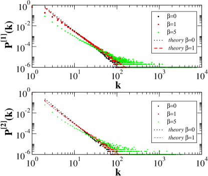
Figure 1: The degree distributions $P^{[1]}(k)$ and $P^{[2]}(k)$ in the two layers of the supersymmetric network. The data is shown for networks of $N=10^{4}$ nodes with energy distribution $g(\epsilon)=(1+\theta)\epsilon^{\theta}$ and $\theta=0.5$, $\alpha=0.3$, $\beta=0,1,5$. The curves are averaged over $100$ multiplex networks realizations.The lines indicate the mean-field expectation for $\beta=0$ and $\beta=1$ and are in very good agreement with the simulation results. The degree distribution for $\beta=5$ is a typical degree distribution below the condensation transition where very big hubs emerge in the network.

III.2 Multilayer degree correlations

In the multiplex networks one relevant correlation is between the degrees of the replica nodes. In particular in a duplex it is interesting to investigate if a hub in a network is also typically a hub in the other network or if it is typically a low degree node. In the supersymmetric multiplex network model, we observe that for $\alpha<0.5$, these correlations are positive. In fact in the mean-field solution, approximating the degrees $k^{[1]}_{i}$ and $k^{[2]}_{i}$ for $t\to\infty$ as in Eq. $(\ref{k12})$, we have

$$k^{[2]}_{i}=\frac{u_{2}^{+}}{u_{1}^{+}}k^{[1]}_{i},$$ (48)

i.e. the degree of layer 2 is positively and linearly correlated with the degree in layer 1. In order to compare this mean-field expectations with the simulation results, we measure from the simulations results the average degree in layer 2 conditioned on the degree in layer 1, i.e. $\left\langle{k^{[2]}|k^{[1]}}\right\rangle$. This quantity characterizes the degree correlation in the multiplex network and is defined as

$$\left\langle{k^{[2]}|k^{[1]}}\right\rangle=\sum_{k^{[2]}}k^{[2]}P(k^{[2]}|k^{[1]}),$$ (49)

where $P(k^{[2]}|k^{[1]})$ is the conditional distribution of having a node of degree $k^{[2]}$ in layer 2 given that it has degree $k^{[1]}$ in layer 1. Since in the mean-field approximation the degrees of nodes are deterministic variables, the mean-field expectation for $\left\langle{k^{[2]}|k^{[1]}}\right\rangle$ is given by Eq $(\ref{k2k1c})$. In Figure 2 we display $\left\langle{k^{[2]}|k^{[1]}}\right\rangle$ showing that is an increasing function of $k^{[1]}$ indicating that the degrees of the same node in the two layer of the supersymmetric multiplex are positively correlated as long as $\alpha<0.5$. Moreover, the conditional average $\left\langle{k^{[2]}|k^{[1]}}\right\rangle$ is well approximated by the mean-field expectation given by Eq. $(\ref{k2k1c})$.

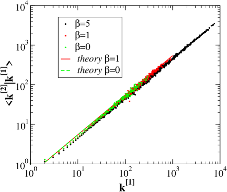
Figure 2: The average degree in layer 2 conditioned on the degree in layer 1, $\left\langle{k^{[2]}|k^{[1]}}\right\rangle$ is shown and compared with the mean-field theoretical expectations finding very good agreement. The data is shown for networks of $N=10^{4}$ nodes, energy distribution $g(\epsilon)=(1+\theta)\epsilon^{\theta}$ with $\theta=0.5$, $\alpha=0.3$ and $\beta=0,1,5$. The curves are averaged over $100$ multiplex networks realizations.

III.3 Bose-Einstein condensation in the supersymmetric multiplex network

The Bianconi-Barabási model Bose describing a growing scale-free networks that can mapped to a Bose-Einstein gas, displays the Bose-Einstein condensation in complex networks. This condensation transition is a structural phase transition occurring in the network when the mapped Bose gas is in the the Bose-Einstein condensation phase. Below this phase transition, in the network, one node grabs a finite fraction of the links and non trivial non-equilibrium process determine the network evolution.

A similar phenomenon occurs also in the supersymmetric multiplex model, where the condensation occurs simultaneously on the two replicas of the same node. In this model the condensation phase transition occurs at $\beta=\beta_{c}$ for which $\mu_{B}=0$. Therefore the equations determining the condensation phase transition are

$$\left\{\begin{array}[]{l}I_{B}=\int d\epsilon g(\epsilon)\frac{1}{e^{\beta_{c}\epsilon}-1}=G^{B},\\ I_{F}=\int d\epsilon g(\epsilon)\frac{1}{e^{\beta_{c}(\epsilon-\mu_{F})}+1}=G^{F},\\ \mu_{B}=0.\end{array}\right.$$ (51)

Below this phase transition a single node grabs a finite fraction of all the links in both layers. This condensation can possibly occur at low enough temperatures $T=1/\beta$ only if the integral $I_{B}(\mu_{B}=0)$ converges. Therefore, as in the classical Bose-Einstein condensation a necessary condition for this condensation to occur is that $g(\epsilon)\to 0$ as $\epsilon\to 0$.

Since the condensation occurs in the same node in the two layers, we observe that below the condensation transition the two layers develop another type of correlation. In fact we observe that the total overlap of the links in the two layers becomes significant below the condensation transition. The total overlap ${\cal O}^{[1,2]}$ of the links between two layers (in this case layer 1 and layer 2)PRE ; Note is defined as

$${\cal O}^{[1,2]}=\sum_{i<j}a_{ij}^{[1]}a_{ij}^{[2]},$$ (52)

where $a_{ij}^{[1]}$ and $a_{ij}^{[2]}$ are the matrix elements of the adjacency matrix of layer 1 and layer 2 respectively. In Figure 3 we plot the fraction of the links linked to the most connected node in layer 1 and in layer 2. The absence of finite size effects below the condensation phase transition shows that in the supersymmetric multiplex there is one node that grabs a finite fraction of all the links. Moreover, in Figure 3 we plot also the total overlap ${\cal O}^{[1,2]}$of the links, showing that below the condensation transition the total overlap becomes significant.

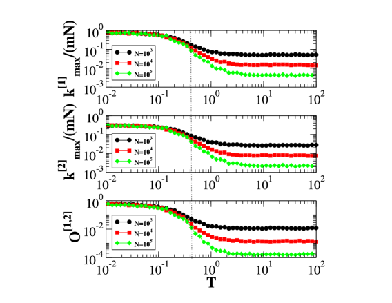
Figure 3: The fraction of links $k^{[1]}_{max}/(mN)$ and $k^{[2]}_{max}/(mN)$ linked to the most connected node in layer 1 and in layer 2 are shown together with the total overlap of the links ${\cal O}^{[1,2]}$ versus $T=1/\beta$.The data is shown for networks of $N=10^{3},10^{4},10^{5}$ nodes with energy distribution $g(\epsilon)=(1+\theta)\epsilon^{\theta}$ and $\theta=0.5$, $\alpha=0.3$. The curves are averaged over $100$ multiplex networks realizations for $N=10^{3}$ and $N=10^{4}$, and over $30$ multiplex network realization for $N=10^{5}$.

IV Entropy rate of the supersymmetric multiplex network

Given the initial condition, the supersymmetric multiplex evolution up to time $t$ is fully determined by the sequence of symbols $X=\{\sigma_{l}^{[1]},i^{[1]}_{l},\sigma^{[2]}_{l},i_{l}^{[2]}\}_{l=1,2,\ldots mt}$. Therefore, similarly to what happens for growing network models Entropyrate , it is possible to define an entropy rate of the growing supersymmetric multiplex network. This entropy rate $H(X)$ can be useful for example if aim at compressing the network, as we could aim at extending the Shannon’s noiseless coding theorem Quantuminformation to the sequence $X=\{\sigma_{l}^{[1]},i^{[1]}_{l},\sigma^{[2]}_{l},i_{l}^{[2]}\}_{l=1,2,\ldots mt}$ encoding the full network evolution. The entropy rate of the supersymmetric multiplex network model when in the supersymmetric multiplex we have already observed $l-1$ network changes, is given by

$$H(X) = -\sum_{{\bf x}_{l}}P({\bf x}_{l}|\{{\bf x}_{\ell}\}_{\ell=1,\ldots,l-1})$$ (53)

$$\times\log P({\bf x}_{l}|\{{\bf x}_{\ell}\}_{\ell=1,\ldots,l-1}),$$

where ${\bf x}_{l}=\{\sigma_{l}^{[1]},i^{[1]}_{l},\sigma^{[2]}_{l},i_{l}^{[2]}\}$. We note here that the entropy rate of the supersymmetric multiplex, as the entropy rate of growing networks has a very characteristic feature, i.e. contains a leading term of order of $\log(t)$. Therefore it does not converge in the thermodynamic limit $t\to\infty$. This is due to the fact that the attachment probability in these networks are non-local. This occurs also in the growth of other networks Entropyrate such as random trees, where each new node is attached to a random node of the network with probability $1/t$, where $t$ is the number of nodes in the network. In fact it is easy to see that also for this basic, non-local model we have

$$H(X)=\log(t).$$ (54)

V The entanglement entropies of the layers of the supersymmetric multiplex network

In order to evaluate the complexity of a single layer, recently new attention has been devoted to quantum information measures Vonneuman ; Garnerone ; Jesus2 . Already the von Neumann entropy Vonneuman of single networks has been extended to multilayer networks in Ref. Math . Here we propose to consider the entanglement entropies of the layers of the supersymmetric multiplex network as a generalization of the quantum entropy proposed in ¡ref. Garnerone . Following Garnerone here we perform a mapping between the layers of the supersymmetric multiplex network with $M=2$ and two bipartite quantum states. In particular we will consider the states $\left|{A^{[1]}}\right\rangle,\left|{A^{[2]}}\right\rangle\in{\cal H}_{a}\otimes{\cal H}_{b}$ with ${\cal H}_{a}\simeq{\cal H}_{b}\simeq\mathbb{C}^{N}$, given by

$$\left|{A^{[1]}}\right\rangle = \frac{1}{\parallel A^{[1]}\parallel}_{F}\sum_{i,j}e^{-\beta\epsilon_{i}/2}a^{[1]}_{ij}\left|{i}\right\rangle\left|{j}\right\rangle$$

$$\left|{A^{[2]}}\right\rangle = \frac{1}{\parallel A^{[2]}\parallel}_{F}\sum_{i,j}e^{-\beta\epsilon_{i}/2}a^{[2]}_{ij}\left|{i}\right\rangle\left|{j}\right\rangle$$ (55)

where ${\bf a^{[1]}}$ is the adjacency matrix of the first layer of the supersymmetric multiplex network, ${\bf a^{[2]}}$ is the adjacency matrix of the second layer of the supersymmetric multiplex network. Moreover, $\parallel A\parallel=\sqrt{\mbox{Tr}{\bf A}^{{\dagger}}{\bf A}}$ denotes the Frobenious norm of the matrix ${\bf A}$ and the matrix elements $(i,j)$ of the matrices ${\bf A^{[1]}}$ and ${\bf A^{[2]}}$ are given respectively by $A^{[1]}_{ij}=e^{-\beta\epsilon_{i}/2}a^{[1]}_{ij}$ and $A^{[2]}_{ij}=e^{-\beta\epsilon_{i}/2}a^{[2]}_{ij}$. Using the terminology of Garnerone we will refer to $\left|{A^{[1]}}\right\rangle$ and $\left|{A^{[2]}}\right\rangle$ as pure network states.

In order to characterize the complexity of the layers we propose to evaluate the entanglement entropy of the pure network states $\left|{A^{[1]}}\right\rangle$ and $\left|{A^{[2]}}\right\rangle$. Therefore we define the reduced density matrices $\rho^{[1]},\rho^{[2]}$ given by

$$\rho^{[1]} = \mbox{Tr}_{b}\left|{A^{[1]}}\right\rangle\langle A^{[1]}|,$$

$$\rho^{[2]} = \mbox{Tr}_{b}\left|{A^{[2]}}\right\rangle\langle A^{[2]}|$$ (56)

and we calculate the entanglement entropy $S^{[1]}$ and $S^{[2]}$ given by

$$S^{[1]} = -\mbox{Tr}_{a}\rho^{[1]}\log\rho^{[1]},$$

$$S^{[2]} = -\mbox{Tr}_{a}\rho^{[2]}\log\rho^{[2]}.$$ (57)

Using the explicit expression for the reduced density matrices in terms of the degree of the nodes in the different layers $\rho^{[1]}$ and $\rho^{[2]}$, i.e.

$$\rho^{[1]} = \sum_{i}\frac{e^{-\beta\epsilon_{i}}k_{i}^{[1]}}{\sum_{j}e^{-\beta\epsilon_{j}}k_{j}^{[1]}}\left|{i}\right\rangle\langle i|$$

$$\rho^{[2]} = \sum_{i}\frac{e^{-\beta\epsilon_{i}}k_{i}^{[2]}}{\sum_{j}e^{-\beta\epsilon_{j}}k_{j}^{[2]}}\left|{i}\right\rangle\langle i|$$ (58)

we found that the entropies $S^{[1]}$ and $S^{[2]}$ are given by

$$S^{[1]} = -\sum_{i}\frac{e^{-\beta\epsilon_{i}}k_{i}^{[1]}}{\sum_{j}e^{-\beta\epsilon_{j}}k_{j}^{[1]}}\log\left(\frac{e^{-\beta\epsilon_{i}}k_{i}^{[1]}}{\sum_{j}e^{-\beta\epsilon_{j}}k_{j}^{[1]}}\right),$$

$$S^{[2]} = -\sum_{i}\frac{e^{-\beta\epsilon_{i}}k_{i}^{[2]}}{\sum_{j}e^{-\beta\epsilon_{j}}k_{j}^{[2]}}\log\left(\frac{e^{-\beta\epsilon_{i}}k_{i}^{[2]}}{\sum_{j}e^{-\beta\epsilon_{j}}k_{j}^{[2]}}\right).$$ (59)

Moreover, in the asymptotic limit $t\gg 1$ we can evaluate the entropy using the asymptotic relations given by Eqs. $(\ref{asymptotics})$. We found that

$$E^{[1]}-TS^{[1]}+T\log(mc_{1}t)=F^{[1]}$$

$$E^{[2]}-TS^{[2]}+T\log(mc_{2}t)=F^{[2]}$$ (60)

where

$$E^{[\nu]} = \langle{\epsilon}\rangle_{\nu}$$

$$F^{[\nu]} = -T\langle{\log k^{[\nu]}}\rangle_{\nu}$$ (61)

with $\nu=1,2$ and

$$\left\langle{f}\right\rangle_{\nu}=\sum_{i}\frac{e^{-\beta\epsilon_{i}}k_{i}^{[\nu]}}{\sum_{j}e^{-\beta\epsilon_{j}}k_{j}^{[\nu]}}f_{i}$$ (62)

Finally by using the mean-field solution of the model we can evaluate the energies $E^{[1]},E^{[2]}$, and the free energies $F^{[1]},F^{[2]}$, as long as the supersymmetric multiplex is not in the condensed phase and $\alpha<0.5$. If we define $E_{B}$ and $E_{F}$ respectively as the average energies calculated over the Bose and Fermi distributions with “chemical potentials” $\mu_{B}$ and $\mu_{F}$, i.e.

$$E_{B}=\int d\epsilon g(\epsilon)\frac{\epsilon}{e^{\beta(\epsilon-\mu_{B})}-1}$$

$$E_{F}=\int d\epsilon g(\epsilon)\frac{\epsilon}{e^{\beta(\epsilon-\mu_{F})}+1}$$ (63)

we have, in the mean-field approximation,

$$\left(\begin{array}[]{c}E^{[1]}\\ E^{[2]}\end{array}\right)={\bf V}\left(\begin{array}[]{c}E_{B}\\ E_{F}\end{array}\right).$$ (66)

with

$${\bf V} = \left(\begin{array}[]{cc}\frac{1}{mc_{1}}d^{+}u_{1}^{+}\lambda^{+}&-\frac{1}{mc_{1}}d^{-}u_{1}^{-}\lambda^{-}\\ \frac{1}{mc_{2}}d^{+}u_{2}^{+}\lambda^{+}&-\frac{1}{mc_{2}}d^{-}u_{2}^{-}\lambda^{-}\end{array}\right).$$ (68)

Similarly also the “free energies” $F^{[1]}$ and $F^{[2]}$ can be estimated using the mean-field solution of the model.

VI Relation between the entanglement entropies of the supersymmetric multiplex and its entropy rate

We note here a surprising result. In fact the entanglement entropies $S^{[1]}$ and $S^{[2]}$ have a immediate classical meaning because they can be linked to the entropy rate of the network evolution. In fact, by calculating explicitly the entropy rate of the supersymmetric multiplex, defined in Eq. $(\ref{er})$, we get

$$H(X)=S^{[1]}+S^{[2]}+2h(\alpha)$$ (69)

where $h(\alpha)$ is given by

$$h(\alpha)=-\alpha\log(\alpha)-(1-\alpha)\log(1-\alpha).$$ (70)

Therefore, the entanglement entropies of the supersymmetric multiplex network are related to the entropy rate of the supersymmetric multiplex, which is described by a classical non-equilibrium process. The relation between the entropy rate $H(X)$ and the entanglement entropies $S^{[1]}$ and $S^{[2]}$ remains valid for every value of $\alpha\in[0,1)$ and also below the condensation phase transition. Nevertheless, the scaling of the entanglement entropies with the system size changes below the condensation phase transition.

VII Conclusions

In conclusion here we have investigated the properties of the supersymmetric multiplex network model in which nodes have intrinsic fitness and the evolution describes both the addition of new links according to the generalized preferential attachment, and rewring of the links. The resulting multiplex network has scale-free layers and develops interesting degree-degree correlations. The supersymmetric multiplex model can be fully characterized by coupled quantum Bose-Einstein and Fermi-Dirac statistics. In fact the dynamic rules of the supersymmetric multiplex networks evolution exploit the symmetries of the multilayer structure and, as a consequence of this, the multiplex network evolution is not determined exclusively by the Bose-Einstein statistics or by the Fermi-Dirac statistics, but is determined by Bose-Einstein and Fermi-Dirac statistics with coupled “chemical potentials” $\mu_{B}$ and $\mu_{F}$. The resulting supersymmetric multiplex network can undergo a Bose-Einstein condensation of the links in which one node acquires a finite fraction of the links in all the layers, and simultaneously every pair of layers develops a significant overlap of the links. Moreover, an interesting relation has been shown to exists between the entanglement entropies of the layers in the supersymmetric multiplex network, measuring the complexity of these layers with quantum information theory tools, and the entropy rate of the classical supersymmetric multiplex network. In conclusion, in this work the evolution of supersymmetric multiplex networks with fitness of the nodes is characterized. The complexity of the supersymmetric multiplex networks, and its underlying symmetries have been shown to be related to quantum statistics. In fact in multilayer networks there are additional symmetries that are not present in undirected single networks. These symmetries allow for an evolution determined simultaneously by Bose-Einstein and Fermi-Dirac statistics. Moreover, interesting results relate the complexity of these structures measured by quantum information theory tools and their non equilibrium classical dynamics determined by their entropy rate.

Appendix A Supersymmetric multiplex networks with $M$ layers

We consider here the extension of the supersymmetric multiplex model defined in the main text for a multiplex network of $M=2$ layers to the case in which the multiplex is formed by a generic number $M$ of layers. We suppose that the layers can be distinguished in two groups: a first group of $M_{1}$ layers $\xi=1,2\ldots,M_{1}$ in which the dynamics only include addition of new links, a second group of $M_{2}$ layers $\psi=M_{1}+1,M_{1}+2,\ldots,M_{1}+M_{2}$ in which the network dynamics includes both addition of new links are rewiring of the links. Clearly we must have $M_{1}+M_{2}=M$. In particular we consider the following model. We start at $t=0$ from a small set of nodes $N_{0}$ connected in each of the $M$ layers. Each node $i$ of the network has degrees $k^{[\xi]}_{i}$, in the layers $\xi=1,2,\ldots,M_{1}$ and degrees $k^{[\psi]}_{i}$ in the layers $\psi=M_{1}+1,M_{1}+2\ldots,M_{1}+M_{2}$. Moreover each node has an energy $\epsilon_{i}$ drawn from a $g(\epsilon)$ distribution and a fitness given by $\eta_{i}=e^{-\beta\epsilon_{i}}$. At each time $t$ we add a node to the multiplex network, each node has $M$ replicas nodes, one on each layer and each replica node is initially attached to $m$ existing nodes in the same layer. In the following we will indicate with $l$ the number of network changes, i.e. links additions or link rewirings, occurring in each layer starting from time $t=1$. After time $t$ we will have $l=mt$. For each network change in a layer $\xi$ we follow the subsequent procedure:

• We extract a number $\sigma^{[\xi]}_{l}=\phi$ with $\phi=1,2,\ldots,M$. The event $\sigma^{[1]}_{l}=\xi^{\prime}$ with $\xi^{\prime}=1,2,\ldots,M_{1}$ occurs with probability $p^{[\xi]}(\xi^{\prime})=\alpha/M_{1}$ while the event $\sigma_{l}^{[\xi]}=\psi^{\prime}$ with $\psi^{\prime}=M_{1}+1,\ldots,M_{1}+M_{2}$ occurs with probability $p^{[\xi]}(\psi^{\prime})=(1-\alpha)/M_{2}$.

• If $\sigma^{[\xi]}_{l}=\xi^{\prime}$, the new node is attached in layer $\xi$ to a node $i^{[\xi]}_{l}$ chosen with probability

  $$\Pi^{[\xi,\xi^{\prime}]}\left(i_{l}^{[\xi]}=i\right)=\frac{e^{-\beta\epsilon_{i}}k_{i}^{[\xi^{\prime}]}}{\sum_{j}e^{-\beta\epsilon_{j}}k_{j}^{[\xi^{\prime}]}},$$ (71)

  i.e. it will be attached preferentially to nodes with low energy and high degree in layer $\xi^{\prime}$, according to a generalized preferential attachment driven by layer $\xi^{\prime}$. Instead, if $\sigma^{[1]}_{l}=\psi^{\prime}$ the new node is attached in layer $\xi$ to a node $i^{[\xi]}_{l}$ chosen with probability

  $$\Pi^{[\xi,\psi^{\prime}]}\left(i_{l}^{[\xi]}=i\right)=\frac{e^{-\beta\epsilon_{i}}k_{i}^{[\psi^{\prime}]}}{\sum_{j}e^{-\beta\epsilon_{j}}k_{j}^{[\psi^{\prime}]}}.$$ (72)

  In other words the new node will be attached preferentially to nodes with low energy and high degree in layer $\psi^{\prime}$, according to a generalized preferential attachment.

For each network change in layer $\psi$ we follow the subsequent procedure:

• We extract a number $\sigma^{[\psi]}_{l}=\phi$ with $\phi=1,2\ldots,M$. The event $\sigma^{[\psi]}_{l}=\xi^{\prime}$ with $\xi^{\prime}=1,2,\ldots,M_{1}$ occurs with probability $p^{[\psi]}(\xi^{\prime})=(1-\alpha)/M_{1}$ while the event $\sigma_{l}^{[\psi]}=\psi^{\prime}$ with $\psi=M_{1}+1,\ldots,M_{1}+M_{2}$ occurs with probability $p^{[\psi]}(\psi^{\prime})=\alpha/M_{2}$.

• If $\sigma^{[\psi]}_{l}=\xi^{\prime}$ the new node will be attached, in layer $\psi$, to a node $i_{l}^{[\psi]}$ chosen with probability

  $$\Pi^{[\psi,\xi^{\prime}]}\left(i_{l}^{[\psi]}=i\right)=\frac{e^{-\beta\epsilon_{i}}k_{i}^{[\xi^{\prime}]}}{\sum_{j}e^{-\beta\epsilon_{j}}k_{j}^{[\xi^{\prime}]}}.$$ (73)

  Instead, if $\sigma^{[\psi]}_{l}=\psi^{\prime}$ a random link of a node $i^{[\psi]}_{l}$ chosen with probability

  $$\Pi^{[\psi,\psi^{\prime}]}\left(i_{l}^{[\psi]}=i\right)=\frac{e^{-\beta\epsilon_{i}}k_{i}^{[\psi^{\prime}]}}{\sum_{j}e^{-\beta\epsilon_{j}}k_{j}^{[\psi^{\prime}]}}$$ (74)

  is rewired, i.e. it is detached from node $i_{l}^{[\psi]}$ and attached to the new node of the network.

Therefore the network is determined by the sequence of the values $\{\sigma^{[\xi]}_{l},i_{l}^{[\xi]}\sigma^{[\psi]}_{l},i_{l}^{[\psi]}\}_{\xi=1,2\ldots,M_{1},\psi^{\prime}=M_{1}+1\ldots,M_{1}+M_{2}}$ that fully determines the evolution of the multiplex network given the initial condition.

The mean-field treatment of the model can be performed exactly has in the case of the supersymmetric multiplex networks formed by $M=2$ layers. In fact the mean field equations for the degree in each layer read

$$\frac{dk_{i}^{[\xi]}}{dt} = me^{-\beta\epsilon_{i}}\left[\alpha\frac{1}{M_{1}}\sum_{\xi^{\prime}}\frac{1}{\sum_{j}e^{-\beta\epsilon_{j}}k_{j}^{[\xi^{\prime}]}}k_{i}^{[\xi^{\prime}]}\right.$$

$$\left.+(1-\alpha)\frac{1}{M_{2}}\sum_{\psi^{\prime}}\frac{1}{\sum_{j}e^{-\beta\epsilon_{j}}k_{j}^{[\psi^{\prime}]}}k_{i}^{[\psi^{\prime}]}\right],$$

$$\frac{dk_{i}^{[\psi]}}{dt} = me^{-\beta\epsilon_{i}}\left[\frac{(1-\alpha)}{M_{1}}\sum_{\xi^{\prime}}\frac{1}{\sum_{j}e^{-\beta\epsilon_{j}}k_{j}^{[\xi^{\prime}]}}k_{i}^{[\xi^{\prime}]}\right.$$ (75)

$$\left.-\frac{\alpha}{M_{2}}\sum_{\psi^{\prime}}\frac{1}{\sum_{j}e^{-\beta\epsilon_{j}}k_{j}^{[\psi^{\prime}]}}k_{i}^{[\psi^{\prime}]}\right].$$

We note that in the mean field equation the degree of the nodes in the layer $\xi=1,2\ldots,M_{1}$ are all the same, while the degree of the nodes in the layers $\psi=M_{1}+1,\ldots,M_{1}+M_{2}$ are also all the same, therefore we can write the mean-field equation for the average degree in the first group of layers $k_{i}^{[\xi]}=\kappa_{i}^{[1]}\ \forall\xi=1,2\ldots,M_{1}$ and the average degree in the second group of layers $k_{i}^{[\psi]}=\kappa_{i}^{[2]}\ \forall\psi=M_{1}+1,\ldots,M_{1}+M_{2}$. We have in particular

$$\frac{d\kappa_{i}^{[1]}}{dt}=me^{-\beta\epsilon_{i}}\left[\frac{\alpha}{\sum_{j}e^{-\beta\epsilon_{j}}\kappa_{j}^{[1]}}\kappa_{i}^{[1]}+\frac{(1-\alpha)}{\sum_{j}e^{-\beta\epsilon_{j}}\kappa_{j}^{[2]}}\kappa_{i}^{[2]}\right],$$

$$\frac{d\kappa_{i}^{[2]}}{dt}=me^{-\beta\epsilon_{i}}\left[\frac{(1-\alpha)}{\sum_{j}e^{-\beta\epsilon_{j}}\kappa_{j}^{[1]}}\kappa_{i}^{[1]}-\frac{\alpha}{\sum_{j}e^{-\beta\epsilon_{j}}\kappa_{j}^{[2]}}\kappa_{i}^{[2]}\right].$$ (76)

These equations read completely equivalent to the mean-field equations Eqs. $(\ref{mf0})$ for the supersymmetric multiplex network of $M=2$ layers. Moreover it is straightforward to generalize the definition of the entanglement entropies of each layer, introduced in the main text for the $M=2$ case, for this general case. It is immediate to see that also in this general case the sum of the entanglement entropies of each layer of the supersymmetric multiplex are linearly related with its entropy rate. This last result is independent on the validity of the mean-field approach and is a fundamental characteristic of this model.

References

• (1) R. Albert and A.-L. Barabasi, Reviews of Modern Physics 74, 47 (2002).
• (2) M. E. J. Newman, SIAM Review 45, 167-256 (2003).
• (3) S. Boccaletti, V. Latora, Y. Moreno, M. Chavez and D.-U. Hwang, Physics Reports 424, 175 - 308 (2006).
• (4) S. Perseguers, M. Lewenstein, A. Acín, J. I. Cirac, Nature Physics 6, 539 (2010).
• (5) M. Cuquet and J. Calsamiglia, Phys. Rev. Lett. 103, 240503 (2009).
• (6) S. Sachdev Quantum Phase transitions (Cambridge University Press, Cambridge, 2011).
• (7) G. Bianconi, Phys. Rev. E 85, 061113 (2012).
• (8) A. Halu, L. Ferretti, A. Vezzani and G. Bianconi, EPL 99 18001 (2012).
• (9) A. Halu, S. Garnerone, A. Vezzani, and G. Bianconi, Phys. Rev. E 87, 022104 (2013).
• (10) M.A. Nielsen, I.L. Chuang, Quantum Information and Quantum Computation (Cambridge University Press, Cambridge, 2010).
• (11) D. Krioukov, M. Kitsak, R. S. Sinkovits, D. Rideout, D. Meyer, M. Boguñá, Scientific Reports 2, 793 (2012).
• (12) J. Ambjorn, J. Jurkiewicz, and R. Loll, Phys. Rev. D 72, 064014 (2005).
• (13) C. Rovelli, Quantum Gravity (Cambridge University Press, Cambridge, 2004).
• (14) G. Chirco, H. M. Haggard, A. Riello, C. Rovelli, arXiv:1401.5262 (2014).
• (15) G. Bianconi, A.-L. Barabási, EPL 54, 436 (2001).
• (16) G. Bianconi and A.-L. Barabási, Phys. Rev. Lett. 86, 5632 (2001)
• (17) G. Bianconi, Phys. Rev. E 66, 036116 (2002).
• (18) G. Bianconi, Phys. Rev. E 66, 056123 (2002).
• (19) D. Garlaschelli, M. I. Loffredo, Phys. Rev. Lett. 102, 038701 (2009).
• (20) D. Krioukov, F. Papadopoulos, M. Kitsak, A. Vahdat, and M. Boguñá, Phys. Rev. E 82, 036106 (2010).
• (21) M. Boguñá, D. Krioukov, K. C. Claffy, Nature Physics 5, 74 (2009).
• (22) K. Anand, G. Bianconi, S. Severini, Phys. Rev. E 83, 036109 (2011).
• (23) S. Garnerone, P. Giorda, P. Zanardi, New J. Phys. 14, 013011 (2012).
• (24) A. Cardillo, F. Galve, D. Zueco, and J. Gómez-Gardeñes, Phys. Rev. A 87, 052312 (2013).
• (25) S. Garnerone, P. Zanardi, and D. A. Lidar, Phys. Rev. Lett. 108, 230506 (2012).
• (26) E. Sanchez-Burillo,J. Duch,J. Gomez-Gardeñes,D. Zueco, Scientific Reports 2,605 (2012).
• (27) N. Perra, V. Zlatić, A. Chessa, C. Conti, D. Donato and G. Caldarelli, EPL 88 48002 (2009).
• (28) M. Faccin, T. Johnson, J. Biamonte, S. Kais, and P. Migdal, Phys. Rev. X 3, 041007 (2013).
• (29) Z. Zimborás, M. Faccin, Z. Kádár, J. D. Whitfield, B. P. Lanyon , J. Biamonte, Scientific Reports 3, 2361 (2013).
• (30) S. Boccaletti, G. Bianconi, R. Criado, C.I. del Genio, J. Gómez-Gardeñes, M. Romance, I. Sendiña-Nadal, Z. Wang, M. Zanin, Physics Reports 544, 1 (2014).
• (31) M. Kivelä, A. Arenas, M. Barthelemy, J. P. Gleeson, Y. Moreno, M. A. Porter, Jour. Complex Networks 2, 203 (2014).
• (32) K. Zhao, A. Halu, S. Severini, and G. Bianconi Phys. Rev. E 84, 066113 (2011).
• (33) E. Bullmore, O. Sporns, Nature Reviews Neuroscience 10, 186-198 (2009).
• (34) S. D. Reis, Y. Hu, A. Babino, J. S. Andrade Jr., S. Canals, M. Sigman, H. A. Makse, Nature Physics 10, 762(2014).
• (35) G. Bianconi, Nature Physics 10, 712 (2014).
• (36) P.J. Mucha, T. Richardson, K. Macon,M.A. Porter, J.P. Onnela, Science, 328, 876 (2010).
• (37) G. Bianconi, Phys. Rev. E 87, 062806 (2013).
• (38) K. M. Lee, J. Y. Kim, W.K. Cho, K. I. Goh and I. M. Kim, New Journal of Physics 14 033027 (2012).
• (39) F. Battiston, V. Nicosia, V. Latora, V. Physical Review E, 89, 032804 (2014).
• (40) M. De Domenico, A. Solé-Ribalta, E. Cozzo, M. Kivelä, Y. Moreno, M. A. Porter, S. Gómez, A. Arenas, Phys. Rev. X 3, 041022 (2013).
• (41) V. Nicosia, G. Bianconi, V. Latora, and M. Barthelemy, Phys. Rev. Lett. 111, 058701 (2013).
• (42) J. Y. Kim and K.-I. Goh, Phys. Rev. Lett. 111, 058702 (2013).
• (43) V. Nicosia, G. Bianconi, V. Latora, M. Barthelemy, Phys. Rev. E 90, 042807 (2014).
• (44) A.-L. Barabási and R. Albert, Science, 286, 509-512 (1999).
• (45) S.N. Dorogovtsev and J. F.F. Mendes Evolution of networks: From biological nets to the Internet and WWW (Oxford University Press,Oxford, 2003).
• (46) This definition is valid for unweighted layers, for a generalization to weighted layers see Weighted .
• (47) G. Menichetti, P. Panzarasa, R.J. Mondragon, G. Bianconi, PloS one 9 e97857 (2014).