Accelerated Matrix Element Method with Parallel Computing

Abstract

The matrix element method utilizes ab initio calculations of probability densities as powerful discriminants for processes of interest in experimental particle physics. The method has already been used successfully at previous and current collider experiments. However, the computational complexity of this method for final states with many particles and degrees of freedom sets it at a disadvantage compared to supervised classification methods such as decision trees, $k$ nearest-neighbour, or neural networks. This note presents a concrete implementation of the matrix element technique using graphics processing units. Due to the intrinsic parallelizability of multidimensional integration, dramatic speedups can be readily achieved, which makes the matrix element technique viable for general usage at collider experiments.

1 Introduction

The matrix element method (MEM) in experimental particle physics is a unique analysis technique for characterizing collision events. When used to define a discriminant for event classification, it differs from supervised multivariate methods such as neural networks, decision trees, $k$-NN, and support vector machines in that it employs unsupervised ab initio calculations of the probability density $P_{i}$ that an observed collision event with a particular final state arises from $2\to N$ scattering process $i$. Furthermore, the strong connection of this technique to the underlying particle physics theory provides key benefits compared to more generic methods:

1. the probability density $P_{i}$ directly depends on the physical parameters of interest;

2. it provides a most powerful test statistic for discriminating between alternative hypotheses, namely $P_{i}/P_{j}$ for hypotheses $i$ and $j$, by the Neyman-Pearson lemma;

3. it avoids tuning on unphysical parameters for analysis optimization;

4. it requires no training, thereby mitigating dependence on large samples of simulated events.

The MEM was first studied in [1] and was heavily utilized by experiments at the Tevatron for $W$ helicity [2] and top mass [3, 4] measurements, and in the observation of single top production [5], for example. It has also been used in Higgs searches at the Tevatron [6] and at the Large Hadron Collider (LHC) by both CMS [7] and ATLAS [8] collaborations. Good introductions to the MEM in the context of top mass measurements can be found in [9, 10]. The MEM has also been extended in a general framework known as MadWeight [11].

The MEM derives its name from the evaluation of $P_{i}$:

$$P_{i}=\frac{1}{\sigma_{i}}\displaystyle\sum_{\textrm{flavor}}\int_{V_{n}}\mathcal{M}^{2}_{i}({\bf Y})\,\frac{f_{1}(x_{1},Q^{2})\,f_{2}(x_{2},Q^{2})}{|\vec{q}_{1}|\cdot|\vec{q}_{2}|}\,d\Phi_{n}(q_{1}+q_{2};y_{1},..,y_{n}),$$ (1)

where $\mathcal{M}_{i}$ is the the Lorentz invariant matrix element for the $2\to n$ process $i$, ${\bf Y}$ is shorthand notation for all the momenta $\vec{y}$ of each of the $n$ initial and final state particles, $f_{1}$ and $f_{2}$ are the parton distribution functions (PDF’s) for the colliding partons, $\sigma$ is the overall normalization (cross-section), and

$$d\Phi_{n}(q_{1}+q_{2};y_{1},..,y_{n})=(2\pi)^{4}\delta^{4}(q_{1}+q_{2}-\sum_{i=1}^{n}y_{i})\prod_{i=1}^{n}\frac{d^{3}y_{i}}{(2\pi)^{3}2E_{i}}$$ (2)

is the n-body phase space term. The momenta of the colliding partons are given by $q_{1}$ and $q_{2}$, and the fractions of the proton beam energy are $x_{1}$ and $x_{2}$, respectively. The sum in Equation (1) indicates a sum over all relevant flavor combinations for the colliding partons.

The association of the partonic momenta ${\bf Y}$ with the measured momenta ${\bf X}$ is given by a transfer function (TF), $T(\vec{x};\vec{y})$ for each final state particle. The TF provides the conditional probability density function for measuring $\vec{x}$ given parton momentum $\vec{y}$. Thus,

$$\hat{p}_{i}=\int P_{i}\,T({\bf X};{\bf Y})\;d{\bf Y},$$ (3)

is the MEM probability density for an observed event to arise from process $i$ assuming the parton $\to$ observable evolution provided by the TF’s. For well-measured objects like photons, muons and electrons, the TF is typically taken to be a $\delta$-function. For unobserved particles such as neutrinos, the TF is a uniform distribution. The TF for jet energies is often modeled with a double Gaussian function, which accounts for detector response (Gaussian core) and also for parton fragmentation outside of the jet definition (non-Gaussian tail). To reduce the number of integration dimensions, the jet directions are assumed to be well-modeled so that $T(\theta_{x},\phi_{x};\theta_{y},\phi_{y})=\delta(\theta^{x}-\theta^{y})\delta(\phi^{x}-\phi^{y})$.

Despite the advantages provided by the MEM enumerated above, an important obstacle to overcome is the computational overhead in evaluating $\geq 1$ multi-dimensional integrals for each collision event. For complex final states with many degrees of freedom (eg., many particles with broad measurement resolution, or unobserved particles), the time needed to evaluate $\hat{p}_{i}$ can exceed many minutes. In realistic use cases, the calculations must be performed multiple times for each event, such as in the context of a parameter estimation analysis where $\hat{p}_{i}$ is maximized with respect to a parameter of interest, or for samples of simulated events used to study systematic biases with varied detector calibrations or theoretical parameters. For large samples of events, the computing time can be prohibitive, even with access to powerful computer clusters. Therefore, overcoming the computation hurdle is a relevant goal.

This paper presents an implementation of the MEM using graphics processing units (GPU’s). The notion of using GPU’s for evaluating matrix elements in a multidimensional phase space has been investigated previously [12], although not in the context of the MEM. In order to ascertain the improvements in computing time when utilizing GPU’s, the MEM was applied in the context of a simplified $t\bar{t}H(\to b\bar{b})$ search in LHC Run II. Studying the $t\bar{t}H$ process is important in its own right [13, 14, 15, 16, 17]. Due to the complexity of the final state for this process, it is also an interesting use case in which to study the feasibility of the MEM with the improvements from highly parellelized multi-dimensional integration.

The note is organized as follows: in Section 2, the applicability of GPU architectures to the computational problem at hand is briefly outlined. In Section 3 a simplified $t\bar{t}H$ analysis is presented, which will be used to benchmark the improved computational performance afforded by modern GPU’s. In Section 4 the specific implementation is outlined together with a summary of the results obtained from a number of GPU and CPU architectures. Further details of the codes are listed in A.

2 Parallelized Integrand Evaluation

For dimensions $\geq$ 3, evaluation of multidimensional integrals is typically only feasible using Monte Carlo methods. In these methods, the integrand

$$I=\int_{V_{m}}f(\vec{x})\;d\vec{x}$$ (4)

is approximated by a sum over randomly sampled points in the $m$-dimensional integration volume $V_{m}$

$$S_{N}\equiv V_{m}\,\underbrace{\frac{1}{N}\displaystyle\sum_{i=1}^{N}f(\vec{x}_{i})}_{\equiv\;\overline{f}},$$ (5)

which converges to $I$ by the law of large numbers. The residual error after evaluating $N$ points is determined by

$$\Delta S_{N}\approx\frac{V_{m}}{\sqrt{N}}\underbrace{\left(\frac{1}{N-1}\displaystyle\sum_{i=1}^{N}(f(\vec{x}_{i})-\overline{f})^{2}\right)}_{\equiv\;\sigma_{f}}.$$ (6)

This error estimate is not a strict upper bound, and there can be significant departures from it depending on the function $f(\vec{x})$. Modifications to the simplest Monte Carlo sampling employ stratified and importance sampling techniques to improve this error estimate, by ensuring that regions in which the function varies greatly are sampled more frequently. One such approach is given by the Vegas algorithm [18, 19]. For all such Monte Carlo integration algorithms, there is a trivial parallelization that can be achieved by evaluating the integrand $f(x_{i})$ at points $\{x_{i}\}_{i=1,..,N}$ simultaneously, since the evaluation of the integrand at each point $x_{i}$ is independent of all other points $\{x_{j}\}_{j\neq i}$.

This mode of parallel evaluation is known as data parallelism, which is achieved by concurrently applying the same set of instructions to each data element. In practice, evaluating the functions used in the MEM involves conditional branching, so that the integrand calculation at each $x_{i}$ does not follow an identical control flow. Nevertheless, it is instructive to proceed with the ansatz of strict data parallelism.

Data parallelism maps very well to the single instruction, multiple data (SIMD) architecture of graphics processing units (GPU’s). Modern GPU’s contain many individual compute units organized in thread units. Within each thread unit, all threads follow the same instruction sequence, and have access to a small shared memory cache in addition to the global GPU memory.

The advent of general purpose programming on GPU’s (GPGPU) has vastly increased the computing capability available on a single workstation, especially for data parallel calculations such as in the MEM. Two languages have gained traction for GPGPU, namely CUDA [20] (restricted to GPU’s manufactured by NVidia) and OpenCL [21]. Both languages are based on C/C++.

3 $t\bar{t}H(\to b\bar{b})$ Search

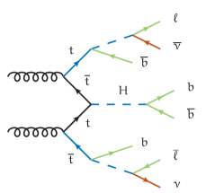
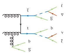
Figure 1: Representative Feynman diagrams for $t\bar{t}H(\to b\bar{b})$ production (left) and the irreducible $t\bar{t}b\bar{b}$ background (right).

The fact that the Higgs coupling to the top quark is $\approx$ 1 hints at a special role played by the top quark in electroweak symmetry breaking. Analysis of $t\bar{t}H(\to b\bar{b})$ production at the LHC can provide a powerful direct constraint on the fermionic (specifically, the top) couplings of the Higgs boson, with minimal model-dependence. The dominant backgrounds to this process, assuming at least one leptonic top decay, arise from the irreducible $t\bar{t}b\bar{b}$ background as well as the $t\bar{t}c\bar{c}$ and $t\bar{t}jj$ backgrounds via ‘fake’ $b$-tagged jets. The association of observed jets to the external lines of the leading order (LO) Feynman diagrams in Figure 1 also gives rise to a combinatoric dilution of the signal, since there is an increased probability that a random pair of $b$ partons in a $t\bar{t}b\bar{b}$ event will have $m_{bb\,^{\prime}}\approx m_{H}$. For the fully hadronic $t\bar{t}$ decay, there are 4! $\times$ 4! / 2= 288 combinations, assuming fully efficient $b$-tagging. This benchmark study is restricted to the dileptonic $t\bar{t}$ decay mode, to reduce the combinatoric and also the large $W$+jet(s) and QCD backgrounds.

For the dilepton channel, the observable signature of the final state is $b\bar{b}\ell\bar{\ell}$ + $\not{E}_{T}$, where $\not{E}_{T}=\vec{p}_{T}^{\nu}+\vec{p}_{T}^{\bar{\nu}}$. It is not possible to constrain the $z$ components of the neutrino momenta, and using transverse momentum balance removes only two of the remaining four degrees of freedom from the $x$ and $y$ components. Due to the broad resolution of the measured jet energy, there are also four degrees of freedom for the energy of the four $b$ quarks in the final state, so that the MEM evaluation implies an 8-dimensional integration:

$$\hat{p}_{i} = \frac{1}{\sigma_{i}}\displaystyle\sum_{\textrm{jet comb.}}\displaystyle\sum_{\textrm{flavor}}\int\mathcal{M}^{2}_{i}({\bf Y})\,\frac{f_{1}(x_{1},Q^{2})\,f_{2}(x_{2},Q^{2})}{|\vec{q}_{1}|\cdot|\vec{q}_{2}|}\;\Phi\cdot$$

$$\;\;\;\;\delta\left(p_{x}^{\nu}-\not{E}_{T}^{x}-p_{x}^{\bar{\nu}}\right)\,\delta\left(p_{y}^{\nu}-\not{E}_{T}^{y}-p_{y}^{\bar{\nu}}\right)\,d^{3}\vec{p}_{\nu}\,d^{3}\vec{p}_{\bar{\nu}}\prod_{j=1}^{N_{\textrm{jet}}=4}\textrm{T}\,(E^{\textrm{jet}}_{j};E_{j})\cdot(E_{j}^{2}\,\textrm{sin}\,\theta_{j})\,dE_{j},$$

where $\Phi=(2\pi)^{4}\delta^{4}(q_{1}+q_{2}-\sum_{i=1}^{n}p_{y}^{i})\prod_{i=1}^{n}\frac{1}{(2\pi)^{3}2E_{i}}$, and the integrals over the lepton momenta are removed by assuming infinitesimal measurement resolution. The outer sum is over all permutations of assigning measured jets to partons in the matrix element. A transformation to spherical coordinates has been performed $d^{3}\vec{p}\to p^{2}\,\textrm{sin}(\theta)\,dp\,d\theta\,d\phi$ for the jets, and $E$ is set to $|p|$.

The behaviour of the matrix element function $\mathcal{M}({\bf Y})$ is strongly influenced by whether or not the internal propagators are on shell. It is difficult for numerical integration algorithms to efficiently map out the locations in momentum space of the external lines for which the internal lines are on shell. Therefore, it is advantageous to transform integration over the neutrino momenta to integrals over $q^{2}$ (where $q$ is the four momentum) of the top quark and $W$ boson propagators, so that the poles in the integration volume are along simple hyperplanes. This leads to the following coupled equations:

$$\not{E}_{x} = p^{\nu}_{x}+p^{\bar{\nu}}_{x}$$

$$\not{E}_{y} = p^{\nu}_{y}+p^{\bar{\nu}}_{y}$$

$$q_{W^{+}}^{2} = (E_{\ell^{+}}+E_{\nu})^{2}-(p^{\ell^{+}}_{x}+p^{\nu}_{x})^{2}-(p^{\ell^{+}}_{y}+p^{\nu}_{y})^{2}-(p^{\ell^{+}}_{z}+p^{\nu}_{z})^{2}$$

$$q_{W^{-}}^{2} = (E_{\ell^{-}}+E_{\bar{\nu}})^{2}-(p^{\ell^{-}}_{x}+p^{\bar{\nu}_{x}})^{2}-(p^{\ell^{-}}_{y}+p^{\bar{\nu}_{y}})^{2}-(p^{\ell^{-}}_{z}+p^{\bar{\nu}_{z}})^{2}$$ (8)

$$q_{t}^{2} = (E_{b}+E_{\ell^{+}}+E_{\nu})^{2}-(p^{b}_{x}+p^{\ell^{+}}_{x}+p^{\nu}_{x})^{2}-$$

$$(p^{b}_{y}+p^{\ell^{+}}_{y}+p^{\nu}_{y})^{2}-(p^{b}_{z}+p^{\ell^{+}}_{z}+p^{\nu}_{z})^{2}$$

$$q_{\bar{t}}^{2} = (E_{\bar{b}}+E_{\ell^{-}}+E_{\bar{\nu}})^{2}-(p^{\bar{b}}_{x}+p^{\ell^{-}}_{x}+p^{\bar{\nu}}_{x})^{2}-$$

$$(p^{\bar{b}}_{y}+p^{\ell^{-}}_{y}+p^{\bar{\nu}}_{y})^{2}-(p^{\bar{b}}_{z}+p^{\ell^{-}}_{z}+p^{\bar{\nu}}_{z})^{2},$$

which have been solved analytically in [23]. For the $t\bar{t}H(\to b\bar{b})$ process, there is an additional very narrow resonance from the Higgs propagator. For the same reasoning as above, the following transformation of variables for $E_{1}$ and $E_{2}$ are employed, which are the energies of the $b$-quarks from the Higgs decay, respectively:

$$f = (E_{1}+E_{2})$$

$$m_{H}^{2} = (E_{1}+E_{2})^{2}-|\vec{p}_{1}|^{2}-|\vec{p}_{2}|^{2}-2\,|\vec{p}_{1}|\,|\vec{p}_{2}|\,\textrm{cos}\,\Delta\theta_{1,2},$$ (9)

where $|\vec{p}|=\sqrt{E^{2}-m^{2}}$. Figure 1 highlights the internal lines which are used in the integration.

4 Analysis and Results

The evaluation of the integrand in Equation (3) is broken into components for the matrix element $\mathcal{M}({\bf Y})$, the PDF’s, the TF’s and the phase space factor. Each of these components is evaluated within a single GPU “kernel” program for each phase space point. Code for evaluating $\mathcal{M}$ is generated using a plugin developed for MadGraph [24]. This plugin allows one to export code for an arbitrary $2\to N$ process from MadGraph to a format compatible with OpenCL, CUDA, and standard C++. This code is based on HELAS functions [25, 26]. Compilation for the various platforms is controlled with precompiler flags. Model parameters, PDF grids and phase space coordinates are loaded in memory and transferred to the device (GPU) whereafter the kernel is executed. The PDF’s are evaluated within the kernel using wrapper code that interfaces with LHAPDF [27] and with the CTEQ [28] standalone PDF library. The PDF data is queried from the external library and stored in $(x,Q^{2})$ grids for each parton flavor ($d,u,s,c,b$), which are passed to the kernel program. The PDF for an arbitrary point is evaluted using bilinear interpolation within the kernel. The precision of the interpolation is within 1% of the values directly queried from the PDF library. An event discriminant $D$ is constructed as

$$D=\textrm{log}_{10}\left(\frac{\hat{p}_{t\bar{t}H}}{\hat{p}_{t\bar{t}b\bar{b}}}\right)$$ (10)

and evaluated for a sample of signal ($t\bar{t}H$) and background ($t\bar{t}b\bar{b}$) events generated in MadGraph and interfaced with Pythia for the parton shower, [29] using the so-called Perugia tune [30]. Jets are reconstructed using the anti-$k_{T}$ algorithm described in [31] with width parameter $d=0.4$. Any jets overlapping with leptons within $d$ are vetoed, and $b$-tagging is performed by matching jets to the highest energy parton within $\Delta R=\sqrt{\Delta\eta^{2}+\Delta\phi^{2}}<d$. A transfer function is defined for $b$-jets by fitting the ratio of jet energy to the energy of the matched parton using a double Gaussian distribution, as shown in Figure 2.

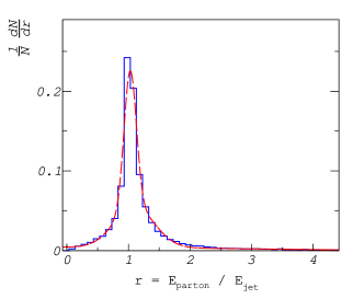
Figure 2: The ratio of parton energy to jet energy for jets reconstructed with the anti-$k_{T}$ algorithm and matched to partons within $\Delta R<0.4$. The fitted transfer function is also shown.

The analysis is performed at two levels, namely

1. parton level: using the parton momenta from MadGraph-generated events directly (by assuming $\delta$-function TF’s for all final state particles), and averaging over all permutations for the assignment of the $b$ partons in each event;

2. hadron level: using the outputs from Pythia and selecting events with four $b$-jets, averaging over all the permutations and integrating over the full 8-dimensional phase space as in Equation (3).

The convenient PyOpenCL and PyCUDA [32] packages are used to setup and launch OpenCL and CUDA kernels. Using OpenCL one can also compile the MEM source for a CPU target, and is thereby able to parallelize the MEM across multiple cores (see Table 1). In order to perform the numerical integration, a modified Vegas implementation in Cython/Python [33] is used. This implementation has a number of improvements compared to previous versions and, importantly, interfaces with the provided integrand function by passing the full grid of phase space points as a single function argument. This allows one to pass the whole integration grid to the OpenCL or CUDA device at once, which facilitates the desired high degree of parallelism. The parton and hadron level MEM is performed with various hardware configurations specified in Table 1. In all configurations except the one labelled $\textrm{GPU}_{x}$, the MEM code used is identical. For the $\textrm{GPU}_{x}$ case, minor modifications were made to replace particular array variables with sets of scalar variables.

Configuration	Details	Peak Power	Cost (USD, 2014)
CPU	Intel Xeon CPU E5-2620 0 @ 2.00GHz (single core) using gcc 4.8.1	95W	400
CPU (MP)	Intel Xeon CPU E5-2620 0 @ 2.00GHz (six cores + hyperthreading) using AMD SDK 2.9 / OpenCL 1.2	95W	400
GPU	AMD Radeon R9 290X GPU (2,816 c.u.) using AMD SDK 2.9 / OpenCL 1.2 on Intel Xeon CPU E5-2620	295W	450
$\textrm{GPU}_{x}$	same configuration as GPU, but with minor code modifications to accomodate GPU architecture

Table 1: Details of the hardware configurations used to benchmark the MEM for GPU and (multicore) CPU’s. The peak power is as reported by the manufacturer. The cost is listed in USD for the CPU or GPU only. For the GPU configuration, the code was identical to that used for the CPU configurations. For the $\textrm{GPU}_{x}$ configuration, the code was modified to accommodate the specific GPU architecture.

4.1 Parton Level

Here, the evaluation is performed using the parton momenta, so that all the transfer functions become $\delta$-functions, and the evaluation of $D$ does not involve any numberical integration. In this benchmark, all possible combinations of $b$-quarks in the final state are summed. The distribution of $D$ for the signal and background samples is shown in Figure 3. A comparison of the time needed to evaluate $\hat{p}_{i}$ for all events is shown in Table 2 for various CPU and GPU configurations.

Process	CPU	CPU (MP)	GPU	$\textrm{GPU}_{x}$	$\textrm{GPU}_{x}$ / CPU
signal	255	29	1.8	0.7	364
background	661	91	12	5.4	122

Table 2: Processing time, in seconds, required to evaluate the matrix elements for 10⁵ events at parton level, for the various configurations detailed in Table 1. Using GPU’s reduces the processing time by a factor greater than 120$\times$ compared to a single CPU core for the $t\bar{t}b\bar{b}$ matrix element.

4.2 Hadron Level

The analysis at hadron level is closer to what can be optimally achieved in a real world collider experiment. Only the momenta of stable, interacting particles are accessible, and the jet energy resolution (see Figure 2) must be taken into account. The calculation of $\hat{p}_{i}$ requires evaluating the eight-dimensional integral in Equation (3). The integration variable transformation for $t\bar{t}H$ and $t\bar{t}b\bar{b}$ matrix element integrals presented in Section 2 are used. At each phase space point in the sum of Equation (5), the $\not{E}_{T}$ used in Equation (3) is defined as

$$\not{E}_{x,y}=-\left(p^{\ell^{+}}_{x,y}+p^{\ell^{-}}_{x,y}+\displaystyle\sum_{j\,\in\,\textrm{jets}}p^{j}_{x,y}\right).$$ (11)

The processing times per event for the hadron level MEM calculation are shown in Table 3. The relative improvement for the GPU is significantly reduced compared to the parton level analysis. This arises from a number of differences for this scenario. First, the VEGAS stratified sampling and adaptive integration algorithm is run on the CPU in all cases, which damps the GPU improvements in the integrand evaluation. Second, in the evaluation of the integral of Equation (3), significant additional complexity is demanded to solve Equations (3) and (3). Due to the cancellation of large coefficients in these solutions, double floating point precision is required, which reduces the GPU advantage since double precision calculations are performed significantly slower on most GPU’s. Furthermore, the number of intermediate variables is significantly larger, which is found to increase the number of processor registers used. Since the number of registers available to each thread unit (or “wavefront” in the parlance of OpenCL) is limited to at most 256 for the GPU used in this study, the overall duty factor of the GPU is significantly reduced, to as low as 10%, since the full number of threads available in each block could not be utilized. It is anticipated that careful tuning of the code to accommodate GPU architecture could greatly improve the relative performance.

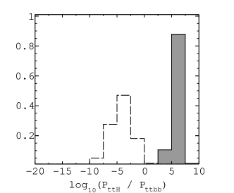
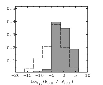
Figure 3: The event discriminant $D$ for $t\bar{t}H$ (filled) and $t\bar{t}b\bar{b}$ (dashed line) events at parton level (left) and at hadron level (right). The distributions are normalized to unit area.

Process	CPU	CPU (MP)	GPU	$\textrm{GPU}_{x}$	$\textrm{GPU}_{x}$ / CPU
signal	312	36.2	7.5	5.9	52.0
background	405	55.1	9.1	7.1	57.3

Table 3: Processing time required to evaluate the matrix elements for a single event at hadron level, for the various configurations detailed in Table 1. Note that this includes a full 8-dimensional integration over phase space for each event. Using GPU’s reduces the processing time by at least 50$\times$.

5 Conclusions

The matrix element method can be computationally prohibitive for certain final states. The benchmark study in this paper has shown that by exploiting the parallel architectures of modern GPU’s, computation time can be reduced by a factor $\geq 50$ for the matrix element method, at about 10% utilization of the GPU. It is anticipated that careful code modifications can add significant further improvements in speed. This can be the subject of future study. However, even with the performance gains in this benchmark study, it is clear that for the MEM, the computing time required with O(10) GPU’s is equivalent to a medium-sized computing cluster with O(400) cores (along with its required support and facilities infrastructure). This provides the potential to apply the method generally to searches and measurements with complex final states in experimental particle physics.

The programs described in this work are generic in nature, such that GPU-capable MEM code can be readily derived for an arbitrary $2\to N$ process with only few modifications to accommodate transformations of variables or transfer functions. It is envisaged that future work can automate the inclusion of NLO matrix elements and transformations of variables (as in MadWeight) for the matrix element method, thereby providing an optimal methodology for classification and parameter estimation in particle physics.

6 Acknowledgements

This research was enabled in part by support provided by WestGrid (www.westgrid.ca) and Compute Canada / Calcul Canada (www.computecanada.ca). We acknowledge the support of the Natural Sciences and Engineering Research Council of Canada (NSERC) and the Vice President Research Office of Simon Fraser University.

Appendix A Program Listings

typedef int   a_int_t;
typedef float a_float_t;

#ifdef _CL_CUDA_READY_ ///////////////////////////////////////////////////////// DEVICE
#ifdef _OPENCL_
#define _POW_ pow
#define _SQRT_ sqrt
#define _EXP_ exp
#define _LOG_ log
#define _ATAN_ atan
#define _TAN_ tan
#define _ACOS_ acos
#define _COS_ cos
#define _ASIN_ asin
#define _SIN_ sin
#define _CL_CUDA_HOST_
#define _CL_CUDA_DEVICE_
#define _CL_CUDA_GLOBAL_ __global
#define _CL_CUDA_CONSTANT_ __constant
#define _CL_CUDA_KERNEL_ __kernel
#endif

#ifdef _CUDA_
#define _POW_ powf
#define _SQRT_ sqrtf
#define _EXP_ expf
#define _LOG_ logf
#define _ATAN_ atanf
#define _TAN_ tanf
#define _ACOS_ acosf
#define _COS_ cosf
#define _ASIN_ asinf
#define _SIN_ sinf
#define _CL_CUDA_HOST_ __host__
#define _CL_CUDA_DEVICE_ __device__
#define _CL_CUDA_BOTH_ __host__ __device__
#define _CL_CUDA_GLOBAL_
#define _CL_CUDA_CONSTANT_
#define _CL_CUDA_KERNEL_ __global__
#endif
#else //////////////////////////////////////////////////////////////////////////// HOST
#include <cmath>
#define _POW_ std::pow
#define _SQRT_ std::sqrt
#define _EXP_ std::exp
#define _LOG_ std::log
#define _TAN_ std::tan
#define _ATAN_ std::atan
#define _COS_ std::cos
#define _ACOS_ std::acos
#define _SIN_ std::sin
#define _ASIN_ std::asin
#define _CL_CUDA_HOST_
#define _CL_CUDA_DEVICE_
#define _CL_CUDA_GLOBAL_
#define _CL_CUDA_CONSTANT_
#define _CL_CUDA_KERNEL_
#define _CL_CUDA_IDX_ 0
#endif ////////////////////////////////////////////////////////////////////////////////

Figure 4: Listing of common header used to configure the calculations for OpenCL, CUDA and C/C++ compilation.

_CL_CUDA_HOST_ _CL_CUDA_DEVICE_ a_float_t pdf(a_int_t fl,
                                              a_float_t x,
                                              a_float_t Q,
                                              _CL_CUDA_CONSTANT_ a_float_t pdf_data[],
                                              _CL_CUDA_CONSTANT_ a_float_t pdf_bounds[])
{
  if(fl < -5 || fl > 5) return 0;
  const a_int_t IOFFSET = (fl - FLAVOR_OFFSET) * (NUM_XSAMPLES_DEF * NUM_QSAMPLES_DEF);

  a_float_t pdf_lxmin = pdf_bounds[0];
  a_float_t pdf_lxmax = pdf_bounds[1];
  a_float_t pdf_lqmin = pdf_bounds[2];
  a_float_t pdf_lqmax = pdf_bounds[3];

  x = _LOG_(x);
  Q = _LOG_(Q);

  a_float_t dx = (pdf_lxmax - pdf_lxmin) / NUM_XSAMPLES_DEF;
  unsigned ix = 0;
  if(pdf_lxmin < x) ix = static_cast<unsigned int>((x - pdf_lxmin) / dx);
  ix = ix < NUM_XSAMPLES_DEF-1 ? ix : NUM_XSAMPLES_DEF-2;

  a_float_t dq = (pdf_lqmax - pdf_lqmin) / NUM_QSAMPLES_DEF;
  unsigned iq = 0;
  if(pdf_lqmin < Q) iq = static_cast<unsigned int>((Q - pdf_lqmin) / dq);
  iq = iq < NUM_QSAMPLES_DEF-1 ? iq : NUM_QSAMPLES_DEF-2;

  a_float_t c11x = pdf_lxmin + dx*ix;
  a_float_t c11q = pdf_lqmin + dq*iq;

  a_float_t c22x = pdf_lxmin + dx*(ix+1);
  a_float_t c22q = pdf_lqmin + dq*(iq+1);

  a_float_t norm = dx*dq;

  unsigned int i0j0 = iq*NUM_XSAMPLES_DEF + ix;
  unsigned int i1j0 = (iq+1)*NUM_XSAMPLES_DEF + ix;
  unsigned int i0j1 = iq*NUM_XSAMPLES_DEF + ix + 1;
  unsigned int i1j1 = (iq+1)*NUM_XSAMPLES_DEF + ix + 1;

  return (pdf_data[i0j0+IOFFSET] / (norm) * (c22x - x)*(c22q - Q) +
Ψ  pdf_data[i0j1+IOFFSET] / (norm) * (x - c11x)*(c22q - Q) +
Ψ  pdf_data[i1j0+IOFFSET] / (norm) * (c22x - x)*(Q - c11q) +
Ψ  pdf_data[i1j1+IOFFSET] / (norm) * (x - c11x)*(Q - c11q));
}

Figure 5: Listing of PDF function adapted for OpenCL & CUDA. The function takes as input a uniform grid ($x,Q$) for each parton flavor, as provided by querying any third-party PDF set. The PDF at any point in the ($x,Q$) plane is then determined using bilinear interpolation.

#ifndef cmplx_h
#define cmplx_h

#include "matcommon.h"

struct a_cmplx_t {
  a_float_t re; a_float_t im;

  _CL_CUDA_DEVICE_ a_cmplx_t()                         { }
  _CL_CUDA_DEVICE_ a_cmplx_t(a_float_t x, a_float_t y) { re = x; im = y; }
  _CL_CUDA_DEVICE_ a_cmplx_t(a_float_t x)              { re = x; im = 0; }
  _CL_CUDA_DEVICE_ a_cmplx_t(const a_cmplx_t& c)       { re = c.re; im = c.im; }

  a_cmplx_t& operator=(const a_float_t& x)  { re = x; im = 0; }
  a_cmplx_t& operator=(const a_cmplx_t& c)  { re = c.re; im = c.im; }
};

inline _CL_CUDA_DEVICE_ a_float_t real(a_cmplx_t a) { return a.re; }

inline _CL_CUDA_DEVICE_ a_float_t imag(a_cmplx_t a) { return a.im; }

inline _CL_CUDA_DEVICE_ a_cmplx_t conj(a_cmplx_t a) { return a_cmplx_t(a.re,-a.im); }

inline _CL_CUDA_DEVICE_ a_float_t fabsc(a_cmplx_t a) { return _SQRT_((a.re*a.re)+(a.im*a.im)); }

inline _CL_CUDA_DEVICE_ a_float_t fabsc_sqr(a_cmplx_t a) { return (a.re*a.re)+(a.im*a.im); }

inline _CL_CUDA_DEVICE_ a_cmplx_t operator+(a_cmplx_t a, a_cmplx_t b) { return a_cmplx_t(a.re + b.re, a.im + b.im); }

inline _CL_CUDA_DEVICE_ a_cmplx_t operator+(a_float_t a, a_cmplx_t b) { return a_cmplx_t(a + b.re, b.im); }

inline _CL_CUDA_DEVICE_ a_cmplx_t operator+(a_cmplx_t a) { return a_cmplx_t(+a.re, +a.im); }

inline _CL_CUDA_DEVICE_ a_cmplx_t operator-(a_cmplx_t a, a_cmplx_t b) { return a_cmplx_t(a.re - b.re, a.im - b.im); }

inline _CL_CUDA_DEVICE_ a_cmplx_t operator-(a_float_t a, a_cmplx_t b) { return a_cmplx_t(a - b.re, -b.im); }

inline _CL_CUDA_DEVICE_ a_cmplx_t operator-(a_cmplx_t a) { return a_cmplx_t(-a.re, -a.im); }

inline _CL_CUDA_DEVICE_ a_cmplx_t operator*(a_cmplx_t a, a_cmplx_t b) {
  return a_cmplx_t((a.re * b.re) - (a.im * b.im),
ΨΨ   (a.re * b.im) + (a.im * b.re));
}

inline _CL_CUDA_DEVICE_ a_cmplx_t operator*(a_cmplx_t a, a_float_t s) { return a_cmplx_t(a.re * s, a.im * s); }

inline _CL_CUDA_DEVICE_ a_cmplx_t operator*(a_float_t s, a_cmplx_t a) { return a_cmplx_t(a.re * s, a.im * s); }

inline _CL_CUDA_DEVICE_ a_cmplx_t operator/(a_cmplx_t a, a_cmplx_t b) {
  a_float_t t=(1./(b.re*b.re+b.im*b.im));
  return a_cmplx_t( ( (a.re * b.re) + (a.im * b.im))*t,
ΨΨ    (-(a.re * b.im) + (a.im * b.re))*t );
}

inline _CL_CUDA_DEVICE_ a_cmplx_t operator/(a_cmplx_t a, a_float_t s) { return a * (1. / s); }

inline _CL_CUDA_DEVICE_ a_cmplx_t operator/(a_float_t s, a_cmplx_t a) {
  a_float_t inv = s*(1./(a.re*a.re+a.im*a.im));
  return a_cmplx_t(inv*a.re,-inv*a.im);
}

#endif // cmplx_h

Figure 6: Listing of complex number type written for OpenCL, for which there is no native equivalent.

References

- [1] K. Kondo, Dynamical Likelihood Method for Reconstruction of Events with Missing Momentum. I. Method and Toy Models, J. Phys. Soc. Jap. 57 (12) (1988) 4126–4140. doi:10.1143/JPSJ.57.4126.
- [2] V.M. Abazov, et al, Helicity of the W boson in lepton + jets events, Phys. Lett. B 617 (2005) 1–10. doi:http://dx.doi.org/10.1016/j.physletb.2005.04.069.
- [3] Abulencia, A. et al, Precision measurement of the top-quark mass from dilepton events at cdf ii, Phys. Rev. D 75 (2007) 031105. doi:10.1103/PhysRevD.75.031105.
- [4] V. Abazov, et al., A precision measurement of the mass of the top quark, Nature 429 (2004) 638–642. arXiv:hep-ex/0406031, doi:10.1038/nature02589.
- [5] Aaltonen, T., et al, Observation of single top quark production and measurement of with CDF, Phys. Rev. D 82 (2010) 112005. doi:10.1103/PhysRevD.82.112005.
- [6] Aaltonen, T., et al, Search for a Standard Model Higgs Boson in in Collisions at TeV, Phys. Rev. Lett. 103 (2009) 101802. doi:10.1103/PhysRevLett.103.101802.
- [7] S. Chatrchyan, et al., Observation of a new boson at a mass of 125 GeV with the CMS experiment at the LHC, Phys.Lett. B716 (2012) 30–61. arXiv:1207.7235, doi:10.1016/j.physletb.2012.08.021.
- [8] Search for the Standard Model Higgs boson in the decay mode using Multivariate Techniques with 4.7 fb-1 of ATLAS data at TeV, Tech. Rep. ATLAS-CONF-2012-060, CERN, Geneva (June 2012).
- [9] F. Fiedler, A. Grohsjean, P. Haefner, and P. Schieferdecker, The Matrix Element Method and its Application to Measurements of the Top Quark Mass, NIM A 624 (1) (2010) 203–218. doi:10.1016/j.nima.2010.09.024.
- [10] A. Grohsjean, Measurement of the Top Quark Mass in the Dilepton Final State Using the Matrix Element Method, 2010. doi:10.1007/978-3-642-14070-9\_5.
- [11] P. Artoisenet, V. Lemaitre, F. Maltoni, and O. Mattelaer, Automation of the matrix element reweighting method, JHEP 12 (68). doi:10.1007/JHEP12(2010)068.
- [12] K. Hagiwara, J. Kanzaki, Q. Li, N. Okamura, T. Stelzer, Fast computation of MadGraph amplitudes on graphics processing unit (GPU), European Physical Journal C 73 (2013) 2608. arXiv:1305.0708, doi:10.1140/epjc/s10052-013-2608-2.
- [13] F. Englert, R. Brout, Broken symmetry and the mass of gauge vector mesons, Phys. Rev. Lett. 13 (1964) 321–323. doi:10.1103/PhysRevLett.13.321.
- [14] Higgs, Peter W., Broken Symmetries and the Masses of Gauge Bosons, Phys. Rev. Lett. 13 (1964) 508–509. doi:10.1103/PhysRevLett.13.508.
- [15] G. S. Guralnik, C. R. Hagen, T. W. B. Kibble, Global conservation laws and massless particles, Phys. Rev. Lett. 13 (1964) 585–587. doi:10.1103/PhysRevLett.13.585.
- [16] S. Dittmaier, S. Dittmaier, C. Mariotti, G. Passarino, R. Tanaka, et al., Handbook of LHC Higgs Cross Sections: 2. Differential DistributionsarXiv:1201.3084, doi:10.5170/CERN-2012-002.
- [17] C. Degrande, J. Gerard, C. Grojean, F. Maltoni, G. Servant, Probing Top-Higgs Non-Standard Interactions at the LHC, JHEP 1207 (2012) 036. arXiv:1205.1065, doi:10.1007/JHEP07(2012)036,10.1007/JHEP03(2013)032.
- [18] G. Peter Lepage, A new algorithm for adaptive multidimensional integration, Journal of Computational Physics 27 (2) (1978) 192 – 203. doi:http://dx.doi.org/10.1016/0021-9991(78)90004-9.
- [19] G. Peter Lepage, VEGAS: An Adaptive Multi-dimensional Integration Program, Tech. Rep. CLNS 80-447, Cornell (March 1980).
- [20] J. Nickolls, I. Buck, M. Garland, K. Skadron, Scalable parallel programming with cuda, Queue 6 (2) (2008) 40–53. doi:10.1145/1365490.1365500.
- [21] J. E. Stone, D. Gohara, G. Shi, Opencl: A parallel programming standard for heterogeneous computing systems, IEEE Des. Test 12 (3) (2010) 66–73. doi:10.1109/MCSE.2010.69.
-
[22]
Ofer Rosenberg, Benedict R. Gaster, Bixia Zheng, Irina Lipov,
OpenCL
Static C++ Kernel Language Extension, 04 Edition (2012).
URL {http://amd-dev.wpengine.netdna-cdn.com/wordpress/media/2012/10/CPP_kernel_language.pdf} - [23] L. Sonnenschein, Algebraic approach to solve dilepton equations, Phys. Rev. D 72 (2005) 095020. doi:10.1103/PhysRevD.72.095020.
- [24] Alwall, Johan and Herquet, Michel and Maltoni, Fabio and Mattelaer, Olivier and Stelzer, Tim, MadGraph 5 : Going Beyond, JHEP 1106 (2011) 128. arXiv:1106.0522, doi:10.1007/JHEP06(2011)128.
- [25] H. Murayama, I. Watanabe, K. Hagiwara, HELAS: HELicity amplitude subroutines for Feynman diagram evaluations.
- [26] P. de Aquino, W. Link, F. Maltoni, O. Mattelaer, T. Stelzer, ALOHA: Automatic Libraries Of Helicity Amplitudes for Feynman Diagram Computations, Comput.Phys.Commun. 183 (2012) 2254–2263. arXiv:1108.2041, doi:10.1016/j.cpc.2012.05.004.
- [27] M. Whalley, D. Bourilkov, R. Group, The Les Houches accord PDFs (LHAPDF) and LHAGLUEarXiv:hep-ph/0508110.
- [28] Lai, Hung-Liang and Guzzi, Marco and Huston, Joey and Li, Zhao and Nadolsky, Pavel M. and others, New parton distributions for collider physics, Phys.Rev. D82 (2010) 074024. arXiv:1007.2241, doi:10.1103/PhysRevD.82.074024.
- [29] T. Sjostrand, S. Mrenna, P. Z. Skands, PYTHIA 6.4 Physics and Manual, JHEP 0605 (2006) 026. arXiv:hep-ph/0603175, doi:10.1088/1126-6708/2006/05/026.
- [30] P. Z. Skands, Tuning Monte Carlo Generators: The Perugia Tunes, Phys.Rev. D82 (2010) 074018. arXiv:1005.3457, doi:10.1103/PhysRevD.82.074018.
- [31] M. Cacciari, G. P. Salam, G. Soyez, FastJet User Manual, Eur.Phys.J. C72 (2012) 1896. arXiv:1111.6097, doi:10.1140/epjc/s10052-012-1896-2.
- [32] A. Klöckner, N. Pinto, Y. Lee, B. Catanzaro, P. Ivanov, A. Fasih, PyCUDA and PyOpenCL: A Scripting-Based Approach to GPU Run-Time Code Generation, Parallel Computing 38 (3) (2012) 157–174. doi:10.1016/j.parco.2011.09.001.
-
[33]
G. Peter Lepage,
vegas
Documentation, 2.1.4 Edition (2014).
URL {http://github.com/gplepage/vegas/blob/master/doc/vegas.pdf}