Dynamic Feature Scaling for
Online Learning of Binary Classifiers

Abstract

Scaling feature values is an important step in numerous machine learning tasks. Different features can have different value ranges and some form of a feature scaling is often required in order to learn an accurate classifier. However, feature scaling is conducted as a preprocessing task prior to learning. This is problematic in an online setting because of two reasons. First, it might not be possible to accurately determine the value range of a feature at the initial stages of learning when we have observed only a few number of training instances. Second, the distribution of data can change over the time, which render obsolete any feature scaling that we perform in a pre-processing step. We propose a simple but an effective method to dynamically scale features at train time, thereby quickly adapting to any changes in the data stream. We compare the proposed dynamic feature scaling method against more complex methods for estimating scaling parameters using several benchmark datasets for binary classification. Our proposed feature scaling method consistently outperforms more complex methods on all of the benchmark datasets and improves classification accuracy of a state-of-the-art online binary classifier algorithm.

1 Introduction

Machine learning algorithms require train and test instances to be represented using a set of features. For example, in supervised document classification [6], a document is often represented as a vector of its words and the value of a feature is set to the number of times the word corresponding to the feature occurs in that document. However, different features occupy different value ranges, and often one must scale the feature values before any supervised classifier is trained. In our example of document classification, there are both highly frequent words (e.g. stop words) as well as extremely rare words. Often, the relative difference of a value of a feature is more informative than its absolute value. Therefore, feature scaling has shown to improve performance in classification algorithms.

Typically, feature values are scaled to a standard range in a preprocessing step before using the scaled features in the subsequent learning task. However, this preprocessing approach to feature value scaling is problematic because of several reasons. First, often feature scaling is done in an unsupervised manner without consulting the labels assigned to the training instances. Although this is the only option in unsupervised learning tasks such as document clustering, for supervised learning tasks such as document classification, where we do have access to the label information, we can use the label information also for feature scaling. Second, it is not possible to perform feature scaling as a preprocessing step in one-pass online learning setting. In one-pass online learning we are allowed to traverse through the set of training instances only once. Learning from extremely large datasets such as twitter streams or Web scale learning calls for algorithms that require only a single pass over the set of training instances. In such scenarios it is not possible to scale the feature values beforehand by using statistics from the entire training set. Third, even if we pre-compute scaling parameters for a feature, those values might become obsolete in an online learning setting in which the statistical properties of the training instances vary over the time. For example, a twitter text stream regarding a particular keyword might change overtime and the scaling factors computed using old data might not be appropriate for the new data.

We study the problem of dynamically scaling feature values at run time for online learning. The term dynamic feature scaling is used in this paper to refer to the practice of scaling feature values at run time as opposed to performing feature scaling as a pre-processing step that happens prior to learning. We focus on binary classifiers as a specific example. However, we note that the proposed method can be easily extended to multi-class classifiers. We propose two main approaches for dynamic feature scaling in this paper: (a) Unsupervised Dynamic Feature Scaling (Section 3), in which we do not consider the label information assigned to the training instances for feature scaling, and (b) Supervised Dynamic Feature Scaling (Section 4), in which we consider the label information assigned to the training instances for feature scaling.

All algorithms we propose in this paper can be trained under the one-pass online learning setting, where only a single training instance is provided at a time and only the scale parameters and feature weights are stored in the memory. This enables the proposed method to (a) efficiently adapt to the varying statistics in the data stream, (b) compute the optimal feature scales such that the likelihood of the training data under the trained model is maximized, and (c) train from large datasets where batch learning is impossible because of memory requirements. We evaluate the proposed methods in combination with different online learning algorithms using three benchmark datasets for binary classification. Our experimental results show that, interestingly, the much simpler unsupervised dynamic feature scaling method consistently improves all of the online binary classification algorithms we compare, including the state-of-the-art classifier of [6].

2 Related Work

Online learning has received much attention lately because of the necessity to learn from large training datasets such as query logs in a web search engine [22], web-scale document classification or clustering [19], and sentiment analysis on social media [15, 11]. Online learning toolkits that can efficiently learn from large datasets are made available such as Vowpal Wabbit and OLL (Online Learning Library). Online learning approaches are attractive than their batch learning counterparts when the training data involved is massive due to two main reasons. First, the entire dataset might not fit into the main memory of a single computer to perform a batch optimization. Although there has been some recent progress in distributed learning algorithms [14, 13, 17] that can distribute the batch optimization process across a series of machines, setting up and debugging such a distributed learning environment remains a complex process. On the other hand, online learning algorithms consider only a small batch (often referred to as a mini batch in the literature) or in the extreme case a single training instance. Therefore, the need for large memory spaces can be avoided with online learning. Second, a batch learning algorithm requires at least one iteration over the entire dataset to produce a classifier. This can be time consuming for large training datasets. On the other hand, online learning algorithms can produce a relatively accurate classifier even after observing a handful of training instances.

Online learning is a vast and active research field and numerous algorithms have been proposed in prior work to learn classifiers [7, 8, 20, 21, 12, 18]. A detailed discussion of online classification algorithms is beyond the scope of this paper. Some notable algorithms are the passive-aggressive (PA) algorithms [6], confidence-weighted linear classifiers [10] and their multi-class variants [7, 8]. In passive-aggressive learning, the weight vector for the binary classifier is updated only when a misclassification occurs. If the current training instance can be correctly classified using the current weight vector, then the weight vector is not updated. In this regard, the algorithm is considered passive. On the other hand, if a misclassification occurs, then the weight vector is aggresively updated such that it can correctly classify the current training instance with a fixed margin. Passive-aggressive algorithm has consistently outperformed numerous other online learning algorithms across a wide-range of tasks. Therefore, it is considered as a state-of-the-art online binary classification algorithm. As we demonstrate later, the unsupervised dynamic feature scaling method proposed in this paper further improves the accuracy of the passive-aggressive algorithm. Moreover, active-learning [9] and transfer learning [24] approaches have also been proposed for online classifier learning.

One-Pass Online Learning (OPOL) (also known as stream learning) [11] is a special case of online learning in which only a single-pass is allowed over the set of train instances by the learning algorithm. Typically, an online learning algorithm requires multiple passes over a training dataset to reach a convergent point. This setting can be considered as an extreme case where the train batch size is limited to only one instance. The OPOL setting is more restrictive than the classical online learning setting where a learning algorithm is allowed to traverse multiple times over the training dataset. However, OPOL becomes the only possible alternative in the following scenarios.

1. The number of instances in the training dataset is so large that it is impossible to traverse multiple times over the dataset.

2. The dataset is in fact a stream where we encounter new instances continuously. For example, consider the situation where we want to train a sentiment classifier from tweets.

3. The data stream changes over time. In this case, even if we can store old data instances they might not be much of a help to predict the latest trends in the data stream.

It must be noted that OPOL is not the only solution for the first scenario where we have a large training dataset. One alternative approach is to select a subset of examples from the dataset at each iteration and only use that subset for training in that iteration. One promising criterion for selecting examples for training is curriculum learning [1]. In curriculum learning, a learner is presented with easy examples first and gradually with the more difficult examples. However, determining the criteria for selecting easy examples is a difficult problem itself, and the criterion for selecting easy examples might be different from one task to another. Moreover, it is not clear whether we can select easy examples from the training dataset in a sequential manner as required by online learning without consulting the unseen training examples.

The requirement for OPOL ever increases with the large training datasets and data streams we encounter on the Web such as social feeds. Most online learning algorithms require several passes over the training dataset to achieve convergence. For example, Passive-Aggressive algorithms [6] require at least $5$ iterations over the training dataset to converge, whereas, for Confidence-Weighted algorithms [10] the number of iterations has shown to be less (ca. $2$). Our focus in this paper is not to develop online learning algorithms that can classify instances with high accuracy by traversing only once over the dataset, but to study the effect of feature scaling in the OPOL setting. To this end, we study both an unsupervised dynamic feature scaling method (Section 3) and several variants of a supervised dynamic feature scaling methods (Section 4).

3 Unsupervised Dynamic Feature Scaling

In unsupervised dynamic feature scaling, given a feature $x_{j}$, we compute the mean, $\mu(x_{j})$ and the standard deviation $\delta(x_{j})$ of the feature and perform an affine transformation as follows,

$$x_{j}^{\prime}=\frac{x_{j}-\mu_{j}}{\delta_{j}}.$$ (1)

This scaling operation corresponds to a linear shift of the feature values by the mean value of the feature, followed up by a scaling by its standard deviation. From a geometric point of view, this transformation will shift the origin to the mean value and then scale axis corresponding to the $j$-th feature to unit standard deviation. It is used popularly in batch learning setting, in which one can compute the mean and the standard deviation using all the training instances in the training dataset. However, this is not possible in OPOL, in which we encounter only one instance at a time. However, even in the OPOL setting, we can compute the mean and the standard deviation on the fly and constantly update our estimates of those values as new training instances (feature vectors) are observed. The update equations for the mean $m^{k}_{j}$ and the standard deviation $\sqrt{s^{k}_{j}/(k-1)}$ for the $j$-th feature are as follows [16, 4],

$$m^{k}_{j} = m^{k-1}_{j}+\frac{x^{k}_{j}-m^{k-1}_{j}}{k},$$ (2)

$$s^{k} = s^{k-1}+(x^{k}_{j}-m^{k-1}_{j})(x^{k}_{j}-m^{k}_{j}).$$ (3)

We use these estimates for the mean and the standard deviation to scale features in Equation 1. The mean and standard deviation are updated throughout the training process.

4 Supervised Dynamic Feature Scaling

We define the task of supervised dynamic feature scaling task for binary classification in the OPOL setting as follows. Given a stream of labeled training instances $(\boldsymbol{x}_{n},t_{n})$, in which the class label $t_{n}$ of the $n$-th training instance $x_{n}$, denoted by a feature vector $\boldsymbol{x}_{n}$, is assumed to be either $+1$ (positive class) or $-1$ (negative class). Furthermore, let us assume that the feature space is $M$ dimensional and the value of the $i$-th feature of the $n$-th instance in the training data stream is denoted by $x_{i}^{n}$. In this paper, we consider only real-valued features (i.e. $x_{i}^{n}\in\mathbb{R}$) because feature scaling is particularly important for real-valued features.

We define the feature scaling function $\sigma_{i}(x_{i}^{n})$ for the $i$-th feature as a function that maps $\mathbb{R}$ to the range $[0,1]$ as follows:

$$\sigma_{i}(x_{i}^{n})=\frac{1}{1+\exp(-\alpha_{i}x_{i}^{n}+\beta_{i})}.$$ (4)

Here, $\alpha_{i}$ and $\beta_{i}$ are the scaling parameters for the $i$-th dimension of the feature space. Several important properties of the feature scaling function defined by Equation 4 are noted. First, the feature transformation function maps all feature values to the range $[0,1]$ irrespective of the original range in which each feature value $x_{i}$ was. For example, one feature might originally be limited to the range $[0,0.001]$, whereas another feature might have values in the full range of $[0,10000]$. By scaling each feature into a common range we can concentrate on the relative values of those features without being biased by their absolute values. Second, the scaling parameters $\alpha_{i}$ and $\beta_{i}$ are defined per-feature basis. This enables us to scale different features using scale parameters appropriate for their value ranges. Third, the linear transformation $\alpha_{i}x_{i}^{n}-\beta_{i}$ within the exponential term of the feature scaling function resembles the typical affine transformations performed in unsupervised feature scaling. For example, assuming the mean and the standard deviation of the $i$-th feature to be respectively $\mu_{i}$ and $\delta_{i}$, in supervised classification, features are frequently scaled to $(x_{i}-\mu_{i})/\delta_{i}$ prior to training and testing. The linear transformation within the exponential term in Equation 4 can be seen as a special case of this approach with values $\alpha_{i}=1/\delta_{i}$ and $\beta_{i}=\mu_{i}/\delta_{i}$.

Then, the posterior probability, $P(t=1|\boldsymbol{x}^{n},b,\boldsymbol{\alpha},\boldsymbol{\beta})$ of $\boldsymbol{x}^{n}$ belonging to the positive class is given as follows according to the logistic regression model [3]:

$$P(t_{n}=1|\boldsymbol{x}^{n},b,\boldsymbol{\alpha},\boldsymbol{\beta})=\frac{1}{1+\exp\left(-\sum_{i=1}^{M}w_{i}\sigma_{i}(x_{i}^{n})-b\right)},$$ (5)

$$P(t_{n}=1|\boldsymbol{x}^{n},b,\boldsymbol{\alpha},\boldsymbol{\beta})=\frac{1}{1+\exp\left(-\frac{w_{i}}{1+\exp(-\alpha_{i}x_{i}^{n}+\beta_{i})}-b\right)}.$$

Here, $w_{i}$ is the weight associated with the $i$-th feature and $b\in\mathbb{R}$ is the bias term. We arrange the weights $w_{i}$, scaling parameters $\alpha_{i}$ and $\beta_{i}$ respectively using $\mathbb{R}^{M}$ vectors $\boldsymbol{w}$, $\boldsymbol{\alpha}$, and $\boldsymbol{\beta}$.

The cross-entropy loss function per instance including the L2 regularization terms for the weight vector $\boldsymbol{w}$ and scale vector $\boldsymbol{\beta}$ can be written as follows:

$$L(\boldsymbol{w},b,\boldsymbol{\alpha},\boldsymbol{\beta})=-t_{n}\log y_{n}-(1-t_{n})\log(1-y_{n})$$ (6)

Here, we used $y_{n}=P(t=1|\boldsymbol{x}^{n},b,\boldsymbol{\alpha},\boldsymbol{\beta})$ to minimize the cluttering of symbols in Equation 6. To avoid overfitting to training instances and to minimize the distortion of the training instances, we impose L2 regularization on $\boldsymbol{w}$, $\boldsymbol{\alpha}$, and $\boldsymbol{\beta}$. Therefore, the final objective function that must be minimized with respect to $\boldsymbol{w}$, $\boldsymbol{\alpha}$, $\boldsymbol{\beta}$, and $b$ is give by,

$$E(\boldsymbol{w},b,\boldsymbol{\alpha},\boldsymbol{\beta})=L(\boldsymbol{w},b,\boldsymbol{\alpha},\boldsymbol{\beta})+\lambda\left|\left|w\right|\right|_{2}^{2}+\mu\left|\left|\alpha\right|\right|_{2}^{2}+\nu\left|\left|\beta\right|\right|_{2}^{2}$$ (7)

Here, $\lambda$, $\mu$ and $\nu$ respectively are the L2 regularization coefficients corresponding to the weight vector $\boldsymbol{w}$ and the scale vectors $\boldsymbol{\alpha}$, $\boldsymbol{\beta}$. Because we consider the minimization of Equation 7 per instance basis, in our experiments, we divide the regularization parameters $\lambda$, $\mu$, and $\nu$ by the total number of training instances $N$ in the dataset such that we can compare the values those parameters across datasets of different sizes.

By setting the partial derivatives $\frac{\partial E}{\partial w_{j}}$, $\frac{\partial E}{\partial b}$, $\frac{\partial E}{\partial\alpha_{j}}$, and $\frac{\partial E}{\partial\beta_{j}}$ to zero and applying Stochastic Gradient Descent (SGD) update rule the following updates can be derived,

$$w_{j}^{k+1}=w_{j}^{k}(1-2\lambda\eta_{k})+\eta_{k}(t_{n}-y_{n})\sigma_{j}(x^{n}_{j}),$$ (8)

$$b^{k+1}=b^{k}+\eta_{k}(t_{n}-y_{n}),$$ (9)

$$\alpha_{j}^{k+1} =\alpha_{j}^{k}(1-2\mu\eta_{k})+\eta_{k}x^{n}_{j}w_{j}\sigma_{j}(x^{n}_{j})(1-\sigma_{j}(x^{n}_{j}))(t_{n}-y_{n}),$$ (10)

$$\beta_{j}^{k+1} =\beta_{j}^{k}(1-2\nu\eta_{k})-\eta_{k}(t_{n}-y_{n})w_{j}\sigma_{j}(x^{n}_{j})(1-\sigma_{j}(x^{n}_{j})).$$ (11)

In Equations 8-11, $k$ denotes the $k$-th update and $\eta_{k}$ is the learning rate for the $k$-th update. We experimented with both linear and exponential decaying and found linear decaying to perform better for the proposed method. The linear decaying function for $\eta_{k}$ is defined as follows,

$$\eta_{k}=\frac{\eta_{0}}{1+\frac{k}{T\times N}}.$$ (12)

Here, $T$ is the total number of iterations for which the training dataset containing $N$ instances will be traversed. Because we are considering OPOL, we set $T=1$. The initial learning rate $\eta_{0}$ is set to $0.1$ throughout the experiments described in the paper. This value of $0.1$ was found to be producing the best results in our preliminary experiments using development data, which we selected randomly from the benchmark datasets described later in Section 5.

Several observations are in order. First, note that the scaling factors $\alpha_{j}$ and $\beta_{j}$ distort the original value of the feature $x_{i}$. If this distortion is too much, then we might loose the information conveyed by the feature $x_{i}$. To minimize the distortion of $\boldsymbol{x}$ because of scaling, we have imposed regularization on both $\boldsymbol{\alpha}$ and $\boldsymbol{\beta}$. This treatment is similar to the slack variables often used in non-separable classification tasks and imposing a penalty on the total slackness. Of course, the regularization on $\boldsymbol{\alpha}$ and $\boldsymbol{\beta}$ can be removed simply by setting the corresponding regularization coefficients $\mu$ and $\nu$ to zero. Therefore, the introduction of regularization on $\boldsymbol{\alpha}$ and $\boldsymbol{\beta}$ does not harm the generality of the proposed method. The total number of parameters to train in this model is $M+M+M+1=3M+1$, corresponding to $\boldsymbol{w}$, $\boldsymbol{\alpha}$, $\boldsymbol{\beta}$, and $b$. Note that we must not regularize the bias term $b$ and let it to adjust arbitrarily. This can be seen as a dynamic scaling for the score (i.e. inner-product between $\boldsymbol{w}$ and $\boldsymbol{x}$), although this type of scaling is not feature specific. The sigmoid-based feature scaling function given by Equation 4 is by no means the only function that satisfies the requirement for a scaling function (i.e. maps all feature values to the same range such as $[0,1]$). However, the sigmoid function has been widely used in various fields of machine learning such as neural networks [23], and has desirable properties such as differentiability and continuity.

Next, we introduce several important variants of Equation 4 and present the update equations for each of those variants. In Section 6, we empirically study the effect of the different variants discussed in the paper. For the ease of reference, we name the original formulation given by Equation 4 as FS (Supervised Feature Scaling) method. The objective function given by Equation 7 is convex with respect to $\boldsymbol{w}$. This can be easily verified by computing the second derivative of the objective function with respect to $w_{i}$, which becomes

$$\frac{\partial^{2}E}{\partial w_{i}^{2}}={\sigma(x_{i})}^{2}y_{n}(1-y_{n})+2\lambda.$$ (13)

Because $0<\sigma(x_{i})<1$, $0<y_{n}<1$, and $0<\lambda$ hold, the second derivative $\frac{\partial^{2}E}{\partial w_{i}^{2}}>0$, which proves that the objective function is convex with respect to $w_{i}$. Likewise, the objective function can be shown to be convex with respect to the bias term $b$. It is interesting to note that the convexity holds irrespective of the form of the scaling function $\sigma$ for both $\boldsymbol{w}$ and $b$ as long as $\sigma(x_{i})\neq 0$ is satisfied. If $\sigma(x_{i})=0$ for some value of $x_{i}$, then the convexity of $E$ also depends upon $\lambda$ not being equal to zero. Although, in the case of sigmoid feature scaling functions $\sigma(x_{i})\to 0$ when $x_{i}\to-\infty$ this is irrelevant because feature values are finite in practice. Unfortunately, the objective function is non-convex with respect to $\boldsymbol{\alpha}$ and $\boldsymbol{\beta}$. Although SGD updates are empirically shown to work well even when the objective function is non-convex, there is no guarantee that the update Equations 8 - 11 will find the global minimum of the objective function.

4.1 FS-1

In this variant we fix the scaling factor $\boldsymbol{\alpha}=\boldsymbol{1}$, thereby reducing the number of parameters to be tuned. However, this model cannot adjust for the different value ranges of features and can only learn the shiftings required. We name this variant as FS-1 and is given by,

$$\sigma_{i}(x_{i}^{n})=\frac{1}{1+\exp(-x_{i}^{n}+\beta_{i})}.$$ (14)

The update equations for $w_{j}$, $b$, and $\beta_{j}$ are as follows,

$$w_{j}^{k+1}=w_{j}^{k}(1-2\lambda\eta_{k})+\eta_{k}(t_{n}-y_{n})\sigma_{j}(x^{n}_{j}),$$ (15)

$$b^{k+1}=b^{k}+\eta_{k}(t_{n}-y_{n}),$$ (16)

$$\beta_{j}^{k+1} =\beta_{j}^{k}(1-2\nu\eta_{k})-\eta_{k}(t_{n}-y_{n})w_{j}\sigma_{j}(x^{n}_{j})(1-\sigma_{j}(x^{n}_{j})).$$ (17)

Note that although the update Equations 15, 16, and 17 appear to be similar in their form to Equations 8, 9, and 11, the transformation functions in the two sets of equations are different. As discussed earlier under FS, FS-1 is also convex with respect to $\boldsymbol{w}$ and $b$, but non-convex with respect to $\boldsymbol{\beta}$.

4.2 FS-2

We design a convex form of the objective function with respect to all parameters by replacing the sigmoid feature scaling function with a linear combination as follows,

$$\sigma_{i}(x_{i})=\alpha_{i}x_{i}+\beta_{i}.$$ (18)

The class conditional probability is computed using the logistic sigmoid model as,

$$P(t_{n}=1|\boldsymbol{w},b,\boldsymbol{\alpha},\boldsymbol{\beta})=\frac{1}{1+\exp(-\sum_{j=1}^{M}w_{j}(\alpha_{j}x^{n}_{j}+\beta_{j})-b)}.$$ (19)

Then the update equations for $\boldsymbol{w}$, $b$, $\boldsymbol{\alpha}$, and $\boldsymbol{\beta}$ are given as follows,

$$w^{k+1}_{j}=w^{k}_{j}(1-2\lambda\eta_{k})-\eta_{k}(y_{n}-t_{n})(\alpha_{j}x^{n}_{j}+\beta_{j}),$$ (20)

$$b^{k+1}=b^{k}-\eta_{k}(y_{n}-t_{n}),$$ (21)

$$\alpha^{k+1}_{j}=\alpha^{k}_{j}(1-2\mu\eta_{k})-\eta_{k}(y_{n}-t_{n})w_{j}x^{n}_{j},$$ (22)

$$\beta^{k+1}_{j}=\beta^{k}_{j}(1-2\nu\eta_{k})-\eta_{k}(y_{n}-t_{n})w_{j}.$$ (23)

Here, we used $y_{n}=P(t_{n}=1|\boldsymbol{w},b,\boldsymbol{\alpha},\boldsymbol{\beta})$ to simplify the equations.

Moreover, the second-order partial derivatives of the objective function $E$, with respect to $\boldsymbol{w}$, $b$, $\boldsymbol{\alpha}$, and $\boldsymbol{\beta}$ can be computed as follows,

$$\frac{\partial^{2}E}{\partial w_{j}^{2}} = y_{n}(1-y_{n}){(\alpha_{j}x^{n}_{j}+\beta_{j})}^{2}+2\lambda,$$

$$\frac{\partial^{2}E}{\partial\alpha_{j}^{2}} = y_{n}(1-y_{n})w_{j}^{2}x^{n2}_{j}+2\mu,$$

$$\frac{\partial^{2}E}{\partial\beta_{j}^{2}} = y_{n}(1-y_{n})w_{j}^{2}x^{n2}_{j}+2\mu,$$

$$\frac{\partial^{2}E}{\partial w_{j}^{2}} = y_{n}(1-y_{n}).$$

From, $0<y_{n}<1$, $\lambda>0$, $\mu>0$, and $\nu>0$ it follows that all of the above-mentioned second-order derivatives are positive, which proofs the convexity of the objective function. We name this convex formulation of the feature scaling method as the FS-2 method.

4.3 FS-3

Although FS-2 is convex, there is an issue regarding the determinability among $\boldsymbol{w}$, $\boldsymbol{\alpha}$, and $\boldsymbol{\beta}$ because the product between $\boldsymbol{w}$ and $\boldsymbol{\alpha}$, and the product between $\boldsymbol{w}$ and $\boldsymbol{\beta}$ appear inside the exponential term in Equation 19. This implies that the probability $P(t_{n}=1|\boldsymbol{w},b,\boldsymbol{\alpha},\boldsymbol{\beta})$ will be invariant under a constant scaling of $\boldsymbol{w}$, $\boldsymbol{\alpha}$, and $\boldsymbol{\beta}$. We can absorb the $w_{j}$ terms from the objective function into the corresponding $\alpha_{j}$ and $\beta_{j}$ terms thereby effectively both reducing the number of parameters to be trained as well as eliminating the issue regarding the determinability. We name this variant of the feature scaling method as the FS-3 method.

The class conditional probability for FS-3 is give by,

$$P(t_{n}=1|b,\boldsymbol{\alpha},\boldsymbol{\beta})=\frac{1}{1+\exp(-\sum_{j=1}^{M}(\alpha_{j}x^{n}_{j}+\beta_{j})-b)}.$$ (24)

This can be seen as a special case of FS-2 where we set $\boldsymbol{w}=\boldsymbol{1}$ and $\lambda=0$.

The update equations for FS-3 can be derived as follows,

$$b^{k+1}=b^{k}-\eta_{k}(y_{n}-t_{n}),$$ (25)

$$\alpha^{k+1}_{j}=\alpha^{k}_{j}(1-2\mu\eta_{k})-\eta_{k}(y_{n}-t_{n})x^{n}_{j},$$ (26)

$$\beta^{k+1}_{j}=\beta^{k}_{j}(1-2\nu\eta_{k})-\eta_{k}(y_{n}-t_{n}).$$ (27)

Here, we used $y_{n}=P(t_{n}=1|b,\boldsymbol{\alpha},\boldsymbol{\beta})$ to simplify the equations. Because FS-2 is convex and FS-3 is a special case of FS-2, it follows that FS-3 is also convex.

5 Datasets

To evaluate the performance of the numerous feature scaling methods introduced in Section 4, we train and test those methods under the one-pass online learning setting. We use three datasets in our experiments: heart dataset, liver dataset, and the diabetes dataset. All three datasets are popularly used as benchmark datasets to evaluate binary classification algorithms. Moreover, all three datasets contain real-valued and unscaled features values, which are appropriate for the current evaluation purpose. All three datasets can be downloaded from the UCI Machine Learning Repository. Details of the three datasets are summarized in Table 1.

Table 1: Statistics regarding the three datasets used in the experiments.

Dataset	Attributes	Train instances	Test instances
heart	$13$	$216$	$54$
liver	$6$	$276$	$69$
diabetes	$8$	$611$	$157$

6 Experiments and Results

To compare the performance of the different dynamic feature scaling methods we proposed in the paper, we use those methods to scale features in the following online learning algorithms.

SGD (Stochastic Gradient Descent):

This method implements logistic regression using stochastic gradient descent. It does not use any feature scaling and uses the original feature values as they are for training a binary classifier. This method demonstrates the lower baseline performance for this task.

SDG+avg (Stochastic Gradient Descent with Model Averaging):

This method is the same as SGD described above, except that it uses the average weight vector during training and testing. Specifically, it computes the average of the weight vector $\boldsymbol{w}$ over the updates and uses this average vector for prediction. By considering the average weight vector instead of the final weight vector we can avoid any bias toward the last few training instances encountered by the online learner. Moreover, it has been shown both theoretically and empirically that consideration of the average weight vector results in faster convergence in online learning [5].

GN (Unsupervised Dynamic Scaling):

This is the unsupervised dynamitc feature scaling method described in Section 3. It trains a binary logistic regression model by scaling the features using the unsupervised approach.

GN+avg (Unsupervised Dynamic Scaling with Model Averaging):

This is the unsupervised feature scaling method described in Section 3 using the average weight vector for predicting instead of the final weight vector. It trains a binary logistic regression model by scaling the features using the unsupervised approach.

FS (Supervised Dynamic Feature Scaling):

This is the supervised dynamic feature scaling method described in Section 4.

FS+avg (Supervised Dynamic Feature Scaling with Model Averaging):

This is the FS method, where we use the average values for all parameters: $\boldsymbol{w}$, $b$, $\boldsymbol{\alpha}$, and $\boldsymbol{\beta}$.

FS-1 (Supervised Dynamic Feature Scaling variant FS-1):

This is the method described in Section 4.1.

FS-1+avg (Supervised Dynamic Feature Scaling variant FS-1 with Model Averaging):

This is the method described in Section 4.1 with averaged parameter vectors.

FS-2 (Supervised Dynamic Feature Scaling variant FS-2):

This is the method described in Section 4.2.

FS-2+avg (Supervised Dynamic Feature Scaling variant FS-1 with Model Averaging):

This is the method described in Section 4.2 with averaged parameter vectors.

FS-3 (Supervised Dynamic Feature Scaling variant FS-3):

This is the method described in Section 4.3.

FS-3+avg (Supervised Dynamic Feature Scaling variant FS-1 with Model Averaging):

This is the method described in Section 4.3 with averaged parameter vectors.

PA (Passive-Aggressive):

This is the Passive-Aggressive binary linear classification algorithm proposed by [6].

PA+avg (Passive-Aggressive with Model Averaging):

This is the Passive-Aggressive binary linear classification algorithm proposed by [6] using the averaged weight vector to predict during both training and testing stages.

PA-1 (Passive-Average variant 1):

This is the Passive-Aggressive PA-I version of the binary linear classification algorithm proposed by [6].

PA-1+avg (Passive-Aggressive variant 1 with Model Averaging):

This is the Passive-Aggressive PA-1 version of the binary linear classification algorithm proposed by [6] using the averaged weight vector to predict during both training and testing stages.

PA-2 (Passive-Aggressive variant 2):

This is the Passive-Aggressive PA-2 version of the binary linear classification algorithm proposed by [6].

PA-2+avg (Passive-Aggressive variant 2 with Model Averaging):

This is the Passive-Aggressive PA-2 version of the binary linear classification algorithm proposed by [6] using the averaged weight vector to predict during both training and testing stages.

Table 2: Results on the heart dataset.

Algorithm	Train Accuracy	Test Accuracy	Best Parameters
SGD	$0.537037$	$0.574074$	$\lambda=0.01$
SGD+avg	$0.481481$	$0.435185$	$\lambda=0$
GN	$\mathbf{0.87037}$	$\mathbf{0.824074}$	$\lambda=0.01$
GN+avg	$0.777778$	$0.768519$	$\lambda=0.1$
FS	$0.592593$	$0.49537$	$\lambda=0.1,\mu=1.0,\nu=0$
FS+avg	$0.481481$	$0.435185$	$\lambda=0,\mu=0\nu=0$
FS-1	$0.703704$	$0.564815$	$\mu=100.0,\nu=0.1$
FS-1+avg	$0.759259$	$0.564815$	$\mu=0.1,\nu=10.0$
FS-2	$0.740741$	$0.569444$	$\lambda=10.0,\mu=0,\nu=10.0$
FS-2+avg	$0.574074$	$0.467593$	$\lambda=0,\mu=1.0,\nu=0$
FS-3	$0.592593$	$0.476852$	$\mu=0.1,\nu=0$
FS-3+avg	$0.574074$	$0.421296$	$\mu=0.1,\nu=1.0$
PA	$0.648148$	$0.675926$	$c=0.01$
PA+avg	$0.611111$	$0.662037$	$c=0.01$
PA1	$0.648148$	$0.675926$	$c=0.01$
PA1+avg	$0.611111$	$0.662037$	$c=0.01$
PA2	$0.648148$	$0.675926$	$c=0.01$
PA2+avg	$0.611111$	$0.662037$	$c=0.01$

Table 3: Results on the liver dataset.

Algorithm	Train Accuracy	Test Accuracy	Best Parameters
SGD	$0.608696$	$0.561594$	$\lambda=0.1$
SGD+avg	$0.550725$	$0.586957$	$\lambda=0$
GN	$0.695652$	$0.637681$	$\lambda=100.0$
GN+avg	$\mathbf{0.777778}$	$\mathbf{0.768519}$	$\lambda=0.1$
FS	$0.637681$	$0.586957$	$\lambda=10.0,\mu=0.1,\nu=0.1$
FS+avg	$0.550725$	$0.586957$	$\lambda=0,\mu=0\nu=0$
FS-1	$0.623188$	$0.413043$	$\mu=1.0,\nu=0$
FS-1+avg	$0.623188$	$0.413043$	$\mu=0.1,\nu=0.1$
FS-2	$0.681159$	$0.59058$	$\lambda=0,\mu=0.01,\nu=0$
FS-2+avg	$0.550725$	$0.586957$	$\lambda=0,\mu=0,\nu=0$
FS-3	$0.623188$	$0.550725$	$\mu=0,\nu=0$
FS-3+avg	$0.550725$	$0.586957$	$\mu=0,\nu=0$
PA	$0.434783$	$0.427536$	$c=0.01$
PA+avg	$0.565217$	$0.594203$	$c=0.01$
PA1	$0.434783$	$0.427536$	$c=0.01$
PA1+avg	$0.565217$	$0.594203$	$c=0.01$
PA2	$0.434783$	$0.427536$	$c=0.01$
PA2+avg	$0.565217$	$0.594203$	$c=0.01$

Table 4: Results on the diabetes dataset.

Algorithm	Train Accuracy	Test Accuracy	Best Parameters
SGD	$0.643312$	$0.653028$	$\lambda=1.0$
SGD+avg	$0.643312$	$0.653028$	$\lambda=0$
GN	$0.656051$	$0.656301$	$\lambda=0.01$
GN+avg	$\mathbf{0.656051}$	$\mathbf{0.671031}$	$\lambda=100.0$
FS	$0.643312$	$0.653028$	$\lambda=0,\mu=0,\nu=0$
FS+avg	$0.643312$	$0.653028$	$\lambda=0,\mu=0\nu=0$
FS-1	$0.643312$	$0.653028$	$\mu=10,\nu=0$
FS-1+avg	$0.643312$	$0.653028$	$\mu=0,\nu=0$
FS-2	$0.643312$	$0.653028$	$\lambda=0,\mu=0,\nu=1.0$
FS-2+avg	$0.643312$	$0.653028$	$\lambda=0,\mu=0,\nu=0$
FS-3	$0.643312$	$0.653028$	$\mu=0.01,\nu=100.0$
FS-3+avg	$0.643312$	$0.653028$	$\mu=0,\nu=0.01$
PA	$0.611465$	$0.656301$	$c=0.01$
PA+avg	$0.636943$	$0.657938$	$c=0.01$
PA1	$0.648148$	$0.675926$	$c=0.01$
PA1+avg	$0.636943$	$0.657938$	$c=0.01$
PA2	$0.611465$	$0.656301$	$c=0.01$
PA2+avg	$0.636943$	$0.657938$	$c=0.01$

We measure train and test classification accuracy for each of the above-mentioned $18$ algorithms. Classification accuracy is defined as follows:

$$\mbox{Classification Accuracy}=\frac{\mbox{total no. of correctly classified instances}}{\mbox{total no. of instances in the dataset}}.$$ (28)

Note that all three benchmark datasets described in Section 5 are balanced (i.e. contains equal numbers of positive and negative train/test instances). Therefore, a method that randomly classifies test instances would obtain an accuracy of $0.5$. The experimental results for heart, liver, and diabetes datasets are shown respectively in Tables 2, 3, and 4.

We vary the values for the numerous parameters in a pre-defined set of values for each parameter and experiment with all possible combinations of those values. For the regularization coefficients $\lambda$, $\mu$, and $\nu$ we experiment with the values in the set $\{0,0.01,0.1,1,10,100\}$. For the $c$ parameter in passive-aggressive algorithms we chose from the set $\{0.01,0.1,1,10,100\}$. In each dataset, we randomly set aside $1/5$-th of all training data for validation purposes. We search for the parameter values for each algorithm that produces the highest accuracy on the validation dataset. Next, we fix those parameter values and evaluate on the test portion of the corresponding dataset. The best parameter values found through the search procedure are shown in the fourth column in Tables 2-4. Online learning algorithms have been shown to be sensitive to the order in which training examples are presented to them. Following the suggestions in prior work, we randomize the sequence of training data instances during training [2]. All results shown in the paper are the average of $10$ random initializations.

As can be seen from Tables 2, 3, and 4 the unsupervised dynamic feature scaling methods (GN and GN+avg) consistently outperform joint supervised feature scaling methods and PA algorithms. Model averaged version of the unsupervised dynamic feature scaling method (GN+avg) shows better performance than its counterpart that does not perform model averaging (GN) in two out of the tree datasets. Compared to the unsupervised dynamic feature scaling methods (GN and GN+avg), the supervised dynamic feature scaling methods (FS, FS-1, FS-2, and FS-3) report lower test accuracies. Compared to the unsupervised dynamic feature scaling methods, the number of parameters that must be estimated from labeled data is larger in the supervised dynamic feature scaling methods. Although the unsupervised dynamic feature scaling method requires us to estimate the mean and standard deviation from train data, those parameters can be estimated without using the label information in the training instances. Therefore, the unsupervised dynamic feature scaling is less likely to overfit to the train data, which results in better performance.

Recall that SGD and SGD+avg do not perform any dynamic feature scaling and demonstrate the level of accuracy that we would obtain if we had not perform feature scaling. In all datasets, the GN and GN+avg methods significantly outperform (according to a two-tailed paired t-test under $0.05$ confidence level) the SGD counterparts showing the effectiveness of feature scaling when training binary classifiers.

Among the variants of the proposed FS methods, the FS-2 method reports the best performance. We believe that this can be attributable to the convexity of the objective function. Because we are allowed only a single pass over the training dataset in OPOL setting, convergence becomes a critical issue compared to the classical online learning setting where the learning algorithm traverses multiple times over the dataset. Convex functions can be relatively easily optimized using gradient methods compared to non-convex functions. FS-3 method which constrains the parameters in the FS-2 method shows poor performance in our experiments. Specifically, FS-3 absorbs the weight parameters into the scaling parameters in the FS-2 method. However, the experimental results show that we should keep the two sets of parameters separately. In our future work, we plan to study other possible ways to reduce the number of parameters in the supervised dynamic feature scaling methods in order to reduce the effect of overfitting. Among the three datasets, the performance differences of the methods compared are least significant on the diabetes dataset. In fact, $10$ of the $18$ methods report the same test accuracy on this dataset and learns the same classification model. However, the model averaged version of the unsupervised dynamic feature scaling method (GN+avg) outperforms all the methods compared even in the diabetes dataset that shows its ability to perform well even in situations where other methods cannot.

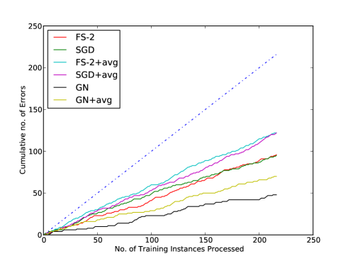
Figure 1: Cumulative training errors on the heart dataset.

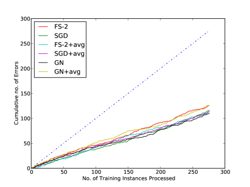
Figure 2: Cumulative training errors on the liver dataset.

To study the behavior of the different learning algorithms during train time, we compute the cumulative number of errors. Cumulative number of errors represents the total misclassification errors encountered up to the current train instance. In an one-pass online learning setting, we must continuously both train as well as apply the trained classifier to classify new instances on the fly. Therefore, a method that obtains a lower number of cumulative errors is desirable. To compare the different methods described in the paper, we plot the cumulative number of errors against the total number of training instances encountered as shown in Figures 1 and 2, respectively for heart and liver datasets. During training, we use the weight vector (or the averaged weight vector for the +avg methods) to classify the current training instances and if it is misclassified by the current model, then it is counted as an error. The 45 degree line in each plot corresponds to the situation where all instances encountered during training are misclassified. All algorithms must lie below this line. To avoid cluttering, we only show the cumulative number of error curves for the following six methods: FS-2, FS-2+avg, SGD, SGD+avg, GN, and GN+avg. Overall, we see that the unsupervised dynamic feature scaling methods GN and GN+avg stand out among the others and report lower numbers of cumulative errors.

7 Conclusion

We studied the problem of feature scaling in one-pass online learning (OPOL) of binary linear classifiers. In OPOL, a learner is allowed to traverse a dataset only once. We presented both supervised as well as unsupervised approaches to dynamically scale feature under the OPOL setting. We evaluated $18$ different learning methods using three popular datasets. Our experimental results show that the unsupervised approach significantly outperforms the supervised approaches and improves the classification accuracy in a state-of-the-art online learning algorithm proposed by [6]. Among the several variants of the supervised feature scaling approach we evaluated, the convex formulation performed best. In future, we plan to explore other forms of feature scaling functions and their effectiveness in numerous online learning algorithms proposed for classification.

References

- [1] Yoshua Bengio, Jerome Louradour, Ronan Collobert, and Jason Weston. Curriculum learning. In ICML’09, pages 41 – 48, 2009.
- [2] Dimitri P. Bertsekas. Incremental gradient, subgradient, and proximal methods for convex optimization: A survey. Technical Report LIDS 2848, MIT, 2010.
- [3] Christopher M. Bishop. Pattern Recognition and Machine Learning. Springer, 2006.
- [4] Tony F. Chan, Gene H. Golub, and Randall J. LeVeque. Algorithms for computing the sample variance: Analysis and recommendations. The American Statistician, 37:242 – 247, 1983.
- [5] Michael Collins. Discriminative training methods for hidden markov models: theory and experiments with perceptron algorithms. In EMNLP’02, pages 1 – 8, 2002.
- [6] Koby Crammer, Ofer Dekel, Joseph Keshet, Shai Shalev-Shwartz, and Yoram Singer. Online passive-aggressive algorithms. Journal of Machine Learning Research, 7:551–585, 2006.
- [7] Koby Crammer, Mark Dredze, and Alex Kulesza. Multi-class confidence weighted algorithms. In EMNLP 2009, pages 496 – 504, 2009.
- [8] Koby Crammer, Mark Dredze, and Fernando Pereira. Exact convex confidence-weighted learning. In NIPS’08, 2008.
- [9] Mark Dredze and Koby Crammer. Active learning with confidence. In ACL’08, pages 233 – 236, 2008.
- [10] Mark Dredze, Koby Crammer, and Fernando Pereira. Confidence-weighted linear classification. In ICML’08, pages 264 – 271, 2008.
- [11] Mark Dredze, Tim Oates, and Christine Piatko. We’re not in kansas anymore: Detecting domain changes in streams. In EMNLP’10, pages 585 – 595, 2010.
- [12] John Duchi, Elad Hazan, and Yoram Singer. Adaptive subgradient methods for online learning and stochastic optimization. In COLT’10, 2010.
- [13] John C. Duchi, Alekh Agrawal, and Martin J. Wainwright. Distributed dual averaging in networks. In NIPS’10, 2010.
- [14] Siddharth Gopal and Yiming Yang. Distributed training of large-scale logistic models. In ICML’13, 2013.
- [15] Long Jiang, Mo Yu, Ming Zhou, Xiaohua Liu, and Tiejun Zhao. Target-dependent twitter sentiment classification. In ACL’11, pages 151 – 160, 2011.
- [16] Robert F. Ling. Comparison of several algorithms for computing sample means and variances. Journal of the American Statistical Association, 69(348):859 – 866, 1974.
- [17] Chao Liu, Hung chih Yang, Jinliang Fan, Li wei He, and Yi-Min Wang. Distributed nonnegative matrix factorization for web-scale dyadic data analysis on mapreduce. In WWW 2010, pages 681–690, 2010.
- [18] Justin Ma, Alex Kulesza, Mark Dredze, Koby Crammer, Lawrence K. Saul, and Fernando Pereira. Exploiting feature covariance in high-dimensional online learning. In AISTAT’10, 2010.
- [19] Omid Madani and Jian Huang. Large-scale many-class prediction via flat techniques. In Large-Scale Hierarchical Classification Workshop of ECIR, 2010.
- [20] Avihai Mejer and Koby Crammer. Confidence in structured-prediction using confidence-weighted models. In EMNLP’10, pages 971 – 981, 2010.
- [21] Avihai Mejer and Koby Crammer. Confidence estimation in structured prediction. Technical Report 798, Center for Communication and Information Technologies, 2011.
- [22] Patrick Pantel, Thomas Lin, and Michael Gamon. Mining entity types from query logs via user intent modeling. In Proceedings of the 50th Annual Meeting of the Association for Computational Linguistics (Volume 1: Long Papers), pages 563–571, Jeju Island, Korea, July 2012. Association for Computational Linguistics.
- [23] Guoqiang Peter Zhang. Neural networks for classification: A survey. IEEE Transactions on System, Man and Cybernetics - Part C, 30(4):451 – 462, November 2000.
- [24] Peilin Zhao and Steven C. H. Hoi. Otl: A framework of online transfer learning. In ICML 2011, 2011.