Gravitational field of a Schwarzschild black hole and a rotating mass ring

Abstract

The linear perturbation of the Kerr black hole has been discussed by using the Newman–Penrose and the perturbed Weyl scalars, $\psi_{0}$ and $\psi_{4}$ can be obtained from the Teukolsky equation. In order to obtain the other Weyl scalars and the perturbed metric, a formalism was proposed by Chrzanowski and by Cohen and Kegeles (CCK) to construct these quantities in a radiation gauge via the Hertz potential. As a simple example of the construction of the perturbed gravitational field with this formalism, we consider the gravitational field produced by a rotating circular ring around a Schwarzschild black hole. In the CCK method, the metric is constructed in a radiation gauge via the Hertz potential, which is obtained from the solution of the Teukolsky equation. Since the solutions $\psi_{0}$ and $\psi_{4}$ of the Teukolsky equations are spin-2 quantities, the Hertz potential is determined up to its monopole and dipole modes. Without these lower modes, the constructed metric and Newman–Penrose Weyl scalars have unphysical jumps on the spherical surface at the radius of the ring. We find that the jumps of the imaginary parts of the Weyl scalars are cancelled when we add the angular momentum perturbation to the Hertz potential. Finally, by adding the mass perturbation and choosing the parameters which are related to the gauge freedom, we obtain the perturbed gravitational field which is smooth except on the equatorial plane outside the ring. We discuss the implication of these results to the problem of the computation of the gravitational self-force to the point particles in a radiation gauge.

I Introduction

The black hole perturbation theory has been a powerful tool to investigate the stability of the black hole, the quasi-normal modes, and the gravitational waves produced by matters such like compact starts orbiting around the hole, and so on. For the Schwarzschild case, the first order metric perturbation is described by the Regge–Wheeler–Zerilli formalism RW1957 ; Z1970 , which relies on the spherical symmetry of the black hole space-time. The Regge–Wheeler and the Zerilli equation are the single, decoupled equation for the odd and even parity modes, respectively, and the master equations are reduced to radial ordinary differential equations by using the Fourier-harmonic expansion. On the other hand, for the Kerr case, it is well-known that there is no such a formalism for the metric perturbation. Instead, the perturbation of the Weyl scalars, $\psi_{0}$ and $\psi_{4}$, are described by the Teukolksy equation with the spin-weight $s=\pm 2$. One method to compute the metric perturbation of Kerr space-time is to solve the coupled partial differential equations numerically. The other method is to construct the metric perturbation from the perturbation of $\psi_{0}$ and $\psi_{4}$ obtained from the Teukolsky equation. Such a method was proposed first by Chrzanowski c and Cohen and Kegeles kc ; ck (See also wald1978 ; Stewart1979 ), and thus is called the CCK formalism. In this method, a radiation gauge is used to calculate the metric perturbation. After these works, however, there were very little development of the CCK formalism for a long time.

New developments were started about a decade ago by Lousto and Whiting LoustoWhiting and Ori ori03 . These were motivated by the necessity to compute the gravitational self-force on the point particle orbiting around a Kerr black hole. Such situations are called EMRI (extreme mass ratio inspiral), and are one of the most important sources of the gravitational wave for the future space laser interferometers such as eLISA eLISA , DECIGO SNK ; DECIGO and BBO BBO .

A first explicit computation of the metric perturbation by using the CCK formalism was done by Yunes and Gonz$\acute{\rm a}$lez YunesGonzalez in which the vacuum perturbation was considered. Keidl, Friedman, and Wiseman kfw were the first to find the explicit metric perturbation produced by a point particle, using the CCK formalism. They considered a system which consists of a Schwarzschild black hole and a static point mass, as a toy model. The metric perturbation is obtained straightforwardly for the multipole modes of $l\geq 2$. They obtained lower modes of $l=0,1$ by considering the regularity of the metric. A singularity, however, remained along a radial line which connect the position of the particle and either the infinity or the black hole horizon. The presence of the singularity was previously discussed by Wald wald1973 and by Barack and Ori BarackOri2001 .

Keidl, Shah, Friedman, Kim and Price ksf+10 ; skf+11 ; sfk12 further developed the formalism to calculate the self-force by using the CCK formalism. In sfk12 , they reported the numerical corrections of gauge invariants of a particle in circular orbit around a Kerr black hole. For the calculation of the gravitational self-force on the particle, it is important to complete the metric perturbation by adding the lower modes in an appropriate gauge. The $l\geq 2$ modes are calculated in a radiation gauge, and the effects of lower modes are added in, what they call, the Kerr gauge.

Recently, Pound, Merlin, and Barack pmb discussed prescriptions for calculating the self-force from completed metric perturbations. With this prescription, once we obtain the metric perturbation which is constructed using a radiation gauge and completed with lower modes appropriately, it is possible to transform its gauge into a local Lorenz gauge. The regularized self-force can then be calculated by using the standard mode-sum method.

In this paper, we consider the metric perturbation of a rotating circular mass ring around a Schwarzschild black hole, in order to understand the problems in constructing the metric perturbation by using the CCK formalism. Especially, we discuss the problem of the completion of the metric perturbation with lower multipole modes. Of course, this is a first step toward the calculation of the metric perturbation produced by a orbiting particle. But this problem is simpler than that of an orbiting particle, since the ring is circular and rotates with a constant angular velocity, and the problem becomes stationary and axisymmetric. Nevertheless, this problem is more complicated than kfw in that both the mass and angular momentum perturbation are involved.

This paper is organized as follows. The first step is to obtain the perturbed Weyl scalars $\psi_{0}$ and $\psi_{4}$ by solving the Teukolsky equation which is discussed in Section II. Next in Section III.1, we describe the CCK formalism in a general form. In Section III.2, the Hertz potential is obtained from $\psi_{0}$ and $\psi_{4}$. In Section III.3, we briefly discuss the gravitational fields computed from the Hertz potential which contains only $l\geq 2$ modes, and show the presence of the singularities in the gravitational fields. In Section III.4, we obtain the Hertz potential of $l=0,1$ modes by considering the continuity of the gravitational field, and obtain the metric perturbation from the completed Hertz potential. Section IV is devoted to summary and discussion.

II Solutions of the Teukolsky equation

In this section we analytically derive $\psi_{0}$ and $\psi_{4}$. The details of the derivation are given in Appendix A and B. Here, we only give the outline and the main results which are used in the subsequent sections.

The Schwarzschild metric is given as

$$\begin{split}\mathrm{d}s^{2}=-\frac{\Delta}{r^{2}}\mathrm{d}t^{2}+\frac{r^{2}}{\Delta}\mathrm{d}r^{2}+r^{2}(\mathrm{d}\theta^{2}+\sin^{2}\theta\mathrm{d}\phi^{2})~{},\end{split}$$ (2.1)

where $\Delta=r^{2}-2Mr$ . Five complex Weyl scalars are defined as

$$\begin{split}&\Psi_{0}=+C_{abcd}l^{a}m^{b}l^{c}m^{d}~{},\\ &\Psi_{1}=+C_{abcd}l^{a}{n}^{b}l^{c}{m}^{d}~{},\\ &\Psi_{2}=+C_{abcd}l^{a}m^{b}\overline{m}^{c}n^{d}~{},\\ &\Psi_{3}=+C_{abcd}l^{a}n^{b}\overline{m}^{c}n^{d}~{},\\ &\Psi_{4}=+C_{abcd}n^{a}\overline{m}^{b}n^{c}\overline{m}^{d}~{},\end{split}$$ (2.2)

where $C_{abcd}$ is the Weyl tensor, and Here, $l^{a},{n}^{b},{m}^{d}$ are the Kinnersley tetrad defined in Appendix A. The overline $\overline{m}$ denotes the complex conjugate of $m$. Note that we adopt the $-$$+$$+$$+$ signature which is different from that of Newman and Penrose np62 and Teukolsky teu . Because of it, although the sign of above Weyl scalars are opposite from those by Newman and Penrose np62 and Teukolsky teu , the Teukolsky equations are left unchanged. In the case of Schwarzschild metric, nonzero Weyl scalar is $\Psi_{2}$.

$$\Psi_{2}=-\frac{M}{r^{3}}~{}.$$ (2.3)

The corresponding perturbed Weyl scalars are denoted by $\psi_{0},~{}\psi_{1},\ldots,~{}\psi_{4}$.

We consider the perturbation of the Schwarzschild metric induced by a rotating ring which is composed by a set of point masses in a circular, geodesic orbit on the equatorial plane. The energy-momentum tensor of the ring is written as

$$\begin{split}T^{ab}=&\int\mathrm{d}{\phi^{\prime}}\frac{mu^{a}u^{b}}{u^{t}r_{0}{}^{2}}\delta(r-r_{0})\delta(\cos\theta)\delta(\phi-\phi^{\prime})\\ =&\frac{mu^{a}u^{b}}{u^{t}r_{0}{}^{2}}\delta(r-r_{0})\delta(\cos\theta)~{},\end{split}$$ (2.4)

where $r_{0}$ is the radius of the ring, and $u^{a}=u^{t}\left((\partial_{t})^{a}+\Omega(\partial_{\phi})^{a}\right)$ is the four-velocity of the ring. The angular velocity $\Omega$ and $u^{t}$ are given as

$$\Omega=\sqrt{\frac{M}{r_{0}{}^{3}}}~{},~{}~{}~{}~{}u^{t}=\sqrt{\frac{r_{0}}{r_{0}-3M}}~{}.$$ (2.5)

The rest mass of the ring becomes $2\pi m~{}(\ll M)$.

Since our perturbed space-time is independent from $t$ and $\phi$, it is sufficient to consider the case of $\omega=0$ and the $m=0$ mode of the spin-weighted spherical harmonics ${}_{s}Y_{lm}(\theta,\phi)$. We expand $\psi_{0}$ as

$$\begin{split}&\psi_{0}(r,\theta)=\sum_{l=2}^{\infty}R^{(2)}_{l}(r)~{}{}_{2}Y_{l}(\theta)~{}.\end{split}$$ (2.6)

The Teukolsky equation for $\psi_{0}$ is given as

$$\begin{split}\left[\frac{1}{r^{2}\Delta^{2}}\frac{\mathrm{d}{}}{\mathrm{d}{r}}\left(\Delta^{3}\frac{\mathrm{d}{}}{\mathrm{d}{r}}\right)-\frac{(l-2)(l+3)}{r^{2}}\right]R^{(2)}_{l}=-4\pi T^{(2)}_{l}~{}{.}\end{split}$$ (2.7)

We also expand $\psi_{4}$ as

$$\begin{split}&\rho^{-4}\psi_{4}(r,\theta)=\sum_{l=2}^{\infty}R^{(-2)}_{l}(r)~{}{}_{-2}Y_{l}(\theta)~{}.\end{split}$$ (2.8)

The Teukolsky equation for $\psi_{4}$ is given as

$$\begin{split}\left[\frac{\Delta^{2}}{r^{2}}\frac{\mathrm{d}{}}{\mathrm{d}{r}}\left(\frac{1}{\Delta}\frac{\mathrm{d}{}}{\mathrm{d}{r}}\right)-\frac{(l+2)(l-1)}{r^{2}}\right]R^{(-2)}_{l}=-4\pi T^{(-2)}_{l}~{}{.}\end{split}$$ (2.9)

Here we defined ${}_{s}Y_{l}(\theta)$ as

$${}_{s}Y_{l}(\theta)\equiv{}_{s}Y_{l0}(\theta,0)~{}.$$ (2.10)

The source terms $T^{(2)}_{l}$ and $T^{(-2)}_{l}$ are given as

$$\begin{split}T^{(2)}_{l}=+2\pi&\frac{1}{r^{4}}{mu^{t}r_{0}{}^{2}}\frac{1}{r^{2}}\delta(r-r_{0})\\ &\times\sqrt{(l+2)(l-1)(l+1)l}~{}{}_{0}Y_{l}(\pi/2)\\ -2i\cdot 2\pi&\frac{1}{r^{4}}{mu^{t}\Omega r_{0}{}^{3}}\frac{\partial{}}{\partial{r}}\frac{1}{r}\delta(r-r_{0})\\ &\times\sqrt{(l+2)(l-1)}{}_{1}Y_{l}(\pi/2)\\ -2\pi&\frac{1}{r^{4}}{mu^{t}\Omega^{2}r_{0}{}^{4}}r^{2}\frac{\partial{}}{\partial{r}}\frac{1}{r^{2}}\frac{\partial{}}{\partial{r}}\delta(r-r_{0})\\ &\times{}_{2}Y_{l}(\pi/2)~{},\end{split}$$ (2.11)

$$\begin{split}T^{(-2)}_{l}=+2\pi&\frac{\Delta^{2}}{4r^{4}}{mu^{t}r_{0}{}^{2}}\frac{1}{r^{2}}\delta(r-r_{0})\\ &\times\sqrt{(l+2)(l-1)(l+1)l}~{}{}_{0}Y_{l}(\pi/2)\\ +2i\cdot 2\pi&\frac{\Delta^{2}}{4r^{4}}{mu^{t}\Omega r_{0}{}^{3}}\frac{\partial{}}{\partial{r}}\frac{1}{r}\delta(r-r_{0})\\ &\times\sqrt{(l+2)(l-1)}{}_{-1}Y_{l}(\pi/2)\\ -2\pi&\frac{\Delta^{2}}{4r^{4}}{mu^{t}\Omega^{2}r_{0}{}^{4}}r^{2}\frac{\partial{}}{\partial{r}}\frac{1}{r^{2}}\frac{\partial{}}{\partial{r}}\delta(r-r_{0})\\ &\times{}_{-2}Y_{l}(\pi/2)~{}.\end{split}$$ (2.12)

A simple relation $\frac{\Delta^{2}}{4}T^{(2)}_{l}(r)=T^{(-2)}_{l}(r)$ holds because of the symmetries.

The Teukolsky equations for $\psi_{0}$ and $\psi_{4}$ above are solved by using the Green’s function, and we obtain

$$\begin{split}R_{l}^{(2)}=&+\frac{4}{M\Delta}\frac{4\pi^{2}mu^{t}~{}{}_{0}Y_{l}(\pi/2)}{\sqrt{(l+2)(l+1)l(l-1)}}\\ &~{}~{}~{}\times\left(-\frac{\Delta_{0}}{2r_{0}{}^{2}}P_{l}^{2}\left(x_{0}^{<}\right)Q_{l}^{2}\left(x_{0}^{>}\right)\right)\\ &-i\frac{4}{M\Delta}\frac{8\pi^{2}mu^{t}\Omega r_{0}{}^{2}~{}{}_{-1}Y_{l}(\pi/2)}{\sqrt{(l+2)(l-1)}(l+1)l}\\ &~{}~{}~{}\times\left(-\frac{\mathrm{d}{}}{\mathrm{d}{r_{0}}}\frac{\Delta_{0}}{2r_{0}{}^{2}}P_{l}^{2}\left(x_{0}^{<}\right)Q_{l}^{2}\left(x_{0}^{>}\right)\right)\\ &-\frac{4}{M\Delta}\frac{4\pi^{2}mu^{t}\Omega^{2}r_{0}{}^{4}{}_{-2}Y_{l}(\pi/2)}{{(l+2)(l-1)(l+1)l}}\\ &~{}~{}~{}\times\left(-\frac{\mathrm{d}{}}{\mathrm{d}{r_{0}}}\frac{1}{r_{0}{}^{2}}\frac{\mathrm{d}{}}{\mathrm{d}{r_{0}}}r_{0}{}^{2}\frac{\Delta_{0}}{2r_{0}{}^{2}}P_{l}^{2}\left(x_{0}^{<}\right)Q_{l}^{2}\left(x_{0}^{>}\right)\right)~{},\end{split}$$ (2.13)

$$\begin{split}R_{l}^{(-2)}=&+\frac{\Delta}{M}\frac{4\pi^{2}mu^{t}~{}{}_{0}Y_{l}(\pi/2)}{\sqrt{(l+2)(l+1)l(l-1)}}\\ &~{}~{}~{}\times\left(-\frac{\Delta_{0}}{2r_{0}{}^{2}}P_{l}^{2}\left(x_{0}^{<}\right)Q_{l}^{2}\left(x_{0}^{>}\right)\right)\\ &-i\frac{\Delta}{M}\frac{8\pi^{2}mu^{t}\Omega r_{0}{}^{2}~{}{}_{-1}Y_{l}(\pi/2)}{\sqrt{(l+2)(l-1)}(l+1)l}\\ &~{}~{}~{}\times\left(-\frac{\mathrm{d}{}}{\mathrm{d}{r_{0}}}\frac{\Delta_{0}}{2r_{0}{}^{2}}P_{l}^{2}\left(x_{0}^{<}\right)Q_{l}^{2}\left(x_{0}^{>}\right)\right)\\ &-\frac{\Delta}{M}\frac{4\pi^{2}mu^{t}\Omega^{2}r_{0}{}^{4}{}_{-2}Y_{l}(\pi/2)}{{(l+2)(l-1)(l+1)l}}\\ &~{}~{}~{}\times\left(-\frac{\mathrm{d}{}}{\mathrm{d}{r_{0}}}\frac{1}{r_{0}{}^{2}}\frac{\mathrm{d}{}}{\mathrm{d}{r_{0}}}r_{0}{}^{2}\frac{\Delta_{0}}{2r_{0}{}^{2}}P_{l}^{2}\left(x_{0}^{<}\right)Q_{l}^{2}\left(x_{0}^{>}\right)\right)~{},\end{split}$$ (2.14)

where

$${\Delta_{0}\equiv r_{0}{}^{2}-2Mr_{0}~{},}$$ (2.15)

$$x_{0}^{<}\equiv\frac{{\rm min}(r,r_{0})-M}{M}~{},~{}~{}~{}~{}~{}x_{0}^{>}\equiv\frac{{\rm max}(r,r_{0})-M}{M}~{}.$$ (2.16)

These two radial functions are related as $\frac{\Delta^{2}}{4}R_{l}^{(2)}(r)=R_{l}^{(-2)}(r)$. With this relation, together with the fact ${}_{2}Y_{l}(\theta)={}_{-2}Y_{l}(\theta)$, we find that $\psi_{0}$ and $\psi_{4}$ are related in a very simple equation,

$$\psi_{4}=\frac{\Delta^{2}}{4r^{4}}\psi_{0}~{}.$$ (2.17)

Note that this relation holds because of the symmetries of our space-time.

We also find that because the matter is present on the equatorial plane, and ${}_{s}Y_{l}(\theta)$ is evaluated only at $\theta=\pi/2$, we have

$${\rm Re}\left(R_{l}^{(\pm 2)}(r)\right)=0~{}~{}~{}{\rm for}~{}{\rm odd}~{}l{~{},}$$

and

$${\rm Im}\left(R_{l}^{(\pm 2)}(r)\right)=0~{}~{}~{}{\rm for}~{}{\rm even}~{}l{~{}.}$$

Therefore, the real part of $\psi_{0}$ and $\psi_{4}$ is symmetric about the equatorial plane and the imaginary part is antisymmetric.

$$\begin{split}&{\rm Re}(\psi_{0/4}(r,\pi-\theta))={\rm Re}(\psi_{0/4}(r,\theta))~{},\\ &{\rm Im}(\psi_{0/4}(r,\pi-\theta))=-{\rm Im}(\psi_{0/4}(r,\theta))~{}.\end{split}$$ (2.18)

In Fig. 1, We show the radial dependence of $\psi_{0}$ and $\psi_{4}$, with fixed angular coordinate $\theta=\pi/4$. Note that $\psi_{0}$ and $\psi_{4}$ are smooth at the sphere, $r=r_{0}$, except for $\theta=\pi/2$, where the energy-momentum tensor vanishes.

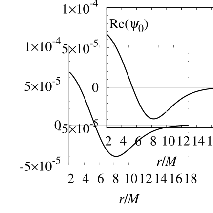
Figure 1: Radial dependence of $\psi_{0}$ and $\psi_{4}$ obtained by solving the Teukolsky equation. The real parts of $\psi_{0}(r,\theta=\pi/4)$ (top left) and $\psi_{4}(r,\theta=\pi/4)$ (top right), and the imaginary parts of $\psi_{0}(r,\theta=\pi/4)$ (bottom left) and $\psi_{4}(r,\theta=\pi/4)$ (bottom right) are shown. The radius of the ring is $r_{0}=10M$, and $m=M/100$. We see the smoothness at $r=r_{0}$.

III Construction of the perturbed gravitational fields

Chrzanowski c and Cohen and Kegeles kc introduced a formalism to compute the perturbed metric in a “radiation gauge” from Teukolsky valuables $\psi_{0}$ and $\psi_{4}$. In this section, we describe how we can use the CCK formalism to calculate the perturbed gravitational fields produced by the rotating ring.

III.1 The CCK formalism

In the CCK formalism, the Hertz potential $\Psi$, which is a solution of the homogeneous Teukolsky equation, is introduced. The perturbed metric is obtained by differentiating the Hertz potential. In order to obtain the relation between the Hertz potential and the perturbed metric, two kinds of gauge conditions are used. They are called “Ingoing Radiation Gauge” (IRG) and “Outgoing Radiation Gauge” (ORG). The IRG is defined by the conditions $h_{ab}l^{b}=h^{a}{}_{a}=0$. The perturbed metric $h_{ab}$ in IRG is related to the Hertz potential as

$$\begin{split}h_{ab}&=-\big{[}l_{a}l_{b}(\overline{\boldsymbol{\delta}}+2\beta)(\overline{\boldsymbol{\delta}}+4\beta)\overline{\Psi}\\ &~{}~{}~{}~{}~{}-2l_{(a}\overline{m}_{b)}(\boldsymbol{D}+\rho)(\overline{\boldsymbol{\delta}}+4\beta)\overline{\Psi}\\ &~{}~{}~{}~{}~{}~{}~{}~{}~{}~{}+\overline{m}_{a}\overline{m}_{b}(\boldsymbol{D}-\rho)(\boldsymbol{D}+3\rho)\overline{\Psi}\big{]}\\ &~{}~{}~{}+\left[{\rm c.c.}\right]~{},\end{split}$$ (3.1)

where $\left[{\rm c.c.}\right]$ represents the complex conjugate of the first term. The bold greek characters are derivative operators associated with the tetrad defined in Appendix A. The Hertz potential $\Psi$ in IRG satisfies the source-free Teukolsky equation with $s=-2$.

$$(\boldsymbol{\Delta}+\mu+2\gamma)({\boldsymbol{D}}+3\rho)\Psi-3\Psi_{2}\Psi=(\overline{\boldsymbol{\delta}}-2\beta)({\boldsymbol{\delta}}+4\beta)\Psi~{}.$$ (3.2)

Equivalently, this equation is written as

$$(\boldsymbol{\Delta}-2\mu+2\gamma)\boldsymbol{D}\Psi+3\rho\partial_{t}\Psi=(\overline{\boldsymbol{\delta}}-2\beta)(\boldsymbol{\delta}+4\beta)\Psi~{}.$$ (3.3)

By using (3.1) and (3.2), the relations between the perturbed Weyl scalars and the Hertz potential are obtained as ref:KFWtypo

$$\psi_{0} =\frac{1}{2}\boldsymbol{D}^{4}\overline{\Psi}~{},$$ (3.4a)

$$\psi_{1} =\frac{1}{2}\boldsymbol{D}^{3}(\overline{\boldsymbol{\delta}}+4\beta)\overline{\Psi}~{},$$ (3.4b)

$$\psi_{2} =\frac{1}{2}\boldsymbol{D}^{2}(\overline{\boldsymbol{\delta}}+2\beta)(\overline{\boldsymbol{\delta}}+4\beta)\overline{\Psi}~{},$$ (3.4c)

$$\psi_{3} =\frac{1}{2}\boldsymbol{D}\overline{\boldsymbol{\delta}}(\overline{\boldsymbol{\delta}}+2\beta)(\overline{\boldsymbol{\delta}}+4\beta)\overline{\Psi}+3\gamma\boldsymbol{D}\rho(\boldsymbol{\delta}+4\beta)\Psi~{},$$ (3.4d)

$$\psi_{4} =\frac{1}{2}(\overline{\boldsymbol{\delta}}-2\beta)\overline{\boldsymbol{\delta}}(\overline{\boldsymbol{\delta}}+2\beta)(\overline{\boldsymbol{\delta}}+4\beta)\overline{\Psi}-3\gamma\rho^{2}\partial_{t}\Psi~{}.$$ (3.4e)

On the other hand, ORG is defined by the conditions $h_{ab}n^{b}=h^{a}{}_{a}=0$. The perturbed metric $h_{ab}^{\rm ORG}$ is related to the Hertz potential as

$$\begin{split}h_{ab}^{\rm ORG}&=-\Big{[}n_{a}n_{b}\left(-\frac{2r^{2}}{\Delta}\right)^{2}(\overline{\boldsymbol{\delta}}+2\beta)(\overline{\boldsymbol{\delta}}+4\beta)\frac{\Delta^{2}}{4}{\Psi}\\ &~{}~{}~{}~{}~{}-2n_{(a}\overline{m}_{b)}\left(-\frac{2r^{2}}{\Delta}\right)(\boldsymbol{D}+\rho)(\overline{\boldsymbol{\delta}}+4\beta)\frac{\Delta^{2}}{4}{\Psi}\\ &~{}~{}~{}~{}~{}~{}~{}~{}~{}~{}+\overline{m}_{a}\overline{m}_{b}(\boldsymbol{D}-\rho)(\boldsymbol{D}+3\rho)\frac{\Delta^{2}}{4}{\Psi}\Big{]}\\ &~{}~{}~{}+\left[{\rm c.c.}\right]~{}.\end{split}$$ (3.5)

The Hertz potential $\Psi$ in ORG satisfies the source-free Teukolsky equation with $s=2$.

$$\begin{split}(\tilde{\boldsymbol{\Delta}}+\mu+2\gamma)&(\tilde{\boldsymbol{D}}+3\rho)\frac{\Delta^{2}}{4}\Psi-3\Psi_{2}\frac{\Delta^{2}}{4}\Psi\\ &~{}~{}~{}~{}~{}=(\boldsymbol{\delta}-2\beta)(\overline{\boldsymbol{\delta}}+4\beta)\frac{\Delta^{2}}{4}\Psi~{}.\end{split}$$ (3.6)

Equivalently, this equation is written as

$$\begin{split}(\tilde{\boldsymbol{\Delta}}-2\mu+2\gamma)\tilde{\boldsymbol{D}}\frac{\Delta^{2}}{4}\Psi&-3\rho\partial_{t}\frac{\Delta^{2}}{4}\Psi\\ &=(\boldsymbol{\delta}-2\beta)(\overline{\boldsymbol{\delta}}+4\beta)\frac{\Delta^{2}}{4}\Psi~{}.\end{split}$$ (3.7)

By using (3.5) and (3.6), the relations between the perturbed Weyl scalars and the Hertz potential are obtained as

$$\left(-\frac{2r^{2}}{\Delta}\right)^{2}\psi_{4} =\frac{1}{2}\boldsymbol{D}^{4}\frac{\Delta^{2}}{4}\overline{\Psi}~{},$$ (3.8a)

$$\left(-\frac{2r^{2}}{\Delta}\right)\psi_{3} =\frac{1}{2}\boldsymbol{D}^{3}(\overline{\boldsymbol{\delta}}+4\beta)\frac{\Delta^{2}}{4}\overline{\Psi}~{},$$ (3.8b)

$$\psi_{2} =\frac{1}{2}\boldsymbol{D}^{2}(\overline{\boldsymbol{\delta}}+2\beta)(\overline{\boldsymbol{\delta}}+4\beta)\frac{\Delta^{2}}{4}\overline{\Psi}~{},$$ (3.8c)

$$\left(-\frac{\Delta}{2r^{2}}\right)\psi_{1} =\frac{1}{2}\boldsymbol{D}\overline{\boldsymbol{\delta}}(\overline{\boldsymbol{\delta}}+2\beta)(\overline{\boldsymbol{\delta}}+4\beta)\frac{\Delta^{2}}{4}\overline{\Psi}$$

$$~{}~{}~{}~{}~{}~{}~{}~{}~{}~{}+3\gamma\boldsymbol{D}\rho(\boldsymbol{\delta}+4\beta)\frac{\Delta^{2}}{4}\Psi~{},$$ (3.8d)

$$\left(-\frac{\Delta}{2r^{2}}\right)^{2}\psi_{0} =\frac{1}{2}({\boldsymbol{\delta}}-2\beta){\boldsymbol{\delta}}({\boldsymbol{\delta}}+2\beta)({\boldsymbol{\delta}}+4\beta)\frac{\Delta^{2}}{4}\overline{\Psi}$$

$$~{}~{}~{}~{}~{}~{}~{}~{}~{}~{}+3\gamma\rho^{2}\partial_{t}\frac{\Delta^{2}}{4}\Psi~{}.$$ (3.8e)

Whichever gauge we choose, we look for the Hertz potential that satisfies the relations to $\psi_{0}$ and $\psi_{4}$, Eqs. (3.4a) and (3.4e), or Eqs. (3.8a) and (3.8e).

III.2 The Hertz potential and the metric perturbation in IRG

In this paper, we use IRG to construct the perturbed gravitational fields. From (3.4), the relations between Teukolsky valuables and the Hertz potential become

$$\psi_{0}=\frac{1}{2}\left(\frac{\partial}{\partial r}\right)^{4}\overline{\Psi}~{},$$ (3.9)

$$\psi_{4}=\frac{1}{2}\frac{1}{4r^{4}}\sin^{2}\theta\left(\frac{\partial}{\partial\cos\theta}\right)^{4}\sin^{2}\theta\overline{\Psi}~{}.$$ (3.10)

Here, we used the fact that the ring and the black hole are stationary and axisymmetric.

Our task is to find Hertz potential which satisfies (3.9), (3.10) and (3.3).

By substituting the solution of the Teukolsky equation,

$$\psi_{4}=\frac{1}{r^{4}}\sum_{l=2}^{\infty}R_{l}^{(-2)}(r)_{-2}Y_{l}(\theta)$$

into (3.10), we obtain

$$\sum_{l=2}^{\infty}8R_{l}^{(-2)}\frac{{}_{-2}Y_{l}(\theta)}{\sin^{2}\theta}=\left(\frac{\partial}{\partial\cos\theta}\right)^{4}\sin^{2}\theta\overline{\Psi}~{}{.}$$ (3.11)

From (A.24), we can obtain the following relation

$$\left(\frac{\partial}{\partial\cos\theta}\right)^{4}\frac{{}_{-2}Y_{l}(\theta)}{\sin^{2}\theta}=\frac{1}{\sin^{2}\theta}\frac{{}_{2}Y_{l}(\theta)}{(l+2)(l-1)(l+1)l}~{}{.}$$ (3.12)

By using this relation, $\Psi$ can be integrated as

$$\begin{split}\overline{\Psi}(r,\theta)&=\overline{\Psi_{\rm P}}+\overline{\Psi_{\rm H}},\end{split}$$ (3.13)

where

$$\overline{\Psi_{\rm P}}\equiv\sum_{l=2}^{\infty}\frac{8{R_{l}^{(-2)}(r)_{2}Y_{l}(\theta)}}{(l+2)(l-1)(l+1)l}~{},$$ (3.14)

$$\begin{split}\overline{\Psi_{\rm H}}&\equiv\frac{2A}{\sin^{2}\theta}\bigg{(}\frac{a(r)}{6}\cos^{3}\theta+\frac{b(r)}{2}\cos^{2}\theta\\ &~{}~{}~{}~{}~{}~{}~{}~{}~{}~{}~{}~{}~{}~{}~{}~{}~{}~{}~{}~{}~{}~{}~{}~{}~{}+c(r)\cos\theta+d(r)\bigg{)}~{},\end{split}$$ (3.15)

and where $\overline{\Psi}$ is the complex conjugate of $\Psi$. $a(r)$, $b(r)$, $c(r)$, and $d(r)$ are arbitrary functions and $A$ is a constant defined as

$$A\equiv\frac{m}{r_{0}\sqrt{\Delta_{0}}}~{}.$$ (3.16)

Here, $\Psi_{\rm P}$ and $\Psi_{\rm H}$ are the particular solution and the homogeneous solution of the equation (3.10), respectively. The particular solution $\Psi_{\rm P}$ satisfies (3.9) and (3.3) in the region, $r\neq r_{0}$. The reason is as follows. From the Teukolsky–Starobinsky relation, we obtain

$$\left(\frac{\partial}{\partial r}\right)^{4}\frac{R_{l}^{(-2)}(r)}{(l+2)(l-1)(l+1)l}=\frac{1}{4}R_{l}^{(2)}(r)~{}{.}$$ (3.17)

By using this, we can obtain $\psi_{0}$ by substituting $\Psi_{\rm P}$ into (3.9). Further, since $R_{l}^{(-2)}(r)$ is the solution of the radial Teukolsky equation with the source term consisting of a circular rotating ring, it satisfies the homogeneous Teukolsky equation in the region, $r\neq r_{0}$. Thus, it is clear that the particular solution $\Psi_{\rm P}$ of the form (3.14) satisfies (3.3) in the region, $r\neq r_{0}$. It is now shown that $\Psi_{\rm P}$ is a Hertz potential that satisfies (3.9), (3.10), and (3.3) everywhere except for the region, $r=r_{0}$.

$\Psi_{\rm P}$ is not only singular at $r=r_{0}$, but also does not include lower modes ($l=0,1$). The monopole perturbation and the dipole perturbation of the space-time are considered to be included in the “homogeneous solution” part $\Psi_{\rm H}$.

We can obtain constraints on the functions $a(r)$, $b(r)$, $c(r)$, and $d(r)$ in $\Psi_{\rm H}$ from (3.3). By substituting $\Psi_{\rm H}$ into (3.3), we obtain

$$(\boldsymbol{\Delta}-2\mu+2\gamma)\boldsymbol{D}\Psi_{\rm H}=(\overline{\boldsymbol{\delta}}-2\beta)(\boldsymbol{\delta}+4\beta)\Psi_{\rm H}~{}.$$ (3.18)

This condition implies that each of $a(r)$, $b(r)$, $c(r)$, and $d(r)$ must be in the following forms.

$$\begin{split}&a(r)=a_{1}r^{2}(r-3M)+a_{2}~{},\\ &b(r)=b_{1}r^{2}+b_{2}(r-M)~{},\\ &c(r)=-\frac{a_{1}}{2}(r^{2}+4M^{2})(r-M)-\frac{a_{2}}{2}\\ &~{}~{}~{}~{}~{}~{}~{}~{}~{}~{}~{}~{}~{}~{}~{}+c_{1}r^{2}+c_{2}(r-M)~{},\\ &d(r)=\frac{b_{1}}{2}r^{2}+\frac{b_{2}}{2}r+d_{1}r^{2}(r-3M)+d_{2}~{}.\end{split}$$ (3.19)

Here $a_{1}$, $a_{2}$, etc. are arbitrary complex constants. Then, the right-hand side of (3.9) vanishes when we substitute $\Psi_{\rm H}$ with constrains (3.19). Thus, $\Psi_{\rm H}$ with (3.19) is a homogeneous solution of (3.9) and (3.10), and satisfies (3.3).

It is known ori03 that the Hertz potential that globally satisfies (3.9), (3.10), and (3.3) simultaneously does not exist because of the presence of matter (the ring). Thus, we need to give up the global regularity of the solution. We find that we can obtain a solution which is smooth at $r=r_{0}$ if we abandon the smoothness of the Hertz potential at $(r\geq r_{0},~{}\theta=\pi/2)$. We also find that in order to obtain the smoothness at $r=r_{0}$, we need to include the contribution from the lower modes ($l=0,1$). We show that this can be done by choosing eight complex parameters, $a_{1}$, $a_{2}$, etc., appropriately, and making the Hertz potential $\Psi=\Psi_{\rm P}+\Psi_{\rm H}$ satisfy (3.9), (3.10), and (3.3) everywhere except for the region $(r\geq r_{0},~{}\theta=\pi/2)$.

III.3 Fields corresponding to $\Psi_{\rm P}$

Figure 2: Radial dependence of the real parts of $\psi_{1}$ (left), $\psi_{2}$ (center), and $\psi_{3}$ (right) derived from $\Psi_{\rm P}$ at $\theta=\pi/4$. The radius of the ring is $r_{0}=10M$. They are discontinuous at $(r=r_{0},~{}\theta=\pi/4)$.

Figure 3: Radial dependence of the imaginary parts of $\psi_{1}$ (left), $\psi_{2}$ (center), and $\psi_{3}$ (right) derived from $\Psi_{\rm P}$ at $\theta=\pi/4$. The radius of the ring is $r_{0}=10M$. They are discontinuous at $(r=r_{0},~{}\theta=\pi/4)$.

Here, we demonstrate the behavior of the Weyl scalars associated with $\Psi_{\rm P}$. We introduce a notation like $\psi_{1}^{\rm P}$ which means that it is calculated by substituting $\Psi=\Psi_{\rm P}$ into the equation for $\psi_{1}$ in (3.4). In Figs. 2 and 3, we show the radial dependence of the real and imaginary parts of $\psi_{1}^{\rm P},\psi_{2}^{\rm P}$ and $\psi_{3}^{\rm P}$ at $\theta=\pi/4$.

As discussed in the previous section, $\psi_{0}^{\rm P}$ agree with the Teukolsky solution $\psi_{0}$, therefore the graph is the same as Fig. 1. Other Weyl scalars, $\psi_{1}^{\rm P}$, $\psi_{2}^{\rm P}$, and $\psi_{3}^{\rm P}$, have discontinuity on the surface of sphere at radius $r=r_{0}$, although there is no matter field on the surface $(r_{0},~{}\theta\neq\pi/2)$. It is also apparent that the perturbed metric $h_{\mu\nu}^{\rm P}$ calculated from $\Psi_{\rm P}$ is not smooth on the surface of the sphere, too.

Figure 4: Radial dependence of the imaginary parts of $\psi_{1}$ (left), $\psi_{2}$ (center), and $\psi_{3}$ (right) derived from $\Psi_{\rm P}+\Psi_{\rm H}$ at $\theta=\pi/4$. The radius of the ring is $r_{0}=10M$. It is clear that they are continuous at $r=r_{0}$.

III.4 $\Psi_{\rm H}$

III.4.1 Contribution of angular momentum perturbation

Keidl, Friedman, and Wiseman (2007) kfw illuminated that some of parameters are physical parameters and others are pure gauge. They found that ${\rm Re}(b_{1})$ and ${\rm Re}(b_{2})$ contribute to the mass perturbation of the space-time and ${\rm Im}(a_{2})$ contributes to the angular momentum perturbation of the space-time. Specifically, it is found that

$$\begin{split}&\delta M=-A(3M{\rm Re}(b_{1})+{\rm Re}(b_{2}))~{},\\ &\delta J=-A{\rm Im}(a_{2})~{}.\end{split}$$ (3.20)

The latter relation is obtained as below kfw . The metric perturbation due to small angular momentum to the Schwarzschild space-time is given in the Boyer–Lindquist coordinates as

$$h_{ab}^{\rm Kerr}=-\frac{4\delta J}{r}\sin^{2}\theta(\mathrm{d}t)_{(a}(\mathrm{d}\phi)_{b)}~{}{.}$$ (3.21)

The corresponding tetrad components are

$$h_{23}^{\rm Kerr}=-i\frac{\delta J}{\sqrt{2}r^{2}}\sin\theta~{},~{}~{}~{}~{}~{}h_{13}^{\rm Kerr}=-i\frac{2\delta J}{\sqrt{2}\Delta}\sin\theta~{}.$$ (3.22)

We can transform these into ingoing radiation gauge, with the gauge vector

$$\xi^{a}=\xi^{3}m^{a}+\xi^{4}\overline{m}^{a};$$

$$\xi^{3}=-\xi^{4}=-\frac{i\delta J}{\sqrt{2}M}\left(1+\frac{r}{2M}\ln\left(1-\frac{2M}{r}\right)\right)~{}.$$ (3.23)

The resultant nonzero component of $h_{ab}=h_{ab}^{\rm Kerr}+\mathcal{L}_{\xi}g_{ab}$ is

$$h_{23}=-i\frac{\sqrt{2}\delta J}{r^{2}}\sin\theta~{}.$$ (3.24)

The metric associated with the imaginary part of $a_{2}$ can be obtained by inserting (3.15) and (3.19) into (3.1), and becomes $h_{23}^{\rm H}=i(\sqrt{2}A{\rm Im}(a_{2})/r^{2})\sin\theta$. We thus obtain $\delta J=-A{\rm Im}(a_{2})$.

In our case, $\delta M$ and $\delta J$ are the energy and angular momentum of the rotating ring, respectively. They are

$$M_{\rm ring}\equiv-2\pi mu_{a}(\partial_{t})^{a}~{},~{}~{}~{}~{}~{}J_{\rm ring}\equiv 2\pi mu_{a}(\partial_{\phi})^{a}~{},$$ (3.25)

where $u^{a}$ is the four-velocity of the ring,

$$u^{a}=\sqrt{\frac{r_{0}}{r_{0}-3M}}\left((\partial_{t})^{a}+\sqrt{\frac{M}{r_{0}{}^{3}}}(\partial_{\phi})^{a}\right)~{}.$$

Interestingly, the jumps of ${\rm Im}(\psi_{1})$, ${\rm Im}(\psi_{2})$, and ${\rm Im}(\psi_{3})$ disappeared when we choose ${\rm Im}(a_{2})=0$ for $r<r_{0}$ and ${\rm Im}(a_{2})=-\delta J/A$ for $r>r_{0}$. Namely, the imaginary parts of $\psi_{1}$, $\psi_{2}$, and $\psi_{3}$ are continuous at $r=r_{0}$ if we choose

$$\Psi=\left\{\begin{array}[]{ll}\Psi_{\rm P},&(2M<r<r_{0}){}\\ \Psi_{\rm P}+\frac{2i\delta J}{\sin^{2}\theta}\left(\frac{1}{6}\cos^{3}\theta-\frac{1}{2}\cos\theta\right).&(r_{0}<r){}\end{array}\right.$$ (3.28)

(3.29)

Further, they also look smooth at $r=r_{0}$ (Fig. 4).

Although we want to determine other parameters in a similar way, we can not do it. One reason is that since the mass perturbation in (3.20) contains two parameters, ${\rm Re}(b_{1})$ and ${\rm Re}(b_{2})$, it is not possible to determine them from only one equation. Further, we don’t have similar equations for other parameters which are not related to the mass and angular momentum perturbation.

III.4.2 Determination of all parameters in $\Psi_{\rm H}$

We now determine all other parameters so that the discontinuity of all the fields at $r=r_{0}$ disappears.

Details are in the appendix. First, we obtain four conditions by demanding that the metric perturbation and the Weyl scalars should not diverge at $\theta=0$ and ${\theta=}\pi$. This can be satisfied when the Hertz potential $\Psi$ does not diverge at $\theta=0$ and $\theta=\pi$. From the condition at $\theta=0$, we obtain

$$\begin{split}&3d_{1}=a_{1}~{},~{}~{}~{}c_{1}=Ma_{1}-b_{1}~{},\\ &c_{2}=2M^{2}a_{1}-b_{2}~{},~{}~{}~{}6d_{2}=2a_{2}-3Mb_{2}~{}{.}\end{split}$$ (3.30)

From the condition at $\theta=\pi$, we obtain

$$\begin{split}&3d_{1}=-a_{1}~{},~{}~{}~{}c_{1}=Ma_{1}+b_{1}~{},\\ &c_{2}=2M^{2}a_{1}+b_{2}~{},~{}~{}~{}6d_{2}=-2a_{2}-3Mb_{2}~{}{.}\end{split}$$ (3.31)

These sets of conditions are simultaneously satisfied if and only if $a_{1}=a_{2}=b_{1}=b_{2}=c_{1}=c_{2}=d_{1}=d_{2}=0$, i.e. $\Psi_{\rm H}=0$. This means that we can not have the contribution from the mass and the angular momentum perturbation. This implies that we can not obtain the regular solution globally. However, we find that if we divide the space-time into several region, we can obtain regular solution in each region. Namely, we divide the region into three regions: $(2M<r<r_{0})$, $(r>r_{0},~{}0\leq\theta<\pi/2)$, and $(r>r_{0},~{}\pi/2<\theta\leq\pi)$. We denote each region by $I$, $N$, and $S$, respectively (Fig. 5).

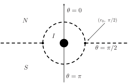
Figure 5: $r$-$\theta$ plane. The three regions are divided by dashed lines. The filled black circle at the center is the region within the event horizon of the black hole. The two black dots represent the position of the ring.

We look for the set of parameters that satisfy (3.30) in $N$ and (3.31) in $S$. Since these are four equations among eight unknown parameters, the remaining parameters we have to determine are four.

As in the case of the contribution of the angular momentum perturbation, (3.29), we add $\Psi_{\rm H}$ only at $r>r_{0}$. Here, we note the symmetry of $\Psi_{\rm P}$. From (3.14), we find that, just like $\psi_{0}$ and $\psi_{4}$, the real and imaginary part of $\Psi_{\rm P}$ are symmetric and antisymmetric about the equatorial plane respectively. In order to kill the jump of $\Psi_{\rm P}$ at $r=r_{0}$, $\Psi_{\rm H}$ at $r>r_{0}$ must have the same symmetry about the equatorial plane. Therefore we get

$$\begin{split}&a_{N}(r)=-\overline{a_{S}}(r)~{},~{}~{}~{}~{}~{}b_{N}(r)=\overline{b_{S}}(r)~{},\\ &c_{N}(r)=-\overline{c_{S}}(r)~{},~{}~{}~{}~{}~{}d_{N}(r)=\overline{d_{S}}(r)~{}.\end{split}$$ (3.32)

Here, $a_{N}(r)$ means $a(r)$ in $N$, and $a_{S}(r)$ means $a(r)$ in $S$, etc. It is sufficient if we determine four complex parameters only in the region $N$ or $S$. From (3.30), we adopt $a_{1}$, $a_{2}$, $b_{1}$ and $b_{2}$ of $\Psi_{\rm H}$ in region $N$ as independent parameters. When the parameters satisfy (3.30), the fields corresponding to $\Psi_{\rm H}$ and $\Psi_{\rm H}$ in $N$ can be written as they include only $a_{1}$, $a_{2}$, $b_{1}$ and $b_{2}$ (equations (D.2)-(D.4)).

We numerically determine values of these parameters that satisfy the continuity conditions

$$\begin{split}\left[F_{\rm P}(r,\theta)\right]_{r_{0}}+F_{\rm H}(r_{0},\theta)=0~{}\end{split}$$

for $F=\psi_{1},~{}\psi_{2},~{}\psi_{3},~{}h_{22},~{}h_{23},~{}h_{33},~{}\Psi$, where

$$\left[F_{\rm P}(r,\theta)\right]_{r_{0}}\equiv\lim_{r\rightarrow r_{0}{}^{+}}F_{\rm P}(r,\theta)-\lim_{r\rightarrow r_{0}{}^{-}}F_{\rm P}(r,\theta)~{}.$$ (3.33)

By using the relations between these four parameters, $a_{1}$, $a_{2}$, $b_{1}$ and $b_{2}$, with $F_{\rm H}$ above given in (D.2)-(D.4), we obtain

$$\begin{split}&(a_{1})_{N}=-0.0000025233-4.2486i~{},\\ &(a_{2})_{N}=-134.33-2123.8i~{},\\ &(b_{1})_{N}=67.169+34.993i~{},\\ &(b_{2})_{N}=-738.86-0.079440i~{}.\\ \end{split}$$

when $M=1~{},m=M/100~{},r_{0}=10M$.

Figure 6: Radial dependence of the real part of $\psi_{1}$ (left), $\psi_{2}$ (center), and $\psi_{3}$ (right) derived from $\Psi_{\rm P}+\Psi_{\rm H}$, with $\theta=\pi/4$ fixed. The radius of the ring is $r_{0}=10M$. It is clear that they are continuous at $r=r_{0}$.

Figure 7: Radial dependence of the each component of $h_{ab}$ derived from $\Psi$ at $\theta=\pi/4$. The radius of the ring is $r_{0}=10M$. They are continuous at $r=r_{0}$.

The plots of ${\rm Re}(\psi_{1})$, ${\rm Re}(\psi_{2})$ and ${\rm Re}(\psi_{3})$ derived from $\Psi_{\rm P}+\Psi_{\rm H}$ are shown in Fig. 6. We find that all of the discontinuity disappeared. Note that because of the relations (3.32), each of parameters ${\rm Re}(b_{1})$, ${\rm Re}(b_{2})$, and ${\rm Im}(a_{2})$ is the same value in $N$ and $S$. Thus, $\delta M$ and $\delta J$ in (3.20) is the same in $N$ and $S$. Interestingly, we numerically obtain the very good agreement between ($\delta M$, $\delta J$) and the mass and angular momentum of the ring, (3.25). We obtain from (3.20),

$$\begin{split}\delta M&=-A(3M{\rm Re}(b_{1})+{\rm Re}(b_{2}))={0.0600781}~{}{,}\\ \delta J&=-A{\rm Im}(a_{2})={0.237451}~{}.\\ \end{split}$$ (3.34)

On the other hand, from (3.25)

$$\begin{split}M_{\rm ring}&={0.06007874270}~{},\\ J_{\rm ring}&={0.2374820823}~{}{.}\\ \end{split}$$ (3.35)

Although the method to determine the $\Psi_{\rm H}$ here is rather heuristic, this excellent agreement suggests the validity of the method and the results. Further discussion on the the accuracy of the numerical results is given at the end of Appendix D.

The results in the case of $r_{0}/M=6,10,20,50$ are shown in Table 1 and 2.

Table 1: $\delta M$

$r_{0}/M$	$\delta M$	$M_{\rm ring}$	$|(M_{\rm ring}-\delta M)/M_{\rm ring}|$
6	0.0592444	0.05923843916	1.008027909 $\times 10^{-4}$
10	0.0600781	0.06007874270	1.005730101 $\times 10^{-5}$
20	0.0613351	0.06133564195	8.821135362 $\times 10^{-6}$
50	0.0622144	0.06221386387	7.995806223 $\times 10^{-6}$
100	0.0625205	0.06252015946	5.948001469 $\times 10^{-6}$

Table 2: $\delta J$

$r_{0}/M$	$\delta J$	$J_{\rm ring}$	$|(J_{\rm ring}-\delta J)/J_{\rm ring}|$
6	0.217649	0.2176559237	3.301954698 $\times 10^{-5}$
10	0.237451	0.2374820823	1.308149216 $\times 10^{-4}$
20	0.304774	0.3047792551	1.758912364 $\times 10^{-5}$
50	0.458263	0.4582483860	3.190540426 $\times 10^{-5}$
100	0.637962	0.6379608107	1.972221458 $\times 10^{-6}$

Finally, we show the radial dependence of the metric perturbation, $h_{22},{\rm Re}(h_{23}),{\rm Re}(h_{33}),{\rm Im}(h_{23})$, and ${\rm Im}(h_{33})$, computed from (3.1) in Fig. 7. These are the cases for $\theta=\pi/4$. We find that they are smooth at $r=r_{0}$.

IV Summary and Discussion

We computed the metric perturbation produced by a rotating circular mass ring around a Schwarzschild black hole by using the CCK formalism. In the CCK formalism, the Weyl scalars and the metric perturbation are expressed by the Hertz potential in a radiation gauge. The Hertz potential can be obtained by integrating an equation which relates the Hertz potential with the Weyl scalars $\psi_{0}$ or $\psi_{4}$. We used $\psi_{4}$ to obtain the Hertz potential. The Hertz potential contains two parts, $\Psi_{\rm P}$ and $\Psi_{\rm H}$. $\Psi_{\rm P}$ is derived directly from $\psi_{4}$ and $\Psi_{\rm H}$ is the part which contains the integration constants.

We first obtained $\Psi_{\rm P}$ which has discontinuity on the surface of the sphere at the radius of the ring. $\Psi_{\rm H}$, on the other hand, has 8 complex parameters, given in (3.19). Among them, ${\rm Im}(a_{2})$ is related to the angular momentum perturbation and ${\rm Re}(b_{1})$ and ${\rm Re}(b_{2})$ are related to the mass perturbation. We found that if we determine ${\rm Im}(a_{2})$ by setting the angular momentum perturbation equal to the angular momentum of the ring, the imaginary parts of $\psi_{1}$, $\psi_{2}$ and $\psi_{3}$ become continuous at the radius of the ring.

We determined other parameters by requiring the continuity condition at the radius of the ring. We found that if we require the regularity condition both at $\theta=0$ and $\theta=\pi$, we only have a trivial solution and $\Psi_{\rm H}$ becomes zero. This fact shows the impossibility to obtain a globally regular solution which were discussed previously (ori03 , kfw , pmb ). We divided the space time into 3 regions, $N$, $S$ and $I$, as in Fig. 5, and tried to obtain a solution which is regular in each region and continuous on the surface of the sphere at the ring radius. We set $\Psi_{\rm H}=0$ in the inner region $I$, and determined all unknown parameters of $\Psi_{\rm H}$ in the region $N$ and $S$ numerically by requiring the continuity at the ring radius. As a result, the Weyl scalars, $\psi_{1}$, $\psi_{2}$ and $\psi_{3}$, and the components of the metric perturbation $h_{\mu\nu}$ become continuous at the ring radius. We also found that the mass perturbation determined in this method agreed with the mass of the ring. This fact suggests the validity of the method and the results in this paper.

The metric perturbation we obtained has a discontinuity on the equatorial plane outside the ring. This is similar to the metric perturbation of a Schwarzschild black hole by a particle at rest, which was discussed by Keidl et al. kfw Their metric perturbation has radial string singularity inside or outside the particle. One of the major difference between Ref. kfw and this paper is the presence of the angular momentum perturbation in this paper. We found that the angular momentum perturbation was important to remove the discontinuity of ${\rm Im}(\psi_{1}^{\rm P})$, ${\rm Im}(\psi_{2}^{\rm P})$, and ${\rm Im}(\psi_{3}^{\rm P})$. However, in order to remove the discontinuity of the real part of the Weyl scalars and that of the metric perturbation, the mass perturbation $M_{\rm ring}$ and the gauge freedom must be added outside the ring.

A natural extension of this work is to apply to the Kerr black hole case. In the case of Schwarzschild black hole, the radial functions $R_{l}^{(2)}$ and $R_{l}^{(-2)}$ were expressed in terms of the associated Legendre functions. In the case of Kerr, the radial functions become more complicated. Further, the relations between the perturbed Weyl scalars and the Hertz potential become more complicated. Besides these complication, it would be useful to derive the relation between the parameters in $\Psi_{\rm H}$ and the mass and angular momentum perturbation in the Kerr case.

Will will74 ; will75 derived a solution of rotating mass ring around a slowly rotating black hole. The method used in those papers are completely different from our method. Further, the gauge condition used is different from ours. We have to treat these issues to compare our results with will74 ; will75 , and this is also one of our future works.

An another interesting and important problem is the case of a particle orbiting around a black hole. (e.g., Ref. pmb ) In that case, since the problem becomes non-stationary, the Teukolsky equation and the spin-weighted spheroidal harmonics must be solved numerically. Although the problem must be solved fully numerically, it would be straightforward to obtain the gravitational field produced by a orbiting particle by using the method in this paper. Pound et al. pmb discussed a method to compute the gravitational self-force on a orbiting point mass in a radiation gauge by using a local gauge transformation. Once we obtain the gravitational field in a radiation gauge, it would be possible to compute the self-force with the prescription of pmb .

We will work on these problem in the future.

Appendix A Newman–Penrose formalism and Teukolsky equation

In this appendix, we describe the definition of the Newman–Penrose variables, the Teukolsky equation, and the spin weighted spherical harmonics, which are used in this paper. We assume the background Schwarzschild metric is given by (2.1).

The null tetrad used in the Newman–Penrose formalism,

$$(e_{1})^{a}\equiv l^{a}=\frac{r^{2}}{\Delta}(\partial_{t})^{a}+(\partial_{r})^{a}~{},$$ (A.1)

$$(e_{2})^{a}\equiv n^{a}=\frac{1}{2}\left((\partial_{t})^{a}-\frac{\Delta}{r^{2}}(\partial_{r})^{a}\right)~{},$$ (A.2)

$$(e_{3})^{a}\equiv m^{a}=\frac{1}{\sqrt{2}r}\left((\partial_{\theta})^{a}+i\csc\theta(\partial_{\phi})^{a}\right)~{},$$ (A.3)

$$(e_{4})^{a}\equiv\overline{m}^{a}=\frac{1}{\sqrt{2}r}\left((\partial_{\theta})^{a}-i\csc\theta(\partial_{\phi})^{a}\right)$$ (A.4)

satisfies normalization and orthogonality conditions.

$$\begin{split}&l_{a}l^{a}=n_{a}n^{a}=m_{a}m^{a}=\overline{m}_{a}\overline{m}^{a}=0~{},\\ &l_{a}m^{a}=l_{a}\overline{m}^{a}=n_{a}m^{a}=n_{a}\overline{m}^{a}=0~{},\\ &-l_{a}n^{a}=m_{a}\overline{m}^{a}=1~{}.\end{split}$$ (A.5)

The coordinate basis is denoted by $(\partial_{\mu})^{a}$. We define directional derivatives,

$$\begin{split}&{\boldsymbol{D}}=l^{a}\partial_{a}={}_{,1}~{},~{}~{}~{}~{}~{}{\boldsymbol{\Delta}}=n^{a}\partial_{a}={}_{,2}~{},\\ &{\boldsymbol{\delta}}=m^{a}\partial_{a}={}_{,3}~{},~{}~{}~{}~{}~{}\overline{\boldsymbol{\delta}}=\overline{m}^{a}\partial_{a}={}_{,4}~{},\end{split}$$ (A.6)

where $\partial_{a}$ is ordinary derivative associated with the coordinate basis. We also use auxiliary symbols $\tilde{\boldsymbol{D}}$ and $\tilde{\boldsymbol{\Delta}}$.

$$\tilde{\boldsymbol{D}}\equiv\left(-\frac{2r^{2}}{\Delta}\right)\boldsymbol{\Delta}~{},~{}~{}~{}~{}~{}\tilde{\boldsymbol{\Delta}}\equiv\left(-\frac{\Delta}{2r^{2}}\right)\boldsymbol{D}~{}.$$ (A.7)

The Ricci rotation coefficients $\gamma_{\mu\nu\rho}$ are defined as

$$\gamma_{\mu\nu\rho}\equiv(e_{\mu})_{a;b}(e_{\nu})^{a}(e_{\rho})^{b}~{},$$ (A.8)

where “_;” represents covariant derivative. Nonzero components of $\gamma_{\mu\nu\rho}$ becomes

$$\begin{split}&\gamma_{122}=-\gamma_{212}=-\frac{M}{r^{2}}=-2\gamma~{},\\ &\gamma_{134}=-\gamma_{314}=\gamma_{143}=-\gamma_{413}=\frac{1}{r}=-\rho~{},\\ &\gamma_{234}=-\gamma_{324}=\gamma_{243}=-\gamma_{423}=-\frac{\Delta}{2r^{3}}=\mu~{},\\ &\gamma_{343}=-\gamma_{433}=\gamma_{434}=-\gamma_{344}=\frac{\cot\theta}{\sqrt{2}r}=2\beta~{}.\end{split}$$ (A.9)

The master perturbation equation is written as

$$L_{(s)}\psi_{(s)}=4\pi{T_{(s)}}~{},$$ (A.10)

where

$$\begin{split}L_{(s)}&\equiv\frac{r^{2}}{\Delta}\partial_{t}{}^{2}-2s\left(\frac{M}{\Delta}-\frac{1}{r}\right)\partial_{t}-\frac{\Delta^{-s}}{r^{2}}\partial_{r}\left(\Delta^{s+1}\partial_{r}\right)\\ &~{}~{}~{}~{}~{}-\frac{1}{r^{2}}\Big{[}\csc\theta\partial_{\theta}(\sin\theta\partial_{\theta})-s^{2}\cot^{2}\theta+s\\ &~{}~{}~{}~{}~{}~{}~{}~{}~{}~{}+2si\csc^{2}\theta\cos\theta\partial_{\phi}+\csc^{2}\theta\partial_{\phi}{}^{2}\Big{]}~{}.\end{split}$$ (A.11)

Putting $s=2$ or $s=-2$, the equation becomes an equation for $\psi_{0}$ and $\psi_{4}$, respectively.

$$\psi_{(s=2)} =\psi_{0}~{},\quad\quad\psi_{(s=-2)} =\rho^{-4}\psi_{4}~{}{.}$$ (A.12)

The source term becomes for $s=2,-2$,

$$\begin{split}&{T_{(s=2)}}=-2({\boldsymbol{\delta}}-2\beta){\boldsymbol{\delta}}T_{11}\\ &~{}~{}~{}~{}~{}~{}~{}~{}~{}~{}~{}~{}~{}~{}~{}+4({\boldsymbol{D}}-4\rho)({\boldsymbol{\delta}}-2\beta)T_{13}\\ &~{}~{}~{}~{}~{}~{}~{}~{}~{}~{}~{}~{}~{}~{}~{}~{}~{}~{}~{}~{}-2({\boldsymbol{D}}-5\rho)({\boldsymbol{D}}-\rho)T_{33}~{}{,}\\ \end{split}$$ (A.13)

$$\begin{split}\rho^{4}&{T_{(s=-2)}}=-2(\overline{\boldsymbol{\delta}}-2\beta)\overline{\boldsymbol{\delta}}T_{22}\\ &~{}~{}~{}~{}~{}~{}~{}~{}~{}~{}~{}~{}~{}~{}~{}+4(\boldsymbol{\Delta}+4\mu+2\gamma)(\overline{\boldsymbol{\delta}}-2\beta)T_{24}\\ &~{}~{}~{}~{}~{}~{}~{}~{}~{}~{}~{}~{}~{}~{}~{}~{}~{}~{}~{}~{}-2(\boldsymbol{\Delta}+5\mu+2\gamma)(\boldsymbol{\Delta}+\mu)T_{44}~{},\end{split}$$ (A.14)

where $T_{\mu\nu}=T_{ab}(e_{\mu})^{a}(e_{\nu})^{b}$. The source term $T_{(s=-2)}$ can also be expressed as

$$\begin{split}\frac{4}{\Delta^{2}}{T_{(s=-2)}}&=-2(\overline{\boldsymbol{\delta}}-2\beta)\overline{\boldsymbol{\delta}}\frac{4r^{4}}{\Delta^{2}}T_{22}\\ &~{}~{}~{}~{}~{}-4(\tilde{\boldsymbol{D}}-4\rho)(\overline{\boldsymbol{\delta}}-2\beta)\frac{2r^{2}}{\Delta}T_{24}\\ &~{}~{}~{}~{}~{}~{}~{}~{}~{}~{}-2(\tilde{\boldsymbol{D}}-5\rho)(\tilde{\boldsymbol{D}}-\rho)T_{44}~{}.\end{split}$$ (A.15)

In this expression we see the symmetry between $T_{(s=2)}$ and $T_{(s=-2)}$.

The equation can be separated as

$$\psi_{(s)}=\sum_{l,m}^{\infty}\int_{-\infty}^{\infty}\mathrm{d}{\omega}R^{(s)}_{lm\omega}(r)~{}_{s}Y_{lm}(\theta,\phi){e^{-i\omega t}}~{},$$ (A.16)

where ${}_{s}Y_{lm}(\theta,\phi)$ is spin-weighted spherical harmonics. Equations for radial and angular part are

$$\begin{split}&\Delta^{-s}\frac{\mathrm{d}{}}{\mathrm{d}{r}}\left(\Delta^{s+1}\frac{\mathrm{d}{}}{\mathrm{d}{r}}\right)R^{(s)}_{lm\omega}\\ &~{}~{}~{}~{}~{}+\left[\frac{r^{4}\omega^{2}-2is(r-M)r^{2}\omega}{\Delta}+4is\omega r\right]R^{(s)}_{lm\omega}\\ &~{}~{}~{}~{}~{}~{}~{}~{}~{}~{}-(l-s)(l+s+1)R^{(s)}_{lm\omega}={-}4\pi r^{2}T^{(s)}_{lm\omega}~{},\end{split}$$ (A.17)

$$\begin{split}&\left[\csc\theta\partial_{\theta}(\sin\theta\partial_{\theta})-s^{2}\cot^{2}\theta+s\right]{}_{s}Y_{lm}\\ &~{}~{}~{}~{}~{}+\left(2si\csc^{2}\theta\cos\theta\partial_{\phi}+\csc^{2}\theta\partial_{\phi}{}^{2}\right){}_{s}Y_{lm}\\ &~{}~{}~{}~{}~{}~{}~{}~{}~{}~{}+(l-s)(l+s+1)~{}{}_{s}Y_{lm}=0~{}.\end{split}$$ (A.18)

This separated equation (A.17) is called the Teukolsky equation. The source term $T^{(s)}_{lm\omega}$ is defined as

$$T^{(s)}_{lm\omega}=\int_{-\infty}^{\infty}\mathrm{d}{t}\int_{0}^{\pi}\mathrm{d}{\theta}\int_{0}^{2\pi}\mathrm{d}{\phi}\sin\theta~{}_{s}\overline{Y}_{lm}(\theta,\phi){e^{i\omega t}}{T_{(s)}}~{}.$$ (A.19)

The angular part (A.18) is the eigen value equation for ${}_{s}Y_{lm}(\theta,\phi)$. The spin-weighted spherical harmonics is defined as

$${}_{s}Y_{lm}=\left\{\begin{array}[]{ll}\sqrt{\frac{(l-s)!}{(l+s)!}}~{}\eth^{s}{}Y_{lm}(\theta,\phi)&(0\leq s\leq l)~{},\\ (-1)^{s}\sqrt{\frac{(l+s)!}{(l-s)!}}~{}\overline{\eth}^{-s}{}Y_{lm}(\theta,\phi)&(-l\leq s\leq 0)~{},\end{array}\right.$$

where $Y_{lm}~{}(={}_{0}Y_{lm})$ is ordinal spherical harmonics, and $\eth$ and $\overline{\eth}$ are partial derivative operators defined as

$$\eth~{}{}_{s}Y_{lm}=-\left(\partial_{\theta}+i\csc\theta\partial_{\phi}-s\cot\theta\right){}_{s}Y_{lm}~{},$$ (A.20)

$$\overline{\eth}~{}{}_{s}Y_{lm}=-\left(\partial_{\theta}-i\csc\theta\partial_{\phi}+s\cot\theta\right){}_{s}Y_{lm}~{}.$$ (A.21)

For a fixed value of $s$ of the spin weight, the set of the spin-weighted spherical harmonics is complete and orthonormal.

$$\begin{split}\sum_{l=|s|}^{\infty}\sum_{m=-l}^{l}&{}_{s}\overline{Y}_{lm}(\theta^{\prime},\phi^{\prime})~{}_{s}Y_{lm}(\theta,\phi)\\ &~{}~{}~{}~{}~{}=\frac{1}{\sin\theta}\delta(\theta-\theta^{\prime})\delta(\phi-\phi^{\prime})~{},\end{split}$$ (A.22)

$$\begin{split}\int_{0}^{\pi}\mathrm{d}{\theta}\int_{0}^{2\pi}\mathrm{d}{\phi}&~{}\sin\theta~{}{}_{s}\overline{Y}_{lm}(\theta,\phi)~{}{}_{s}Y_{l^{\prime}m^{\prime}}(\theta,\phi)\\ &~{}~{}~{}~{}~{}=\delta_{ll^{\prime}}\delta_{mm^{\prime}}~{}.\end{split}$$ (A.23)

For a fixed value of $s$, any function of $(\theta,\phi)$ with spin weight $s$ can be expanded by ${}_{s}Y_{lm}(\theta,\phi)$ np66 ; castillo .

By definition, the differential operator $\eth~{}(\overline{\eth})$ raises (lowers) the spin weight $s$ of the spin weighted spherical harmonics.

$$\eth~{}{}_{s}Y_{lm}=+\sqrt{(l-s)(l+s+1)}~{}{}_{s+1}Y_{lm}~{},$$ (A.24)

$$\overline{\eth}~{}{}_{s}Y_{lm}=-\sqrt{(l+s)(l-s+1)}~{}{}_{s-1}Y_{lm}~{}.$$ (A.25)

$$\eth\overline{\eth}~{}{}_{s}Y_{lm}=-(l+s)(l-s+1)~{}{}_{s}Y_{lm}~{},$$ (A.26)

$$\overline{\eth}\eth~{}{}_{s}Y_{lm}=-(l-s)(l+s+1)~{}{}_{s}Y_{lm}~{}.$$ (A.27)

The angular part of the perturbation equation (A.18) is identical to the equation (A.27). The four equations (A.24) to (A.27) can be rewritten using notation from the Newman–Penrose formalism.

$$\begin{split}&(\boldsymbol{\delta}-2s\beta){}_{s}Y_{lm}=+\frac{\rho}{\sqrt{2}}\sqrt{(l-s)(l+s+1)}~{}{}_{s+1}Y_{lm}~{},\\ &(\overline{\boldsymbol{\delta}}+2s\beta){}_{s}Y_{lm}=-\frac{\rho}{\sqrt{2}}\sqrt{(l+s)(l-s+1)}~{}{}_{s-1}Y_{lm}~{}.\\ &(\overline{\boldsymbol{\delta}}+2(s+1)\beta)(\boldsymbol{\delta}-2s\beta){}_{s}Y_{lm}\\ &~{}~{}~{}~{}~{}~{}~{}~{}~{}~{}~{}~{}~{}~{}~{}~{}~{}~{}~{}~{}=-\frac{\rho^{2}}{2}(l-s)(l+s+1){}_{s}Y_{lm}~{},\\ &(\boldsymbol{\delta}-2(s-1)\beta)(\overline{\boldsymbol{\delta}}+2s\beta){}_{s}Y_{lm}\\ &~{}~{}~{}~{}~{}~{}~{}~{}~{}~{}~{}~{}~{}~{}~{}~{}~{}~{}~{}~{}=-\frac{\rho^{2}}{2}(l+s)(l-s+1){}_{s}Y_{lm}~{}.\end{split}$$ (A.28)

Following relation also holds.

$${}_{s}\overline{Y}_{lm}(\theta,\phi)=(-1)^{m+s}{}_{-s}Y_{lm}(\theta,\phi)~{}.$$ (A.29)

Appendix B Solutions of the Teukolsky equation

In this appendix, we explain how to derive solutions of the Teukolsky equation, (2.13) and (2.14). Each of (2.7) and (2.9) is solved by using the Green’s function. For $\psi_{0}$, we look for a Green’s function $G_{l}^{(2)}(r,r^{\prime})$ that satisfies

$$\begin{split}\left[\frac{\mathrm{d}{}}{\mathrm{d}{r}}\left(\Delta^{3}\frac{\mathrm{d}{}}{\mathrm{d}{r}}\right)-\Delta^{2}(l-2)(l+3)\right]G_{l}^{(2)}=-\delta(r-r^{\prime})\end{split}$$ (B.1)

and obtain $R_{l}^{(2)}(r)$ by

$$R_{l}^{(2)}(r)=\int\mathrm{d}{r^{\prime}}\left[G_{l}^{(2)}(r,r^{\prime})\left(4\pi T_{l}^{(2)}(r^{\prime})r^{\prime 2}\Delta^{\prime 2}\right)\right]~{},$$ (B.2)

where $\Delta^{\prime}=r^{\prime 2}-2Mr^{\prime}$.

For $\psi_{4}$, we look for a Green’s function $G_{l}^{(-2)}(r,r^{\prime})$ that satisfies

$$\begin{split}\left[\frac{\mathrm{d}{}}{\mathrm{d}{r}}\left(\frac{1}{\Delta}\frac{\mathrm{d}{}}{\mathrm{d}{r}}\right)-\frac{(l+2)(l-1)}{\Delta^{2}}\right]G_{l}^{(-2)}=-\delta(r-r^{\prime})\end{split}$$ (B.3)

and obtain $R_{l}^{(-2)}(r)$ by

$$R_{l}^{(-2)}(r)=\int\mathrm{d}{r^{\prime}}\left[G_{l}^{(-2)}(r,r^{\prime})\left(4\pi T_{l}^{(-2)}(r^{\prime})\frac{r^{\prime 2}}{\Delta^{\prime 2}}\right)\right]~{}.$$ (B.4)

The “peeling off theorem” np62 states that the the asymptotic behaviors of the Weyl scalars at $r\rightarrow\infty$ are

$$\psi_{0}=\mathcal{O}(r^{-5})~{},~{}~{}~{}~{}~{}\psi_{4}=\mathcal{O}(r^{-1})$$ (B.5)

without ingoing waves, and

$$\psi_{0}=\mathcal{O}(r^{-1})~{},~{}~{}~{}~{}~{}\psi_{4}=\mathcal{O}(r^{-5})$$ (B.6)

without outgoing waves. In the case of our problem, since there is no radiation, the asymptotic behaviors are

$$\psi_{0}=\mathcal{O}(r^{-5})~{},~{}~{}~{}~{}~{}\psi_{4}=\mathcal{O}(r^{-5})~{}.$$ (B.7)

Therefore, the asymptotic behaviors of the Green’s functions and the radial functions are

$$\psi_{0}\sim R_{l}^{(2)}\sim G_{l}^{(2)}=\mathcal{O}(r^{-5})~{},$$ (B.8)

$$r^{4}\psi_{4}\sim R_{l}^{-(2)}\sim G_{l}^{(-2)}=\mathcal{O}(r^{-1})~{}.$$ (B.9)

The Green’s function is found in a form of

$$\begin{split}G_{l}^{(s)}(r,r^{\prime})&=\frac{h_{1}^{(s)}(r)h_{2}^{(s)}(r^{\prime})}{W^{(s)}}\Theta(r^{\prime}-r)\\ &~{}~{}~{}~{}~{}+\frac{h_{1}^{(s)}(r^{\prime})h_{2}^{(s)}(r)}{W^{(s)}}\Theta(r-r^{\prime})~{},\end{split}$$ (B.10)

where ${h_{1}^{(s)}}$ and ${h_{2}^{(s)}}$ are independent homogenous solutions of equation (B.1) ((B.3)), and $W^{(s)}$ is defined as

$$\begin{split}W^{(2)}&=-\Delta^{3}\left[h_{1}^{(2)}\frac{\mathrm{d}{h_{2}^{(2)}}}{\mathrm{d}{r}}-h_{2}^{(2)}\frac{\mathrm{d}{h_{1}^{(2)}}}{\mathrm{d}{r}}\right]~{},\\ W^{(-2)}&=-\frac{1}{\Delta}\left[h_{1}^{(-2)}\frac{\mathrm{d}{h_{2}^{(-2)}}}{\mathrm{d}{r}}-h_{2}^{(-2)}\frac{\mathrm{d}{h_{1}^{(-2)}}}{\mathrm{d}{r}}\right]~{}.\end{split}$$ (B.11)

For $\psi_{0}$,

$$h_{1}^{(2)}(r)=\frac{P_{l}^{2}(x)}{\Delta}~{},~{}~{}~{}h_{2}^{(2)}(r)=\frac{Q_{l}^{2}(x)}{\Delta}~{},$$ (B.12)

where $P_{l}^{2}$ and $Q_{l}^{2}$ are associated Legendre functions, and $x\equiv(r-M)/M$, $\Delta=r^{2}-2Mr=M^{2}(x^{2}-1)$. For $\psi_{4}$,

$$h_{1}^{(-2)}(r)=\Delta P_{l}^{2}(x)~{},~{}~{}~{}h_{2}^{(-2)}(r)=\Delta Q_{l}^{2}(x)~{}.$$ (B.13)

Then $W^{(s)}$ becomes

$$W^{(2)}=W^{(-2)}=M\frac{(l+2)!}{(l-2)!}=M(l+2)(l+1)l(l-1)~{}.$$ (B.14)

Since $h_{1}|_{r=2M}$ is regular and $h_{2}|_{r\rightarrow\infty}=0$, each Green’s function is regular at the event horizon $r=2M$ and vanishes at infinity and is continuous at $r=r^{\prime}$.

We write the Green’s functions as

$$\begin{split}&G_{l}^{(2)}(r,r^{\prime})=\frac{P_{l}^{2}(x^{\prime}_{<})Q_{l}^{2}(x^{\prime}_{>})}{M\Delta\Delta^{\prime}(l+2)(l+1)l(l-1)}~{},\\ &G_{l}^{(-2)}(r,r^{\prime})=\frac{\Delta\Delta^{\prime}P_{l}^{2}(x^{\prime}_{<})Q_{l}^{2}(x^{\prime}_{>})}{M(l+2)(l+1)l(l-1)}~{},\end{split}$$ (B.15)

where we define

$$x^{\prime}_{<}\equiv\frac{{\rm min}(r,r^{\prime})-M}{M}~{}~{}~{}{\rm and}~{}~{}~{}x^{\prime}_{>}\equiv\frac{{\rm max}(r,r^{\prime})-M}{M}~{}.$$ (B.16)

A simple relation $\Delta^{2}\Delta^{\prime 2}G_{l}^{(2)}(r,r^{\prime})=G_{l}^{(-2)}(r,r^{\prime})$ holds because of symmetries.

Appendix C Derivation of Weyl scalar $\psi_{3}$

In this section, we show a derivation of (3.4d). Note that we assume the Schwarzschild metric as a background space-time. Some useful identities in the Newman–Penrose formalism used in this section can be found in Ref. chandra .

We start from the definition of Weyl scalars (2.2). Since the Weyl tensor is equal to the Riemann curvature tensor at a vacuum point, the first order perturbation the Weyl tensor, $C^{(1)}_{abcd}$, can be written as

$$\begin{split}-2C^{(1)}_{abcd}&=h_{ac;bd}+h_{bd;ac}-h_{bc;ad}-h_{ad;bc}\\ &~{}~{}~{}~{}~{}+C^{(0)}_{aecd}h^{e}{}_{b}-C^{(0)}_{becd}h^{e}{}_{a}~{},\end{split}$$ (C.1)

where $C^{(0)}_{abcd}$ is the unperturbed Weyl tensor. The nonzero tetrad components of $C^{(0)}_{abcd}$ are $C^{(0)}_{1342}=\Psi_{2}$ and $C^{(0)}_{1212}=C^{(0)}_{3434}=-2{\rm Re}(\Psi_{2})=-2\Psi_{2}$. The tetrad components of covariant derivative $h_{ab;ef}$ can be written as

$$\begin{split}h_{\mu\nu;\rho\sigma}&\equiv h_{ab;ef}(e_{\mu})^{a}(e_{\nu})^{b}(e_{\rho})^{e}(e_{\sigma})^{f}\\ &=[h_{\mu\nu,\rho}+2h_{\kappa(\mu}\gamma^{\kappa}{}_{\nu)\rho}]_{,\sigma}\\ &~{}~{}~{}~{}~{}+[h_{\lambda\mu,\rho}+2h_{\kappa(\lambda}\gamma^{\kappa}{}_{\mu)\rho}]\gamma^{\lambda}{}_{\nu\sigma}\\ &~{}~{}~{}~{}~{}+[h_{\lambda\nu,\rho}+2h_{\kappa(\lambda}\gamma^{\kappa}{}_{\nu)\rho}]\gamma^{\lambda}{}_{\mu\sigma}\\ &~{}~{}~{}~{}~{}+[h_{\mu\nu,\lambda}+2h_{\kappa(\mu}\gamma^{\kappa}{}_{\nu)\lambda}]\gamma^{\lambda}{}_{\rho\sigma}~{},\end{split}$$ (C.2)

where $\gamma^{\lambda}{}_{\rho\sigma}$ is the Ricci rotation coefficients (A.8).

By using (C.1) and (C.2), we can obtain an expression for $\psi_{3}$ in terms of $h_{\mu\nu}$.

$$\begin{split}-2\psi_{3}&=h_{14;22}+h_{22;14}-h_{24;12}-h_{12;24}+C^{(0)}_{1342}h^{3}{}_{2}\\ &=[\boldsymbol{D}\overline{\boldsymbol{\delta}}h_{22}-2\mu(\boldsymbol{D}+\rho)h_{24}]\\ &~{}~{}~{}~{}~{}-\boldsymbol{\Delta}\boldsymbol{D}h_{24}-(\boldsymbol{\Delta}+2\gamma)\rho h_{24}+2\gamma\rho h_{24}\\ &=\boldsymbol{D}\overline{\boldsymbol{\delta}}h_{22}-(\boldsymbol{\Delta}+2\mu)(\boldsymbol{D}+\rho)h_{24}~{}.\end{split}$$ (C.3)

By substituting the relation (3.1) between $h_{ab}$ and the Hertz potential $\Psi$ into (C.3), we obtain

$$\begin{split}-2\psi_{3}&=-\boldsymbol{D}\overline{\boldsymbol{\delta}}(\overline{\boldsymbol{\delta}}+2\beta)(\overline{\boldsymbol{\delta}}+4\beta)\overline{\Psi}-\boldsymbol{D}\overline{\boldsymbol{\delta}}({\boldsymbol{\delta}}+2\beta)({\boldsymbol{\delta}}+4\beta){\Psi}\\ &~{}~{}~{}~{}~{}+(\boldsymbol{\Delta}+2\mu)(\boldsymbol{D}+\rho)(\boldsymbol{D}+\rho)({\boldsymbol{\delta}}+4\beta){\Psi}~{}.\end{split}$$ (C.4)

The second term of the right hand side of (C.4) becomes

$$\begin{split}-&\boldsymbol{D}\overline{\boldsymbol{\delta}}({\boldsymbol{\delta}}+2\beta)({\boldsymbol{\delta}}+4\beta){\Psi}\\ &=-[\boldsymbol{\Delta}\boldsymbol{D}\boldsymbol{D}+2\boldsymbol{D}\rho\partial_{t}+6\gamma\boldsymbol{D}\rho]({\boldsymbol{\delta}}+4\beta){\Psi}~{},\end{split}$$

where we used the fact the Hertz potential satisfies the source-free Teukolsky equation (3.2). On the other hand, the third term of the right hand side of (C.4) becomes

$$\begin{split}(\boldsymbol{\Delta}+2\mu)&(\boldsymbol{D}+\rho)(\boldsymbol{D}+\rho)({\boldsymbol{\delta}}+4\beta){\Psi}\\ &=[\boldsymbol{\Delta}\boldsymbol{D}\boldsymbol{D}+2\boldsymbol{D}\rho\partial_{t}]({\boldsymbol{\delta}}+4\beta){\Psi}~{}.\end{split}$$

As a result, the expression for $\psi_{3}$ in terms of the Hertz potential, Eq. (3.4d) is obtained.

$$\begin{split}-2\psi_{3}&=-\boldsymbol{D}\overline{\boldsymbol{\delta}}(\overline{\boldsymbol{\delta}}+2\beta)(\overline{\boldsymbol{\delta}}+4\beta)\overline{\Psi}-6\gamma\boldsymbol{D}\rho({\boldsymbol{\delta}}+4\beta){\Psi}~{}.\end{split}$$

Appendix D Determination of all the parameters in $\Psi_{\rm H}$

The “homogeneous solution” part $\Psi_{\rm H}$ of the Hertz potential has 8 complex parameters. By analyzing its physical contribution to the space-time, ${\rm Im}(a_{2})$ can be determined analytically.

$$J_{\rm ring}=-A{\rm Im}(a_{2})~{}.$$ (D.1)

The imaginary parts of all the Weyl scalars are smooth with this value of ${\rm Im}(a_{2})$. However, we do not have analytic formula for other parameters as far as we know.

Thus we determine all the parameters by using the continuity condition on the Weyl scalars, metric perturbation, and the Hertz potential. Before imposing the continuity condition, we reduce the number of parameters as follows. Near the poles ($\theta=0,~{}\pi$), $\Psi_{\rm H}$ is

$$\begin{split}\frac{\sin^{2}\theta}{2A}\overline{\Psi_{\rm H}}&=-\frac{1}{3}(a_{1}-3d_{1})r^{3}+(b_{1}+c_{1}-3Md_{1})r^{2}\\ &~{}~{}~{}~{}~{}-(2M^{2}a_{1}-c_{2}-b_{2})(r-M)\\ &~{}~{}~{}~{}~{}{-}\frac{1}{3}(a_{2}-3d_{2})+\frac{M}{2}b_{2}\\ &~{}~{}~{}~{}~{}~{}~{}~{}~{}~{}+\mathcal{O}(\theta^{2})~{}~{}~{}{\rm as}~{}\theta\rightarrow 0~{},\end{split}$$

and

$$\begin{split}\frac{\sin^{2}\theta}{2A}\overline{\Psi_{\rm H}}&=\frac{1}{3}(a_{1}+3d_{1})r^{3}+(b_{1}-c_{1}-3Md_{1})r^{2}\\ &~{}~{}~{}~{}~{}+(2M^{2}a_{1}-c_{2}+b_{2})(r-M)\\ &~{}~{}~{}~{}~{}-\frac{1}{3}(a_{2}+3d_{2})+\frac{M}{2}b_{2}\\ &~{}~{}~{}~{}~{}~{}~{}~{}~{}~{}+\mathcal{O}((\pi-\theta)^{2})~{}~{}~{}{\rm as}~{}\pi-\theta\rightarrow 0~{}.\end{split}$$

On the other hand, we see that the Weyl scalars and metric perturbation corresponding to $\Psi_{\rm P}$ as well as $\Psi_{\rm P}$ do not have $\mathcal{O}(\theta^{-1})$ or $\mathcal{O}(\theta^{-2})$ behaviors as $\theta\rightarrow 0$ and $\pi-\theta\rightarrow$0. Therefore, the conditions (3.30) and (3.31) follow.

When the parameters satisfy (3.30), the fields corresponding to $\Psi_{\rm H}$ and $\Psi_{\rm H}$ in region $N$ ($r>r_{0},~{}0\leq\theta\leq\pi/2$) can be written as

$$\begin{split}&\psi_{1}^{\rm H}=\frac{3A}{\sqrt{2}r^{4}}\left[-a_{2}\sin\theta+2M\frac{b_{2}(1-\cos\theta)}{\sin\theta}\right]~{},\\ &\psi_{2}^{\rm H}=\frac{A}{r^{4}}\left[(r-3M)b_{2}+3a_{2}\cos\theta\right]~{},\\ &\psi_{3}^{\rm H}=\frac{3AM}{\sqrt{2}r^{4}}\bigg{[}\frac{1}{2M}\left(a_{2}-{2Mr^{2}}{\rm Re}(a_{1})\right)\sin\theta\\ &~{}~{}~{}~{}~{}~{}~{}~{}~{}~{}~{}~{}~{}~{}~{}~{}~{}~{}~{}~{}+\frac{r-2M}{r}\frac{\overline{b_{2}}(1-\cos\theta)}{\sin\theta}\bigg{]}~{},\end{split}$$ (D.2)

$$\begin{split}&h_{22}^{\rm H}=\frac{2A}{r^{2}}\Big{\{}-\left[r^{2}{\rm Re}(b_{1})+(r-M){\rm Re}(b_{2})\right]\\ &~{}~{}~{}~{}~{}~{}~{}~{}~{}~{}-\left[r^{2}(r-3M){\rm Re}(a_{1})+{\rm Re}(a_{2})\right]\cos\theta\Big{\}}~{},\\ &h_{23}^{\rm H}=\frac{\sqrt{2}A}{2r^{2}}\bigg{[}-(r^{3}a_{1}-2a_{2})\sin\theta\\ &~{}~{}~{}~{}~{}~{}~{}~{}~{}~{}+2(r-2M)\frac{b_{2}(1-\cos\theta)}{\sin\theta}\bigg{]}~{},\\ &h_{33}^{\rm H}=2A\bigg{[}-Ma_{1}(1-\cos\theta)\\ &~{}~{}~{}~{}~{}~{}~{}~{}~{}~{}+\left(b_{1}+\frac{b_{2}}{r}-Ma_{1}\right)\left(\frac{1-\cos\theta}{\sin\theta}\right)^{2}\bigg{]}~{},\end{split}$$ (D.3)

$$\begin{split}\overline{\Psi_{\rm H}}&=\frac{2A}{\sin^{2}\theta}\bigg{[}-\frac{a(r)}{6}(1-\cos^{3}\theta)-\frac{b(r)}{2}(1-\cos^{2}\theta)\\ &~{}~{}~{}~{}~{}~{}~{}~{}~{}~{}~{}~{}~{}~{}~{}+\left(\frac{a(r)}{2}+b(r)\right)(1-\cos\theta)\bigg{]}~{}.\end{split}$$ (D.4)

Figure 8: Angular dependence of the jump of $\psi_{2}^{\rm P}$ at $r=r_{0}$. The left panel is the real part and the right panel is the imaginary part of $[\psi_{2}^{\rm P}(r,\theta)]_{r_{0}}$.

The jumps of fields corresponding to $\Psi_{\rm P}$ depends on $\theta$. The plots of the jump of $\psi_{2}^{\rm P}$ at $r=r_{0}$, $\left[\psi_{2}^{\rm P}(r,\theta)\right]_{{r_{0}}}$ are shown in Fig. 8 for examples. An extrapolation with a forth order polynomial is used to evaluate $\left[\psi_{2}^{\rm P}(r,\theta)\right]_{r_{0}}$.

We can solve

$$\begin{split}&\left[\psi_{1}^{\rm P}(r,\theta)\right]_{r_{0}}+\psi_{1}^{\rm H}(r_{0},\theta)=0~{},\\ &\left[\psi_{2}^{\rm P}(r,\theta)\right]_{r_{0}}+\psi_{2}^{\rm H}(r_{0},\theta)=0\end{split}$$

for an arbitrary fixed $\theta$ to obtain $a_{2}$ and $b_{2}$. Then we can solve

$$\begin{split}&\left[h_{33}^{\rm P}(r,\theta)\right]_{r_{0}}+h_{33}^{\rm H}(r_{0},\theta)=0~{},\\ &\left[\Psi_{\rm P}(r,\theta)\right]_{r_{0}}+\Psi_{\rm H}(r_{0},\theta)=0\end{split}$$

to obtain $a_{1}$ and $b_{1}$.

As a demonstration of the accuracy, we plot the numerically determined $\delta M$ and $\delta J$ (3.20) as a function of $\epsilon$ in Fig. 9. Here, the meaning of $\epsilon$ is as follows. When we evaluate the jump of, e.g., $\psi_{1}^{\rm P}(r,\theta)$ at $r=r_{0}$, we evaluate $\psi_{1}^{\rm P}(r,\theta)$ up to $r=r_{0}\pm\epsilon$, and take the limit of $\epsilon\rightarrow 0$ by extrapolating $\psi_{1}^{\rm P}(r_{0}\pm\epsilon,\theta)$ to $\psi_{1}^{\rm P}(r_{0},\theta)$ numerically by using the forth order polynomial. If we use smaller $\epsilon$, it is expected that the accuracy of the result is improved. Thus, $\epsilon$ can be regarded as a parameter which controls the accuracy of the numerical results. In Fig. 9, we find that as $\epsilon$ becomes small, $-A(3M{\rm Re}(b_{1})+{\rm Re}(b_{2}))$ and $-A{\rm Im}(a_{2})$ approach $M_{\rm ring}$ and $J_{\rm ring}$ in (3.25) respectively. This fact is an another evidence of the correctness of the results.

Figure 9: The plots of the numerically determined $\delta M$ and $\delta J$ (3.20). As the accuracy of the fourth-order extrapolation is higher ($\epsilon\rightarrow 0$), $\delta M$ and $\delta J$ approaches to the analytic $M_{\rm ring}$ and $J_{\rm ring}$ ((3.25), the solid lines), respectively.

References

- (1) Regge and Wheeler, Phys. Rev. 108, 1063 (1957).
- (2) Zerilli, Phys. Rev. D 2, 2141 (1970).
- (3) P. L. Chrzanowski, Phys. Rev. D 11, 2042 (1975).
- (4) J. M. Cohen and L. S. Kegeles, Phys. Rev. D 10, 1070 (1974).
- (5) L. S. Kegeles and J. M. Cohen, Phys. Rev. D 19, 1641 (1979).
- (6) R. M. Wald, Phys. Rev. Lett. 41, 203 (1978).
- (7) J. M. Stewart, Royal Society of London Proceedings Series A 367, 527 (1979).
- (8) C. O. Lousto and B. F. Whiting, Phys. Rev. D 66, 024026 (2002).
- (9) A. Ori, Phys. Rev. D 67, 124010 (2003).
- (10) P. Amaro-Seoane, S. Aoudia, S. Babak, P. Binetruy, E. Berti, A. Bohe, C. Caprini, M. Colpi, N. J. Cornish, K. Danzmann, et al., arXiv:1201.3621.
- (11) N. Seto, S. Kawamura and T. Nakamura, Phys. Rev. Lett. 87, 221103 (2001).
- (12) S. Kawamura et al., Class. Quant. Grav., 28, 094011 (2011).
- (13) J. Crowder, N. J. Cornish, Phys. Rev. D 72, 083005 (2005).
- (14) N. Yunes and J. A. Gonzlez, Phys. Rev. D 73, 024010 (2006).
- (15) T. S. Keidl, J. L. Friedman, and A. G. Wiseman, Phys. Rev. D 75, 124009 (2007).
- (16) R. M. Wald, J. Math. Phys. 14, 1453 (1973).
- (17) L. Barack and A. Ori, Phys. Rev. D 64, 124003 (2001).
- (18) T. S. Keidl, A. G. Shah, J. L. Friedman, D.-H. Kim, and L. R. Price, Phys. Rev. D 82, 124012 (2010).
- (19) A. G. Shah, T. S. Keidl, J. L. Friedman, D.-H. Kim, and L. R. Price, Phys. Rev. D 83, 064018 (2011).
- (20) A. G. Shah, J. L. Friedman, T. S. Keidl, Phys. Rev. D 86, 084059 (2012).
- (21) A. Pound, C. Merlin, and L. Barack, Phys. Rev. D 89, 024009 (2014).
- (22) E. T. Newman and R. Penrose, J. Math. Phys. 3, 566 (1962).
- (23) S. A. Teukolsky, Phys. Rev. Lett. 29, 1114 (1972); Astrophys. J. 185, 635 (1973).
- (24) During this work, we noticed that in Ref. kfw the term was missed from in Eq. (105). A derivation of this term is given in Appendix C.
- (25) C. M. Will, Astrophys. J. 191, 521 (1974).
- (26) C. M. Will, Astrophys. J. 196, 41 (1975).
- (27) E. T. Newman and R. Penrose, J. Math. Phys. 7, 863 (1966).
- (28) G. F. Torres del Castillo, REVISTA MEXICANA DE ISICA S 53 (2) 125 (2005).
- (29) S. Chandrasekhar, The Mathematical Theory of Black Holes (Oxford University Press, New York, 1983).