Calculation of interface curvature with the level-set method

Summary  The level-set method is a popular method for interface capturing. One of the advantages of the level-set method is that the curvature and the normal vector of the interface can be readily calculated from the level-set function. However, in cases where the level-set method is used to capture topological changes, the standard discretization techniques for the curvature and the normal vector do not work properly. This is because they are affected by the discontinuities of the signed-distance function half-way between two interfaces. This article addresses the calculation of normal vectors and curvatures with the level-set method for such cases. It presents a discretization scheme that is relatively easy to implement in to an existing code. The improved discretization scheme is compared with a standard discretization scheme, first for a case with no flow, then for a case where two drops collide in a shear flow. The results show that the improved discretization yields more robust calculations in areas where topological changes are imminent.

1 Introduction

The level-set method was introduced by Osher and Sethian [16]. It is designed to implicitly track moving interfaces through an isocontour of a function defined in the entire domain. In particular, it is designed for problems in multiple spatial dimensions in which the topology of the evolving interface changes during the course of events, c.f. [19].

This article addresses the calculation of interface geometries with the level-set method. This method allows us to calculate the normal vector and the curvature of an interface directly as the first and second derivatives of the level-set function. These calculations are typically done with standard finite-difference methods. Since the level-set function is chosen to be a signed-distance function, in most cases it will have areas where it is not smooth. Consider for instance two colliding droplets where the interfaces are captured with the level-set method, see Figure 1. The derivative of the level-set function will not be defined at the points outside the droplets that have an equal distance to both droplets. When the droplets are in near contact, this discontinuity in the derivative will lead to significant errors when calculating the interface geometries with standard finite-difference methods. For convenience the areas where the derivative of the level-set function is not defined will hereafter be refered to as kinks.

(a) Droplets in near contact

(b) A slice of the level-set function

Figure 1: (a) Two droplets in near contact. The dotted line marks a region where the derivative of the level-set function is not defined. (b) A one-dimensional slice of the level-set function $\varphi(x)$. The dots mark points where the derivative of $\varphi(x)$ is not defined.

To the authors knowledge, this issue was first described in [11], where the level-set method was used to model tumor growth. Here Macklin and Lowengrub presented a direction difference to treat the discretization across kinks for the normal vector and the curvature. They later presented an improved method where curve fitting was used to calculate the curvatures [12]. This was further expanded to include the normal vectors [13].

An alternative method to avoid the kinks is presented in [18], where a level-set extraction technique is presented. This technique uses an extraction algorithm to reconstruct separate level-set functions for each distinct body.

Accurate calculation of the curvature is important in many applications, in particular in curvature-driven flows. There are several examples in the literature of methods that improve the accuracy of the curvature calculations, but that do not consider the problem with the discretization across the kinks. The authors in [22] use a coupled level-set and volume-of-fluid method based on a fixed Eulerian grid, and they use a height function to calculate the curvatures. In [6] a refined level-set grid method is used to study two-phase flows on structured and unstructured grids for the flow solver. An interface-projected curvature-evaluation method is presented to achieve converging calculation of the curvature. In [14] they adopt a discontinuous Galerkin method and a pressure-stabilized finite-element method to solve the level-set equation and the Navier-Stokes equations, respectively. They develop a least-squares approach to calculate the normal vector and the curvature accurately, as opposed to using a direct derivation of the level-set function. This method is used in [2], where they show impressive results for simulation of turbulent atomization.

This article applies the level-set method to incompressible two-phase flow in two dimensions. The direction difference described in [11] is used to calculate the normal vectors, and a curvature discretization is presented which is based on the geometry-aware discretization given in [12]. The main advantage of the present scheme is that is is relatively easy to implement, since it requires very little change to a typical implementation of the level-set method.

The article starts by briefly describing the governing equations. It continues with a description of the numerical methods that are used. Then the discretization schemes for the normal vector and the curvature are presented, followed by a detailed description of the curvature discretization. Next a comparison of the improved discretization and the standard discretization is made, first on static interfaces in near contact, then on two drops colliding in a shear flow. Finally some concluding remarks are made.

2 Governing equations

2.1 Navier-Stokes equations for two-phase flow

Consider a two-phase domain $\Omega=\Omega^{+}\cup\,\Omega^{-}$ where $\Omega^{+}$ and $\Omega^{-}$ denote the regions occupied by the respective phases. The domain is divided by an interface $\Gamma=\delta\Omega^{+}\cap\delta\Omega^{-}$ as illustrated in Figure 2. The governing equations for incompressible and immiscible two-phase flow in the domain $\Omega$ with an interface force on the interface $\Gamma$ can be stated as

$$\boldsymbol{\nabla}\cdot\boldsymbol{u} =0,$$ (1)

$$\rho\left(\frac{\partial\boldsymbol{u}}{\partial t}+\boldsymbol{u}\cdot\boldsymbol{\nabla}\boldsymbol{u}\right) =-\boldsymbol{\nabla}p+\boldsymbol{\nabla}\cdot(\mu\boldsymbol{\nabla}\boldsymbol{u})+\rho\boldsymbol{f}_{b}+\int_{\Gamma}\sigma\kappa\boldsymbol{n}\,\delta(\boldsymbol{x}-\boldsymbol{x}_{I}(s))\mathop{\mathrm{\mathstrut d}}\nolimits\!s,$$ (2)

where $\boldsymbol{u}$ is the velocity vector, $p$ is the pressure, $\boldsymbol{f}_{b}$ is the specific body force, $\sigma$ is the coefficient of surface tension, $\kappa$ is the curvature, $\boldsymbol{n}$ is the normal vector which points to $\Omega^{+}$, $\delta$  is the Dirac Delta function, $\boldsymbol{x}_{I}$ is a parametrization of the interface, $\rho$ is the density and $\mu$ is the viscosity. These equations are often called the Navier-Stokes equations for incompressible two-phase flow.

Figure 2: Illustration of a two-phase domain: The interface $\Gamma$ separates the two phases, one in $\Omega^{+}$ and the other in $\Omega^{-}$.

It is assumed that the density and the viscosity are constant in each phase, but they may be discontinuous across the interface. The interface force and the discontinuities in the density and the viscosity lead to a set of interface conditions,

$$[\boldsymbol{u}] =0,$$ (3)

$$[p] =2[\mu]\boldsymbol{n}\cdot\boldsymbol{\nabla}\boldsymbol{u}\cdot\boldsymbol{n}+\sigma\kappa,$$ (4)

$$[\mu\boldsymbol{\nabla}\boldsymbol{u}] =[\mu]\big{(}(\boldsymbol{n}\cdot\boldsymbol{\nabla}\boldsymbol{u}\cdot\boldsymbol{n})\boldsymbol{n}\boldsymbol{n}+(\boldsymbol{n}\cdot\boldsymbol{\nabla}\boldsymbol{u}\cdot\boldsymbol{t})\boldsymbol{n}\boldsymbol{t}+(\boldsymbol{n}\cdot\boldsymbol{\nabla}\boldsymbol{u}\cdot\boldsymbol{t})\boldsymbol{t}\boldsymbol{n}+(\boldsymbol{t}\cdot\boldsymbol{\nabla}\boldsymbol{u}\cdot\boldsymbol{t})\boldsymbol{t}\boldsymbol{t}\big{)},$$ (5)

$$[\boldsymbol{\nabla}p] =0,$$ (6)

where $\boldsymbol{t}$ is the tangent vector along the interface and $[\cdot]$ denotes the jump across an interface, that is

$$[\mu]\equiv\mu^{+}-\mu^{-}.$$ (7)

See [7, 5] for more details and a derivation of the interface conditions.

2.2 Level-set method

The interface is captured with the zero level set of the level-set function $\varphi(\boldsymbol{x},t)$, which is prescribed as a signed-distance function. That is, the interface is given by

$$\Gamma=\{\,(\boldsymbol{x},t)\mid\varphi(\boldsymbol{x},t)=0\,\},\quad\boldsymbol{x}\in\Omega,\quad t\in\mathbb{R}^{+},$$ (8)

and for any $t\geq 0$,

$$\varphi(\boldsymbol{x},t)\left\{\begin{array}[]{ll}<0&\text{if $\boldsymbol{x}\in\Omega^{-}$}\\ =0&\text{if $\boldsymbol{x}\in\Gamma$}\\ >0&\text{if $\boldsymbol{x}\in\Omega^{+}$}\end{array}\right..$$ (9)

The interface is updated by solving an advection equation for $\varphi$,

$$\frac{\partial\varphi}{\partial t}+\boldsymbol{\hat{u}}\cdot\boldsymbol{\nabla}\varphi=0,$$ (10)

where $\boldsymbol{\hat{u}}$ is the velocity at the interface extended to the entire domain. The interface velocity is extended from the interface to the domain by solving

$$\frac{\partial\boldsymbol{\hat{u}}}{\partial{\tau}}+S(\varphi)\boldsymbol{n}\cdot\boldsymbol{\nabla}\boldsymbol{\hat{u}}=0,\quad\boldsymbol{\hat{u}}_{\tau=0}=\boldsymbol{u},$$ (11)

to steady state, c.f. [24]. Here $\tau$ is pseudo-time and $S$ is a smeared sign function which is equal to zero at the interface,

$$S(\varphi)=\frac{\varphi}{\sqrt{\varphi^{2}+2\Delta x^{2}}}.$$ (12)

When Equation 10 is solved numerically, the level-set function loses its signed-distance property due to numerical dissipation. The level-set function is therefore reinitialized regularly by solving

$$\begin{split}\frac{\partial\varphi}{\partial{\tau}}+S(\varphi_{0})(|\boldsymbol{\nabla}\varphi|-1)&=0,\\ \varphi(\boldsymbol{x},0)&=\varphi_{0}(\boldsymbol{x}),\end{split}$$ (13)

to steady state as proposed in [20]. Here $\varphi_{0}$ is the level-set function that needs to be reinitialized.

One of the advantages of the level-set method is that normal vectors and curvatures can be readily calculated from the level-set function, i.e.

$$\boldsymbol{n} =\frac{\boldsymbol{\nabla}\varphi}{|\boldsymbol{\nabla}\varphi|},$$ (14)

$$\kappa =\boldsymbol{\nabla}\cdot\left(\frac{\boldsymbol{\nabla}\varphi}{|\boldsymbol{\nabla}\varphi|}\right).$$ (15)

3 Numerical methods

The Navier-Stokes equations, (1) and (2), are solved by a projection method on a staggered grid as described in [5, Chapter 5.1.1]. The spatial terms are discretized by the second-order central difference scheme, except for the convective terms which are discretized by a fifth-order WENO scheme. The temporal discretization is done with explicit strong stability-preserving Runge-Kutta (SSP RK) schemes, see [4]. A three-stage third-order SSP-RK method is used for the Navier-Stokes equations (1) and (2), and a four-stage second-order SSP-RK method is used for the level-set equations (10), (11) and (13).

The method presented in [1] is used to improve the computational speed. The method is often called the narrow-band method, since the level-set function is only updated in a narrow band across the interface at each time step.

The interface conditions are treated in a sharp fashion with the Ghost-Fluid Method (GFM), which incorporates the discontinuities into the discretization stencils by altering the stencils close to the interfaces. For instance, the GFM requires that a term is added to the stencil on the right-hand side of the Poisson equation for the pressure. Consider a one-dimensional case where $[\rho]=[\mu]=0$ and where the interface lies between $x_{i}$ and $x_{i+1}$. In this case,

$$\frac{p_{i+1}-2p_{i}+p_{i-1}}{\Delta x^{2}}=f_{k}\pm\frac{\sigma\kappa_{\Gamma}}{\Delta x^{2}},$$ (16)

where $f_{k}$ is the general right-hand side value and $\kappa_{\Gamma}$ is the curvature at the interface. The sign of the added term depends on the sign of $\varphi(x_{i})$. See [7] for more details on how the GFM is used for the Navier-Stokes equations and [9] for a description on how to use the GFM for a variable-coefficient Poisson equation.

The normal vector and the curvature defined by equations 14 and 15 are typically discretized by the second-order central difference scheme, c.f [7, 19, 23]. The curvatures are calculated on the grid nodes and then interpolated with simple linear interpolation to the interface, e.g. for $\kappa_{\Gamma}$ in Equation 16,

$$\kappa_{\Gamma}=\frac{|\varphi_{i}|\kappa_{i+1}+|\varphi_{i+1}|\kappa_{i}}{|\varphi_{i}|+|\varphi_{i+1}|}.$$ (17)

If the level-set method is used to capture non-trivial geometries, the level-set function will in general contain areas where it is not smooth, i.e. kinks. This is depicted in Figure 3, which shows a level-set function in a one-dimensional domain that captures two interfaces, one on each side of the grid point $x_{i}$. The kink at $x_{i}$ will lead to potentially large errors with the standard discretization both for the curvature and the normal vector. The errors in the curvature will lead to erroneous pressure jumps at the interfaces, and the errors in the normal vector affects both the discretized interface conditions and the advection of the level-set function. If the level-set method is used to study for example coalescence and breakup of drops, these errors may severly affect the simulations.

Figure 3: A level-set function that has one point where the derivative is discontinuous.

It should be noted that the kinks that appear far from any interfaces are handled by ensuring that the denominators do not become zero, as explained in [15, Sections 2.3 to 2.4]. This works fine, since only the values of the curvature at the grid nodes adjacent to any interface are used. Also, the normal vector only needs to be accurate close to the interface due to the narrow-band approach.

4 Improved discretization of geometrical quantities

The previous section explained why it is necessary to develop new discretization schemes for the normal vector and the curvature that can handle kinks in the level-set function. This section will give a brief presentation of a better discretization scheme for the normal vector and an overview of an algorithm to calculate the curvature.

4.1 The normal vector

A discretization scheme is presented in [11] which uses a quality function to ensure that the differences never cross kinks. The basic strategy is to use a combination of central differences and one-sided differences based on the values of a quality function,

$$Q(\boldsymbol{x})=\left|1-|\boldsymbol{\nabla}\varphi(\boldsymbol{x})|\right|,$$ (18)

which is approximated with central differences. The quality function effectively detects the areas where the level-set function differs from the signed-distance function. Let $Q_{i,j}=Q(\boldsymbol{x}_{i,j})$ and $\eta>0$, then $Q_{i,j}>\eta$ can be used to detect kinks. The parameter $\eta$ is tuned such that the quality function will detect all the kinks. The value $\eta=0.1$ is used in the present work.

The quality function is used to define a direction function,

$$\boldsymbol{D}(\boldsymbol{x}_{i,j})=(D_{x}(\boldsymbol{x}_{i,j}),D_{y}(\boldsymbol{x}_{i,j})),$$ (19)

where

$$D_{x}(\boldsymbol{x}_{i,j})=\left\{\begin{array}[]{ll}-1&\text{if $Q_{i-1,j}<\eta$ and $Q_{i+1,j}\geq\eta$,}\\ 1&\text{if $Q_{i-1,j}\geq\eta$ and $Q_{i+1,j}<\eta$,}\\ 0&\text{if $Q_{i-1,j}<\eta$ and $Q_{i,j}<\eta$ and $Q_{i+1,j}<\eta$,}\\ 0&\text{if $Q_{i-1,j}\geq\eta$ and $Q_{i,j}\geq\eta$ and $Q_{i+1,j}\geq\eta$,}\\ \text{undetermined}&\text{otherwise.}\end{array}\right.$$ (20)

$D_{y}(\boldsymbol{x}_{i,j})$ is defined in a similar manner. If $D_{x}$ or $D_{y}$ is undetermined, $\boldsymbol{D}(\boldsymbol{x}_{i,j})$ is chosen as the vector normal to $\boldsymbol{\nabla}\varphi(\boldsymbol{x}_{i,j})$. It is normalized, and the sign is chosen such that it points in the direction of best quality. See [11] for more details.

The direction difference is now defined as

$$\partial_{x}f_{i,j}=\left\{\begin{array}[]{ll}\frac{f_{i,j}-f_{i-1,j}}{\Delta x}&\text{if $D_{x}(x_{i},y_{j})=-1$,}\\ \frac{f_{i+1,j}-f_{i,j}}{\Delta x}&\text{if $D_{x}(x_{i},y_{j})=1$,}\\ \frac{f_{i+1,j}-f_{i-1,j}}{2\Delta x}&\text{if $D_{x}(x_{i},y_{j})=0$,}\end{array}\right.$$ (21)

where $f_{i,j}$ is a piecewise smooth function. The normal vector is calculated using the direction difference on $\varphi$, which is equivalent to using central differences in smooth areas and one-sided differences in areas close to the kinks. This method makes sure that the differences do not cross any kinks, and the normal vector can be accurately calculated even close to a kink.

4.2 The curvature

The curvature is calculated with a discretization that is based on the improved geometry-aware curvature discretization presented by Macklin and Lowengrub [12]. This is a method where the curvature is calculated at the interfaces directly with the use of a least-squares curve parametrization of the interface. The curve parametrization is used to create a local level-set function from which the curvature is calculated using standard discretization techniques. The local level-set function only depends on one interface and is therefore free of kinks.

The main difference between the present method and that of Macklin and Lowengrub is that they calculate the curvature at the interface directly, whereas the present method instead calculates the curvature at the grid nodes. In other words, Macklin and Lowengrub calculate $\kappa_{\Gamma}$ in Equation 16 directly, whereas the present method calculates $\kappa_{i}$ and $\kappa_{i+1}$ with the improved curvature discretization and then use linear interpolation as described in Equation 17 to find $\kappa_{\Gamma}$. The main motivation behind this difference is that the present method does not require a significant change to any existing code. Thus it is relatively straightforward to implement the present method even when the curvature is needed for more than the Capillary force term in the Navier-Stokes equations. An example of such a case is when the curvature is used to model interfacial flows with surfactant [23].

An important consequence of the previously explained difference is that it becomes more important to have an accurate representation of the interface. The curvature discretization presented here uses monotone cubic Hermite splines to parametrize the curve. The least-square parametrization used in [12] is only accurate very close to the point where the curvature needs to be calculated. The Hermite spline is more accurate along the entire interface representation.

The algorithm to calculate the curvature at $\boldsymbol{x}_{i,j}$ can be summarized as follows. The details are explained in the next section.

1. If $Q_{i+n,j+m}\leq\eta$, where $n=-1,0,1$ and $m=-1,0,1$, then it is safe to use the standard discretization. Otherwise continue to the next step.

2. Locate the closest interface, $\Gamma$.

3. Find a set of points $\boldsymbol{x}_{1},\dots,\boldsymbol{x}_{n}\in\Gamma$.

4. Create a parametrization $\boldsymbol{\gamma}(s)$ of the points $\boldsymbol{x}_{1},\dots,\boldsymbol{x}_{n}$.

5. Calculate a local level-set function based on the parametrization $\boldsymbol{\gamma}(s)$.

6. Use the standard discretization on the local level-set function to calculate the curvature.

5 Details of the curvature algorithm

5.1 Locating the closest interface

A breadth-first search is used to to identify the closest interface, see Figure 4. Let $\boldsymbol{x}_{0}$ denote the starting point and $\boldsymbol{x}_{1}$ denote the desired point on the closest interface. The search iterates over all the eight edges from $\boldsymbol{x}_{0}$ to its neighbours and tries to locate an interface which is identified by a change of sign of $\varphi(\boldsymbol{x})$. If more than one interface is found, $\boldsymbol{x}_{1}$ is chosen to be the point that is closest to $\boldsymbol{x}_{0}$. If no interfaces are located the search continues at the next depth. The search continues in this manner until an interface is found. Note that this algorithm does not in general return the point on the interface which is closest to $\boldsymbol{x}_{0}$.

Figure 4: Sketch of a breadth-first search. The dashed lines depict the edges that are searched first, the dotted lines depict the edges that are searched next and the solid lines depict two interfaces. The circular dots mark where the algorithm finds interface points, and the rectangular dot marks the point which is returned for the depicted case.

The crossing points between the grid edges and the interfaces are found with linear and bilinear interpolation. E.g. if an interface crosses the edge between $(i,j)$ and $(i,j+1)$ at $\boldsymbol{x}_{I}$, the interface point is found by linear interpolation,

$$\boldsymbol{x}_{I}=\boldsymbol{x}_{i,j}+\theta(0,\Delta x),$$ (22)

where

$$\theta=\frac{\varphi(\boldsymbol{x}_{i,j})}{\varphi(\boldsymbol{x}_{i,j})-\varphi(\boldsymbol{x}_{i,j+1})}.$$ (23)

In the diagonal cases the interface point is found with bilinear interpolation along the diagonal. This leads to

$$\boldsymbol{x}_{I}=\boldsymbol{x}_{i,j}+\theta(\Delta x,\Delta x),$$ (24)

where $\theta$ is the solution of

$$\alpha_{1}\theta^{2}+\alpha_{2}\theta+\alpha_{3}=0.$$ (25)

The $\alpha$ values depend on the grid cell. For instance, when searching along the diagonal between $(i,j)$ and $(i+1,j+1)$ the $\alpha$ values will be

$$\alpha_{1} =\varphi_{i,j}-\varphi_{i+1,j}-\varphi_{i,j+1}+\varphi_{i+1,j+1},$$ (26)

$$\alpha_{2} =\varphi_{i+1,j}+\varphi_{i,j+1}-2\varphi_{i,j},$$ (27)

$$\alpha_{3} =\varphi_{i,j}.$$ (28)

5.2 Searching for points on an interface

When an interface and a corresponding point $\boldsymbol{x}_{1}$ on the interface are found, the next step is to find a set of points $\boldsymbol{x}_{2},\dots,\boldsymbol{x}_{k},\dots,\boldsymbol{x}_{n}$ on the same interface. The points should be ordered such that when traversing the points from $k=1$ to $k=n$, the phase with $\varphi(\boldsymbol{x})<0$ is on the left-hand side. Note that the ordering of the points may be done after all the points are found. Three criteria are used when searching for new points:

1. The points are located on the grid edges.

2. The distance between $\boldsymbol{x}_{k}$ and $\boldsymbol{x}_{k+1}$ for all $k$ is greater than a given threshold $\mu$.

3. The $n$ points that are closest to $\boldsymbol{x}_{0}$ are selected, where $\boldsymbol{x}_{0}=\boldsymbol{x}_{i,j}$ is the initial point where the curvature is to be calculated.

Let $\boldsymbol{x}_{k}\in\Gamma\cap[x_{i},x_{i+1})\times[y_{j},y_{j+1})$ be given. To find a new point $\boldsymbol{x}_{k+1}$ on $\Gamma$, a variant of the marching-squares algorithm is used. Given $\boldsymbol{x}_{k}$ and a search direction which is either clockwise or counter clockwise, the algorithm searches for all the points where an interface crosses the edges of the mesh rectangle $[x_{i},x_{i+1}]\times[y_{j},y_{j+1}]$. In most cases there will be two such points and $\boldsymbol{x}_{k}$ is one of them. $\boldsymbol{x}_{k+1}$ is then selected based on the search direction. If $\boldsymbol{x}_{k+1}=\boldsymbol{x}_{k}$, the search is continued in the adjacent mesh rectangle. The search process is depicted in Figure 5(a).

In some rare cases the algorithm must handle the ambiguous case depicted in Figure 5(b). In these cases there are four interface crossing-points and two solutions. Either solution is valid, and it is not possible to say which solution is better. The current implementation selects the first solution that it finds, which will be in all practical sense a random choice. Note that the ambiguous cases only occur when two interfaces cross a single grid cell. The ambiguity comes from the fact that the level-set method is not able to resolve the interfaces on a sub-cell resolution.

(a) Marching squares

(b) Ambiguous case

Figure 5: (a) The search starts by locating the two points where the interface crosses the mesh rectangle. $\boldsymbol{x}_{k}$ is the starting point, and if the search is counter clockwise it will select $\boldsymbol{x}_{k+1}$ as depicted. If the search is clockwise, it will select $\boldsymbol{x}_{k+1}=\boldsymbol{x}_{k}$, and the search continues in the adjacent mesh rectangle $[x_{i},x_{i+1}]\times[y_{j-1},y_{j}]$. (b) An example of an ambiguous case. The solid black lines and the dashed black lines are two equally valid solutions for how the interfaces cross the mesh rectangle. If the search starts at $\boldsymbol{x}_{k}$ and searches counter clockwise, then both $\boldsymbol{\hat{x}}_{k+1}$ and $\boldsymbol{x}_{k+1}$ are valid solutions.

It was found that $n=7$ points where necessary in order to ensure that the closest points on the interface with respect to the different grid points are captured with the spline parametrization.

5.3 Curve fitting

Cubic Hermite splines are used to fit a curve to the set of points

$$X_{0,m}=\{\boldsymbol{x}_{0},\boldsymbol{x}_{1},\dots,\boldsymbol{x}_{m}\}.$$ (29)

Let the curve parametrization be denoted $\boldsymbol{\gamma}(s)$ for $0<s<1$. A cubic spline is a parametrization where

$$\boldsymbol{\gamma}(s)=\left\{\begin{array}[]{ll}\boldsymbol{\gamma}_{1}(s)&s_{0}\leq s<s_{1},\\ \boldsymbol{\gamma}_{2}(s)&s_{1}\leq s<s_{2},\\ \vdots\\ \boldsymbol{\gamma}_{m}(s)&s_{m-1}\leq s\leq s_{m},\end{array}\right.$$ (30)

where $0=s_{0}<s_{1}<\dots<s_{m}=1$

$$\boldsymbol{\gamma}(s_{i})=\boldsymbol{x}_{i},\quad 0\leq i\leq m,$$ (31)

and each interpolant $\boldsymbol{\gamma}_{i}(s)=(x_{i}(s),y_{i}(s))$ is a third-order polynomial. A Hermite spline is a spline where each interpolant is in Hermite form, see [17, Chapter 4.5]. The interpolants are created by solving the equations

$$\boldsymbol{\gamma}_{i}(s)=h_{00}(s)\boldsymbol{x}_{i-1}+h_{01}(s)\boldsymbol{x}_{i}+h_{10}(s)\boldsymbol{m}_{i-1}+h_{11}(s)\boldsymbol{m}_{i},$$ (32)

for $1\leq i\leq m$, where $\boldsymbol{m}_{i}$ is the curve tangents and $h_{00},h_{01},h_{10}$ and $h_{11}$ are Hermite basis polynomials,

$$\begin{split}h_{00}(s)&=2s^{3}-3s^{2}+1,\\ h_{01}(s)&=s^{3}-2s^{2}+s,\\ h_{10}(s)&=-2s^{3}+3s^{2},\\ h_{11}(s)&=s^{3}-s^{2}.\end{split}$$ (33)

The choice of the tangents is non-unique, and there are several possible options for a cubic Hermite spline.

It is essential that the spline is properly oriented. This is because we require to find both the distance and the position of a point on the grid relative to the spline in order to define a local level-set function. The orientation of the spline $\boldsymbol{\gamma}(s)$ is defined such that when $s$ increases, $\Omega^{-}$ is to the left.

To ensure that our curve is properly oriented, the tangents are chosen as described in [3]. This will ensure monotonicity for each component as long as the input data is monotone. The tangents are modified as follows. First the slopes of the secant lines between successive points are computed,

$$\boldsymbol{d}_{i}=\frac{\boldsymbol{x}_{i}-\boldsymbol{x}_{i-1}}{s_{i}-s_{i-1}}$$ (34)

for $1\leq i\leq m$. Next the tangents are initialized as the average of the secants at every point,

$$\boldsymbol{m}_{i}=\frac{\boldsymbol{d}_{i}+\boldsymbol{d}_{i+1}}{2}$$ (35)

for $1\leq i\leq m-1$. The curve tangents at the endpoints are set to $\boldsymbol{m}_{0}=\boldsymbol{d}_{1}$ and $\boldsymbol{m}_{m}=\boldsymbol{d}_{m}$. Finally let $k$ pass from 1 through $m-1$ and set $\boldsymbol{m}_{k}=\boldsymbol{m}_{k+1}=0$ where $\boldsymbol{d}_{k}=0$, and $\boldsymbol{m}_{k}=0$ where $\textup{sign}(\boldsymbol{d}_{k})\neq\textup{sign}(\boldsymbol{d}_{k+1})$.

5.4 Local level-set function

The local level-set function, here denoted as $\phi(\boldsymbol{x}_{i,j})\equiv\phi_{i,j}$, is calculated at the grid points surrounding and including $\boldsymbol{x}_{0}=\boldsymbol{x}_{i,j}$. The curvature is then calculated with the standard discretization stencil where $\phi$ is used instead of the global level-set function, $\varphi$.

A precise definition of $\phi$ is

$$\phi(\boldsymbol{x}_{i,j})=\min_{s}\left(\hat{d}(\boldsymbol{x}_{i,j},\boldsymbol{\gamma}(s))\right)$$ (36)

where $\hat{d}(\boldsymbol{x},\boldsymbol{\gamma}(s))$ is the signed-distance function, which is negative in phase one and positive in phase two. This function is calculated by first finding the minimum distance between $\boldsymbol{x}$ and $\boldsymbol{\gamma}(s)$ and then deciding the correct sign. The minimum distance is found by minimizing the norm

$$d(\boldsymbol{x},\boldsymbol{\gamma}(s))=\|\boldsymbol{x}-\boldsymbol{\gamma}(s)\|_{2}.$$ (37)

When $\boldsymbol{\gamma}$ is composed of cubic polynomials as is the case for cubic Hermite splines, the computation of the distance requires the solution of several fifth-order polynomial equations. Sturm’s method (see [21, Section 11.3] or [8, Chapter XI,§2]) is employed to locate and bracket the solutions and a combined Newton-Raphson and bisection method is used to refine them. The correct sign is found by solving

$$\textup{sign}(\phi(\boldsymbol{x}_{i,j}))=\textup{sign}\left(\left(\boldsymbol{x}_{i,j}-\boldsymbol{\gamma}(s)\right)\times\boldsymbol{t}_{\boldsymbol{\gamma}}(s)\right)_{z},$$ (38)

where $\boldsymbol{t}_{\boldsymbol{\gamma}}(s)$ is the tangent vector of $\boldsymbol{\gamma}(s)$.

6 Verification and testing

This section presents results of calculating normal vectors and curvatures with the improved discretization schemes. The results are compared with the standard discretization. Note that in both the following cases the standard second-order central differences are used as the standard discretization.

6.1 A static disc above a rectangle

The first case is a simple and static test-case where a disc of radius $r$ is positioned at a distance $h$ above a rectangle, see Figure 6. Only the level-set function and the geometrical quantities are considered. This means that none of the governing equations are solved (equations 1, 2, 10, 11 and 13). When $h$ is small, the kinks along the dotted line will affect the discretization stencils as has been explained.

Figure 6: Initial setup for the circle and line test. The dotted line depicts the kink location.

The parameters for this case is $r=0.25\ \mathrm{m}$ and $h=\Delta x$. The domain is $1.5\ \mathrm{m}\times 1.5\mathrm{m}$, and the straight line is positioned at $y=0.75\ \mathrm{m}$. The grid size is $101\times 101$.

Figure 7 shows a comparison of the calculated normal vectors. The standard discretization is depicted with red vectors and the direction difference is depicted with green vectors. The figure shows that the standard discretization yields much less accurate results along the kink region than the direction difference.

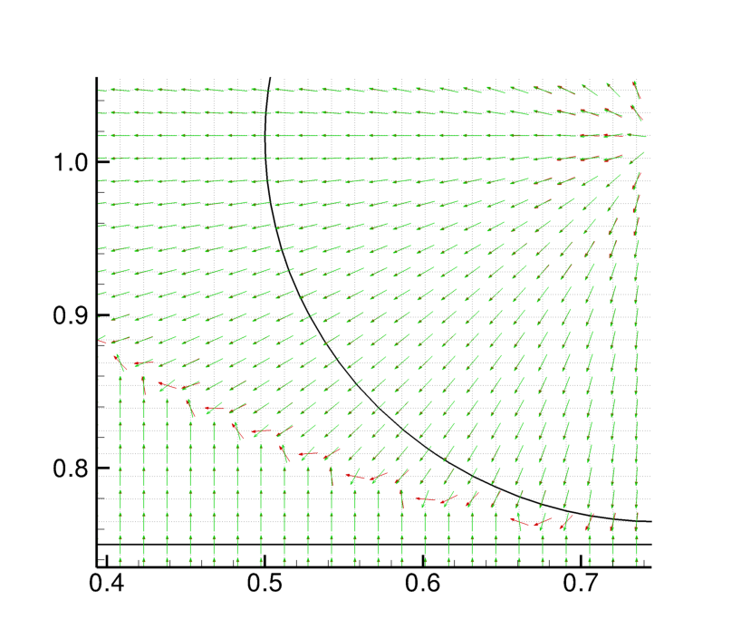
Figure 7: A comparison of the calculated normal vectors between the standard discretization in red and the improved method in green. The thick black lines depict the interface.

Figure 8 shows a comparison of the calculated curvatures. Note that the curvature is only calculated at grid points adjacent to the interfaces. At the grid points where it is not calculated, it is set to zero. The figure shows that the standard discretization leads to large errors in the calculated curvatures in the areas that are close to two interfaces. In particular note that the sign of the curvature becomes wrong. The analytic curvature for this case is $\kappa=-1/r=-4$, and the curvature spikes seen for the standard discretization is in the order of $|\kappa|\sim\frac{1}{\Delta x}\simeq 67.3$. These spikes will lead to large errors in the pressure jumps through Equation 17. The effect of these errors will become more clear in the next case.

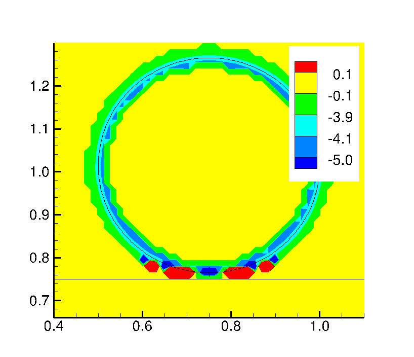
(a) Standard discretization

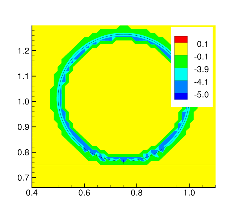
(b) Improved method with curve fitting

Figure 8: A comparison of curvature calculations between standard discretization and the improved method. The standard discretization leads to large errors in the curvatures in areas that are close to two interfaces.

6.2 Drop collision in shear flow

The second case considers drop collision in shear flow, see Figure 9. The drops both have a radius $r$, and they are initially placed at a distance $d=5r$ apart in a shear flow where the flow velocity changes linearly from $u_{s}=-U<0$ at the bottom wall to $u_{n}=U$ at the top wall. The computational domain is $12r\times 8r$, and the grid size is $241\times 161$. The size of the grid is chosen to be relatively coarse, such that the difference between the standard discretization of the curvature and the curve-fitting based discretization is properly revealed.

Figure 9: The drop in shear setup.

The purpose of this case is to study the behaviour of the level-set method, in particular the calculation of the curvatures, when the drops are in close proximity. It is therefore a natural simplification to only consider the case where the density difference and the viscosity difference of the phases are zero, i.e. there is no jump in density or viscosity across the interface.

The flow is governed by the Reynolds number and the Capillary number, which in the current case can be defined by

$$Re =\frac{\rho Ur}{4\mu},$$ (39)

$$Ca =\frac{\mu U}{4\sigma}.$$ (40)

In the following results the Reynolds and the Capillary numbers were set to

$$Re=10,\quad Ca=0.025.$$ (41)

The choice was made such that the drops would not be severely deformed in the shear flow. The radius of the drops was $r=0.5\ \mathrm{m}$, and the distance from the center line to the drop centers was $h=0.84r=0.42\ \mathrm{m}$.

Figure 10 shows a comparison of the interface evolution and the curvature between the standard discretization and the improved discretization. The top and bottom rows show the evolution for the standard discretization and the improved discretization, respectively. The kinks between the drops lead to curvature spikes with the standard discretization, whereas the improved discretization calculates the curvature along the kink in a much more reliable manner. The curvature spikes are seen to prevent coalescence. This is due to the effect they have on the pressure field.

Figure 10: A comparison between the standard discretization (top row) and the improved discretization (bottom row) of the interface evolution and the curvature $\kappa$ of drop collision in shear.

The errors in the curvature with the standard discretization lead to an erroneous pressure field between the drops that prevents coalescence, c.f. Equation 16. Figure 11 shows the pressure field at $t=2.75\ \mathrm{s}$. It can be seen that the pressure field for the standard discretization is distorted in the thin-film region. This distortion in the pressure leads to a flow in the film region which suppresses coalescence. The corresponding result for the improved method shows that the pressure is not distorted. It is high in the center of the thin-film region and lower at the edges. The pressure change induces a flow out of the region which is more as expected.

(a) Standard discretization

(b) Improved method

Figure 11: Comparison of the pressure field in the thin film between the droplets at $t=2.75\ \mathrm{s}$. The contour legends indicate the pressure in Pa .

7 Conclusions

This article has implemented improved discretization schemes for the normal vector and the curvature of the interface between two phases. The normal vector was discretized by the direction difference which is presented in [11]. The curvature was discretized with a scheme that is based on the geometry-aware discretization presented in [12]. The main advantage of the present discretization method for the curvature is that it is relatively straightforward to implement in to an existing code since it does not require a change of the existing framework.

The implementation of the curvature discretization have been described in detail. The improved schemes are compared with the standard discretization in two different cases. The first case is a direct comparison of the schemes for a case with no flow. The second case compares the evolution of two drops colliding in shear flow. Both tests demonstrate that the standard discretization of the normal vector and the curvature leads to erroneous behaviour at the kink locations. The second case shows that this behaviour prevents coalescence from occurring due to an erroneous pressure field. The curvature spikes at the kink regions are not observed with the improved discretization schemes, and coalescence is achieved for the second case.

References

- [1] D.Adalsteinsson and J. A.Sethian A fast level set method for propagating interfaces Journal of Computational Physics, vol.118, 269–277, 1995.
- [2] O.Desjardins, V.Moureau and H.Pitsch An accurate conservative level set/ghost fluid method for simulating turbulent atomization Journal of Computational Physics, vol.227, 8395–8416, 2008.
- [3] F. N.Fritsch and R. E.Carlson Monotone piecewise cubic interpolation SIAM Journal of Numerical Analysis, vol.17(2), 238–246, 1980.
- [4] S.Gottlieb, C. W.Shu and E.Tadmor Strong stability-preserving high-order time discretization methods SIAM Review, vol.43, 89–112, 2001.
- [5] E. B.Hansen Numerical Simulation of Droplet Dynamics in the Presence of an Electric Field Doctoral thesis, Norwegian University of Science and Technology, Department of Energy and Process Engineering, Trondheim, Nov. 2005 ISBN 82-471-7318-2.
- [6] M.Herrmann A balanced force refined level set grid method for two-phase flows on unstructured flow solver grids Journal of Computational Physics, vol.227, 2674–2706, 2008.
- [7] M.Kang, R. P.Fedkiw and X.-D.Liu A boundary condition capturing method for multiphase incompressible flow Journal of Scientific Computing, vol.15(3), 323–360, 2000.
- [8] S.Lang Algebra Graduate texts in mathematics. Springer, 2002.
- [9] X.-D.Liu, R. P.Fedkiw and M.Kang A boundary condition capturing method for poisson’s equation on irregular domains Journal of Computational Physics, vol.160, 151–178, 2000.
- [10] W. E.Lorensen and H. E.Cline Marching cubes: A high resolution 3D surface construction algorithm Computer Graphics, vol.21(4), 163–169, July 1987.
- [11] P.Macklin and J.Lowengrub Evolving interfaces via gradients of geometry-dependent interior poisson problems: Application to tumor growth Journal of Computational Physics, vol.203, 191–220, 2005.
- [12] P.Macklin and J.Lowengrub An improved geometry-aware curvature discretziation for level set methods: Application to tumor growth Journal of Computational Physics, vol.215, 392–401, 2006.
- [13] P.Macklin and J. S.Lowengrub A new ghost cell/level set method for moving boundary problems: Application to tumor growth Journal of Scientific Computing, vol.35, 266–299, 2008.
- [14] E.Marchandise, P.Geuzaine, N.Chevaugeon and J.-F.Remacle A stabilized finite element method using a discontinuous level set approach for the computation of bubble dynamics Journal of Computational Physics, vol.225, 949–974, 2007.
- [15] S.Osher and R. P.Fedkiw The Level-Set Method and Dynamic Implicit Surfaces Springer, 2003.
- [16] S.Osher and J. A.Sethian Fronts propagating with curvature dependent speed: Algorithms based on Hamilton-Jacobi formulations Journal of Computational Physics, vol.79, 12–49, 1988.
- [17] H.Prautzsh, W.Boehm and M.Paluszny Bézier and B-spline Techniques Springer, 2002.
- [18] D.Salac and W.Lu A local semi-implicit level-set method for interface motion Journal of Scientific Computing, vol.35, 330–349, 2008.
- [19] J. A.Sethian and P.Smereka Level set methods for fluid interfaces Annual Review of Fluid Mechanics, vol.35, 341–372, 2003.
- [20] M.Sussman, P.Smereka and S.Osher A level set approach for computing solutions to incompressible two-phase flow Journal of Computational Physics, vol.114, 146–159, 1994.
- [21] B.Waerden, E.Artin and E.Noether Algebra Number v. 1 in Algebra. Springer-Verlag, 2003.
- [22] Z.Wang and A. Y.Tong A sharp surface tension modeling method for two-phase incompressible interfacial flows International Journal for Numerical Methods in Fluids, vol.64, 709–732, 2010.
- [23] J.-J.Xu, Z.Li, J.Lowengrub and H.Zhau A level set method for interfacial flows with surfactants Journal of Computational Physics, vol.212(2), 590–616, March 2006.
- [24] H. K.Zhao, T.Chan, B.Merriman and S.Osher A variational level set approach to multiphase motion Journal of Computational Physics, vol.127, 179–195, 1996.