Determination of Three-dimensional Spin–orbit Angle
with Joint Analysis of Asteroseismology, Transit Lightcurve,
and the Rossiter–McLaughlin Effect: Cases of HAT-P-7 and Kepler-25

Abstract

We develop a detailed methodology of determining three-dimensionally the angle between the stellar spin and the planetary orbit axis vectors, $\psi$, for transiting planetary systems. The determination of $\psi$ requires the independent estimates of the inclination angles of the stellar spin axis and of the planetary orbital axis with respect to the line-of-sight, $i_{\star}$ and $i_{\rm orb}$, and the projection of the spin–orbit angle onto the plane of the sky, $\lambda$. These are mainly derived from asteroseismology, transit lightcurve and the Rossiter-McLaughlin effect, respectively. The detailed joint analysis of those three datasets enables an accurate and precise determination of the numerous parameters characterizing the planetary system, in addition to $\psi$.

We demonstrate the power of the joint analysis for the two specific systems, HAT-P-7 and Kepler-25. HAT-P-7b is the first exoplanet suspected to be a retrograde (or polar) planet because of the significant misalignment $\lambda\approx 180^{\circ}$. Our joint analysis indicates $i_{\star}\approx\timeform{30D}$ and $\psi\approx 120^{\circ}$, suggesting that the planetary orbit is closer to polar rather than retrograde. Kepler-25 is one of the few multi-transiting planetary systems with measured $\lambda$, and hosts two short-period transiting planets and one outer non-transiting planet. The projected spin–orbit angle of the larger transiting planet, Kepler-25c, has been measured to be $\lambda\approx 0^{\circ}$, implying that the system is well-aligned. With the help of the tight constraint from asteroseismology, however, we obtain $i_{\star}=\timeform{65D.4}^{+\timeform{10D.6}}_{-\timeform{6D.4}}$ and $\psi=\timeform{26D.9}^{+\timeform{7D.0}}_{-\timeform{9D.2}}$, and thus find that the system is actually mildly misaligned. This is the first detection of the spin–orbit misalignment for the multiple planetary system with a main-sequence host star, and points to mechanisms that tilt a stellar spin axis relative to its protoplanetary disk.

1 Introduction

The spin–orbit angle between the stellar spin and the planetary orbital axes, $\psi$, is supposed to be a unique observational probe of the origin and evolution of planetary systems. The existence of Jupiter-like planets with orbital periods less than a week strongly indicates that the inward migration of those planets is a basic ingredient of successful theories of planet formation and evolution. A fairly popular scenario of the migration is based on the planet–disk interaction, in which planets are supposed to be on circular orbits whose orbital axes are parallel to the stellar spin axis. On the other hand, scenarios such as planet–planet scattering or the Kozai mechanism predict a broad range of eccentric and oblique orbits. Thus the precise determination of $\psi$ and its statistical distribution put a tight constraint on the viable migration models (Queloz et al., 2000; Winn et al., 2005).

While the measurement of $\psi$ is not easy, its projection onto the plane of the sky, $\lambda$, has already been measured for more than 70 transiting planetary systems via the Rossiter–McLaughlin (RM) effect (Winn, 2011), and is now established as one of the most basic parameters that characterize transiting planetary systems.

The RM effect was originally proposed to determine the projected spin–orbit angle of eclipsing binary star systems (Rossiter, 1924; McLaughlin, 1924). Queloz et al. (2000) successfully applied the technique for the first discovered transiting exoplanetary system, HD 209458, and obtained $\lambda=\pm\timeform{3D.9}{+18^{\circ}\atop-21^{\circ}}$. In the quest for improving the precision and accuracy, Ohta et al. (2005) presented an analytic formula to describe the RM effect and studied in detail the error budget and possible degeneracy among different parameters. This allowed Winn et al. (2005) to revisit HD 209458 with updated photometric and spectroscopic data, and to obtain $\lambda=-\timeform{4^{D}.4}\pm\timeform{1D.4}$, improving the precision of the previous measurement by an order of magnitude.

In doing so, Winn et al. (2005) pointed out that the analytic approximation adopted by Ohta et al. (2005) leads to typically 10 percent error in the predicted velocity anomaly amplitude, while the estimated $\lambda$ is fairly reliable. This motivated Hirano et al. (2010) and Hirano et al. (2011) to take into account stellar rotation, macroturbulence, and thermal/pressure/instrumental broadenings in modeling the stellar absorption line profiles. Those authors derived an analytic formula for the velocity anomaly of the RM effect by maximizing the cross-correlation function between the in-transit spectrum and the stellar template spectrum. As a result, their analytic formulae reproduce mock simulations within $\sim 0.5$ percent, enabling the accurate and efficient multi-dimensional fit of parameters characterizing the star and planet(s) of an individual system.

More importantly, Winn et al. (2005) clearly demonstrated the potential of the RM effect to put strong quantitative constraints on the existing and/or future planetary formation scenarios. Indeed, when HD 209458 was the only known transiting planetary system, Ohta et al. (2005) discussed that “Although unlikely, we may even speculate that a future RM observation may discover an extrasolar planetary system in which the stellar spin and the planetary orbital axes are anti-parallel or orthogonal. Then it would have a great impact on the planetary formation scenario, …”. In reality, however, they were too conservative. Among the 70 transiting planetary systems observed with the RM effect, more than 30 systems exhibit significant misalignment with $|\lambda|>\timeform{22D.5}$ [ see, e.g., figure 7 of Xue et al. (2014) ]. This unexpected diversity of the spin–orbit angle is not yet properly understood by the existing theories, and remains an interesting challenge (see, Fabrycky & Tremaine, 2007; Nagasawa et al., 2008; Winn et al., 2010; Nagasawa & Ida, 2011; Hirano et al., 2012a, b; Lai, 2012; Albrecht et al., 2013; Masuda et al., 2013; Xue et al., 2014).

It should be noted, however, that $\lambda$ differs from the true spin–orbit angle $\psi$ due to the projection on the sky. In addition to $\lambda$, $\psi$ also depends on the orbital inclination $i_{\rm orb}$ and the obliquity of the stellar spin-axis $i_{\star}$:

$$\cos\psi=\cos i_{\star}\cos i_{\rm orb}+\sin i_{\star}\sin i_{\rm orb}\cos\lambda,$$ (1)

as illustrated in Figure 1.

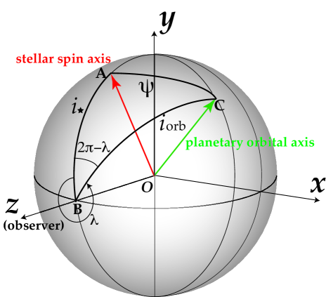
Figure 1: Schematic illustration of geometric configuration of star–planet systems. We choose a coordinate system centered on the star, where the $XY$-plane is in the plane of the sky and $+Z$-axis points towards the observer. The $+Y$-axis is chosen along the sky-projected stellar spin and the $X$-axis is perpendicular to both $Y$- and $Z$-axes, forming a right-handed triad. Red and green arrows indicate on a unit sphere, the angular momentum vectors of the stellar spin and the planetary orbital motion, respectively. The stellar and orbital inclinations, $i_{\star}$ and $i_{\rm orb}$, are measured from the $+Z$-axis and in the range of $[\,0^{\circ},180^{\circ}]$. The planetary orbital axis projected onto the sky plane is specified by the projected spin–orbit angle, $\lambda$, which is measured from the $+Y$-axis and in the range of $[0^{\circ},360^{\circ}]$. Note that $\lambda$ is measured in the direction specified by the arrow. The angle AOC between the stellar spin and the planetary orbit axis vectors, $\psi$, is derived from the law of cosines for the spherical triangles ABC, as given by Equation (1).

The main purpose of this paper is to establish a methodology to determine $\psi$, instead of $\lambda$, through the joint analysis of asteroseismology, transit lightcurve, and the RM effect, and to present specific results for a couple of interesting transiting planetary systems, HAT-P-7 (KIC 10666592) and Kepler-25 (KIC 4349452).

In the case of transiting planetary systems, $i_{\rm orb}$ can be estimated from the transit lightcurve, and in any case is close to $90^{\circ}$. Given the projected angle $\lambda$ measured from the RM effect, the major uncertainty for $\psi$ comes from the unknown stellar inclination $i_{\star}$.

There are two major and complementary approaches to estimate $i_{\star}$, and hence $\psi$. One is to determine the line-of-sight rotational velocity of the star, $v\sin i_{\star}$, either from the width of absorption lines or from the RM effect. The observed $v\sin i_{\star}$ is then compared with an independent estimate of the equatorial velocity of the star, $v$, to yield $i_{\star}$. Schlaufman (2010) used an empirical relation for Sun-like stars to evaluate $v$ from their masses and ages. Alternatively, one can determine the stellar spin period photometrically from periodic variations in the lightcurve due to the stellar activity, and then estimate $v$ assuming the stellar radius (e.g., Hirano et al., 2012a).

The other is asteroseismology (Unno et al., 1989; Aerts et al., 2010) for which the key principles are described in detail later, but briefly summarised below. Thanks to space-borne instruments such as MOST (Walker et al., 2003), CoRoT (Baglin et al., 2006a, b) and Kepler (Borucki et al., 2010), asteroseismology now opens a good opportunity to unveil the internal structure of many stars with high precision. This is made possible through the detection of oscillation modes propagating throughout the stars with unprecedented precision, because of extraordinary low noise level and uninterrupted extremely long-term data monitoring with short sampling cadences, both of which are never available from the ground-based observations (e.g. Appourchaux et al., 2008; Metcalfe et al., 2012; Gizon et al., 2013). More details about the recent development in asteroseismology may be found in recent conference proceedings such as Shibahashi et al. (2012), Shibahashi & Lynas-Gray (2013), and Guzik et al. (2014). When coupled with non-seismic observables, the asteroseismic observational information promises accurate inference of fundamental properties of host stars (e.g. Bazot et al., 2005; Carter et al., 2012).

The stellar rotation affects the frequency spectrum of stellar oscillation modes. It induces a multiplet fine structure, whose frequency separation is dependent on the internal rotation profile of the star as well as the stellar structure, for each mode. More importantly, the apparent profiles of the rotationally induced frequency multiplets are very sensitive to the inclination angle of the stellar rotation axis with respect to the line-of-sight, $i_{\star}$. In turn, one can infer $i_{\star}$ quite well from asteroseismology.

One might wonder how commonly stellar oscillations that enable asteroseismology can be detected among the host stars of exoplanet systems. Remember that transiting planet hunting preferentially select stars with small radii (i.e. low-mass stars in the main sequence) in order to increase the relative transit depth in the photometric lightcurve. Moreover, such low-mass stars are suitable for the radial velocity follow-up not only because they are more affected by orbital motion of planets but also because they have sharp and narrow absorption lines due to their slow spin rotation velocity. Such low-mass, cool stars have a thick convective envelope (as in the case of the Sun) that sustains pulsations. Turbulent motion with speeds close to that of sound near the stellar surface stochastically generates acoustic waves, which propagate inside the star until they are damped. The oscillations with frequencies close to those of eigenmodes of the star are eventually sustained as many acoustic modes. Therefore cool (i.e. $\lessapprox 7000$ K) host stars for exoplanets should commonly exhibit solar-like oscillations, and thus consitute good targets for asteroseismology.

In this paper, we focus on two specific exoplanetary systems, HAT-P-7 and Kepler-25; HAT-P-7 is the first example of a system hosting a retrograde or a polar-orbit planet, while Kepler-25 is a multi-transiting system with three planets, making them two interesting examples. We show that joint analyses of asteroseismology, transit lightcurve, and the RM effect provide stringent orbital parameter estimates.

This paper is organised as follows. Section 2 summarizes the previous RM measurements and radial velocity (RV) data of the two systems. Section 3 presents a detailed description of the basic principle of asteroseismology, followed by our main results of asteroseismology for the two stars in Sections 4 and 5. Sections 6 and 7 analyze the Kepler transit lightcurves and the RV anomaly of the RM effect, using the asteroseismology results as a prior, and show how the joint analysis improves the estimates of the system parameters. Section 8 is devoted to further discussion, and Section 9 summarises the present paper.

2 Previous Spin–Orbit Measurements

2.1 HAT-P-7

The HAT-P-7 system comprises a bright (V=10.5) F6 star and a hot Jupiter transiting the host star with a 2.2-d period (Pál et al., 2008, hereafter P08). In addition to the significant spin–orbit misalignment first revealed by the Subaru spectroscopy (Narita et al., 2009; Winn et al., 2009), the fact that the system is in the Kepler field makes it very attractive as an asteroseismology target.

Interestingly, there have been three independent measurements of the RM effect for the HAT-P-7 system, which all indicate the significant spin–orbit misalignment, but do not agree quantitatively. Winn et al. (2009) (hereafter W09) performed the joint analysis of the spectroscopic and photometric transit of HAT-P-7b to obtain $\lambda=\timeform{182D.5}\pm\timeform{9D.4}$. For RVs, they analyzed 17 spectra observed with the High Resolution Spectrograph (HIRES) on the Keck I telescope as well as 69 spectra observed with the High Dispersion Spectrograph (HDS) on the Subaru telescope. Eight of the HIRES spectra were from P08 and taken in 2007, while the other nine were obtained in 2009. Among 69 HDS spectra, 40 were obtained on 2009 July 1 that spanned a transit.

On the other hand, Narita et al. (2009) (hereafter N09) determined $\lambda=\timeform{227D.4}{+\timeform{10D.5}\atop-\timeform{16D.3}}$ (equivalently $\lambda=-\timeform{132D.6}{+\timeform{10D.5}\atop-\timeform{16D.3}}$) based on the eight HIRES RVs from P08 and 40 HDS spectra spanning the transit on 2008 May 30. Although they fixed the transit parameters in the analysis of the RM effect, the systematics from the uncertainties of these parameters do not seem to explain the mild discrepancy with the W09 result, according to their discussion (see cases 1 to 4 in section 4 of N09).

Later on, Albrecht et al. (2012) (hereafter A12) reported another measurement of the RM effect, resulting in $\lambda=\timeform{155D}\pm 14^{\circ}$. They analyzed 49 HIRES spectra spanning a transit on the night 2010 July 23/24 with the priors on transit parameters and ephemeris from the Kepler lightcurves.

In this paper, we use the same RV data published in each of the three papers. Since the origin of the possible discrepancy in $\lambda$ is not clear, we analyze each data set separately instead of combining the three.

2.2 Kepler-25

The Kepler-25 system is one of the few multi-transiting planetary systems with constrained $\lambda$. It consists of a relatively bright ($K_{\rm p}=10.7$) host star, two short-period Neptune-sized planets confirmed with Transit Timing Variations (TTVs) (Steffen et al., 2012), and one outer non-transiting planet detected in long-term RV trend (Marcy et al., 2014). Albrecht et al. (2013) (hereafter A13) measured $\lambda=7^{\circ}\pm 8^{\circ}$ for the larger transiting planet Kepler-25c based on the HIRES spectra observed for two nights (2011 July 18/19 and 2012 May 31/June 1). Since the signal-to-noise ratio of the RV anomaly was small due to the relatively small radius of Kepler-25c, they also analyzed the time-dependent distortion of the spectral lines directly [known as the “Doppler shadow” method; see Collier Cameron et al. (2010)] and obtained a consistent result, $\lambda=-\timeform{0D.5}\pm\timeform{5D.7}$.

In this paper, we analyze the RVs around the above two transits from A13 alone because our focus is the determination of $\psi$.

3 Asteroseismology

3.1 Setting Up the Problem

Due to its sensitivity to the stellar internal structure, asteroseismology can achieve high-precision determinations of stellar fundamental parameters (Lebreton & Montalbán, 2009) (e.g., uncertainties of a few percent level for their mass and radius). The stellar modelling using seismic observables mostly relies on the stellar pulsation frequencies, usually extracted from the analysis of the power spectrum of the stellar lightcurve.

For a spherically symmetric star, each eigenmode is characterised by three quantum numbers; the angular degree $l$, the azimuthal order $m$ ($-l\leq m\leq+l$), and the radial order $n$. The degree $l$ corresponds to the number of nodal surface lines, while the azimuthal order $m$ specifies the surface pattern of the eigenfunction, with $|m|$ being the number of longitude lines among the $l$ nodal surface lines. The radial order $n$ corresponds to the number of nodal surfaces along the radius. For a non-rotating star, both the radial eigenfunction and the frequency of each mode are independent of $m$ and show the $(2l+1)$-fold degeneracy. The eigenfrequency $\nu$ depends on $l$ and $n$ alone. Frequencies of high order, acoustic (or p-) modes of the same low degree $(n\gg l\sim 1)$ are almost equally spaced and separated on average by a frequency spacing $\Delta\nu$:

$$\nu(n,l)=\Delta\nu\left(n+{{l}\over{2}}+\alpha\right)+\varepsilon_{n,l},$$ (2)

where $\alpha$ is a constant of order unity, and $\varepsilon_{n,l}$ is a small correction. The spacing is related to the sound velocity inside the star by

$$\Delta\nu=\left(2\int_{0}^{R_{\star}}{{1}\over{c(r)}}\,dr\right)^{-1}$$ (3)

and is sensitive to the mean stellar density $\rho_{\star}$. Therefore, knowing the solar density $\rho_{\odot}=(1.4060\pm 0.0005)\times 10^{3}$ kg m^-3 and its frequency spacing $\Delta\nu_{\odot}=135.20\pm 0.25$ $\mu$Hz, one can estimate the mean stellar density from the scaling:

$$\rho_{\star,\mathrm{s}}=\rho_{\odot}(\Delta\nu/\Delta\nu_{\odot})^{2}.$$ (4)

The stellar rotation lifts the degeneracy among non-radial modes ($l\neq 0$), revealing a fine structure of modes identified by their azimuthal order $m$. In the case of solar-like oscillations, acoustic modes are excited stochastically by turbulent convection. This mechanism is expected to generate almost the same amplitudes in the rotationally split modes with the same $l$ and $n$. If this is the case, in disk-integrated photometry as achieved by Kepler, the height of the azimuthal modes in the power spectrum is sensitive to the stellar inclination angle $i_{\star}$ due to a geometrical projection effect [see Gizon & Solanki (2003) for more details] and has been widely used to evaluate $i_{\star}$ (e.g. Benomar et al., 2009b; Appourchaux et al., 2012). In turn, it enables us to measure $\psi$ of exoplanets (Chaplin et al., 2013; Van Eylen et al., 2014), and indeed revealed a significant spin–orbit misalignment for a red-giant host star system, Kepler-56 (Huber et al., 2013b). This dependence of visibility in the power spectrum is expressed in terms of

$$\mathcal{E}(l,m,i_{\star})=\frac{(l-|m|)!}{(l+|m|)!}\left[P^{|m|}_{l}(\cos i_{\star})\right]^{2},$$ (5)

where $P^{|m|}_{l}$ is the associated Legendre function and the integral of $\mathcal{E}(l,m,i_{\star})$ over $\cos i_{\star}$ is normalised by $(2l+1)^{-1}$.

Solar-like oscillators such as Kepler-25 and HAT-P-7 are typically slow rotators for which the centrifugal force can be neglected. In addition, there is no evidence of a strong magnetic field and we can safely neglect it (Reese et al., 2006; Ballot, 2010). If the internal rotation of the star is independent of the latitude and the longitude, the split frequencies are simply written as

$$\nu(n,l,m)=\nu(n,l)+m\,\delta\nu_{\rm s}(n,l),$$ (6)

where $\delta\nu_{\rm s}(n,l)$ is the rotational splitting [e.g. Appourchaux et al. (2008); Benomar et al. (2009a); Chaplin et al. (2013)].

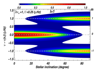
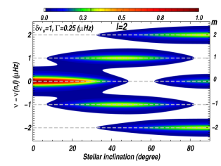
Figure 2: The figures illustrate the dependence between stellar inclination and rotation. The relative power of azimuthal components $m$ for $l=1$ and $l=2$ in the ideal case ($\delta\nu_{s}\gg\Gamma$) is indicated by the color scale and is calculated using Equation 7. Horizontal dash lines indicate frequencies of the multiplets $m$. Each inclination is characterised by a unique $l=1$ and $l=2$ mode structure. This property is used to infer the stellar inclination. Zero degree corresponds to a star seen from a pole, 90 degree to a star seen from the equator.

Table 1: Non-seismic observables of HAT-P-7 and Kepler-25. All but $v\sin i_{\star}$ are used for stellar modelling.

Star	$L/L_{\odot}$	$\log g$ (cgs)	[Fe/H]	$T_{\rm eff}$ (K)	$v\sin i_{\star}$ (km s-1)	Source
HAT-P-7	$4.9\pm 1.1$	$4.070\pm 0.06$	$0.26\pm 0.08$	$6350\pm 80$	$3.8\pm 0.5$	Pál et al. (2008)
Kepler-25	N/A	$4.278\pm 0.03$	$-0.04\pm 0.10$	$6270\pm 79$	$9.5\pm 0.5$	Marcy et al. (2014)

Table 2: Detected pulsation frequencies of HAT-P-7 and Kepler-25. The radial order $n$ is determined by the best models matching observables.

	HAT-P-7			Kepler-25
$l$	$n$	$\nu_{n,l,m=0}$	$\sigma$	$n$	$\nu_{n,l,m=0}$	$\sigma$
		($\mu$Hz)	($\mu$Hz)		($\mu$Hz)	($\mu$Hz)
0	11	715.50	0.30	16	1691.79	0.52
0	12	771.57	0.51	17	1788.58	0.23
0	13	828.34	0.30	18	1884.39	0.36
0	14	885.91	0.26	19	1981.33	0.18
0	15	944.88	0.25	20	2080.08	0.32
0	16	1004.77	0.22	21	2178.68	0.43
0	17	1064.83	0.20	22	2277.00	0.32
0	18	1123.17	0.23	23	2375.48	0.67
0	19	1181.90	0.23	24	2472.91	0.59
0	20	1240.53	0.27	25	2570.03	1.43
0	21	1300.53	0.35
0	22	1360.78	0.43
0	23	1421.55	0.94
0	24	1482.03	0.75
0	25	1542.96	1.21
1	11	740.79	0.22	16	1736.27	0.79
1	12	796.71	0.35	17	1832.49	0.20
1	13	854.00	0.23	18	1929.17	0.28
1	14	911.89	0.20	19	2026.97	0.28
1	15	971.85	0.16	20	2125.46	0.32
1	16	1031.54	0.15	21	2224.32	0.51
1	17	1091.15	0.15	22	2323.04	0.32
1	18	1149.92	0.17	23	2421.68	0.53
1	19	1208.36	0.17	24	2521.29	0.63
1	20	1267.82	0.23	25	2621.12	1.12
1	21	1327.41	0.27
1	22	1388.49	0.36
1	23	1448.96	0.46
1	24	1509.40	0.54
1	25	1569.30	0.92
2	10	710.81	0.63	15	1683.26	3.88
2	11	767.31	0.62	16	1779.57	2.17
2	12	824.46	0.53	17	1875.12	1.39
2	13	882.27	0.54	18	1972.55	0.67
2	14	940.46	0.34	19	2071.55	0.77
2	15	1000.17	0.49	20	2170.64	0.88
2	16	1059.82	0.35	21	2269.90	1.14
2	17	1118.74	0.31	22	2368.62	1.16
2	18	1177.89	0.39	23	2467.03	1.38
2	19	1236.33	0.42	24	2565.48	2.79
2	20	1296.40	0.50
2	21	1356.39	0.50
2	22	1417.09	0.97
2	23	1478.41	0.97
2	24	1539.79	1.50

It should be noted that because of the modes stochastic nature, each solar-like mode has a Lorentzian profile in the power spectrum (Harvey, 1985). Thus, the stellar oscillations can be expressed as a sum of Lorentzian over $n$, $l$ and $m$,

$$P(\nu)=\sum_{n,l}\sum_{m=-l}^{l}\frac{\mathcal{E}(l,m,i_{\star})H(n,l)}{1+4(\nu-\nu(n,l,m))^{2}/\Gamma^{2}(n,l,m)}.$$ (7)

Each mode is therefore not only characterised by its frequency $\nu(l,n,m)$, but also by a height $H(n,l,m)=\mathcal{E}(l,m,i_{\star})H(n,l)$ and a full width at half maximum $\Gamma(n,l,m)$ (hereafter called width). Here, $H(n,l)$ is the intrinsic height for the mode of $n$ and $l$. The heights and the widths of the modes retain information on, for example, the modes excitation mechanism and on non-adiabatic processes.

In order to show the sensitivity of the asteroseismology analysis to $i_{\star}$, we plot $P(\nu)$ in Figure 2 as a function of $i_{\star}$ and $\nu-\nu(n,l)$. The left and right panels correspond to $l=1$ and $l=2$ modes, respectively. The plot is color-coded according to the amplitude of $P(\nu)$ and for a given $n$ (i.e, a sum of the $(2l+1)$ Lorentzian profiles). Figure 2 is presented simply for illustrative purpose, and is computed from equations (5) and (7), assuming $\delta\nu_{\rm s}=1\,\mu$Hz and $\Gamma=0.25\mu$Hz. The condition $\delta\nu_{\rm s}\gg\Gamma$ breaks the degeneracy among the rotationally split $m$ components. As demonstrated in this figure, in the case of $i_{\star}\simeq 0^{\circ}$, that is, when we see the star from the pole, only the $m=0$ component is visible as a singlet for both of $l=1$ and $l=2$ modes. On the other hand, in the case of $i_{\star}\simeq 90^{\circ}$, the rotational splitting appears as a doublet in the case of $l=1$ and as a triplet in the case of $l=2$. Thus for a given value of $i_{\star}$, the power is the result of a unique configuration of height for the $m$ components, which enables us to infer the value of $i_{\star}$ from the $l=1$ and $l=2$ mode profiles. Note, however, that because Equation (5) depends on $|m|$ , solutions in the four quadrants of the trigonometric circle are degenerate and one cannot distinguish between $i_{\star}$ and $(180^{\circ}-i_{\star})$.

3.2 Data processing and modeling

The Kepler Space Telescope collected time series lightcurves of about 160,000 stars over the 115 square degrees field-of-view from its 372.5-d, heliocentric Earth-trailing orbit over its four-year lifetime for 2009 – 2013. Its major purpose was to find extra-solar planets by detecting a small amount drop of the visual brightness of their parent stars, caused by the transits of the planets in front of the stars. So the photometric asteroseismology and planet studies are synergistic. Four times per orbit the satellite was scheduled to perform a roll to keep its solar panels facing the Sun, so the data were divided into ‘Quarters’ (1/4 of its 372.5-d heliocentric orbit), denoted as Q$n$.

For HAT-P-7, we use Q0 to Q16 (1437 days in total) of Kepler data taken every 1-min (‘Short Cadence’ data; SC), while for Kepler-25, we used Q5 to Q16 (1114 days) SC data. After removing the transits from the lightcurve with a median high-pass filter of an adequate frequency width, we compute the power spectrum of each star following the method described in García et al. (2011b). The high-pass filter is efficient to remove the signal of the transit in the power spectrum without altering the stellar pulsation characteristics, since the orbital periods of the detected planets around HAT-P-7 and Kepler-25 are of the order of days, while stellar pulsation periods are in the minute range. To extract the mode parameters, we perform a Lorentzian profile fit to each mode that exhibits significant power. We use a Markov Chain Monte Carlo (MCMC) method and a similar method to Benomar et al. (2009a) but with a smoothness condition on the frequencies. (see Benomar et al., 2013, 2014).

The prior on the rotational splitting $\delta\nu_{\rm s}$ is uniform between 0 and 8 $\mu$Hz. The prior on $i_{\star}$ is chosen to be uniform in $\cos i_{\star}$ for $0<\cos i_{\star}<1$, and is equivalent to the random uniform distribution of $i_{\star}$. Because of the symmetries in Equation (5), we only consider solutions of $0^{\circ}\leq i_{\star}\leq 90^{\circ}$ in what follows.

Figures 3 and 4 show the resulting power spectra and their best-fit models for HAT-P-7 and Kepler-25, respectively. The identified pulsation modes and the derived pulsation frequencies of the central component of multiplets are listed in Table 2.

Figure 3: HAT-P-7. Power spectrum over three radial orders for modes with highest signal-to-noise ratio. The spectrum is shown after a boxcar smooth over $0.08$ $\mu$Hz (grey) and $0.24$ $\mu$Hz (black). The best fit is the solid red line. The inset shows all the extracted modes.

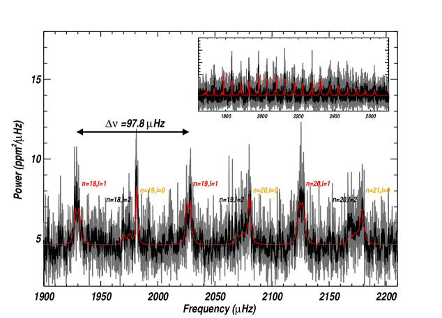
Figure 4: Kepler-25. Power spectrum over three radial orders for modes with highest signal-to-noise ratio. The spectrum is shown after a boxcar smooth over $0.21$ $\mu$Hz (grey) and $0.83$ $\mu$Hz (black). The best fit is the solid red line. The inset shows all the extracted modes.

Stellar models that simultaneously match non-seismic observables (cf. Table 1) and seismic observables (frequencies in Table 2) are found using the ‘astero’ module of the Modules for Experiments in Stellar Astrophysics (MESA) evolutionary code (Paxton et al., 2011, 2013). Stellar models are calculated assuming a fixed mixing length parameter $\alpha_{\rm MLT}=2.0$ and an initial hydrogen abundance $X=0.7$. The opacities are calculated using the MESA standard equation of state from the opacity table in Asplund et al. (2009). These are applicable for stars with effective temperature $10^{3}\,\rm K<T_{\rm eff}<10^{4.1}\,\rm K$. Nuclear reactions are set to include standard hydrogen and helium burning; the pp-chain and the CNO cycle in addition to the triple alpha reaction.

It is known that semiconvective zones are present in stars of $\sim 1.5\,M_{\odot}$. Since a small convective core in such stars expands due to the growing importance of the CNO cycle, the opacity is larger at the outer side of the convective boundary than at its inner side. We adopt the M. Schwarzschild treatment to define the boundary between the convective and radiative zones in such a case. With expected mass larger than 1.2 $M_{\odot}$, HAT-P-7 and Kepler-25 may have a convective core. Then, the nature of the transition (e.g. sharp or smooth) between convective and radiative regions may have a significant impact on the seismic frequencies (e.g. Monteiro et al., 1994). Thus, to describe a possible extension of the convective zone inside the radiative zone, we have included an overshoot. Diffusion was not implemented. Mass $M_{\star}$, metallicity [Fe/H], helium abundance $Y$, the coefficient for overshooting $\alpha_{\rm ov}$, and age are treated as free parameters.

Eigenfrequencies are calculated assuming adiabaticity and using ADIPLS (Christensen-Dalsgaard, 2008). We apply surface effect corrections to the frequencies, following the method of Kjeldsen et al. (2008). The search for the best model involves a simplex minimisation approach (Nelder & Mead, 1965) using the $\chi^{2}$ criteria. Uncertainties are then estimated by evaluating the $\chi^{2}$ for solutions surrounding the best model and by weighing the model parameters with Likelihood $\propto\exp(-\chi^{2}/2)$.

3.3 Mode Degree Identification

Prior to modelling a star, it is important to identify the degree $l$ from the power spectrum. In solar-like cool stars (K, G type) the identification is often obvious and relies on the échelle diagram (Grec et al., 1983). An échelle diagram is built by dividing the power spectrum into frequency bins of interval $\Delta$, that are stacked in order to form an image in which the power is color-coded. In this image, the Y-axis represents the central frequency of each bin, while the X-axis corresponds to the frequency modulo $\Delta$. Note that the central frequency of the bins is a discrete quantity and one could use instead an integer for the Y-axis. Figures 5 and 6 are the corresponding échelle diagram for HAT-P-7 and Kepler-25 stacked with $\Delta=59.9\,\mu$Hz and $\Delta=97.8\,\mu$Hz, respectively. If we choose $\Delta=\Delta\nu$, the excess power due to the modes of the same degree $l$ should show up along an almost straight vertical line. This is because p-modes of the same degree are almost regularly spaced in frequency, as implied by Equation (2).

Equation (2) shows that $\nu({n,l})=\nu({n-1,l+2})$ as long as $\varepsilon_{n,l}$ is small. Thus the eigenmodes of ($n$, $l=0$) and ($n-1$, $l=2$) have approximately the same frequencies. The same is true for ($n$, $l=1$) and ($n-1$, $l=3$). On the other hand, the pulsation amplitude of the surface, and consequently the integrated luminosity variation, are smaller for larger $l$ modes. Thus, the detected photometric amplitudes of the pulsation are usually dominated by $l=0$ and $l=1$, and $l\geq 3$ are often buried in the noise.

This is why the careful visual inspection of the relative height and frequency of the power spectra enable us to identify the corresponding modes. This approach works for Kepler-25, but not for HAT-P-7 in reality. The power spectrum of HAT-P-7 exhibits significant mixture of $l=0$ and $l=2$ modes, and it is hard to disentangle them by visual inspection. In such a case that the modes of the same $l$ are almost regularly spaced in frequency, there exist two possibilities: either (S1) the fit misidentifies the modes, or (S2) the fit correctly identifies the mode. As for the former, all modes of degrees $l=0$ and $l=2$ would be misidentified as $l=1$ modes (and vice-versa). This problem of mode identification is recurrent in F stars and was first encountered in a star observed by CoRoT, HD 49933 (Appourchaux et al., 2008).

The most likely solution among the two competitive solutions (S1) and (S2) described above may be judged by the Bayes factor between S1 and S2 [see Benomar et al. (2009a, b); Appourchaux et al. (2012) for more details]. Using our MCMC samples, we evaluated the Bayes factor at $10^{6}:1$ in favour of modes with frequencies listed in Table 2. According to Jeffreys (1961) , the Bayes factor $>100$ is “Decisive”, and thus one can safely assume that the mode identification is correct. We also note that use of the empirical approach detailed in White et al. (2012) reproduces the same degree identification.

Furthermore, there is not clear evidence for $l=3$ in the échelle diagram. To verify this quantitatively, we attempted to detect modes of degree $l=3$ by comparing the Bayes factor between a model $M_{l\leq 3}$, that includes those modes, with a model $M_{l\leq 2}$ that does not. We obtained a factor $\simeq 2:1$ and $\simeq 2.5:1$ for HAT-P-7 and Kepler-25 respectively, in favour of $M_{l\leq 2}$, which is the simplest model. Thus modes of degree $l=3$ are not conclusively detected.

Table 3: Stellar model characteristics for HAT-P-7 and Kepler-25 derived with MESA. $\rho_{\star,\rm m}$ is the density derived from modelling. $\rho_{\star,\rm s}$ is the density derived by rescaling the Sun density using the average frequency separation $\Delta\nu$.

parameter	HAT-P-7	Kepler-25
$M_{\star}$ $(M_{\odot})$	$1.59\pm 0.03$	$1.26\pm 0.03$
$R_{\star}$ $(R_{\odot})$	$2.02\pm 0.01$	$1.34\pm 0.01$
$[{\rm Fe/H}]$	$0.32\pm 0.04$	$0.11\pm 0.03$
$T_{\rm eff}$ (K)	$6310\pm 15$	$6354\pm 27$
Age (Myrs)	$1770\pm 100$	$2750\pm 300$
$\alpha_{\rm ov}$	$0.000{{+0.002}\atop{-0.000}}$	$0.007\pm 0.003$
$L/L_{\odot}$	$5.84\pm 0.05$	$2.64\pm 0.07$
$\log g$ (cgs)	$4.029\pm 0.002$	$4.285\pm 0.003$
$\rho_{\star,\rm m}$ (103 kg m-3)	$0.2708\pm 0.0035$	$0.7367\pm 0.0137$
$\rho_{\star,\rm s}$ (103 kg m-3)	$0.2696\pm 0.0011$	$0.7356\pm 0.0030$
reduced $\chi^{2}$	$1.73$	$1.03$

4 Asteroseismology of HAT-P-7

The power spectrum of HAT-P-7 (Figure 3) shows a broad range of modes, spanning over 15 different radial orders with a high signal-to-noise ratio (Table 2), enabling us to infer modes properties with an unprecedented precision for an F-star. Our asteroseismic analysis detected a total of 45 modes of degree $l=0$, $1$ and $2$, for which the frequencies are listed in Table 2.

4.1 Fundamental Properties

The échelle diagram of HAT-P-7 (Figure 5) shows clear departures from a straight line, which is mostly the signature of the transition between the outer convective zone and the radiative zone. This is because discontinuities within the structure translate into steep gradients in the acoustic structure of a star, which induce frequency modulations of periods related to the acoustic depth of the discontinuities (e.g. Vorontsov, 1988; Monteiro et al., 1994; Roxburgh & Vorontsov, 2003). In modelling HAT-P-7, it is therefore important to find models that match not only the average frequency separation $\Delta\nu$ (which is sensitive only to the mean density) but also all individual frequencies accurately.

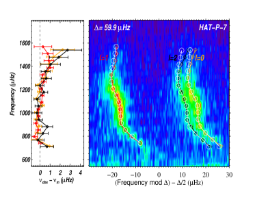
Figure 5: Left panel. Difference between observed frequencies $\nu_{\rm obs}$ of HAT-P-7 and best model frequencies $\nu_{\rm m}$. $l=0,1,2$ are shown as orange, red and black diamonds respectively. Right panel. Échelle diagram showing the observed power spectrum (background), the observed frequencies (diamonds) and the frequencies from the best model (white circles).

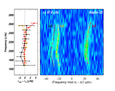
Figure 6: Left panel. Difference between observed frequencies $\nu_{\rm obs}$ of Kepler-25 and best model frequencies $\nu_{\rm m}$. $l=0,1,2$ are shown as orange, red and black diamonds respectively. Right panel. Échelle diagram showing the observed power spectrum (background), the observed frequencies (diamonds) and the frequencies from the best model (white circles).

Following the method described in Section 3.2, we found that the best model implies $M_{\star}=1.59\pm 0.03\,M_{\odot}$ (cf. Table 3 for main characteristics of the model), which is slightly greater than what was reported in earlier seismic studies; Christensen-Dalsgaard et al. (2010) used Q0 and Q1 Kepler data ($\approx 60$ days long) and reported $M_{\star}=1.520\pm 0.036\,M_{\odot}$. They fitted individual frequencies corrected from the surface effects (Kjeldsen et al., 2008) and they used the ASTEC evolutionary code with a method and physics similar to what we adopted in the present paper. Oshagh et al. (2013) carried out an analysis of HAT-P-7 using Kepler Q0 to Q2 (144 days long). Their approach slightly differs from ours as they did a non-adiabatic frequency calculation. They reported $M_{\star}=1.415\pm 0.020\,M_{\odot}$. Furthermore Van Eylen et al. (2012) used Kepler data from Q0 to Q11 and reported $M_{\star}=1.361\pm 0.021\,M_{\odot}$. While our model values are consistent with those quoted in Christensen-Dalsgaard et al. (2010) within $2\sigma$, the other estimates are significantly different. Thus we discuss the issue below.

First of all, Christensen-Dalsgaard et al. (2010) and our study result in consistent mean stellar densities at $1\sigma$. In contrast, Oshagh et al. (2013) obtain $\rho_{\star,\rm m}=(0.2778\pm 0.0059)\times 10^{3}$ kg m^-3 and Van Eylen et al. (2012) $\rho_{\star,\rm m}=(0.2781\pm 0.0017)\times 10^{3}$ kg m^-3, which are consistent within $1\sigma$. While the differences between Oshagh et al. (2013) and the present study may be due to the non-adiabatic treatment of model frequencies and to the data quality as well, this cannot explain the low mass found by Van Eylen et al. (2012). Nevertheless, although the model in figure 2 of Van Eylen et al. (2012) has a small value of $\chi^{2}$, it does not seem to reproduce accurately their individual frequencies. Moreover their method of measuring the frequencies differs from ours (frequencies are measured by taking the frequency at maximum height of a smooth spectrum) and they reported larger uncertainties than what we obtain here.

In order to see if the difference in methodology could explain the apparent discrepancies, we looked for the best model (minimum $\chi^{2}$) assuming $M_{\star}=1.36\,M_{\odot}$, to be coherent with Van Eylen et al. (2012). The best model has a $\chi^{2}=24.6$, approximately 14 times higher than the best model shown in Table 3 and does not reproduce accurately the individual oscillation frequencies. The mean stellar density $\rho_{\star,\rm m}=(0.2562\pm 0.0002)\times 10^{3}$ kg m^-3 is also significantly different. Thus we conclude that mass of $\approx 1.36\,M_{\odot}$ is less favored than $\approx 1.59\,M_{\odot}$, from our seismic observables.

The best-fit model of the present study implies that the HAT-P-7 has a convective core that extends up to 6.9% of the stellar radius, while the outer convective zone represents approximately 13.1% of the stellar radius. The central hydrogen abundance $X_{\rm c}=0.214$, which corresponds to 32% of its initial core hydrogen, indicates that the star is at a late stage in its main sequence. Finally we note that the best model of HAT-P-7 has no need of surface effect correction.

4.2 Rotation and Inclination

Figure 7 shows the joint probability density function (PDF) of $\delta\nu_{\rm s}$ and $i_{\star}$, $p(i_{\star},\delta\nu_{\rm s})$, for HAT-P-7 as well as their marginalised posterior PDF, $p(\delta\nu_{\rm s})$ and $p(i_{\star})$. As clearly illustrated, $i_{\star}$ of HAT-P-7 is not tightly constrained. The most probable value is $i_{\star}=\timeform{27D.3}{+\timeform{34D.9}\atop{-\timeform{17D.5}}}$ with a 68% confidence interval. This suggests that the star is more likely seen by its pole than by its equator, albeit with large uncertainty. To understand why $i_{\star}$ is not well determined, we show in Figure 8 the power $P(\nu)$ corresponding to the modes of degree $l=1$ and $l=2$ as we did in Figure 2, but we set the rotational splitting equal to the observed median splitting ($\delta\nu_{\rm s}=0.70\,\mu$Hz). The width $\Gamma$ of each Lorentzian is fixed to the average width ($\Gamma=3$ $\mu$Hz) of the modes of the highest signal-to-noise ratio. In this case, $\delta\nu_{\rm s}\ll\Gamma$ and the $m$ components cannot be resolved. Thus, the mode profiles are almost insensitive to the stellar inclination, contrary to the ideal case of well resolved modes as illustrated in Figure 2.

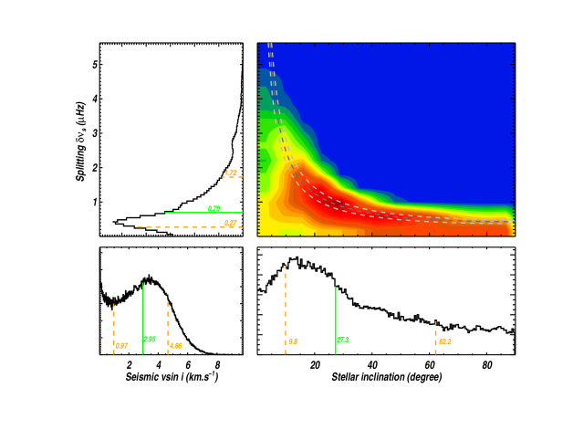
Figure 7: Upper right. Joint posterior probability distribution of the stellar inclination and the rotation for HAT-P-7. Blue represents region of lowest probability. Red areas are of highest probability. Superimposed and using a dark grey dotted line, we show the spectroscopic $v\sin i_{\star}$ from P08 with its $1\sigma$ uncertainty intervals (grey dotted lines). Upper left. Marginalized probability density function for the rotational splitting. Lower right. Marginalized probability density function for the stellar inclination. Lower left. Seismic $v\sin i_{\star}$, inferred using the probability density for the rotational splitting, the inclination and the radius of HAT-P-7.

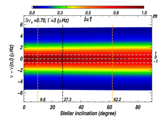
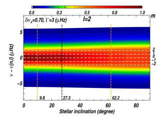
Figure 8: HAT-P-7. Relative power $P(\nu)$ of azimuthal components for $l=1$ (three Lorentzian) and $l=2$ (five Lorentzian) at the median value of the rotational splitting. Width of the Lorentzian is the average mode width ($\Gamma=3\,\mu$Hz). Horizontal dash lines indicate frequencies of the multiplets $m$. Vertical dot-dash lines indicate the credible interval (orange) and the median (black) of the measured inclination (cf. Figure 7). These figures show that because $\delta\nu_{\rm s}\ll\Gamma$, the profile of modes of degree $l=1$ and $l=2$ are almost insensitive to stellar inclination.

Although $\delta\nu_{\rm s}$ is related to the average internal rotation frequency, it provides a good proxy to the surface rotation frequency. Based on this idea, with the radius $R_{\star}$ derived by stellar modelling, we calculated the seismic $v\sin i_{\star}=2\pi R_{\star}\,\delta\nu_{\rm s}\sin i_{\star}$ (cf. Figure 7). We obtained $v\sin i_{\star}=2.95^{+1.71}_{-1.98}$ km s^-1, which is in agreement with $v\sin i_{\star}=3.8\pm 0.5$ km s^-1 obtained by P08.

The degeneracy in solutions due to the correlation between rotation and inclination limits the precision. In our effort to improve our constraint on the inclination angle, $i_{\star}$, we looked for signs of surface rotation by computing the autocorrelation of the timeseries. Solar-like stars may have long-lived surface stellar spots at low latitude that can modulate the light flux periodically, thus revealing the surface rotation period. Unfortunately, HAT-P-7 shows no sign of activity. While this may indicate that the star is not active, this is consistent with our interpretation of the small inclination angle.

5 Asteroseismology of Kepler-25

Kepler-25 is an F star that shows oscillations for which we detected 30 modes of degree $l=0$, $1$ and $l=2$ spanning over 10 radial orders but with amplitudes smaller than HAT-P-7 (Figure 4).

5.1 Fundamental Properties

The precision on the extracted seismic frequencies is lower by approximately a factor two, compared with the case of HAT-P-7. As seen in the échelle diagram (Figure 6) the range of observed frequencies does not allow us to entirely retrieve the oscillation pattern of the modes, which certainly reduces the accuracy of the modelling.

A seismic analysis of Kepler-25 has already been carried out by Huber et al. (2013a) using the empirical scaling relations among mass, radius, effective temperature, the frequency spacing $\Delta\nu$ and frequency at maximum power of the modes, $\nu_{\rm max}$ [see for example Huber et al. (2011) for more details]. They derived $M_{\star}=1.19\pm 0.06\,M_{\odot}$ and $R_{\star}=1.309\pm 0.023\,R_{\odot}$.

For this star, the model with the minimum $\chi^{2}$ is found with surface effect and with an exponent of $b=4.9$. It describes a star with $M_{\star}=1.26\pm 0.03\,M_{\odot}$ and $R_{\star}=1.34\pm 0.01\,R_{\odot}$. This is consistent with the first estimates by Huber et al. (2011). The central hydrogen abundance of $X_{\rm c}=0.329$ corresponds to 46.9% of the initial hydrogen abundance, suggesting a star in the middle of its main sequence stage. The star has a small convective core, extending up to $7\%$ of the stellar radius and an outer convective zone representing $20\%$ of the stellar radius.

5.2 Rotation and Inclination

Figure 9 plots $p(i_{\star},\delta\nu_{\rm s})$, for Kepler-25 as well as their marginalised posterior PDF, $p(\delta\nu_{\rm s})$ and $p(i_{\star})$. We obtain $i_{\star}=\timeform{66D.7}{+\timeform{12D.1}\atop{-\timeform{7D.4}}}$ within a $68\%$ confidence interval. The precision on $i_{\star}$ is much higher than for HAT-P-7, despite a lower signal-to-noise ratio. This is because the rotational splitting is at least twice greater ($\delta\nu_{s}\simeq 1.72\,\mathrm{\mu Hz}$). The multiplets of each degree are disentangled ($\delta\nu_{s}\approx\Gamma\simeq 2.5\mu$Hz), and the mode profile $\mathcal{E}(l,m,i_{\star})$ becomes very sensitive to the stellar inclination (cf. Figure 10).

The radius derived from the best-fit model allows us to directly compare the spectroscopically determined radial velocity, $v\sin i_{\star}$, quoted by Marcy et al. (2014) against our value. As shown in Figure 9, the spectroscopic $v\sin i_{\star}$ is consistent with the maximum location of the joint PDF. Moreover, the rotational kernels of the $l=1$ and $l=2$ modes show that the measured rotational splitting is as much sensitive to the rotation in the convective envelope as into the radiative zone. The modes are however not sensitive to the rotation in the inner convective region. This indicates that the radiative layer and the outer convective region are rotating uniformly, with the same velocity as the surface. Finally, note that $H(n,l,m)$ autocorrelation of the timeseries does not show evidence for stellar activity.

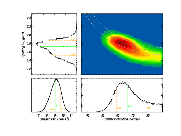
Figure 9: Upper right. Joint posterior probability distribution of the stellar inclination and the rotation for Kepler-25. Blue represents region of lowest probability. Red areas are of highest probability. Superimposed and using a dark grey dotted line, we show the spectroscopic $v\sin i_{\star}$ quoted by Marcy et al. (2014) with its $1\sigma$ uncertainty intervals (grey dotted lines). Upper left. Marginalised probability density function for the rotational splitting. Lower right. Marginalised probability density function for the stellar inclination. Lower left. Seismic $v\sin i_{\star}$, inferred using the probability density for the rotational splitting, the inclination and the radius of Kepler-25.

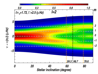
Figure 10: Kepler-25. Relative power $P(\nu)$ of azimuthal components for $l=1$ (three Lorentzian) and $l=2$ (five Lorentzian) at the median value of the rotational splitting. Width of the Lorentzian is the average mode width ($\Gamma=2.5\,\mu$Hz). Horizontal dash lines indicate frequencies of the multiplets $m$. Vertical dotted lines indicate the credible interval (orange) and the median (black) of the measured inclination (cf. Figure 9). The rotation is fast enough to distinguish the Lorentzian profiles of each azimuthal order. This allows an accurate determination of the stellar inclination.

6 Joint Analysis of the HAT-P-7 System

In this section and the next, we combine $i_{\star}$ from asteroseismology and $\lambda$ from the RM effect to constrain the three-dimensional spin–orbit angle $\psi$. Since the seismic $v\sin i_{\star}$ and $\rho_{\star}$ are also complementary to those from the RM effect and transit photometry, we reanalyze the RM effect and the whole available Kepler lightcurves simultaneously, incorporating the constraints on $i_{\star}$, $v\sin i_{\star}$, and $\rho_{\star}$ described in the previous sections as the prior knowledge. The method and results are presented in this section for HAT-P-7 and in the next section for Kepler-25.

For the HAT-P-7 system, the combination of the asteroseismology and Kepler lightcurves provides a unique opportunity to tightly constrain the orbital eccentricity of HAT-P-7b, especially because the occultation (secondary eclipse) is clearly detected for this giant and close-in planet. Therefore, we first describe how the transit and occultation lightcurves constrain the planetary orbit in Section 6.1, before reporting the joint analysis for $\psi$ in Section 6.2.

6.1 Analysis of Transit and Occultation Lightcurves

6.1.1 Data Processing and Revised Ephemeris

In the following analysis, we use the Kepler short-cadence Pre-search Data Conditioned Simple Aperture Photometry (PDCSAP) fluxes through Q0 to Q17 retrieved from the NASA exoplanet archive.

First, lightcurves are detrended and normalized by fitting a third-order polynomial to the out-of-transit fluxes around $\pm 0.5$ days of every transit center. Here, the central time and the duration of each transit are determined from the central time of the first observed transit calculated from the linear ephemeris, $t_{0}$, the orbital period, $P$, and the duration taken from the archive. We iterate the polynomial fit until all the $>5\sigma$ outliers are excluded. In this process, we remove the transits whose baselines cannot be determined reliably due to the data gap around the ingress or egress.

Second, we fit each detrended and normalized transit with the lightcurve model by Ohta et al. (2009) to determine its central time. We fix the planet-to-star radius ratio, $R_{\rm p}/R_{\star}$, the ratio of the semi-major axis to the stellar radius, $a/R_{\star}$, the cosine of the orbital inclination, $\cos i_{\rm orb}$ at those values from the archive, adopt the coefficients for the quadratic limb-darkening law, $u_{1}$ and $u_{2}$, from Jackson et al. (2012), and assume zero orbital eccentricity ($e$). Since only the out-of-transit outliers were removed in the first step, we also iteratively remove in-transit $>5\sigma$ outliers. The resulting transit times are used to phase fold all the transits and to improve the transit parameters and orbital period $P$.

Using these revised transit parameters, we again fit each transit lightcurve for its central time and total duration. Here we assume $e=0$, fix the values of $u_{1}$, $u_{2}$, $a/R_{\star}$, $R_{\rm p}/R_{\star}$, and $P$, and float only central transit time and $\cos i_{\rm orb}$. From these transit times, we calculate the revised ephemeris $t_{0}(\mathrm{BJD})-2454833=121.3585049(49)$ and $P=2.204735427(13)$ days by linear regression. Since we find no systematic TTVs, hereafter we assume that the orbit of HAT-P-7b is described by the strictly periodic Keplerian orbit with $t_{0}$ and $P$ obtained above.

6.1.2 Orbital Eccentricity and Mean Stellar Density from the Phase-folded Transit and Occultation

The top and middle panels of Figure 11 respectively show the transit and occultation lightcurves stacked using the revised ephemeris. The lightcurves are binned into $1$-minute bins and the uncertainty of the flux at the $i$-th bin, $\sigma_{i,\mathrm{MAD}}$, is calculated as $1.4826\times\mathrm{median\ absolute\ deviation}$ divided by the square root of the number of data points in the bin (Bevington, 1969). Solid lines are the best-fit lightcurves obtained from the simultaneous fit to both lightcurves. We use the transit model by Mandel & Agol (2002), and binned model fluxes are calculated by averaging fluxes sampled at 0.1-minute interval. In this figure, the transit and occultation are shifted in time by $t_{{\rm c,\,tra}}$ and $P/2+t_{{\rm c,\,tra}}$, respectively, where $t_{{\rm c,\,tra}}$ is the central time of the phase-folded transit lightcurve. This parameter is introduced to take into account the uncertainty in $t_{0}$, and the best-fit value of $t_{{\rm c,\,tra}}$ is indeed within that uncertainty (see Table 4). In the transit residuals (top panel), we reproduce the anomaly first reported by Morris et al. (2013), who attributed it to the planet-induced gravity darkening.

Since the asymmetry of the planetary orbit alters the relative duration of the transit and occultation, as well as their time interval, one can tightly constrain the orbital eccentricity from the combination of transits and occultations; see equations (33) and (34) in Winn (2011) for instance. The bottom panel of Figure 11 illustrates this subtle effect by comparing the best-fit transit and occultation lightcurves. Here the depth of the occultation is scaled by $\delta$, the occultation depth divided by $(R_{\rm p}/R_{\star})^{2}$, for ease of comparison. In this panel, the egress of the occultation occurs slightly later than that of the transit, while the difference is smaller for their ingresses. In other words, our best-fit model indicates that the occultation duration is longer than the transit one and that the center of occultation deviates from $P/2$. These are most likely due to the asymmetry of the orbit introduced by the slight but non-zero eccentricity, as well as the time delay of $4.5\times 10^{-4}$ days due to the finite speed of light (twice the orbital semi-major axis divided by the speed of light; calculated for $M_{\star}=1.59\,M_{\odot}$). In fact, with the non-zero eccentricity and the above light-travel time included, the simultaneous fit to the phase-folded transit and occultation lightcurves give tight constraints on the planet’s eccentricity, $e\cos\omega=0.00026\pm 0.00015$ and $e\sin\omega=0.0041\pm 0.0022$, where $\omega$ is the argument of periastron measured from the plane of the sky.

Since $e\sin\omega$ and $a/R_{\star}$ are degenerate in determining the transit durations, the tight constraint on $e\sin\omega$ also allows the accurate determination of $a/R_{\star}$, and hence the mean stellar density $\rho_{\star}$ independently from asteroseismology (Seager & Mallén-Ornelas, 2003). We obtain $a/R_{\star}=4.131\pm 0.009$ from the above fit, and then deduce $\rho_{\star}=(0.275\pm 0.002)\times 10^{3}\,\mathrm{kg\,m}^{-3}$ from

$$\rho_{\star}=\frac{3\pi}{GP^{2}}\left(\frac{a}{R_{\star}}\right)^{3}\left(1+\frac{M_{\rm p}}{M_{\star}}\right)^{-1},$$ (8)

where $G$ denotes the gravitational constant, and $M_{\rm p}/M_{\star}\sim 10^{-3}$ can be neglected. This value is larger than $\rho_{\star,\rm s}$ based on the seismic scaling relation by $2.4\sigma$, but consistent with $\rho_{\star,\rm m}$ from the stellar model at the $1\sigma$ level (see Table 3). For this reason, we adopt the constraints from the stellar model as the prior information in the following joint fit. The choice of the prior, however, does not affect the spin–orbit angle determination, but only slightly changes the values of $a/R_{\star}$, $\rho_{\star}$, $\cos i_{\rm orb}$, and $e\sin\omega$. The slight discrepancy between $\rho_{\star}$ from the seismic scaling relation ($\rho_{\star,\rm s}$) and that from transit and occultation implies that the current precision of the Kepler photometry has reached the level that could permit an independent test of the seismic scaling relation for the mean stellar density.

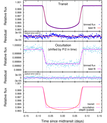
Figure 11: Phase-folded transit (top) and occultation (middle) lightcurves. Points are the binned fluxes ($1\,\mathrm{min}$) and solid lines show the best-fit model lightcurves. Vertical dashed and dotted lines correspond to the four contact points; see figure 2 of Winn (2011) for their definitions. In the bottom panel, we compare the durations and central times of best-fit transit and occultation lightcurves. Occulation is shifted by $P/2$ in time in the middle and the bottom panels, and its depth is scaled by $\delta$ in the bottom panel for ease of comparison.

6.2 Joint Analysis

6.2.1 Method

In this subsection, we report the joint MCMC analysis of phase-folded transit and occultation lightcurves (cf. Section 6.1) and RVs (cf. Section 2.1) making use of the prior constraints on the mean stellar density $\rho_{\star}$, projected stellar rotational velocity $v\sin i_{\star}$, and stellar inclination $i_{\star}$ obtained from asteroseismology in Sections 3–5. As discussed in Section 6.1, the precise constraint on $\rho_{\star}$ (equivalent to that on $a/R_{\star}$) helps to lift the degeneracy between $a/R_{\star}$ and $e\sin\omega$, thus resulting in improved constraints on these two parameters. In addition, $v\sin i_{\star}$ is the key parameter for the RM effect along with $\lambda$, and so the constraints on $v\sin i_{\star}$ help us to better determine $\lambda$ from the observed RM signal. Finally, $i_{\star}$ is crucial in determining the three-dimensional spin–orbit angle $\psi$ via Equation (1), which is the major goal of this paper.

In order to properly handle the possible correlation among $\lambda$, $v\sin i_{\star}$, and $i_{\star}$, we adopt the joint probability distribution for $v\sin i_{\star}$ and $i_{\star}$ as the prior in our MCMC analysis and directly calculate the posterior distribution for $\psi$ by floating $i_{\star}$ as well. It should be noted here that our observables do not determine the sign of $\cos i_{\star}$ or $\cos i_{\rm orb}$, due to the symmetry with respect to the plane of the sky. In order to take into account this inherent degeneracy, we randomly change the sign of the first term in Equation (1) in computing $\psi$. Since the probability distribution of $\rho_{\star}$ is almost independent of those of $v\sin i_{\star}$ and $i_{\star}$, we include the constraint on this parameter as an independent Gaussian with the central value and width of $\rho_{\star,\rm m}$ listed in Table 3.

We adopt the same model (including non-zero eccentricity and light-travel time) for transit and occultation as in Section 6.1. The observed RVs are modeled as

$$v_{\star,\mathrm{model}}(t)=v_{\star,\mathrm{orb}}(t)+v_{\star,\mathrm{RM}}(t)+\gamma_{i}+\dot{\gamma}(t-t_{0}).$$ (9)

Here,

$$v_{\star,\mathrm{orb}}=K_{\star}\left[\cos(\omega+f)+e\cos\omega\right]$$ (10)

is the stellar orbital RVs for the Keplerian orbit, where $K_{\star}$ is the RV semi-amplitude and $f$ is the true anomaly of the planet. The $\gamma_{i}$ ($i=1,2$) are the constant offsets for RVs from Keck/HIRES ($i=1$) and Subaru/HDS ($i=2$), and $\dot{\gamma}$ accounts for the linear trend in the observed RVs in the W09 data set (Winn et al., 2009; Narita et al., 2012; Knutson et al., 2014). Finally, anomalous RVs due to the RM effect, $v_{\star,\mathrm{RM}}$, are modeled following Hirano et al. (2011). The parameters characterizing the RM model include $v\sin i_{\star}$ (projected rotational velocity of the star), $\beta$ (Gaussian dispersion of spectral lines), $\gamma$ (Lorentzian dispersion of spectral lines), $\zeta$ (macroturbulence dispersion of spectral lines), $u_{1\mathrm{RM}}+u_{2\mathrm{RM}}$, and $u_{1\mathrm{RM}}-u_{2\mathrm{RM}}$ (coefficients for the quadratic limb-darkening law in the RM effect). We do not take into account the effect of convective blueshift (Shporer & Brown, 2011), as its typical amplitude ($\sim 1\,\mathrm{m\,s^{-1}}$) is smaller than the (jitter-included) precision of the RVs analyzed here.

We impose the non-seismic priors as well on some of the model parameters. For the ephemeris, we use the Gaussian priors $t_{0}(\mathrm{BJD})-2454833=121.3585049\pm 0.0000049$ and $P=2.204735427\pm 0.000000013\,\mathrm{days}$ obtained from the transit lightcurves. The priors on the RM parameters ($\beta$, $\gamma$, $\zeta$, $u_{1\rm RM}+u_{2\rm RM}$, and $u_{1\rm RM}-u_{2\rm RM}$) are almost the same as in A12. Namely, we fix $\beta=3\,\mathrm{km\,s^{-1}}$ and $\gamma=1\,\mathrm{km\,s^{-1}}$, and assume Gaussian prior $\zeta=5.18\pm 1.5\,\mathrm{km\,s^{-1}}$. We fix the value of $u_{1\mathrm{RM}}-u_{2\mathrm{RM}}$ at $-0.023$ from the tables of Claret (2000) for the Johnson V band and the ATLAS model. The value is obtained using the jktld tool for the parameters $T_{\rm eff}=6350\,\mathrm{K}$, $\log g\,(\mathrm{cgs})=4.07$, and $[{\rm Fe/H}]=0.3$. The value of $u_{1\mathrm{RM}}+u_{2\mathrm{RM}}$ is floated around the tabulated value of $0.70$ assuming the Gaussian prior of width $0.10$. In addition, we impose an additional Gaussian prior on $v\sin i_{\star}$ based on the spectroscopic value in Table 1, because the seismic constraint on this parameter is independent of the spectroscopic $v\sin i_{\star}$. We assume uniform priors for the other $13$ fitting parameters listed in Table 4 (top and middle blocks).

In the joint fit, we assume the same values of stellar jitter as used in the original papers; $9.3\,\mathrm{m\,s^{-1}}$ for the W09 set, $3.8\,\mathrm{m\,s^{-1}}$ for the Keck/HIRES RVs of the N09 set, and $6.0\,\mathrm{m\,s^{-1}}$ for the A12 set. In order to prevent the transit and occultation lightcurves from placing unreasonably tight constraints compared to RVs, we also increase the errors quoted for photometric data (evaluated in Section 6.1.2) as $\sigma_{i}=\sqrt{\sigma_{i,\mathrm{MAD}}^{2}+\sigma_{\rm r}^{2}}$. Here, $\sigma_{\rm r}=5.8\times 10^{-6}$ is a parameter analogous to the RV jitter and chosen so that the reduced $\chi^{2}$ of the lightcurve fit becomes unity. This prescription is also motivated by the following two facts. First, $\sigma_{i,\mathrm{MAD}}$ tends to underestimate the true uncertainty because it neglects the effect of correlated noise. Indeed, when the number of data points is sufficiently large, uncertainties are dominated by the correlated or “red” noise component (Pont et al., 2006). Second, the systematic residuals of the best-fit transit model (top panel of Figure 11) suggest other effects that are not taken into account in our model [e.g., possible planet-induced gravity darkening discussed by Morris et al. (2013)]. Placing too much weights on such features could bias the transit parameters.

6.2.2 Results

Constraints on the system parameters from the joint analysis are summarized in Table 4. The “parameters mainly derived from lightcurves/RVs” are the model (fitted) parameters, while the “derived quantities” are the parameters derived from the model parameters (along with $M_{\star}$ and $R_{\star}$ in Table 3 for $M_{\rm p}$, $R_{\rm p}$, and $\rho_{\rm p}$). While our result is in a reasonable agreement with previous studies (c.f., Morris et al., 2013; Esteves et al., 2013; Van Eylen et al., 2013), it provides two major improvements.

First, we determine the orbital eccentricity of HAT-P-7b essentially from the photometry (i.e., transit, occultation, and asteroseismology) alone. A similar method has recently been employed by Van Eylen et al. (2014) to constrain the planet’s orbital eccentricity using the seismic stellar density (see also Dawson & Johnson, 2012; Kipping, 2014), but here we show that this method is also useful for such a low-eccentricity orbit. Furthermore, our result is even more precise and reliable because it takes into account the independent constraint on $\rho_{\star}$ and $e$ from the occultation lightcurve.

Second, we obtain the probability distribution for the three-dimensional spin–orbit angle $\psi$ in a consistent manner. In the case of HAT-P-7, the constraint on $\psi$ is not very strong because the modest splitting of the azimuthal modes only allows a weak constraint on $i_{\star}$ (see Figure 8). Nevertheless, we find that the peak values of $\psi$ shift towards $90^{\circ}$ compared to those obtained from the “random” $i_{\star}$ (uniform in $\cos i_{\star}$) in all three data sets, as shown in Figure 12. Moreover, the methodology presented here can be applied to other systems, for some of which asteroseismology may be able to tightly constrain $i_{\star}$ unlike HAT-P-7. We will show that this is indeed the case for the Kepler-25 system in the next section.

Table 4: Parameters of the HAT-P-7 System from the Joint Analysis.

Parameter	Value (W09)	Value (N09)	Value (A12)
Parameters mainly derived from lightcurves (transit, occultation, asteroseismology)
$t_{0}(\mathrm{BJD})-2454833$	$121.3585049\pm 0.0000049$
$P$ (days)	$2.204735427\pm 0.000000013$
$e\cos\omega$	$0.00024\pm 0.00020$	$0.00024\pm 0.00020$	$0.00025\pm 0.00020$
$e\sin\omega$	$0.0053_{-0.0021}^{+0.0022}$	$0.0057_{-0.0026}^{+0.0025}$	$0.0049_{-0.0030}^{+0.0026}$
$u_{1}$	$0.3540\pm 0.0034$	$0.3544_{-0.0034}^{+0.0033}$	$0.3545_{-0.0035}^{+0.0034}$
$u_{2}$	$0.1670_{-0.0054}^{+0.0055}$	$0.1663_{-0.0053}^{+0.0055}$	$0.1661_{-0.0055}^{+0.0056}$
$\rho_{\star}$ ($10^{3}\,\mathrm{kg\,m^{-3}}$)	$0.2736\pm 0.0016$	$0.2731_{-0.0018}^{+0.0021}$	$0.2737_{-0.0018}^{+0.0024}$
$\cos i_{\rm orb}$	$0.12149_{-0.00057}^{+0.00056}$	$0.12166_{-0.00068}^{+0.00063}$	$0.12145_{-0.00081}^{+0.00061}$
$R_{\rm p}/R_{\star}$	$0.077589_{-0.000021}^{+0.000020}$	$0.077593\pm 0.000020$	$0.077591_{-0.000021}^{+0.000020}$
$\delta$	$0.01171\pm 0.00010$
$t_{{\rm c,\,tra}}$ (days)	$-0.0000044_{-0.0000042}^{+0.0000041}$
$i_{\star}$ (∘)	$31_{-16}^{+33}$	$33_{-20}^{+34}$	$33_{-20}^{+34}$
Parameters mainly derived from RVs
$K_{\star}$ ($\mathrm{m\,s^{-1}}$)	$211.7\pm 2.3$	$213.2\pm 1.8$	$214.0\pm 4.6$
$\gamma_{1}$ ($\mathrm{m\,s^{-1}}$)	$-15.5\pm 3.0$	$-37.5\pm 1.5$	$10.4_{-1.6}^{+1.5}$
$\gamma_{2}$ ($\mathrm{m\,s^{-1}}$)	$-9.7\pm 1.7$	$-16.9\pm 1.4$	–
$\dot{\gamma}$ ($\mathrm{m\,s^{-1}\,yr^{-1}}$)	$21.5\pm 2.5$	–	–
$\lambda$ (∘)	$186_{-11}^{+10}$	$220.3_{-9.3}^{+8.2}$	$157_{-13}^{+14}$
$v\sin i_{\star}$ ($\mathrm{km\,s^{-1}}$)	$4.15_{-0.39}^{+0.38}$	$3.17\pm 0.33$	$3.17_{-0.34}^{+0.33}$
$\beta$ ($\mathrm{km\,s^{-1}}$)	$3.0$ (fixed)
$\gamma$ ($\mathrm{km\,s^{-1}}$)	$1.0$ (fixed)
$\zeta$ ($\mathrm{km\,s^{-1}}$)	$5.3\pm 1.5$	$5.5\pm 1.5$	$5.5\pm 1.5$
$u_{1\mathrm{RM}}+u_{2\mathrm{RM}}$	$0.70\pm 0.10$
$u_{1\mathrm{RM}}-u_{2\mathrm{RM}}$	$-0.23$ (fixed)
Derived quantities
$\psi$ (∘)	$122_{-18}^{+30}$	$115_{-16}^{+19}$	$120_{-18}^{+26}$
$a/R_{\star}$	$4.1269_{-0.0078}^{+0.0082}$	$4.1245_{-0.0092}^{+0.0103}$	$4.1277_{-0.0090}^{+0.0121}$
transit impact parameter ($R_{\star}$)	$0.4987\pm 0.0013$	$0.4989\pm 0.0013$	$0.4988_{-0.0014}^{+0.0013}$
$T_{14,\mathrm{tra}}$ (days)	$0.164301\pm 0.000022$	$0.164303\pm 0.000023$	$0.164300\pm 0.000023$
$T_{23,\mathrm{tra}}$ (days)	$0.133042_{-0.000048}^{+0.000049}$	$0.133034_{-0.000048}^{+0.000047}$	$0.133037_{-0.000048}^{+0.000052}$
$T_{\mathrm{tra}}$ (days)	$0.148672_{-0.000024}^{+0.000025}$	$0.148668\pm 0.000024$	$0.148669_{-0.000024}^{+0.000025}$
occultation impact parameter ($R_{\star}$)	$0.5040_{-0.0023}^{+0.0022}$	$0.5047_{-0.0028}^{+0.0025}$	$0.5039_{-0.0033}^{+0.0024}$
$T_{14,\mathrm{occ}}$ (days)	$0.16555_{-0.00050}^{+0.00051}$	$0.16566_{-0.00061}^{+0.00058}$	$0.16547_{-0.00070}^{+0.00060}$
$T_{23,\mathrm{occ}}$ (days)	$0.13385_{-0.00033}^{+0.00034}$	$0.13392_{-0.00040}^{+0.00039}$	$0.13379_{-0.00046}^{+0.00041}$
$T_{\mathrm{occ}}$ (days)	$0.14970_{-0.00041}^{+0.00042}$	$0.14979_{-0.00051}^{+0.00048}$	$0.14963_{-0.00058}^{+0.00050}$
occultation depth (ppm)	$70.5\pm 0.6$
$M_{\rm p}(M_{\rm J})$	$1.86\pm 0.03$	$1.87\pm 0.03$	$1.88\pm 0.05$
$R_{\rm p}(R_{\rm J})$	$1.526\pm 0.008$
$\rho_{\rm p}$ ($10^{3}\,\mathrm{kg\,m^{-3}}$)	$0.65\pm 0.01$	$0.66\pm 0.01$	$0.66\pm 0.02$
Note — The quoted best-fit values are the medians of their MCMC posteriors, and uncertainties exclude 15.87% of values at upper and lower extremes. The $T_{ij}$ ($i,j=1,2,3,4$) is the duration between the two contact points $i$ and $j$ [see figure 2 of Winn (2011) for their definitions], and $T=(T_{14}+T_{23})/2$. The subscript “tra” refers to transits and “occ” to occultations.

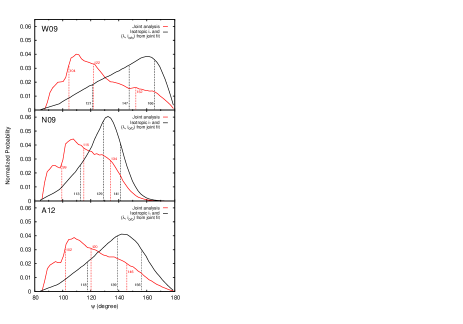
Figure 12: Probability distributions for the three-dimensional spin–orbit angle $\psi$ of HAT-P-7b for the W09 (top), N09 (middle), and A12 (bottom) data sets. Solid red lines show the posteriors from the joint analysis, while the black ones are the probability distributions obtained from uniform $\cos i_{\star}$ and the posteriors of $\lambda$ and $i_{\rm orb}$ from the joint analysis (Table 4). The median, $1\sigma$ lower limit, and $1\sigma$ upper limit for each distribution are shown in vertical dotted lines. A small bump around $\psi\approx 95^{\circ}$ in each panel originates from the fact that each posterior shown here is the superposition of the two inherently degenerate configurations with the opposite signs of $\cos i_{\star}\cos i_{\rm orb}$; see the discussion in the second paragraph of Section 6.2.1.

7 Joint Analysis of the Kepler-25 System

7.1 Method

We repeat almost the same analysis for Kepler-25c as in Section 6. There are, however, several differences in the lightcurve and RV analyses as described below, mainly due to the multiplicity of the Kepler-25 system and relatively small signal-to-noise ratio of the Kepler-25c’s transit:

1. We phase-fold the transits using the actually observed transit times rather than those calculated from the linear ephemeris. This is because the transit times of Kepler-25c ($P=12.7$ days) exhibit significant TTVs due to the proximity to the $2:1$ mean-motion resonance with Kepler-25b ($P=6.2$ days). This is why we do not allow $t_{{\rm c,\,tra}}$, the central time of the phase-folded transit, to be a free parameter. We adopt $\sigma_{\rm r}=1.6\times 10^{-5}$ based on the $\chi^{2}$ of the lightcurve fit.

2. The occultation of Kepler-25c was not detected and not taken into account in the following analysis.

3. As the quality of the transit lightcurve of Kepler-25c is not so good as that of HAT-P-7b, we could not determine the limb-darkening coefficients very well. For this reason, we impose the prior $u_{1}-u_{2}=-0.0015\pm 0.50$ based on the tables of Claret (2000), and choose $u_{1}+u_{2}$ and $u_{1}-u_{2}$, instead of $u_{1}$ and $u_{2}$, as free parameters. We made sure that the choice of the confidence interval for $u_{1}-u_{2}$ does not affect the constraint on $\psi$.

4. In order to take into account the other planets in the RV fit, we allow the orbital semi-amplitude $K_{\star}$ and RV offset $\gamma$ for each of the nights in 2011 and 2012 to be free parameters, as in A13. RV jitters are fixed at $3.3\,\mathrm{m\,s^{-1}}$.

5. We do not fit the orbital eccentricity but fix $e=0$, because we do not analyze the occultation nor RVs throughout the orbit (Marcy et al., 2014).

6. We assume the independent Gaussian priors $u_{1\mathrm{RM}}+u_{2\mathrm{RM}}=0.69\pm 0.10$ and $\zeta=4.85\pm 1.5\,\mathrm{km\,s^{-1}}$ from A13, and fix $u_{1\mathrm{RM}}-u_{2\mathrm{RM}}=-0.0297$ from the tables of Claret (2000).

7.2 Results

In the case of the Kepler-25 system, the uncertainty in $\psi$ is significantly reduced by virtue of the seismic information. This situation is clearly illustrated in Figure 13, which compares the posterior probability distribution for $\psi$ from the joint fit (solid red line) to that based on $\lambda$ and $i_{\rm orb}$ from the joint fit and the uniform $\cos i_{\star}$ (solid black line). The corresponding system parameters are summarized in Table 5. They are basically consistent with those obtained by A13, except for the increased precision in the transit parameters.

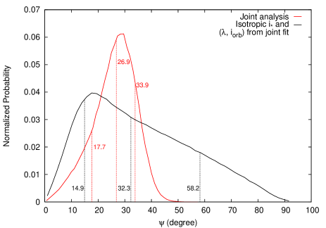
Figure 13: Probability distributions for the three-dimensional spin–orbit angle $\psi$ of Kepler-25c. The solid red line shows the posterior from the joint analysis, while the black one is the probability distribution obtained from $\lambda$ and $i_{\rm orb}$ in Table 5 and uniform $\cos i_{\star}$. The median, $1\sigma$ lower limit, and $1\sigma$ upper limit for each distribution are shown in vertical dotted lines.

Interestingly, our result suggests a spin–orbit misalignment for Kepler-25c with more than $2\sigma$ significance. In order to check the robustness of this result, we also calculate the probability distribution of $\psi$ for the seismic $i_{\star}$ and an independent Gaussian $\lambda=-\timeform{0D.5}\pm\timeform{5D.7}$ from the Doppler tomography. We obtain $\psi=\timeform{23D.7}_{-\timeform{11D.3}}^{+\timeform{8D.0}}$ in this case, which still points to the spin–orbit misalignment marginally. If confirmed, this will be the first example of the spin–orbit misalignment in the multi-transiting system around a main-sequence star. The implication of this result will be discussed in Section 8.2.

Table 5: Parameters of the Kepler-25 System from the Joint Analysis (see also the note in Table 4).

Parameter	Value (A13)
Parameters mainly derived from lightcurves
(transit, asteroseismology)
$t_{0}(\mathrm{BJD})-2454833$	$127.646558_{-0.000094}^{+0.000096}$
$P$ (days)	$12.7203724_{-0.0000013}^{+0.0000014}$
$u_{1}+u_{2}$	$0.550\pm 0.018$
$u_{1}-u_{2}$	$-0.27\pm 0.44$
$\rho_{\star}$ ($10^{3}\,\mathrm{kg\,m^{-3}}$)	$0.733_{-0.012}^{+0.013}$
$\cos i_{\rm orb}$	$0.04788_{-0.00038}^{+0.00036}$
$R_{\rm p}/R_{\star}$	$0.03590_{-0.00046}^{+0.00054}$
$i_{\star}$ (∘)	$65.4_{-6.4}^{+10.6}$
Parameters mainly derived from RVs
$K_{\star,2011}$ ($\mathrm{m\,s^{-1}}$)	$-13\pm 22$
$K_{\star,2012}$ ($\mathrm{m\,s^{-1}}$)	$-37\pm 30$
$\gamma_{2011}$ ($\mathrm{m\,s^{-1}}$)	$-3.5\pm 1.3$
$\gamma_{2012}$ ($\mathrm{m\,s^{-1}}$)	$2.0\pm 1.4$
$\lambda$ (∘)	$9.4\pm 7.1$
$v\sin i_{\star}$ ($\mathrm{km\,s^{-1}}$)	$9.34_{-0.39}^{+0.37}$
$\beta$ ($\mathrm{km\,s^{-1}}$)	$3.0$ (fixed)
$\gamma$ ($\mathrm{km\,s^{-1}}$)	$1.0$ (fixed)
$\zeta$ ($\mathrm{km\,s^{-1}}$)	$4.9\pm 1.5$
$u_{1\mathrm{RM}}+u_{2\mathrm{RM}}$	$0.69\pm 0.10$
$u_{1\mathrm{RM}}-u_{2\mathrm{RM}}$	$-0.0297$ (fixed)
Derived quantities
$\psi$ (∘)	$26.9_{-9.2}^{+7.0}$
$a/R_{\star}$	$18.44\pm 0.11$
transit impact parameter ($R_{\star}$)	$0.8826\pm 0.0018$
$T_{14,\mathrm{tra}}$ (days)	$0.11925\pm 0.00025$
$T_{23,\mathrm{tra}}$ (days)	$0.08528_{-0.00069}^{+0.00065}$
$T_{\mathrm{tra}}$ (days)	$0.10226_{-0.00037}^{+0.00036}$

8 Discussion

8.1 HAT-P-7

From asteroseismology alone, we obtain $i_{\star}=\timeform{27D}_{-\timeform{18D}}^{+\timeform{35D}}$ for HAT-P-7 (Figure 7). This constraint, combined with the Kepler lightcurves and the three independent RM measurements, yields $\psi=\timeform{122D}_{\timeform{-18D}}^{\timeform{+30D}}$ and $i_{\star}=\timeform{31D}^{+\timeform{33D}}_{-\timeform{16D}}$, $\psi=\timeform{115D}_{\timeform{-16D}}^{\timeform{+19D}}$ and $i_{\star}=\timeform{33D}^{+\timeform{34D}}_{-\timeform{20D}}$, and $\psi=\timeform{120D}_{\timeform{-18D}}^{\timeform{+26D}}$ and $i_{\star}=\timeform{33D}_{-\timeform{20D}}^{+\timeform{34D}}$ for the RVs from W09, N09, and A12, respectively (Figure 12 and Table 4). Although the resulting constraints are not very strong due to the modest splittings of azimuthal modes (see Figure 8), our results suggest that the orbit of HAT-P-7b is closer to the polar configuration rather than retrograde as $\lambda$ may imply.

It is worth noting that the suggested discrepancies in $\lambda$ and $v\sin i_{\star}$ in three data sets (cf. Section 2.1) still persist in our analysis. For a fair comparison with the A12 result, we repeat the same analyses for the W09 and N09 data only including RVs taken over the same night, but the values of $\lambda$ and $v\sin i_{\star}$ do not change significantly. Since we have used the same model of the RM effect and the same priors from the Kepler photometry for the three sets of data, our results confirm that the discrepancy comes from the RV data themselves. As A12 discussed, such a discrepancy may originate from some physics that is not included in the current model of the RM effect, but its origin is beyond the scope of this paper.

As a by-product of the spin–orbit analysis, we have found that HAT-P-7b has a small but non-zero orbital eccentricity, $e=0.005\pm 0.001$ (weighted mean of the three data sets), which is consistent with $e=0.0055_{-0.0033}^{+0.007}$ obtained by Knutson et al. (2014). Our constraint on $e$ comes from the duration and mid-time of the occultation of HAT-P-7b relative to those of the transit, along with the constraint on the mean stellar density $\rho_{\star}$ from asteroseismology. This approach is justified by the fact that $\rho_{\star}$ from the transit and occultation alone shows a reasonable agreement with the model stellar density $\rho_{\star,\rm m}$ derived independently from asteroseismology. The origin of this non-zero $e$ may deserve further theoretical consideration because the tides are expected to damp $e$ rapidly for such a close-in planet like HAT-P-7b.

8.2 Kepler-25

For Kepler-25, we obtain $i_{\star}=\timeform{65D.4}_{-\timeform{6D.4}}^{+\timeform{10D.6}}$ from the joint analysis. This is slightly better than $i_{\star}=\timeform{66D.7}^{+\timeform{12D.1}}_{-\timeform{7D.4}}$ from asteroseismology alone (Figure 9), mainly due to the prior on $v\sin i_{\star}$ from spectroscopy. The constraint on $i_{\star}$ is better than HAT-P-7 despite the lower signal-to-noise ratio, because of the greater rotational splitting (see Figure 10). This allows us to tightly constrain the spin–orbit angle of Kepler-25c as $\psi=\timeform{26D.9}_{-\timeform{9D.2}}^{+\timeform{7D.0}}$ (Figure 13). Our finding is important in two aspects; 1) this is the first quantitative measurement of $\psi$, instead of $\lambda$, for multi-planetary systems, except for the Solar system. 2) Kepler-25 is the first system that exhibits the significant spin–orbit misalignment among the multi-transiting systems with a main-sequence host star, while it is the second example if we consider the systems with a red-giant host star, Kepler-56.

The spin–orbit misalignment in systems with multiple transiting planets is particularly interesting for the following reason. Considering the transit probabilities of multiple planets, planets’ orbital planes are likely to be coplanar in multi-transiting systems, and hence presumably trace their natal protoplanetary disks. The spin–orbit misalignment in such systems, therefore, could be a clue to the processes that tilt a stellar spin relative to its protoplanetary disk (e.g., Bate et al., 2010; Lai et al., 2011; Batygin, 2012).

In this context, the orbital inclinations of the other two planets (Kepler-25b and Kepler-25d) relative to that of Kepler-25c would help the interpretation of the observed misalignment. They may be constrained from the analysis of TTVs and Transit Duration Variations (TDVs), along with orbital RVs to constrain the orbit of the outer non-transiting planet d. In this paper, we did not model these phenomena because our main concern is the determination of the spin–orbit angle. It should be noted, however, that the independent information on $\rho_{\star}$ from asteroseismology benefits the TTV analysis as well because TTVs are sensitive to the mean stellar density and orbital eccentricity of the planets (e.g., Sanchis-Ojeda et al., 2012; Masuda, 2014).

It is also interesting to note that both HAT-P-7 and Kepler-25 are relatively hot stars with $T_{\rm eff}\gtrsim 6300\,\mathrm{K}$ and in line with the observed trend that the spin–orbit misalignments are preferentially found around stars with $T_{\rm eff}>6250\,\mathrm{K}$ (Winn et al., 2010). Although Rogers et al. (2012) suggested that temporal variations of the stellar rotation due to internal gravity waves could explain this empirical trend, we found no evidence to support this scenario for the two systems. Regarding HAT-P-7, we compared the rotational splitting from Figure 7 with that from Q0 to Q2 (results from the study of Oshagh et al., 2013), but found no evidence of significant variations. Although results using only Q0 to Q2 have large uncertainties, this may indicate that the rotation remains constant over time. Moreover, we tightly constrained the rotation of Kepler-25 and showed that outer layers certainly rotate at constant velocity. This is incompatible with the scenario suggested by Rogers et al. (2012).

9 Summary

The major purpose of the present paper is two-fold. The first is to develop and describe a detailed methodology of determining the three-dimensional spin–orbit angle $\psi$ for transiting planetary systems. The other is to demonstrate the power of the methodology by applying to the two specific systems, HAT-P-7 and Kepler-25.

The application of asteroseismology to exoplanetary systems is now becoming popular. It is particularly useful in determining the stellar inclination $i_{\star}$ with respect to the line-of-sight. Combined with the orbital inclination $i_{\rm orb}$ determined for transiting systems, and with the projected spin-orbit angle $\lambda$ via the spectroscopic observation of the Rossiter-McLaughlin effect, the joint analysis presented in this paper indeed enables the determination of $\psi$, rather than $\lambda$. While the observed distribution of $\lambda$ for more than 70 transiting systems [e.g., figure 7 of Xue et al. (2014)] already put tight constraints on planetary migration scenarios, that of $\psi$ is even more useful because it is free from the projection effect. As we discussed, HAT-P-7 seems to host a polar-orbit planet instead of a retrograde one as naively suspected from the observed $\lambda\approx\timeform{180D}$. The determination of $\psi$ is also important for multi-transiting planetary systems where all the planets are supposed to share the same orbital plane; large $\psi$ in such a system indicates that the stellar obliquity experiences significant tilt with respect to the protoplanetary disk that would be the orbital plane of the planets. This turned out to be the case for Kepler-25 as we discussed in the previous section. While it may be premature to consider the statistics at this point, it is tempting to note that two out of the six multi-transiting systems with measured spin–orbit angles are shown to be significantly misaligned. The misaligned cases are Kepler-25c ($\psi=\timeform{26D.9}_{-\timeform{9D.2}}^{+\timeform{7D.0}}$) and Kepler-56 ($i_{\star}=\timeform{47D}\pm\timeform{6D}$, Huber et al., 2013b), while the aligned cases are Kepler-30 ($\lambda\lesssim\timeform{10D}$, Sanchis-Ojeda et al., 2012), Kepler-50 and Kepler-65 ($i_{\star}=\timeform{82D}^{+\timeform{8D}}_{-\timeform{7D}}$ and $i_{\star}=\timeform{81D}^{+\timeform{9D}}_{-\timeform{16D}}$, Chaplin et al., 2013) and Kepler-89d (KOI-94d) with $\lambda=-\timeform{6D}^{+\timeform{13D}}_{-\timeform{11D}}$ (Hirano et al., 2012b) or $-\timeform{11D}\pm\timeform{11D}$ (A13). Even if the spin–orbit misalignment is rare, the physical mechanism for its origin is an interesting theoretical question. If it indeed turns out to be fairly common, it will pose a serious challenge to all viable theories of the formation and evolution of multi-planetary systems.

In addition to the determination of $\psi$, the joint analysis improves the accuracy and precision of numerous system parameters for a specific target. In turn, any discrepancy among the separate analyses strongly points to a certain physical process which needs to be taken into account in the detailed modeling. This would open a new window for the exploration of the origin and evolution of planetary systems.

We are grateful to Simon Albrecht and Josh Winn for providing us with the radial velocity data of Kepler-25. We thank NASA and the Kepler team for their revolutionary data. O.B. is supported by Japan Society for Promotion of Science (JSPS) Fellowship for Research (No. 25-13316). K.M. is supported by JSPS Research Fellowships for Young Scientists (No. 26-7182) and by the Leading Graduate Course for Frontiers of Mathematical Sciences and Physics. Y.S. gratefully acknowledges the support from the Grant-in Aid for Scientific Research by JSPS (No. 24340035).

References

- Aerts et al. (2010) Aerts, C., Christensen-Dalsgaard, J., & Kurtz, W. 2010, Asteroseismology, 1st edn. (Springer Science)
- Albrecht et al. (2013) Albrecht, S., Winn, J. N., Marcy, G. W., Howard, A. W., Isaacson, H., & Johnson, J. A. 2013, ApJ, 771, 11 (A13)
- Albrecht et al. (2012) Albrecht, S., et al. 2012, ApJ, 757, 18 (A12)
- Appourchaux et al. (2008) Appourchaux, T., et al. 2008, A&A, 488, 705
- Appourchaux et al. (2012) —. 2012, A&A, 543, A54
- Asplund et al. (2009) Asplund, M., Grevesse, N., Sauval, A. J., & Scott, P. 2009, ARA&A, 47, 481
- Baglin et al. (2006a) Baglin, A., Auvergne, M., Barge, P., Deleuil, M., Catala, C., Michel, E., Weiss, W., & COROT Team. 2006a, in ESA Special Publication, Vol. 1306, ESA Special Publication, ed. M. Fridlund, A. Baglin, J. Lochard, & L. Conroy, 33
- Baglin et al. (2006b) Baglin, A., et al. 2006b, in COSPAR Meeting, Vol. 36, 36th COSPAR Scientific Assembly, 3749
- Ballot (2010) Ballot, J. 2010, Astronomische Nachrichten, 331, 933
- Bate et al. (2010) Bate, M. R., Lodato, G., & Pringle, J. E. 2010, MNRAS, 401, 1505
- Batygin (2012) Batygin, K. 2012, Nature, 491, 418
- Bazot et al. (2005) Bazot, M., Vauclair, S., Bouchy, F., & Santos, N. C. 2005, A&A, 440, 615
- Benomar et al. (2009a) Benomar, O., Appourchaux, T., & Baudin, F. 2009a, A&A, 506, 15
- Benomar et al. (2009b) Benomar, O., et al. 2009b, A&A, 507, L13
- Benomar et al. (2013) —. 2013, ApJ, 767, 158
- Benomar et al. (2014) —. 2014, ApJ, 781, L29
- Bevington (1969) Bevington, P. R. 1969, Data reduction and error analysis for the physical sciences
- Borucki et al. (2010) Borucki, W. J., et al. 2010, Science, 327, 977
- Carter et al. (2012) Carter, J. A., et al. 2012, Science, 337, 556
- Chaplin et al. (2013) Chaplin, W. J., et al. 2013, ApJ, 766, 101
- Christensen-Dalsgaard (2008) Christensen-Dalsgaard, J. 2008, Ap&SS, 316, 113
- Christensen-Dalsgaard et al. (2010) Christensen-Dalsgaard, J., et al. 2010, ApJ, 713, L164
- Claret (2000) Claret, A. 2000, A&A, 363, 1081
- Collier Cameron et al. (2010) Collier Cameron, A., Bruce, V. A., Miller, G. R. M., Triaud, A. H. M. J., & Queloz, D. 2010, MNRAS, 403, 151
- Dawson & Johnson (2012) Dawson, R. I., & Johnson, J. A. 2012, ApJ, 756, 122
- Esteves et al. (2013) Esteves, L. J., De Mooij, E. J. W., & Jayawardhana, R. 2013, ApJ, 772, 51
- Fabrycky & Tremaine (2007) Fabrycky, D., & Tremaine, S. 2007, ApJ, 669, 1298
- García et al. (2011a) García, R. A., Salabert, D., Ballot, J., Sato, K., Mathur, S., & Jiménez, A. 2011a, Journal of Physics Conference Series, 271, 012049
- García et al. (2011b) García, R. A., et al. 2011b, MNRAS, 414, L6
- Gizon & Solanki (2003) Gizon, L., & Solanki, S. K. 2003, ApJ, 589, 1009
- Gizon et al. (2013) Gizon, L., et al. 2013, Proceedings of the National Academy of Science, 110, 13267
- Grec et al. (1983) Grec, G., Fossat, E., & Pomerantz, M. A. 1983, Sol. Phys., 82, 55
- Guzik et al. (2014) Guzik, J. A., Chaplin, W. J., Handler, G., & Pigulski, A., eds. 2014, IAU Symposium, Vol. 301, Precision Asteroseismology
- Harvey (1985) Harvey, J. 1985, ESA SP, 235, 199
- Hirano et al. (2012a) Hirano, T., Sanchis-Ojeda, R., Takeda, Y., Narita, N., Winn, J. N., Taruya, A., & Suto, Y. 2012a, ApJ, 756, 66
- Hirano et al. (2010) Hirano, T., Suto, Y., Taruya, A., Narita, N., Sato, B., Johnson, J. A., & Winn, J. N. 2010, ApJ, 709, 458
- Hirano et al. (2011) Hirano, T., Suto, Y., Winn, J. N., Taruya, A., Narita, N., Albrecht, S., & Sato, B. 2011, ApJ, 742, 69
- Hirano et al. (2012b) Hirano, T., et al. 2012b, ApJ, 759, L36
- Huber et al. (2011) Huber, D., et al. 2011, ApJ, 743, 143
- Huber et al. (2013a) —. 2013a, ApJ, 767, 127
- Huber et al. (2013b) —. 2013b, Science, 342, 331
- Jackson et al. (2012) Jackson, B. K., Lewis, N. K., Barnes, J. W., Drake Deming, L., Showman, A. P., & Fortney, J. J. 2012, ApJ, 751, 112
- Jeffreys (1961) Jeffreys, H. 1961, Theory of Probability, 3rd edn. (Oxford, England: Oxford)
- Kipping (2014) Kipping, D. M. 2014, MNRAS, 440, 2164
- Kjeldsen et al. (2008) Kjeldsen, H., Bedding, T. R., & Christensen-Dalsgaard, J. 2008, ApJ, 683, L175
- Knutson et al. (2014) Knutson, H. A., et al. 2014, ApJ, 785, 126
- Lai (2012) Lai, D. 2012, MNRAS, 423, 486
- Lai et al. (2011) Lai, D., Foucart, F., & Lin, D. N. C. 2011, MNRAS, 412, 2790
- Lebreton & Montalbán (2009) Lebreton, Y., & Montalbán, J. 2009, in IAU Symposium, Vol. 258, IAU Symposium, ed. E. E. Mamajek, D. R. Soderblom, & R. F. G. Wyse, 419–430
- Mandel & Agol (2002) Mandel, K., & Agol, E. 2002, ApJ, 580, L171
- Marcy et al. (2014) Marcy, G. W., et al. 2014, ApJS, 210, 20
- Masuda (2014) Masuda, K. 2014, ApJ, 783, 53
- Masuda et al. (2013) Masuda, K., Hirano, T., Taruya, A., Nagasawa, M., & Suto, Y. 2013, ApJ, 778, 185
- McLaughlin (1924) McLaughlin, D. B. 1924, ApJ, 60, 22
- Metcalfe et al. (2012) Metcalfe, T. S., et al. 2012, ApJ, 748, L10
- Monteiro et al. (1994) Monteiro, M. J. P. F. G., Christensen-Dalsgaard, J., & Thompson, M. J. 1994, A&A, 283, 247
- Morris et al. (2013) Morris, B. M., Mandell, A. M., & Deming, D. 2013, ApJ, 764, L22
- Nagasawa & Ida (2011) Nagasawa, M., & Ida, S. 2011, ApJ, 742, 72
- Nagasawa et al. (2008) Nagasawa, M., Ida, S., & Bessho, T. 2008, ApJ, 678, 498
- Narita et al. (2009) Narita, N., Sato, B., Hirano, T., & Tamura, M. 2009, PASJ, 61, L35 (N09)
- Narita et al. (2012) Narita, N., et al. 2012, PASJ, 64, L7
- Nelder & Mead (1965) Nelder, J. A., & Mead, R. 1965, The Computer Journal, 7, 308
- Ohta et al. (2005) Ohta, Y., Taruya, A., & Suto, Y. 2005, ApJ, 622, 1118
- Ohta et al. (2009) —. 2009, ApJ, 690, 1
- Oshagh et al. (2013) Oshagh, M., Grigahcène, A., Benomar, O., Dupret, M.-A., Monteiro, M. J. P. F. G., Scuflaire, R., & Santos, N. C. 2013, in Astrophysics and Space Science Proceedings, Vol. 31, Stellar Pulsations: Impact of New Instrumentation and New Insights, ed. J. C. Suárez, R. Garrido, L. A. Balona, & J. Christensen-Dalsgaard, 227
- Pál et al. (2008) Pál, A., et al. 2008, ApJ, 680, 1450 (P08)
- Paxton et al. (2011) Paxton, B., Bildsten, L., Dotter, A., Herwig, F., Lesaffre, P., & Timmes, F. 2011, ApJS, 192, 3
- Paxton et al. (2013) Paxton, B., et al. 2013, ApJS, 208, 4
- Pont et al. (2006) Pont, F., Zucker, S., & Queloz, D. 2006, MNRAS, 373, 231
- Queloz et al. (2000) Queloz, D., Eggenberger, A., Mayor, M., Perrier, C., Beuzit, J. L., Naef, D., Sivan, J. P., & Udry, S. 2000, A&A, 359, L13
- Reese et al. (2006) Reese, D., Lignières, F., & Rieutord, M. 2006, A&A, 455, 621
- Rogers et al. (2012) Rogers, T. M., Lin, D. N. C., & Lau, H. H. B. 2012, ApJ, 758, L6
- Rossiter (1924) Rossiter, R. A. 1924, ApJ, 60, 15
- Roxburgh & Vorontsov (2003) Roxburgh, I. W., & Vorontsov, S. V. 2003, A&A, 411, 215
- Sanchis-Ojeda et al. (2012) Sanchis-Ojeda, R., et al. 2012, Nature, 487, 449
- Schlaufman (2010) Schlaufman, K. C. 2010, ApJ, 719, 602
- Seager & Mallén-Ornelas (2003) Seager, S., & Mallén-Ornelas, G. 2003, ApJ, 585, 1038
- Shibahashi & Lynas-Gray (2013) Shibahashi, H., & Lynas-Gray, A. E., eds. 2013, Astronomical Society of the Pacific Conference Series, Vol. 479, Progress in Physics of the Sun and Stars
- Shibahashi et al. (2012) Shibahashi, H., Takata, M., & Lynas-Gray, A. E., eds. 2012, Astronomical Society of the Pacific Conference Series, Vol. 462, Progress in Solar/Stellar Physics with Helio- and Asteroseismology
- Shporer & Brown (2011) Shporer, A., & Brown, T. 2011, ApJ, 733, 30
- Steffen et al. (2012) Steffen, J. H., et al. 2012, MNRAS, 421, 2342
- Unno et al. (1989) Unno, W., Osaki, Y., Ando, H., Saio, H., & Shibahashi, H. 1989, Nonradial Oscillations of Stars (University Tokyo Press)
- Van Eylen et al. (2012) Van Eylen, V., Kjeldsen, H., Christensen-Dalsgaard, J., & Aerts, C. 2012, Astronomische Nachrichten, 333, 1088
- Van Eylen et al. (2013) Van Eylen, V., Lindholm Nielsen, M., Hinrup, B., Tingley, B., & Kjeldsen, H. 2013, ApJ, 774, L19
- Van Eylen et al. (2014) Van Eylen, V., et al. 2014, ApJ, 782, 14
- Vorontsov (1988) Vorontsov, S. V. 1988, in IAU Symposium, Vol. 123, Advances in Helio- and Asteroseismology, ed. J. Christensen-Dalsgaard & S. Frandsen, 151
- Walker et al. (2003) Walker, G., et al. 2003, PASP, 115, 1023
- White et al. (2012) White, T. R., et al. 2012, ApJ, 751, L36
- Winn (2011) Winn, J. N. 2011, in Exoplanets, ed. S. Seager (Tucson, AZ: University of Arizona Press), 55–77
- Winn et al. (2010) Winn, J. N., Fabrycky, D., Albrecht, S., & Johnson, J. A. 2010, ApJ, 718, L145
- Winn et al. (2009) Winn, J. N., Johnson, J. A., Albrecht, S., Howard, A. W., Marcy, G. W., Crossfield, I. J., & Holman, M. J. 2009, ApJ, 703, L99 (W09)
- Winn et al. (2005) Winn, J. N., et al. 2005, ApJ, 631, 1215
- Xue et al. (2014) Xue, Y., Suto, Y., Taruya, A., Hirano, T., Fujii, Y., & Masuda, K. 2014, ApJ, 784, 66