Effective and simple VWAP options pricing model

Abstract

Volume weighted average price (VWAP) options are a popular security type in many countries, but despite their popularity very few pricing models have been developed so far for VWAP options. This can be explained by the fact that the VWAP pricing problem is set in an incomplete market since there is no underlying with which to hedge the volume risk, and hence there is no uniquely defined price. Any price, which is obtained will include a market price of volume risk which must be determined from the corresponding volume statistics. Our analysis strongly supports the hypothesis that the empirical volume statistics of ASX equities can be described reasonably well by fitted gamma distributions. Based on this observation we suggest a simple gamma process-based model that allows for the exact analytic pricing of VWAP options in a rather straightforward way.

1 Introduction

The volume weighted average price (VWAP) occurs frequently in finance. It is an average price which gives more weight to periods of high trading than to periods of low trading in its calculation. A broker’s daily performance is frequently measured against the VWAP and it is becoming increasingly popular for institutional investors to place buy and sell orders at the VWAP. The VWAP also appears in Australian taxation law as part of determining the prices of share buy-backs in publicly listed companies (Woellner et al. (2009)).

Most of the existing literature on VWAP focuses on strategies and algorithms to execute orders as close as possible to the VWAP price (see e.g. Konishi (2002), Bialkowski et al. (2008), Fuh et al. (2010), Frei & Westray (2013)). On the other hand, surprisingly few results on actual pricing methodologies related to VWAP options have been published (Stace (2007), Novikov et al. (2014)). This can be explained by pointing out that the VWAP pricing problem is set in an incomplete market since there is no underlying with which to hedge the volume risk, and hence there is no uniquely defined price. Any price obtained will include a market price of volume risk which must be determined from the corresponding volume statistics.

In this paper, we propose a new model to price VWAP options in which the volume data is modelled by a gamma process. Exact closed-form expressions are derived for the first two moments of the VWAP, which may be used price VWAP options via well-known moment matching techniques. We then compare our results against the technique suggested by Stace (2007) as well as with Monte Carlo modelling results.

The rest of this paper is organised as follows. Section 2 briefly describes some of the previously suggested models for volume data. Section 3 justifies our choice of the gamma process as the preferred volume model by presenting goodness-of-fit results and other analyses of volume data. Section 4 formally introduces our model for both stock price (lognormal) and stock volume (gamma). Section 5 presents the main results of the paper, which include closed-form expressions for the VWAP moments and option prices (based on a moment matching technique) as well as a comparison to Monte Carlo results. Section 6 contains some concluding remarks. Detailed derivations of VWAP moments, for both discrete and continuous-time cases, can be found in Appendix A.

2 Previously suggested models for volume process.

It is common to model the underlying stock price $S_{t}$ using the standard geometric Brownian motion. On the other hand, the choice of model for the volume traded $V_{t}$ is far less obvious. A few versions of the volume process $V_{t}$ have been suggested in the literature. We shall briefly outline some of these existing approaches before selecting our own.

For example, Stace (2007) has considered the following mean reverting volume process: d V_t = λ(V_mean - V_t)dt + βV_t^f dW, where $V_{t=0}$ is given, $\lambda$ is the speed of mean reversion, $V_{\rm{mean}}$ is the long term average of the volume process, $\beta$ is the volatility of the volume process, $W$ is a standard Brownian motion (which may be partially correlated to the stock price process Brownian motion), and $f$ is either $1$ or $0.5$.

In the more recent work of Novikov et al. (2014) a different class of volume processes has been suggested: V_t = X_t^2 + δ,  d X_t = λ(X_mean - X_t) dt + βdW, where $X$ is a standard Ornstein-Uhlenbeck (OU) process with $\lambda$, $X_{\rm{mean}}$ and $\beta$ being its speed of mean-reversion, level of mean-reversion and OU volatility, respectively.

Yet another $V_{t}$ model, also based on presence of a second Brownian motion in underlying dynamics was suggested in Fuh et al. (2010). However, all these and many other VWAP-related publications are predominantly concentrated on the description of their pricing or trading algorithms, with little attention given to any justification of the corresponding volume process model choice or any comprehensive empirical analysis of volume statistics. A notable exception is Frei & Westray (2013), in which a considerable amount of attention is paid to such a justification, as well as to outlining of useful approaches for empirical checks. Importantly, Frei & Westray (2013) argues that there is substantial empirical evidence to suggest that $V_{t}$ can be modelled by i.i.d.​ gamma random noises. This choice may look unusual for a financial model, but as Brody et al. (2008) demonstrates, gamma processes actually have a broad range of applications in many areas of insurance and finance, where cumulative processes are involved. These include the modelling of aggregative claims, credit portfolio losses, defined benefit pension schemes and so on.

3 Empirical analysis of volume data.

In this section we present our empirical analysis justifying the use of gamma variables to model underlying dynamics of traded volume. This, in turn, allows us to progress with the development of a VWAP option pricing model in the next section. In particular, we analyse the price and the volume data series for a few ASX stocks.

Data for our analysis is obtained from Bloomberg and covers the period from 15/02/2013 until 28/08/2013. Each original data point represents a traded volume and the corresponding VWAP price for a 10 minute interval. Typically 38 traded volume data points $V_{i}$ per day are available (6 per hour for 6 hours, plus one pre-market trading [10 am] point and one post-market [4.10 pm] point). Thus, on average, we have about 5130 data points per stock. This number varies slightly from stock to stock, because occasionally some data points are missing (e.g., due to the lack of trading within certain 10 min intervals).

For each equity volume data set we construct 4 secondary sets $V_{i}^{(L)}$ by combining volumes of $L$ consecutive points (and thus amalgamating the original $L$-point groups to single points in the newly derived data sets), where $L=5,10,20$ and $40$, corresponding to approximately $1/8$, $1/4$, $1/2$ and $1$ day incremental volumes, respectively. Then gamma distributions are fitted to these newly constructed amalgamated volume data sets. We recall that the standard gamma distribution $\Gamma(\alpha,\theta)$ has a mean $\alpha\theta$ and variance $\alpha\theta^{2}$ (see e.g., Brody et al. (2008) for a detailed discussion of gamma distribution properties and additional relevant references).

Due to properties of the gamma distribution, if the original (non-amalgamated) volume data follows a true gamma distribution, then its $\theta$ parameter would stay constant with respect to $L$, its $\alpha$ parameter would scale so that $\alpha(L)/L$ is constant, and all time series and autocorrelation coefficients would satisfy $C_{\rm auto}(L)\ll 1$. In addition to the analysis of $\theta(L)$, $\alpha(L)$ and $C_{\rm auto}(L)$, we perform two goodness-of-fit tests: Anderson-Darling (A-D) and Kolmogorov-Smirnov (K-S), based on the hypothesis of $V_{i}^{(L)}$ having gamma distribution. The A-D and K-S goodness-of-fit analysis was conducted using the Mathematica 9.0 software package and below we only report the corresponding $P$-values (with higher values meaning higher probability of the hypothesis being correct).

Table 1: Statistical analysis of CBA, WDC and FMG stock volume data (data source: Bloomberg) and its comparison with analysis of synthetic (computer-generated) data sample (with gamma distribution parameters $\alpha=1.0$ and $\theta=0.2\times 10^{6}$). For stock data each original data point represents a traded volume and the corresponding VWAP price for a 10 minute interval (approx. 5130 points are available for each stock; for synthetic data we also generate 5130 points). Then 4 secondary sets $V_{i}^{(L)}$ are constructed by combining volumes of $L$ consecutive points ($L=5,10,20,40$). Then gamma distributions are fitted to these amalgamated volume data sets (i.e., we obtain fitted gamma distribution parameter values $\theta(L)$ and $\alpha(L)$ for each set) and autocorrelation coefficients $C_{\rm auto}(L)$ are also calculated. In addition, we perform two goodness-of-fit tests: Anderson-Darling (A-D) and Kolmogorov-Smirnov (K-S), based on the hypothesis of $V_{i}^{(L)}$ having a gamma distribution and report the corresponding $P$-values (with higher values meaning higher probability of the hypothesis being correct).

${\rm stock/}$	$L$	$\theta(L)/10^{6}$	$\alpha(L)$	$\alpha/L$	$C_{\rm auto}(L)$	$P^{\rm(A-D)}$	$P^{\rm(K-S)}$
${\rm synthetic}$
${\rm CBA}$	5	0.33	3.23	0.65	39%	0.01%	0.11%
${\rm CBA}$	10	0.54	3.95	0.39	21%	5.0%	4.6%
${\rm CBA}$	20	0.73	5.84	0.29	8%	59.1%	49.4%
${\rm CBA}$	40	0.77	11.07	0.28	45%	90.8%	74.8%
${\rm WDC}$	5	0.95	2.19	0.44	21%	0.00%	0.00%
${\rm WDC}$	10	1.46	2.87	0.29	2%	2.8%	1.9%
${\rm WDC}$	20	1.77	4.73	0.24	-14%	54.6%	31.6%
${\rm WDC}$	40	1.55	10.82	0.27	48%	99.7%	98.7%
${\rm FMG}$	5	2.58	2.82	0.56	40%	1.7%	42.3%
${\rm FMG}$	10	3.88	3.75	0.38	25%	37.4%	32.3%
${\rm FMG}$	20	5.14	5.66	0.28	10%	73.1%	58.4%
${\rm FMG}$	40	5.29	10.99	0.27	33%	93.9%	95.9%
${\rm synthetic}$	5	0.20	4.99	1.00	2%	93.2%	90.4%
${\rm synthetic}$	10	0.21	9.50	0.95	0%	99.9%	94.0%
${\rm synthetic}$	20	0.22	17.65	0.88	2%	90.7%	89.6%
${\rm synthetic}$	40	0.20	38.18	0.98	4%	84.2%	76.2%

Our results for CBA, WDC and FMG stocks are presented in Table 1 (all these stocks are part of the ASX 200 index). These results typically display significant deviations from true gamma distribution behaviours for smaller bucket size $L$, but strongly support the hypothesis of $V_{i}^{(L)}$ having gamma distributions for $L\geq 20$ (i.e., with half a day or longer averaging).

For the sake of giving the reader a better feel of how close our stock volume statistics hypothesis is to reality, we use the algorithm of Press et al. (2007) to generate the same number of sample points of “true” gamma-distributed noise (5130 points) and repeat our analysis. The corresponding results are also included in Table 1.

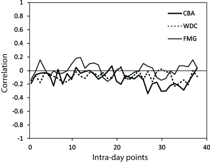
Figure 1: Correlation between cumulative volume $V^{(c)}_{i}=\sum_{j=1}^{i}V_{j}$ and the corresponding relative trading volume $V_{i}$ for CBA, WDC and FMG. Each correlation point is calculated for data sets obtained for the same time period $[t_{i},t_{i}+\Delta t]$ of available trading days.

Finally we note that some other tests suggested by Frei & Westray (2013) are also performed. The most important one being a test demonstrating a low correlation between cumulative ($\sum_{j=1}^{i}V_{j}$) and incremental volumes ($V_{i}$) within the same time period of a trading day $[t_{i},t_{i}+\Delta t]$ (i.e. day-to-day independence of $\sum_{j=1}^{i}V_{j}$ and $V_{i}$; see Frei & Westray (2013) for details). Figure 1 shows the corresponding intra-day correlations for CBA, WDC and FMG stocks, which are indeed reasonably low.

All results reported in this section strongly support the hypothesis that at least for the averaging interval of half a day or longer the stock volume dynamics can indeed be described as the standard gamma process: if the volume traded within the time period $[t_{i},t_{i}+\Delta t]$ is given by $V_{i}$, then we assume that it has the gamma distribution $\Gamma(\alpha,\theta)$, with mean $\alpha\theta$ and variance $\alpha\theta^{2}$, where $\alpha$ depends linearly on the averaging period $\Delta t$. Due to the independent increment property of the gamma process, volumes traded in disjoint time intervals of equal length are i.i.d.​ gamma variables.

4 Model for VWAP option pricing.

We now formally define a new model for the VWAP option pricing using a gamma process for volume dynamics. We work under the filtered probability space $(\Omega,\mathcal{F},\mathbb{F},\mathbb{Q})$. The filtration $\mathbb{F}=\{\mathcal{F}_{t}\}$ represents the flow of information available to market participants. In particular, it is the augmented filtration generated by a standard Brownian motion $W_{t}$ and a sequence of i.i.d.​ gamma variables $V_{1},\ldots,V_{N}\sim\Gamma(\alpha,\theta)$. For every $i=1,\ldots,N$, the gamma variable $V_{i}$ is $\mathcal{F}_{t_{i}}$-measurable where $t_{i}:=i\Delta t$ for some fixed time increment $\Delta t$. Note that the process $W_{t}$ and the random variables $\{V_{i}\}$ are assumed to be independent. For convenience we choose $W_{t}$ to be the Brownian motion under the risk-neutral pricing measure. So the measure $\mathbb{Q}$ is the product of the risk-neutral pricing measure and the real-world measure associated with $\{V_{i}\}$.

To summarise: the stock price process $S_{t}$ is given by the standard geometric Brownian motion d S_t = r S_t dt + σS_t dW_t, where $r$ is the risk-free interest rate and $\sigma$ is the volatility. Note that the discounted stock price $e^{-rt}S_{t}$ is a martingale under $\mathbb{Q}$.

The volumes traded $V_{t_{i}}$ traded during the time periods $[t_{i-1},t_{i}]$ (where $t_{i}=i\Delta t$) are directly modelled by the i.i.d.​ gamma variables, V_t_i := V_i ∼Γ(α,θ), with mean $\alpha\theta$ and variance $\alpha\theta^{2}$.

Now we can define the VWAP on a time interval $[0,T=N\Delta t]$ as

$$S^{\rm(VWAP)}=\frac{\sum^{N}_{i=1}S_{i}V_{i}}{\sum^{N}_{i=1}V_{i}}.$$ (1)

This paper will focus on the discrete-time formulation of VWAP VWAPd which is a weighted average of $N$ incremental trade volumes as opposed to a weighted integral over time. For completeness, the results for the continuous-time limit can be found in Appendix A. Note that we will consider the standard call and put VWAP options: