Strong-field tidal distortions of rotating black holes:
Formalism and results for circular, equatorial orbits

Abstract

Tidal coupling between members of a compact binary system can have an interesting and important influence on that binary’s dynamical inspiral. Tidal coupling also distorts the binary’s members, changing them (at lowest order) from spheres to ellipsoids. At least in the limit of fluid bodies and Newtonian gravity, there are simple connections between the geometry of the distorted ellipsoid and the impact of tides on the orbit’s evolution. In this paper, we develop tools for investigating tidal distortions of rapidly rotating black holes using techniques that are good for strong-field, fast-motion binary orbits. We use black hole perturbation theory, so our results assume extreme mass ratios. We develop tools to compute the distortion to a black hole’s curvature for any spin parameter, and for tidal fields arising from any bound orbit, in the frequency domain. We also develop tools to visualize the horizon’s distortion for black hole spin $a/M\leq\sqrt{3}/2$ (leaving the more complicated $a/M>\sqrt{3}/2$ case to a future analysis). We then study how a Kerr black hole’s event horizon is distorted by a small body in a circular, equatorial orbit. We find that the connection between the geometry of tidal distortion and the orbit’s evolution is not as simple as in the Newtonian limit.

I Introduction

I.1 Tidal coupling and binary inspiral

Tidal coupling in binary inspiral has been a topic of much recent interest. A great deal of attention has focused in particular on systems which contain neutron stars, where tides and their backreaction on the binary’s evolution may allow a new probe of the equation of state of neutron star matter rmsucf2009 ; hllr2010 ; dnv2012 . A great deal of work has been done to rigorously define the distortion of fluid stars dn2009 ; bp2009 , the coupling of the tidal distortion to the binary’s orbital energy and angular momentum bdgnr2010 , and most recently the importance of nonlinear fluid modes which can be sourced by tidal fields wab2013 ; vzh2014 .

Tidal coupling also plays a role in the evolution of binary black holes. Indeed, the influence of tidal coupling on binary black holes has been studied in some detail over the past two decades, but using rather different language: instead of “tidal coupling,” past literature typically discusses gravitational radiation “down the horizon.” This down-horizon radiation has a dual description in the tidal deformation of the black hole’s event horizon. A major purpose of this paper is to explore this dual description, examining quantitatively how a black hole is deformed by an orbiting companion.

Consider the down-horizon radiation picture first. The wave equation governing radiation produced in a black hole spacetime admits two solutions teuk73 ; tp74 , one describing outgoing radiation very far from the hole, and another describing radiation ingoing on the event horizon. Both solutions carry energy and angular momentum away from the binary, and drive (on average) a secular inspiral of the orbit. After suitable averaging, we require (for example) the orbital energy $E_{\rm orb}$ to evolve according to

$$\frac{dE_{\rm orb}}{dt}=-\left(\frac{dE}{dt}\right)^{\infty}-\left(\frac{dE}{dt}\right)^{\rm H}\;,$$ (1)

where $(dE/dt)^{\infty}$ describes energy carried far away by the waves, and $(dE/dt)^{\rm H}$ describes energy carried into the event horizon.

The down-horizon flux has an interesting property. When it is computed for a small body that is in a circular, equatorial orbit of a Kerr black hole with mass $M$ and spin parameter $a$, we find that

$$\left(\frac{dE}{dt}\right)^{\rm H}\propto\left(\Omega_{\rm orb}-\Omega_{\rm H}\right)\;,$$ (2)

where $\Omega_{\rm orb}=M^{1/2}/(r^{3/2}+aM^{1/2})$ is the orbital frequency, and $\Omega_{\rm H}=a/2Mr_{+}$ is the hole’s spin frequency (Ref. membrane , Sec VIID; see also synopsis in Sec. II.5). The radius $r_{+}=M+\sqrt{M^{2}-a^{2}}$ gives the location of the event horizon in Boyer-Lindquist coordinates. We assume that the orbit is prograde, so that the orbital angular momentum is parallel to the hole’s spin angular momentum.

When $\Omega_{\rm orb}>\Omega_{\rm H}$ (i.e., when the orbit rotates faster than the black hole spins), we have $(dE/dt)^{\rm H}>0$ — radiation carries energy into the horizon, taking it from the orbital energy. This is intuitively sensible, given that an event horizon generally acts as a sink for energy and matter. However, when $\Omega_{\rm orb}<\Omega_{\rm H}$ (the hole spins faster than the orbit’s rotation), we have $(dE/dt)^{\rm H}<0$. This means that the down-horizon component of the radiation augments the orbital energy — energy is transferred from the hole to the orbit. This is far more difficult to reconcile with the behavior of an event horizon.

One clue to understanding this behavior is that, when $\Omega_{\rm H}>\Omega_{\rm orb}$, the modes which contribute to the radiation are superradiant pt73 ; chandra . Consider a plane wave which propagates toward the black hole. A portion of the wave is absorbed by the black hole (changing its mass and spin), and a portion is scattered back out to large radius. A superradiant mode (see, for example, Sec. 98 of Ref. chandra ) is one in which the scattered wave has higher amplitude than the original ingoing wave. Some of the black hole’s spin angular momentum and rotational energy has been transferred to the radiation.

I.2 Tidally distorted strong gravity objects

Although the condition for superradiance is the same as the condition under which an orbit gains energy from the black hole, superradiance does not explain how energy is transferred from the hole to the orbit. A more satisfying picture of this can be built by invoking the dual picture of a tidal distortion. As originally shown by Hartle hartle73 ; hartle74 , an event horizon’s intrinsic curvature is distorted by a tidal perturbation. In analogy with tidal coupling in fluid systems, the tidally distorted horizon can gravitationally couple to the orbiting body, transfering energy and angular momentum from the black hole to the orbit.

Let us examine the fluid analogy in more detail for a moment. Consider in particular a moon that raises a tide on a fluid body, distorting its shape from spherical to a prolate ellipsoid. The tidal response will produce a bulge that tends to point at the moon. Due to the fluid’s viscosity, the bulging response will lag the driving tidal force. As a consequence, if the moon’s orbit is faster than the body’s spin, then the bulge will lag behind. The bulge will exert a torque on the orbit that tends to slow down the orbit; the orbit exerts a torque that tends to speed up the body’s spin. Conversely, if the spin is faster than the orbit, the bulge will lead the moon’s position, and the torque upon the orbit will tend to speed it up (and torque from the orbit tends to slow down the spin). In both cases, the bulge and moon exert torques on one another in such a way that the spin and orbit frequencies tend to be equalized. The action of this torque is such that energy is taken out of the moon’s orbit if the orbit frequency is larger than the spin frequency, and vice versa.

Since a black hole’s shape is changed by tidal forces in a manner similar to the change in shape of a fluid body, one can imagine that the horizon’s tidal bulge likewise exerts a torque on an orbit. Examining Eq. (2), we see that the sign of the “horizon flux” energy loss is exactly in accord with the tidal fluid analogy — energy is lost from the orbit if the orbital frequency exceeds the black hole’s spin frequency, and vice versa. Using the membrane paradigm membrane , one can assign a viscosity to the horizon, making the fluid analogy even more compelling.

However, as was first noted by Hartle hartle73 , the geometry of a black hole’s tidal bulge behaves in a rather counterintuitive manner. At least using a weak-field, slow spin analysis, the bulge leads the orbit when $\Omega_{\rm orb}>\Omega_{\rm H}$, and lags when $\Omega_{\rm orb}<\Omega_{\rm H}$. This is opposite to the geometry which the fluid analogy would lead us to expect. This is because an event horizon is a teleological object: Whether an event in spacetime is inside or outside a horizon depends on that event’s null future. At some moment in a given time slicing, an event horizon arranges itself in anticipation of the gravitational stresses it will be feeling in the future. This is closely related to the manner in which the event horizon of a spherical black hole expands outward when a spherical shell falls into it. See Ref. membrane , Sec. VI C 6 for further discussion.

Much of this background has been extensively discussed in past literature hartle73 ; hartle74 ; membrane ; tp08 ; dl2009 ; bp2009 ; pv2010 ; vpm11 . Recent work on this problem has examined in detail how one can quantify the tidal distortion of a black hole, demonstrating that the “gravitational Love numbers” which characterize the distortion of fluid bodies vanish for non-rotating black holes bp2009 , but that the geometry’s distortion can nonetheless be quantified assuming particularly useful coordinate systems dl2009 ; pv2010 and in a fully covariant manner vpm11 . Indeed, one can define “surficial Love numbers,” which quantify the distortion of a body’s surface, for Schwarzschild black holes lp14 . These techniques have been used to study horizon distortion in the Schwarzschild and slow spin limits, and for slow orbital velocities fl05 ; dl2009 ; vpm11 .

I.3 Our analysis: Strong-field, rapid spin tidal distortions

The primary goal of this paper is to develop tools to explore the distorted geometry of a black hole in a binary which are good for fast motion, strong field orbits. We use techniques originally developed by Hartle hartle74 to compute the Ricci scalar curvature $R_{\rm H}$ associated with the 2-surface of the distorted horizon; this is closely related to the intrinsic horizon metric developed in Ref. vpm11 . We will restrict our binaries to large mass ratios in order to use the tools of black hole perturbation theory. We also develop tools to embed the horizon in a 3-dimensional space in order to visualize the tidal distortions. In this paper, we restrict our embeddings to black hole spins $a/M\leq\sqrt{3}/2$. This is the largest spin at which the horizon can be embedded in a global Euclidean space; black holes with spins in the range $\sqrt{3}/2<a/M\leq 1$ must either be embedded in a space that is partially Euclidean, partially Lorentzian smarr , or be embedded in another space altogether frolov ; gibbons . Although no issue of principle prevents us for examining larger spins, it does not add very much to the physics we wish to study here, so we defer embeddings for $a/M>\sqrt{3}/2$ to a later paper.

A secondary goal of this paper is to investigate whether there is a simple connection between the geometry of the tidal bulge and the orbit’s evolution. In particular, we wish to see if the sign of $dE^{\rm H}/dt$, which is determined by $\Omega_{\rm orb}-\Omega_{\rm H}$, is connected to the bulge’s geometry relative to the orbit. This turns out to be somewhat tricky to investigate. The orbit and the horizon are at different locations, so we must map the orbit’s position onto the horizon. There is no unique way to do this, so the results depend at least in part on how we make the map. We present two maps from orbit to horizon. One, based on ingoing zero-angular momentum light rays, is useful for comparing with past literature. The other, based on the geometry of the horizon’s embedding and the orbit at an instant of constant ingoing time, is useful for describing our numerical data (at least for small spin). Another way to characterize the bulge geometry is to examine the relative phase of the bulge’s curvature to the tidal field which distorts the black hole. Both of these quantities are defined at $r=r_{+}$, so no mapping is necessary.

We find that, at the extremes, the response of a black hole to a perturbing tide follows Newtonian logic (modulo a swap of “lag” and “lead,” thanks to the horizon’s teleological nature). In particular, when $\Omega_{\rm orb}\gg\Omega_{\rm H}$ (so that $dE^{\rm H}/dt>0$), the bulge leads the orbit, no matter how we compare the bulge to the orbit. When $\Omega_{\rm orb}\ll\Omega_{\rm H}$ ($dE^{\rm H}/dt<0$), the bulge lags the orbit. However, relations between lag, lead, and $dE^{\rm H}/dt$ are not so clear cut when $\Omega_{\rm orb}\sim\Omega_{\rm H}$. Consider, in particular the case $\Omega_{\rm orb}=\Omega_{\rm H}$, for which $dE^{\rm H}/dt=0$. For Newtonian, fluid bodies, the tidal bulge points directly at the orbiting body in this case, with no exchange of torque between the body and the orbit. For black holes, we find no particular relation between the horizon’s bulge and the orbit’s position. The relation between tidal coupling and tidal distortion is far more complicated in black hole systems than it is for fluid bodies in Newtonian gravity — which is not especially surprising.

Soon after we submitted this paper and posted a preprint to the arXiv, Cabero and Krishnan posted an analysis of tidally deformed spinning black holes ck14 . Although their techniques and analysis differ quite a bit from ours (focusing on the Bowen-York by80 initial data set, and using the framework of isolated horizons), their results seem broadly consistent with ours. It may be useful in future work to explore this apparent consistency more closely, and to borrow some of the tools that they have developed for the systems that we analyze here.

I.4 Outline of this paper, units, and conventions

The remainder of this paper is organized as follows. Our formalism for computing the geometry of distorted Kerr black holes is given in Sec. II. We show how to compute the curvature of a tidally distorted black hole, and how to quantify the relation of the geometry of this distortion to the geometry of the orbit which produces the tidal field. We also discuss how to compute $dE^{\rm H}/dt$, demonstrating that the information which determines this down-horizon flux is identical to the information which determines the geometry of the distorted event horizon.

Sections III and IV present results for Schwarzschild and Kerr, respectively. In both sections, we first look at the black hole’s curvature in a slow motion, slow spin expansion (slow motion only for Schwarzschild). This allows us to develop analytic expressions for the curvature, which are useful for comparing to the fast motion, rapid spin numerical results that we then compute. We visualize tidally distorted black holes by embedding their horizons in a 3-dimensional space. This provides a useful way to see how tides change the shape of a black hole. In Sec. V, we examine in some detail whether there is a simple connection between a black hole’s tidally distorted geometry and the coupling between the hole and the orbit. In short, the answer we find is “no” — Newtonian, fluid intuition breaks down for black holes and strong-field orbits.

Concluding discussion is given in Sec. VI, followed by certain lengthy technical details which we relegate to appendices. Appendix A describes in detail how to compute $\bar{\eth}$, a Newman-Penrose operator which lowers the spin-weight of quantities needed for our analysis. Appendix B describes how to embed a distorted black hole’s event horizon in a 3-dimensional Euclidean space. As mentioned above, one cannot embed black holes with $a/M>\sqrt{3}/2$ in Euclidean space, but must use a either a mixed Euclidean/Lorentzian space smarr , or something altogether different frolov ; gibbons . We will examine the range $a/M>\sqrt{3}/2$ in a later paper. Appendix C computes, to leading order in spin, the spheroidal harmonics which are used as basis functions in black hole perturbation theory. This is needed for the slow-spin expansions we present in Sec. IV. Finally, Appendix D summarizes certain changes in notation that we have introduced versus previous papers that use black hole perturbation theory. These changes synchronize our notation with that used in the literature from which we have recently adopted our core numerical method ft04 ; ft05 .

All of our calculations are done in the background of a Kerr black hole. Two coordinate systems, described in detail in Ref. poisson , are particularly useful for us. The Boyer-Lindquist coordinates ($t,r,\theta,\phi$) yield the line element

$$ds^{2} = -\left(1-\frac{2Mr}{\Sigma}\right)dt^{2}-\frac{4Mar\sin^{2}\theta}{\Sigma}dt\,d\phi+\frac{\Sigma}{\Delta}dr^{2}$$ (3)

$$+ \!\!\Sigma\,d\theta^{2}+\frac{(r^{2}+a^{2})^{2}-a^{2}\Delta\sin^{2}\theta}{\Sigma}\sin^{2}\theta\,d\phi^{2}\;,$$

where

$$\Delta=r^{2}-2Mr+a^{2}\;,\qquad\Sigma=r^{2}+a^{2}\cos^{2}\theta\;.$$ (4)

The function $\Delta$ has two roots, $r_{\pm}=M\pm\sqrt{M^{2}-a^{2}}$; $r_{+}$ is the location of the event horizon. We will also often find it useful to use ingoing coordinates $(v,r^{\prime},\theta,\psi)$, related to the Boyer-Lindquist coordinates by poisson

$$dv = dt+\frac{(r^{2}+a^{2})}{\Delta}\,dr\;,$$ (5)

$$d\psi = d\phi+\frac{a}{\Delta}\,dr\;.$$ (6)

$$dr^{\prime} = dr\;,$$ (7)

These coordinates are well-behaved on the event horizon, and so are useful tools for describing fields that fall into the hole. Although the relation between $r$ and $r^{\prime}$ is trivial, it can be useful to distinguish the two as a bookkeeping device when transforming between the two coordinate systems. When there is no ambiguity, we will drop the prime on the ingoing radial coordinate. The Kerr metric in ingoing coordinates is given by

$$ds^{2} = -\left(1-\frac{2Mr^{\prime}}{\Sigma}\right)dv^{2}+2dv\,dr^{\prime}-2a\sin^{2}\theta\,dr^{\prime}\,d\psi$$

$$- \!\!\frac{4Mar^{\prime}\sin^{2}\theta}{\Sigma}dv\,d\psi$$

$$+ \!\!\Sigma\,d\theta^{2}+\frac{[(r^{\prime})^{2}+a^{2}]^{2}-a^{2}\Delta\sin^{2}\theta}{\Sigma}\sin^{2}\theta\,d\psi^{2}\;.$$

The quantities $\Sigma$ and $\Delta$ here are exactly as in Eq. (4), but with $r\to r^{\prime}$.

It is not difficult to integrate up Eqs. (5) and (6) to find

$$v=t+r^{*}\;,\qquad\psi=\phi+\bar{r}\;,$$ (9)

where poisson

$$r^{*} = r+\frac{Mr_{+}}{\sqrt{M^{2}-a^{2}}}\ln\left(\frac{r}{r_{+}}-1\right)$$ (10)

$$\qquad-\frac{Mr_{-}}{\sqrt{M^{2}-a^{2}}}\ln\left(\frac{r}{r_{-}}-1\right)\;,$$

$$\bar{r} = \frac{a}{2\sqrt{M^{2}-a^{2}}}\ln\left(\frac{r-r_{+}}{r-r_{-}}\right)\;.$$ (11)

Notice that $\psi=\phi$ when $a=0$.

For $r=r_{+}+\delta r$, $\delta r\ll M$,

$$\bar{r}-\Omega_{\rm H}r^{*}=K(a)+O(\delta r)\;,$$ (12)

where

$$K(a) = \frac{a}{2M(Mr_{+}-a^{2})}\biggl{\{}a^{2}-Mr_{+}$$

$$+ 2M^{2}{\rm arctanh}\left(\sqrt{1-a^{2}/M^{2}}\right)$$

$$+ M\sqrt{M^{2}-a^{2}}\ln\left[\frac{a^{2}}{4(M^{2}-a^{2})}\right]\biggr{\}}$$

$$= -\frac{a}{2M}+\left[1-2\ln\left(\frac{a}{2M}\right)\right]\left(\frac{a}{2M}\right)^{3}+O(a^{5})\;.$$

This means that, near the horizon, the combination $\bar{r}-\Omega_{\rm H}r^{*}$ cancels out the logarithms in both $r^{*}$ and $\bar{r}$, trending to a constant $K(a)$ that depends only on spin. The quantity $K(a)$ plays an important role in setting the phase of tidal fields on the event horizon.

II Formalism

In this section, we develop the formalism we use to study the geometry of deformed event horizons. The details of this calculation are presented in Sec. II.1. Two pieces of this calculation are sufficiently involved that we present them separately. First, in Sec. II.2, we give an overview of how one solves the radial perturbation equation to find the amplitude that sets the magnitude of the tidal distortion. This material has been discussed at great length in many other papers, so we present just enough detail to illustrate what is needed for our analysis. We include in our discussion the static limit, mode frequency $\omega=0$. Since static modes do not carry energy or angular momentum, they have been neglected in almost all previous analyses. However, these modes affect the shape of a black hole, so they must be included here. Second, in Sec. II.3 we provide detailed discussion of the angular operator $\bar{\eth}\bar{\eth}$ and its action upon the spin-weighted spheroidal harmonic.

Section II.4 describes how we characterize the bulge in the event horizon which is raised by the orbiting body’s tide. The bulge is a simple consequence of the geometry, but this discussion deserves separate treatment in order to properly discuss certain choices and conventions we must make. We conclude this section by briefly reviewing down-horizon fluxes in Sec. II.5. Although this discussion is tangential to our main focus in this paper, we do this to explicitly show that the deformed geometry and the down-horizon flux are just different ways of presenting the same information about the orbiting body’s perturbation to the black hole.

II.1 The geometry of an event horizon

We will characterize the geometry of distorted black holes using the Ricci scalar curvature $R_{\rm H}$ associated with their event horizon’s 2-surface. The scalar curvature of an undistorted Kerr black hole is given by smarr

$$R_{\rm H}=R^{(0)}_{\rm H}=\frac{2}{r_{+}^{2}}\frac{(1+a^{2}/r_{+}^{2})(1-3a^{2}\cos^{2}\theta/r_{+}^{2})}{(1+a^{2}\cos^{2}\theta/r_{+}^{2})^{3}}\;.$$ (14)

For $a=0$, $R^{(0)}_{\rm H}=2/r_{+}^{2}$, the standard result for a sphere of radius $r_{+}$. For $a/M\geq\sqrt{3}/2$, $R^{(0)}_{\rm H}$ changes sign near the poles. This introduces important and interesting complications to how we represent the tidal distortions of a rapidly rotating black hole’s horizon.

To first order in the mass ratio, tidal distortions leave the horizon at the coordinate $r=r_{+}$, but change the scalar curvature on that surface (at least in all “horizon-locking gauges” vpm11 , which we implicitly use in our analysis). Using the Newman-Penrose formalism np62 , Hartle hartle74 shows that the perturbation $R^{(1)}_{\rm H}$ to the curvature is simply related to the perturbing tidal field $\psi_{0}$:

$$R^{(1)}_{\rm H} = -4\,{\rm Im}\sum_{lmkn}\frac{\bar{\eth}\bar{\eth}\psi^{\rm HH}_{0,lmkn}}{p_{mkn}(ip_{mkn}+2\epsilon)}$$ (15)

$$\equiv \sum_{lmkn}R^{(1)}_{{\rm H},lmkn}\;,$$

with all quantities evaluated at $r=r_{+}$. The quantity $\psi^{\rm HH}_{0,lmkn}$ is a term in a multipolar and harmonic expansion of the Newman-Penrose curvature scalar $\psi_{0}$, computed using the Hawking-Hartle tetrad hh72 :

$$\psi^{\rm HH}_{0} \equiv -C_{\alpha\beta\gamma\delta}(l^{\alpha})^{\rm HH}(m^{\beta})^{\rm HH}(l^{\gamma})^{\rm HH}(m^{\delta})^{\rm HH}$$ (16)

$$= \sum_{lmkn}\psi_{0,lmkn}^{\rm HH}\;.$$

The tensor $C_{\alpha\beta\gamma\delta}$ is the Weyl curvature, and the vectors $(l^{\alpha})^{\rm HH}$ and $(m^{\alpha})^{\rm HH}$ are Newman-Penrose tetrad legs in the Hawking-Hartle representation. See Appendix A for detailed discussion of this tetrad and related quantities.

We assume that $\psi_{0}$ arises from an object in a bound orbit of the Kerr black hole. This object’s motion can be described using the three fundamental frequencies associated with such orbits: an axial frequency $\Omega_{\phi}$, a polar frequency $\Omega_{\theta}$, and a radial frequency $\Omega_{r}$. The indices $m$, $k$, and $n$ label harmonics of these frequencies:

$$\omega_{mkn}=m\Omega_{\phi}+k\Omega_{\theta}+n\Omega_{r}\;.$$ (17)

The index $l$ labels a spheroidal harmonic mode, and is discussed in more detail below. The remaining quantities appearing in Eq. (15) are the wavenumber for ingoing radiation

$$p_{mkn}=\omega_{mkn}-m\Omega_{\rm H}\;,$$ (18)

and

$$\epsilon=\frac{\sqrt{M^{2}-a^{2}}}{4Mr_{+}}\equiv\frac{\kappa}{2}\;.$$ (19)

The quantity $\kappa$ is the Kerr surface gravity. We will find this interpretation of $\epsilon$ to be useful when discussing the geometry of the horizon’s tidal distortion. We discuss the operator $\bar{\eth}\bar{\eth}$ in detail in Sec. II.3. For now, note that it involves derivatives with respect to $\theta$.

The calculation of $R^{(1)}_{\rm H}$ involves several computations that use the Newman-Penrose derivative operator $D\equiv l^{\alpha}\partial_{\alpha}$. Using the Hawking-Hartle form of $l^{\alpha}$ and ingoing Kerr coordinates (see Appendix A), we find that

$$D\to\frac{\partial}{\partial v}+\Omega_{\rm H}\frac{\partial}{\partial\psi}$$ (20)

as $r\to r_{+}$. The fields to which we apply this operator have the form $e^{i(m\psi-\omega_{mkn}v)}$ near the horizon, so

$$D{\cal F}=i(m\Omega_{\rm H}-\omega_{mkn}){\cal F}=-ip_{mkn}{\cal F}$$ (21)

for all relevant fields ${\cal F}$. Hartle choses a time coordinate $t$ such that $D\equiv\partial/\partial t$ near the horizon, effectively working in a frame that corotates with the black hole. As a consequence, his Eq. (2.21) [equivalent to our Eq. (15)] has $\omega$ in place of $p$. Hartle’s (2.21) also corresponds to a single Fourier mode, and so is not summed over indices.

The Hawking-Hartle tetrad is used in Eq. (16) because it is well behaved on the black hole’s event horizon hh72 . In many discussions of black hole perturbation theory based on the Teukolsky equation, we instead use the Kinnersley tetrad, which is well designed to describe distant radiation teuk73 ; kinnersley . The Kinnersley tetrad is described explicitly in Appendix A. The relation between $\psi_{0}$ in these two tetrads is [cf. Ref. tp74 , Eq. (4.43)]

$$\psi_{0}^{\rm HH}=\frac{\Delta^{2}}{4(r^{2}+a^{2})^{2}}\psi_{0}^{\rm K}\;.$$ (22)

Further, we know that $\psi_{0}^{\rm K}$ on the horizon can be written tp74

$$\psi_{0,lmkn}^{\rm K}=\frac{W^{\rm H}_{lmkn}\,{{}_{+2}S}_{lm}(\theta;a\omega_{mkn})}{\Delta^{2}}e^{i(m\phi-\omega_{mkn}t-p_{mkn}r^{*})}\;.$$ (23)

We have introduced $W^{\rm H}_{lmkn}$, a complex amplitude which we will discuss in more detail below, as well as the spheroidal harmonic of spin-weight $+2$, ${{}_{+2}S}_{lm}(\theta;a\omega_{mkn})$. Spheroidal harmonics are often used in black hole perturbation theory, since the equations governing a field of spin-weight $s$ in a black hole spacetime separate when these harmonics are used as a basis for the $\theta$ dependence. In the limit $a\omega_{mkn}\to 0$, they reduce to the spin-weighted spherical harmonics:

$${{}_{s}S}_{lm}(\theta;a\omega_{mkn})\to{{}_{s}Y}_{lm}(\theta)\quad\mbox{as}\quad a\omega_{mkn}\to 0\;.$$ (24)

${{}_{s}Y}_{lm}(\theta)$ denotes the spherical harmonic without the axial dependence: ${{}_{s}}Y_{lm}(\theta,\phi)={{}_{s}}Y_{lm}(\theta)e^{im\phi}$. In what follows, we will abbreviate:

$${{}_{+2}S}_{lm}(\theta;a\omega_{mkn})\equiv S^{+}_{lmkn}(\theta)\;.$$ (25)

We will likewise write the spin-weight $-2$ spheroidal harmonic as $S^{-}_{lmkn}(\theta)$.

Combining Eqs. (22) and (23), we find

$$\psi^{\rm HH}_{0,lmkn}=\frac{W^{\rm H}_{lmkn}S^{+}_{lmkn}(\theta)}{4(r^{2}+a^{2})^{2}}\,e^{i(m\phi-\omega_{mkn}t-p_{mkn}r^{*})}\;.$$ (26)

Using Eqs. (9) and (18), we can rewrite the phase factor using coordinates that are well-behaved on the horizon:

$$m\phi-\omega_{mkn}t-p_{mkn}r^{*}\! = m(\psi-\bar{r})-\omega_{mkn}(v-r^{*})$$

$$-(\omega_{mkn}-m\Omega_{\rm H})r^{*}$$

$$= m\psi-\omega_{mkn}v-m(\bar{r}-\Omega_{\rm H}r^{*})\;.$$

Taking the limit $r\to r_{+}$ and using Eq. (12), we find

$$\psi^{\rm HH}_{0,lmkn}=\frac{W^{\rm H}_{lmkn}S^{+}_{lmkn}(\theta)}{16M^{2}r_{+}^{2}}e^{i\Phi_{mkn}(v,\psi)}\;,$$ (28)

where

$$\Phi_{mkn}(v,\psi)=m\psi-\omega_{mkn}v-mK(a)\;,$$ (29)

with $K(a)$ defined in Eq. (LABEL:eq:K_of_a). We finally find

$$R^{(1)}_{{\rm H},lmkn}=-{\rm Im}\left[\frac{W^{\rm H}_{lmkn}e^{i\Phi_{mkn}(v,\psi)}\bar{\eth}\bar{\eth}S^{+}_{lmkn}(\theta)}{4M^{2}r_{+}^{2}p_{mkn}(ip_{mkn}+2\epsilon)}\right]\;.$$

(30)

We will use a Teukolsky equation solver h2000 ; dh2006 ; thd_inprep which computes the curvature scalar $\psi_{4}$ rather than $\psi_{0}$. Although $\psi_{4}$ is usually used to study radiation far from the black hole, one can construct $\psi_{0}$ from it using the Starobinsky-Churilov identities tp74 ; sc73 . In the limit $r\to r_{+}$,

$$\psi_{4} = \frac{\Delta^{2}}{(r-ia\cos\theta)^{4}}\sum_{lmkn}Z^{\rm H}_{lmkn}S^{-}_{lmkn}(\theta)$$ (31)

$$\qquad\qquad\times\,e^{i(m\phi-\omega_{mkn}t-p_{mkn}r^{*})}\;.$$

We briefly summarize how we compute $Z^{\rm H}_{lmkn}$ in Sec. II.2. Using the Starobinsky-Churilov identities, we find that $Z^{\rm H}_{lmkn}$ and $W^{\rm H}_{lmkn}$ are related by

$$W^{\rm H}_{lmkn}=\beta_{lmkn}Z^{\rm H}_{lmkn}\;,$$ (32)

where

$$\beta_{lmkn}=\frac{64(2Mr_{+})^{4}p_{mkn}(p_{mkn}^{2}+4\epsilon^{2})(p_{mkn}+4i\epsilon)}{c_{lmkn}}\;,$$ (33)

and where the complex number $c_{lmkn}$ is given by

$$|c_{lmkn}|^{2} = \left\{\left[(\lambda+2)^{2}+4ma\omega_{mkn}-4a^{2}\omega_{mkn}^{2}\right]\right.$$ (34)

$$\left.\qquad\times\left(\lambda^{2}+36ma\omega_{mkn}-36a^{2}\omega_{mkn}^{2}\right)\right.$$

$$\left.\qquad+\,(2\lambda+3)(96a^{2}\omega_{mkn}^{2}-48ma\omega_{mkn})\right\}$$

$$+144\omega_{mkn}^{2}(M^{2}-a^{2})\;,$$

$${\rm Im}\,c_{lmkn} = 12M\omega_{mkn}\;,$$ (35)

$${\rm Re}\,c_{lmkn} = +\sqrt{|c_{lmkn}|^{2}-144M^{2}\omega_{mkn}^{2}}\;.$$ (36)

The real number $\lambda$ appearing here is

$$\lambda={\cal E}_{lmkn}-2am\omega_{mkn}+a^{2}\omega_{mkn}^{2}-2\;,$$ (37)

with ${\cal E}_{lmkn}$ the eigenvalue of $S^{-}_{lmkn}(\theta)$. In the limit $a\omega_{mkn}\to 0$, ${\cal E}_{lmkn}\to l(l+1)$. For our later weak-field expansion, it will be useful to have $\lambda$ as an expansion in $a\omega_{mkn}$. See Appendix C for discussion of this.

Using these results, we can write the tidal distortion of the horizon’s curvature as

$$R^{(1)}_{{\rm H},lmkn} = -{\rm Im}\left[\frac{\beta_{lmkn}Z^{\rm H}_{lmkn}e^{i\Phi_{mkn}(v,\psi)}\bar{\eth}\bar{\eth}S^{+}_{lmkn}(\theta)}{4M^{2}r_{+}^{2}p_{mkn}(ip_{mkn}+2\epsilon)}\right]$$

$$\equiv {\rm Im}\left[{\cal C}_{lmkn}Z^{\rm H}_{lmkn}e^{i\Phi_{mkn}(v,\psi)}\bar{\eth}\bar{\eth}S^{+}_{lmkn}(\theta)\right]\;,$$

where

$${\cal C}_{lmkn}=256M^{2}r_{+}^{2}c_{lmkn}^{-1}(p_{mkn}+4i\epsilon)(ip_{mkn}-2\epsilon)\;.$$ (39)

Equation (LABEL:eq:gauss_kerr) is the workhorse of our analysis. We use a slightly modified version of the code described in Refs. h2000 ; dh2006 ; thd_inprep to compute the complex numbers $Z^{\rm H}_{lmkn}$ and the angular function $\bar{\eth}\bar{\eth}S^{+}_{lmkn}$. We briefly describe these calculations in the next two subsections.

II.2 Computing $Z^{\rm H}_{lmkn}$

Techniques for computing the amplitude $Z^{\rm H}_{lmkn}$ have been discussed in great detail in other papers, so our discussion here will be very brief; our analysis follows that given in Ref. dh2006 . The major change versus previous works is that we need the solution for static modes ($\omega=0$). Our goal here is to present enough detail to see how earlier studies can be modified fairly simply to include these modes. It is worth noting that we have changed notation from that used in previous papers by our group in order to more closely follow the notation of Fujita and Tagoshi ft04 ; ft05 . Appendix D summarizes these changes.

The complex number $Z^{\rm H}_{lmkn}$ is the amplitude of solutions to the Teukolsky equation for spin-weight $s=-2$, so we begin there:

$$\Delta^{2}\frac{d}{dr}\left(\frac{dR_{lm\omega}}{dr}\right)-V_{lm}(r)R_{lm\omega}={\cal T}_{lm\omega}(r)\;.$$ (40)

This is the frequency-domain version of this equation, following the introduction of a modal and harmonic decomposition which separates the original time-domain equation; see teuk73 for further details. The potential $V_{lm}$ is discussed in Sec. IIIA of Ref. dh2006 ; the source term ${\cal T}_{lm\omega}$ is discussed in Sec. IIIB of that paper.

Equation (40) has two homogeneous solutions relevant to our analysis: The “in” solution is purely ingoing on the horizon, but is a mixture of ingoing and outgoing at future null infinity; the “up” solution is purely outgoing at future null infinity, but is a mixture of ingoing and outgoing on the horizon. We discuss these solutions in more detail below. For now, it is enough that these solutions allow us to build a Green’s function poisson93 ,

$$G(r|r^{\prime}) = \frac{1}{{\cal W}}R^{\rm up}_{lm\omega}(r)R^{\rm in}_{lm\omega}(r^{\prime})\;,\quad r^{\prime}<r\;,$$ (41)

$$= \frac{1}{{\cal W}}R^{\rm in}_{lm\omega}(r)R^{\rm up}_{lm\omega}(r^{\prime})\;,\quad r^{\prime}>r\;,$$

where

$${\cal W}=\frac{1}{\Delta}\left[R^{\rm in}_{lm\omega}\frac{dR^{\rm up}_{lm\omega}}{dr}-R^{\rm up}_{lm\omega}\frac{dR^{\rm in}_{lm\omega}}{dr}\right]$$ (42)

is the equation’s Wronskian. This is then integrated against the source to build the general inhomogeneous solution:

$$R_{lm\omega}(r) = \int_{r_{+}}^{\infty}G(r|r^{\prime}){\cal T}_{lm\omega}(r^{\prime})dr^{\prime}$$

$$\equiv Z^{\rm in}_{lm\omega}(r)R^{\rm up}_{lm\omega}(r)+Z^{\rm up}_{lm\omega}(r)R^{\rm in}_{lm\omega}(r)\;.$$

We have defined

$$Z^{\rm in}_{lm\omega}(r) = \frac{1}{\cal W}\int_{r_{+}}^{r}\frac{R^{\rm in}_{lm\omega}(r^{\prime}){\cal T}_{lm\omega}(r^{\prime})}{\Delta(r^{\prime})^{2}}dr^{\prime}\;,$$ (44)

$$Z^{\rm up}_{lm\omega}(r) = \frac{1}{\cal W}\int_{r}^{\infty}\frac{R^{\rm up}_{lm\omega}(r^{\prime}){\cal T}_{lm\omega}(r^{\prime})}{\Delta(r^{\prime})^{2}}dr^{\prime}\;.$$ (45)

A key property of ${\cal T}_{lm\omega}$ is that it is the sum of three terms, one proportional to $\delta[r-r_{\rm orb}(t)]$, one proportional to $\delta^{\prime}[r-r_{\rm orb}(t)]$, and one proportional to $\delta^{\prime\prime}[r-r_{\rm orb}(t)]$ (where ^′ denotes $d/dr$). Putting this into Eqs. (44) and (45), we find that

$$Z^{\star}_{lm\omega}(r) = \frac{1}{\cal W}\Biggl{\{}{\cal I}^{0}_{lm\omega}\left[R^{\star}_{lm\omega}(r)\right]+{\cal I}^{1}_{lm\omega}\left[\frac{dR^{\star}_{lm\omega}}{dr}\biggr{|}_{r}\right]$$ (46)

$$+{\cal I}^{2}_{lm\omega}\left[\frac{d^{2}R^{\star}_{lm\omega}}{dr^{2}}\biggr{|}_{r}\right]\Biggr{\}}\;,$$

(where $\star$ can stand for “up” or “in”). The factors ${\cal I}^{0,1,2}_{lm\omega}$ are operators which act on $R^{\star}_{lm\omega}$ and its derivatives. These operators integrate over the $r$ and $\theta$ motion of the orbiting body.

In this analysis, we are concerned with the solution of the perturbation equation on the event horizon, so we want $R_{lm\omega}$ as $r\to r_{+}$. In this limit, $Z^{\rm in}_{lm\omega}=0$. We define

$$Z^{\rm H}_{lm\omega}\equiv Z^{\rm up}_{lm\omega}(r_{+})\;.$$ (47)

For a source term corresponding to a small body in a bound Kerr orbit, we find that Eq. (46) has the form

$$Z^{\rm H}_{lm\omega}=\sum_{kn}Z^{\rm H}_{lmkn}\delta(\omega-\omega_{mkn})\;.$$ (48)

It is then not difficult to read off $Z^{\rm H}_{lmkn}$. See Ref. dh2006 for detailed discussion of how to evaluate Eq. (46) and read off these amplitudes.

Key to computing $Z^{\rm H}_{lmkn}$ is computing the homogeneous solutions $R^{\rm up}_{lm\omega}(r)$, $R^{\rm in}_{lm\omega}(r)$, and their derivatives. Our methods for doing this depend on whether $\omega_{mkn}$ is zero or not.

II.2.1 $\omega_{mkn}\neq 0$

The homogeneous solutions for $\omega_{mkn}\neq 0$ have been amply discussed in the literature; our analysis is based on that of Ref. dh2006 . In brief, the two homogeneous solutions of Eq. (40) have the following asymptotic behavior:

$$R^{\rm in}_{lm\omega}(r\to r_{+}) = B^{\rm trans}_{lm\omega}\Delta^{2}e^{-ipr^{*}}\;,$$ (49)

$$R^{\rm in}_{lm\omega}(r\to\infty) = B^{\rm ref}_{lm\omega}r^{3}e^{i\omega r^{*}}+\frac{B^{\rm inc}_{lm\omega}}{r}e^{-i\omega r^{*}}\;;$$

$$R^{\rm up}_{lm\omega}(r\to r_{+}) = C^{\rm up}_{lm\omega}e^{ipr^{*}}+C^{\rm ref}_{lm\omega}\Delta^{2}e^{-ipr^{*}}\;,$$

$$R^{\rm up}_{lm\omega}(r\to\infty) = C^{\rm trans}_{lm\omega}r^{3}e^{i\omega r^{*}}\;.$$ (52)

These asymptotic solutions yield the Wronskian:

$${\cal W}=2i\omega B^{\rm inc}_{lm\omega}C^{\rm trans}_{lm\omega}\;.$$ (53)

An effective algorithm for computing all of the quantities which we need is described by Fujita and Tagoshi st03 ; ft04 ; ft05 . It is based on expanding the solution in a basis of hypergeometric and Coulomb wave functions, with the coefficients of the expansion determined by solving a recurrence relation; see Secs. 4.2 – 4.4 of Ref. st03 for detailed discussion. We use a code based on these methods thd_inprep for all of our $\omega_{mkn}\neq 0$ calculations; the analytic limits we present in Secs. III.1 and IV.1 are also based on these methods.

II.2.2 $\omega_{mkn}=0$

Static modes have been neglected in much past work. They do not carry any energy or angular momentum, and so are not important for many applications. These modes do play a role in setting the shape of the distorted event horizon, however, and must be included here.

It turns out that homogeneous solutions for $\omega_{mkn}=0$ are available as surprisingly simple closed form expressions. Teukolsky’s Ph.D. thesis teukphd presents two solutions that satisfy appropriate boundary conditions. Defining

$$x=\frac{r-r_{+}}{r_{+}-r_{-}}\;,\quad\gamma=\frac{iam}{r_{+}-r_{-}}\;,$$ (54)

the two solutions of the radial Teukolsky equation for $s=-2$ are

$$R^{\rm in}_{lm0}(r) = (r_{+}-r_{-})^{4}x^{2}(1+x)^{2}\left(\frac{x}{1+x}\right)^{\gamma}\,\times$$ (55)

$${}_{2}F_{1}(2-l,l+3;3+2\gamma,-x)\;,$$

$$R^{\rm up}_{lm0}(r) = (r_{+}-r_{-})^{(1-l)}x^{(1-l)}(1+1/x)^{(2-\gamma)}\,\times$$

$${}_{2}F_{1}(l+3,l+1-2\gamma;2l+2,-1/x)\;.$$

In these equations, ${}_{2}F_{1}(a,b;c,x)$ is the hypergeometric function. These solutions satisfy regularity conditions at infinity and on the horizon: $R^{\rm in}_{lm0}(r\to r_{+})\propto\Delta^{2}$, and $R^{\rm up}_{lm0}(r\to\infty)\propto 1/r^{l-1}$ teukphd . We have introduced powers of $r_{+}-r_{-}$ to insure that we have the correct asymptotic behavior in $r$, rather than in the dimensionless variable $x$. The Wronskian corresponding to these solutions is

$${\cal W}=-\frac{(2l+1)!}{(l+2)!}\frac{\Gamma(3+2\gamma)}{\Gamma(l+1+2\gamma)}(r_{+}-r_{-})^{(2-l)}\;.$$ (57)

Using Eqs. (55), (LABEL:eq:Rup_omega0), and (57), it is simple to adapt existing codes to compute $Z^{\rm H}_{lmkn}$ for $\omega_{mkn}=0$.

The results we present in Secs. III and IV will focus on circular, equatorial orbits, for which $k=n=0$. The zero-frequency modes in this limit have $m=0$, for which $\gamma=0$. The Wronskian simplifies further:

$${\cal W}_{(m=0)}=-\frac{2(2l+1)!}{l!(l+2)!}(r_{+}-r_{-})^{(2-l)}\;.$$ (58)

For generic orbit geometries, there will exist cases that have $\omega_{mkn}=0$ with $m\neq 0$, akin to the “resonant” orbits studied at length in Refs. fh12 ; fhr14 . We defer discussion of this possibility to a later analysis which will go beyond circular and equatorial orbits.

II.3 The operator $\bar{\eth}\bar{\eth}$

The operator $\bar{\eth}$, when acting on a quantity $\eta$ of spin-weight $s$, takes the following form:

$$\bar{\eth}\eta=\left[\bar{\delta}-(\alpha-\bar{\beta})\right]\eta\;;$$ (59)

$\bar{\eth}\eta$ is then a quantity of spin-weight $s-1$. The quantities $\alpha$ and $\beta$ are both Newman-Penrose spin coefficients, and $\bar{\delta}$ is a Newman-Penrose derivative operator. These quantities are all related to the tetrad legs ${\bf m}$, $\bar{\bf m}$:

$$\bar{\delta} = \bar{m}^{\mu}\partial_{\mu}\;,$$ (60)

$$\alpha-\bar{\beta} = \frac{1}{2}\bar{m}^{\nu}\left(\bar{m}^{\mu}\nabla_{\nu}m_{\mu}-m^{\mu}\nabla_{\nu}\bar{m}_{\mu}\right)\;.$$ (61)

We do this calculation using the Hawking-Hartle tetrad; details are given in Appendix A. The result for general black hole spin $a$ is

$$\bar{\eth}\eta = \frac{1}{\sqrt{2}(r_{+}-ia\cos\theta)}\Biggl{(}L^{s}_{-}-am\Omega_{\rm H}\sin\theta$$ (62)

$$\qquad\qquad\qquad\quad-\frac{isa\sin\theta}{r_{+}-ia\cos\theta}\Biggr{)}\eta\;.$$

The operator $L^{s}_{-}$ lowers the spin-weight of the spherical harmonics by 1:

$$L^{s}_{-}{{}_{s}Y}_{lm} = \left(\partial_{\theta}+s\cot\theta+m\csc\theta\right){{}_{s}Y}_{lm}$$ (63)

$$= \sqrt{(l+s)(l-s+1)}{{}_{s-1}Y}_{lm}\;.$$

In a few places, we will need to evaluate $L^{s}_{-}\left[\cos\theta\eta\right]$ and $L^{s}_{-}\left[\sin\theta\eta\right]$. This requires that we rewrite $\cos\theta$ and $\sin\theta$ in a form that properly indicates their spin weight. We treat $\cos\theta$ as spin-weight zero, writing

$$\cos\theta=\sqrt{\frac{4\pi}{3}}\,{{}_{0}}Y_{10}\;.$$ (64)

Likewise, we treat $\sin\theta$ as spin-weight $-1$, writing

$$\sin\theta=-\sqrt{\frac{8\pi}{3}}\,{{}_{-1}}Y_{10}\;.$$ (65)

This accounts for the fact that $\sin\theta$ always appears in our calculation inside operators that lower spin-weight.

With this, we find the following identities:

$$L^{s}_{-}\left[\cos\theta\eta\right] = \sqrt{\frac{4\pi}{3}}L^{s}_{-}\left[{{}_{0}}Y_{10}\,\eta\right]$$ (66)

$$= \sqrt{\frac{4\pi}{3}}\left({{}_{0}}Y_{10}\,L^{s}_{-}\eta+\eta\,L^{s}_{-}\,{{}_{0}}Y_{10}\right)$$

$$= \sqrt{\frac{4\pi}{3}}\left({{}_{0}}Y_{10}\,L^{s}_{-}\eta+\eta\,\sqrt{2}\,{{}_{-1}}Y_{10}\right)$$

$$= \cos\theta\,L^{s}_{-}\eta-\sin\theta\eta\;;$$

$$L^{s}_{-}\left[\sin\theta\eta\right] = -\sqrt{\frac{8\pi}{3}}L^{s}_{-}\left[{}_{-1}Y_{10}\eta\right]$$ (67)

$$= -\sqrt{\frac{8\pi}{3}}\left({}_{-1}Y_{10}\,L^{s}_{-}\eta+\eta\,L^{s}_{-}\,{{}_{-1}}Y_{10}\right)$$

$$= -\sqrt{\frac{8\pi}{3}}\,{{}_{-1}Y}_{10}L^{s}_{-}\,\eta$$

$$= \sin\theta\,L^{s}_{-}\eta\;.$$

We used the fact that $L^{s}_{-}$ applied to ${{}_{-1}Y}_{10}$ yields zero.

Using these results, it follows that

$$L^{s}_{-}\left(1-\frac{ia\cos\theta}{r_{+}}\right)^{-s}\eta = \left(1-\frac{ia\cos\theta}{r_{+}}\right)^{-s}$$

$$\!\!\!\!\!\!\!\!\!\!\!\!\!\!\!\!\!\!\!\!\times\left(L^{s}_{-}-\frac{ias\sin\theta}{r_{+}-ia\cos\theta}\right)\eta\;.$$

We can next rewrite Eq. (62) as

$$\bar{\eth}\eta = \frac{1}{\sqrt{2}r_{+}}\left(1-\frac{ia\cos\theta}{r_{+}}\right)^{s-1}$$

$$\times\left(L^{s}_{-}-am\Omega_{\rm H}\sin\theta\right)\left(1-\frac{ia\cos\theta}{r_{+}}\right)^{-s}\eta\;.$$

When $a=0$, this reduces to

$$\bar{\eth}\eta=\frac{1}{2\sqrt{2}M}L^{s}_{-}\eta\equiv\bar{\eth}_{0}\;.$$ (70)

When $\eta$ is of spin-weight 2, Eq. (LABEL:eq:kerr_eth) tells us that

$$\bar{\eth}\bar{\eth}\eta=\frac{1}{2r_{+}^{2}}\left(L^{s}_{-}-am\Omega_{\rm H}\sin\theta\right)^{2}\left(1-\frac{ia\cos\theta}{r_{+}}\right)^{-2}\eta\;.$$ (71)

For $a\ll M$, Eq. (71) reduces to

$$\bar{\eth}\bar{\eth}\eta=\frac{1}{8M^{2}}\,L^{s}_{-}L^{s}_{-}\left(1+\frac{ia\cos\theta}{M}\right)\eta\;,$$ (72)

which reproduces Eq. (4.19) of Ref. hartle74 .

We will apply $\bar{\eth}\bar{\eth}$ to the spheroidal harmonic $S^{+}_{lm}(\theta)$. Following Ref. h2000 , we compute this function by expanding it using a basis of spherical harmonics, writing

$$S^{+}_{lm}(\theta)=\sum_{q=q_{\rm min}}^{\infty}b^{l}_{q}(a\omega_{mkn})_{+2}Y_{qm}(\theta)\;,$$ (73)

where $q_{\rm min}={\rm min}(2,|m|)$. Efficient algorithms exist to compute the expansion coefficients $b^{l}_{q}(a\omega_{mkn})$ (cf. Appendix A of Ref. h2000 ). Expanding Eq. (71) puts it into a form very useful for our purposes:

$$\bar{\eth}\bar{\eth}\eta=\frac{1}{2(r_{+}-ia\cos\theta)^{2}}\left[L^{s}_{-}L^{s}_{-}+{\cal A}_{1}L^{s}_{-}+{\cal A}_{2}\right]\eta\;,$$ (74)

where

$${\cal A}_{1} = -2a\sin\theta\left[m\Omega_{\rm H}+\frac{2i}{r_{+}-ia\cos\theta}\right]\;,$$ (75)

$${\cal A}_{2} = a^{2}\sin^{2}\theta\biggl{[}m^{2}\Omega^{2}_{\rm H}+\frac{4im\Omega_{\rm H}}{r_{+}-ia\cos\theta}$$ (76)

$$\qquad\qquad\qquad-\frac{6}{(r_{+}-ia\cos\theta)^{2}}\biggr{]}\;.$$

Combining Eqs. (73) and (74), and making use of Eq. (63), we finally obtain

$$\bar{\eth}\bar{\eth}S^{+}_{lm} = \frac{1}{2(r_{+}-ia\cos\theta)^{2}}\sum_{q=q_{\rm min}}^{\infty}b^{l}_{q}(a\omega_{mkn})$$

$$\!\!\!\!\!\!\!\!\!\!\!\!\!\!\!\times\biggl{[}\sqrt{(q+2)(q+1)q(q-1)}\,{{}_{0}}Y_{qm}$$

$$\!\!\!\!\!\!\!\!\!\!\!+{\cal A}_{1}\sqrt{(q+2)(q-1)}\,{{}_{1}}Y_{qm}+{\cal A}_{2}\,{{}_{2}}Y_{qm}\biggr{]}\;.$$

This equation is simple to evaluate using the techniques presented in Appendix A of Ref. h2000 .

II.4 The phase of the tidal bulge

As we will see when we examine the geometry of distorted event horizons in detail in Secs. III and IV, a major effect of tides on a black hole is to cause the horizon to bulge. As has been described in detail in past literature (e.g., membrane ), the result is not so different from the response of a fluid body to a tidal driving force, albeit with some counterintuitive aspects thanks to the teleological nature of the event horizon.

In this section, we describe three ways to characterize the tidal bulge of the distorted event horizon. Two of these methods are based on comparing the position at which the horizon is most distorted to the position of the orbit. Because the orbit and the horizon are at different locations, comparing their positions requires us to map from one to the other. The notion of bulge phase that follows then depends on the choice of map we use. As such, any notion of bulge phase built from comparing orbit position to horizon geometry must be somewhat arbitrary, and can only be understood in the context of the mapping that has been used.

We use two maps from orbit to horizon. The first is a “null map.” Following Hartle hartle74 , we connect the orbit to the horizon using an inward-going, zero-angular-momentum null geodesic. This choice is commonly used in the literature, and so is useful for comparing our results with past work. The second is an “instantaneous map.” We compare the horizon geometry to the orbit position on a slice of constant ingoing time coordinate $v$. This is particularly convenient for showing figures of the distorted horizon.

The third method of computing bulge phase directly compares the horizon’s response to the applied tidal field. Since both quantities are defined on the horizon, no mapping is necessary, and no arbitrary choices are needed. We do not use this notion of bulge phase very much in this analysis, but anticipate using it in future work which will examine more complicated cases than the circular, equatorial orbits that are our focus here.

II.4.1 Relative position of orbit and bulge I: Null map

In his original examination of black hole tidal distortion, Hartle hartle74 connects the orbit to the horizon with a zero angular momentum ingoing light ray. Choosing our origins appropriately, the orbiting body is at angle

$$\phi_{\rm o}=\Omega_{\rm orb}t$$ (78)

in Boyer-Lindquist coordinates. We convert to ingoing coordinates using Eq. (9):

$$\psi_{\rm o} = \Omega_{\rm orb}(v-r^{*}_{\rm o})+\bar{r}_{\rm o}$$ (79)

$$\equiv \Omega_{\rm orb}v+\Delta\psi(r_{\rm o})\;,$$

where $\bar{r}_{\rm o}\equiv\bar{r}(r_{\rm o})$ and $r^{*}_{\rm o}\equiv r^{*}(r_{\rm o})$ are given by Eqs. (11) and (10), and where

$$\Delta\psi(r_{\rm o})\equiv\bar{r}_{\rm o}-\Omega_{\rm orb}r^{*}_{\rm o}$$ (80)

is, for each orbital radius $r_{\rm o}$, a fixed angular offset associated with the transformation from Boyer-Lindquist to ingoing coordinates.

The orbit’s location mapped onto the horizon is then

$$\psi^{\rm NM}_{\rm o}=\Omega_{\rm orb}v+\Delta\psi(r_{\rm o})+\delta\psi^{\rm null}\;,$$ (81)

where $\delta\psi^{\rm null}$ is the axial shift accumulated by the ingoing null ray as it propagates from the orbit to the horizon. This shift must in general be computed numerically, but to leading order in $a$ (which will be sufficient for our purposes) it is given by

$$\delta\psi^{\rm null}=-\frac{a}{2M}+\frac{a}{r_{\rm o}}=2M\Omega_{\rm H}\left(\frac{2M}{r_{\rm o}}-1\right)\;.$$ (82)

The second form uses $\Omega_{\rm H}=a/4M^{2}$ for small $a$ to rewrite this formula, which will be useful when we compare our results to previous literature for small spin. (One should also correct the ingoing time, $v\to v+\delta v$, to account for the time it takes for the ingoing null ray to propagate from the orbit to the horizon. However, at leading order $\delta v\propto a^{2}$, so we can neglect it for the applications we will use in this paper. The time shift is also neglected in all previous papers we are aware of which examine the angular offset of the tidal bulge hartle74 ; fl05 , since they only consider $a=0$ or $a/M\ll 1$.)

Let $\psi^{\rm bulge}$ be the angle at which $R^{(1)}_{\rm H}$ is maximized. This value varies from mode to mode, but is easy to read off once $R^{(1)}_{\rm H}$ is computed. The offset of the orbit and bulge using the null map is then

$$\delta\psi^{\rm OB-NM} \equiv \psi^{\rm bulge}-\psi^{\rm NM}_{\rm o}$$

$$= \psi^{\rm bulge}-\Omega_{\rm orb}v-\Delta\psi(r_{\rm o})-\delta\psi^{\rm null}\;.$$

A positive value for $\delta\psi^{\rm OB-NM}$ means that the bulge leads the orbit.

II.4.2 Relative position of orbit and bulge II: Instantaneous map

Consider next a mapping that is instantaneous in ingoing time coordinate $v$. This choice is useful for making figures that show both bulge and orbit, since we simply show their locations at a given moment $v$. This mapping neglects the term $\delta\psi^{\rm null}$, but is otherwise identical to the null map:

$$\psi^{\rm IM}_{\rm o}=\psi_{\rm o}=\Omega v+\Delta\psi(r_{\rm o})\;.$$ (84)

The offset of the orbit and bulge in this mapping is

$$\delta\psi^{\rm OB-IM} \equiv \psi^{\rm bulge}-\psi^{\rm IM}_{\rm o}$$ (85)

$$= \psi^{\rm bulge}-\Omega_{\rm orb}v-\Delta\psi(r_{\rm o})\;.$$

Since $\delta\psi^{\rm null}=0$ for $a=0$, the null and instantaneous maps are identical for Schwarzschild black holes.

Before concluding our discussion of the tidal bulge phase, we emphasize again that the phase in both the null map and the instantaneous map follow from arbitrary choices, and must be interpreted in the context of those choices. Other choices could be made. For example, one could make a map that is instantaneous in a different time coordinate, or that is based on a different family of ingoing light rays (e.g., the principle ingoing null congruence, along which $v$, $\psi$, and $\theta$ are constant; such a map would be identical to the instantaneous map). These two maps are good enough for our purposes — the null map allows us to compare with other papers in the literature, and the instantaneous map is excellent for characterizing the plots we will show in Secs. III and IV.

II.4.3 Relative phase of tidal field and response

Our third method of characterizing the tidal bulge is to use the relative phase of the horizon distortion $R^{(1)}_{\rm H}$ and distorting tidal field $\psi_{0}$. For our frequency-domain study, this phase is best understood on a mode-by-mode basis. Begin by re-examining Eq. (15):

$$R^{(1)}_{{\rm H},lmkn} = -4\,{\rm Im}\left[\frac{\bar{\eth}\bar{\eth}\psi^{\rm HH}_{0,lmkn}}{p_{mkn}(ip_{mkn}+2\epsilon)}\right]$$ (86)

$$\equiv {\rm Im}\left[R^{\rm c}_{lmkn}\right]\;.$$

Let us define the phase $\delta\psi^{\rm TB}_{lmkn}$ by

$$\frac{R^{\rm c}_{lmkn}}{\psi^{\rm HH}_{0,lmkn}}=\frac{|R^{\rm c}_{lmkn}|}{|\psi^{\rm HH}_{0,lmkn}|}e^{-i\delta\psi^{\rm TB}_{lmkn}}\;.$$ (87)

As with $\delta\psi^{\rm OB-NM}$ and $\delta\psi^{\rm OB-IM}$, $\delta\psi^{\rm TB}_{lmkn}>0$ means that the horizon’s response leads the tidal field.

Using Eq. (28), we see that

$$\frac{R^{\rm c}_{lmkn}}{\psi^{\rm HH}_{0,lmkn}}=-\frac{4}{p_{mkn}(ip_{mkn}+2\epsilon)}\frac{\bar{\eth}\bar{\eth}S^{+}_{lmkn}}{S^{+}_{lmkn}}\;.$$ (88)

With a few definitions, this form expedites our identification of $\delta\psi^{\rm TB}_{lmkn}$. First, note that $p_{mkn}$ and $S^{+}_{lmkn}$ are both real, so the phase arises solely from the factor $1/(ip_{mkn}+2\epsilon)$ and the operator $\bar{\eth}\bar{\eth}$. The first factor is easily rewritten in a more useful form:

$$\frac{1}{ip_{mkn}+2\epsilon}=\frac{e^{-i\arctan(p_{mkn}/2\epsilon)}}{\sqrt{p_{mkn}^{2}+4\epsilon^{2}}}\;.$$ (89)

To clean up the phase associated with $\bar{\eth}\bar{\eth}$, we make a definition:

$$\frac{\bar{\eth}\bar{\eth}S^{+}_{lmkn}}{S^{+}_{lmkn}}\equiv\Sigma_{lmkn}(\theta)e^{-i{\cal S}_{lmkn}(\theta)}\;.$$ (90)

The amplitude ratio $\Sigma_{lmkn}(\theta)$ and phase ${\cal S}_{lmkn}(\theta)$ must in general be determined numerically. We will show expansions for small $a$ and slow motion in Sec. IV. We include $S^{+}_{lmkn}$ in this definition because it may pass through zero at a different angle than $\bar{\eth}\bar{\eth}S^{+}_{lmkn}$ passes through zero. This will appear as a change by $\pi$ radians in the phase ${\cal S}_{lmkn}$.

Combining Eqs. (87) – (90) and using the fact that $\epsilon=\kappa/2$ (where $\kappa$ is the black hole surface gravity), we at last read out

$$\delta\psi^{\rm TB}_{lmkn}=\arctan\left(p_{mkn}/\kappa\right)+{\cal S}_{lmkn}(\theta)\;.$$ (91)

Recall that the wavenumber $p_{mkn}=\omega_{mkn}-m\Omega_{\rm H}$. In geometrized units, $\kappa^{-1}$ is a timescale which characterizes how quickly the horizon adjusts to an external disturbance (cf. Sec. VI C 5 of Ref. membrane for discussion). The first term in Eq. (91) is thus determined by the wavenumber times this characteristic horizon time. For a circular, equatorial orbit which has $\Omega_{\rm orb}=\Omega_{\rm H}$, this term is zero, in accord with the Newtonian intuition that the tide and the response are exactly aligned when the spin and orbit frequencies are identical. This intuition does not quite hold up thanks to the correcting phase ${\cal S}_{lmkn}(\theta)$. We will examine the impact of this correction in Sec. IV.

The phase $\delta\psi^{\rm TB}_{lmkn}$ is particularly useful for describing the horizon’s response to complicated orbits where the relative geometry of the horizon and the orbit is dynamical. For example, Vega, Poisson, and Massey vpm11 use a measure similar to $\delta\psi^{\rm TB}_{lmkn}$ to describe how a Schwarzschild black hole responds to a body that comes near the horizon on a parabolic encounter, demonstrating that the horizon’s response leads the applied tidal field (cf. Sec. 5.2 of Ref. vpm11 ). We will examine $\delta\psi^{\rm TB}_{lmkn}$ briefly for the circular, equatorial orbits we focus on in this paper, but will use it in greater depth in a follow-up analysis that looks at tides from generic orbits.

When $a=0$, the operator $\bar{\eth}\bar{\eth}$ is real, and ${\cal S}_{lmkn}(\theta)=0$. We have $p_{mkn}=\omega_{mkn}$ and $\kappa=1/4M$ in this limit, so

$$\delta\psi^{\rm TB}_{lmkn}\Bigr{|}_{a=0}\to\quad\delta\phi^{\rm TB}_{mkn}=\arctan\left(4M\omega_{mkn}\right)\;.$$ (92)

We will show in Sec. III that this agrees with the phase shift obtained by Fang and Lovelace fl05 . It also agrees with the results of Vega, Poisson, and Massey vpm11 , though in somewhat different language. They work in the time domain, showing that a Schwarzschild black hole’s horizon response leads the field by a time interval $\kappa_{\rm Schw}^{-1}=4M$. For a field that is periodic with frequency $\omega$, this means that we expect the response to lead the field by a phase angle $4M\omega$, exactly as Eq. (92) says.

II.5 The down-horizon flux

Although not needed for this paper, we now summarize how one computes the down-horizon flux. Our purpose is to show that the coefficients $Z^{\rm H}_{lmkn}$ which characterize the geometry of the deformed event horizon also characterize the down-horizon gravitational-wave flux, showing that the “deformed horizon” and “down-horizon flux” pictures are just different ways of interpreting how the horizon interacts with the orbit.

Our discussion follows Teukolsky and Press tp74 , which in turn follows Hawking and Hartle hh72 , modifying the presentation slightly to follow our notation. The starting point is to note that a tidal perturbation shears the generators of the event horizon. This shear, $\sigma$, causes the area of the event horizon to grow:

$$\frac{d^{2}A}{d\Omega dt}=\frac{2Mr_{+}}{\epsilon}|\sigma|^{2}\;.$$ (93)

We also know the area of a black hole’s event horizon,

$$A=8\pi\left(M^{2}+\sqrt{M^{4}-S^{2}}\right)\;,$$ (94)

where $S=aM$ is the black hole’s spin angular momentum. Using this, we can write the area growth law as

$$\frac{d^{2}A}{d\Omega dt}=\frac{8\pi}{\sqrt{M^{4}-S^{2}}}\left(2M^{2}r_{+}\frac{d^{2}M}{d\Omega dt}-S\frac{d^{2}S}{d\Omega dt}\right)\;.$$ (95)

Consider now radiation going down the horizon. Radiation carrying energy $dE^{\rm H}$ and angular momentum $dL_{z}^{\rm H}$ into the hole changes its mass and spin by

$$dM=dE^{\rm H}\;,\qquad dS=dL_{z}^{\rm H}\;.$$ (96)

Angular momentum and energy carried by the radiation are related according to

$$dL_{z}=\frac{m}{\omega_{mkn}}dE\;.$$ (97)

Putting all of this together and using Eq. (18), we find

$$\frac{d^{2}E^{\rm H}}{dtd\Omega} = \frac{\omega_{mkn}Mr_{+}}{2\pi p_{mkn}}|\sigma|^{2}\;,$$ (98)

$$\frac{d^{2}L_{z}^{\rm H}}{dtd\Omega} = \frac{mMr_{+}}{2\pi p_{mkn}}|\sigma|^{2}\;.$$ (99)

So to compute the down-horizon flux, we just need to know the shear $\sigma$. It is simply computed from the tidal field $\psi_{0}^{\rm HH}$. First, expand $\sigma$ as

$$\sigma=\sum_{lmkn}\sigma_{lmkn}S^{+}_{lmkn}(\theta)e^{i[m\psi-\omega_{mkn}v-mK(a)]}\;.$$ (100)

The shear mode amplitudes $\sigma_{lmkn}$ are related to the tidal field mode $\psi^{\rm HH}_{0,lmkn}$ by tp74 :

$$\sigma_{lmkn}=\frac{i\psi_{0,lmkn}^{\rm HH}}{p_{mkn}-2i\epsilon}\;.$$ (101)

Combine Eq. (101) with Eqs. (26), (32), and (33). Integrate over solid angle, using the orthogonality of the spheroidal harmonics. Equations (98) and (99) become

$$\left(\frac{dE}{dt}\right)^{\rm H} = \sum_{lmkn}\alpha_{lmkn}\frac{|Z^{\rm H}_{lmkn}|^{2}}{4\pi\omega_{mkn}^{2}}\;,$$ (102)

$$\left(\frac{dL_{z}}{dt}\right)^{\rm H} = \sum_{lmkn}\alpha_{lmkn}\frac{m|Z^{\rm H}_{lmkn}|^{2}}{4\pi\omega_{mkn}^{3}}\;.$$ (103)

The coefficient

$$\alpha_{lmkn} = \frac{256(2Mr_{+})^{5}p_{mkn}\omega_{mkn}^{3}}{|c_{lmkn}|^{2}}$$ (104)

$$\times\,(p_{mkn}^{2}+4\epsilon^{2})(p_{mkn}^{2}+16\epsilon^{2})\;,$$

with $|c_{lmkn}|^{2}$ given by Eq. (34), comes from combining the various prefactors in the relations that lead to Eqs. (102) and (103). Notice that $\alpha_{lmkn}\propto p_{mkn}$. This means that $\alpha_{lmkn}=0$ when $\omega_{mkn}=m\Omega_{\rm H}$. The down-horizon fluxes (102) and (103) are likewise zero for modes which satisfy this condition.

It is interesting to note that the shear $\sigma_{lmkn}$ and the tidal field $\psi^{\rm HH}_{0,lmkn}$ are both proportional to $p_{mkn}$, and hence both vanish when $\omega_{mkn}=m\Omega_{\rm H}$. The horizon’s Ricci curvature $R^{(1)}_{{\rm H},lmkn}$ does not, however, vanish in this limit. Mathematically, this is because $R^{(1)}_{{\rm H},lmkn}$ includes a factor of $1/p_{mkn}$ which removes this proportionality [cf. Eq. (15)]. Physically, this is telling us that when $\Omega_{\rm H}=\Omega_{\rm orb}$, the horizon is deformed, but the deformation is static in the horizon’s reference frame. This static deformation does not shear the generators, and does not carry energy or angular momentum into the hole.

Equations (102) and (103) illustrate the point of this section: The fluxes of $E$ and $L_{z}$ into the horizon are determined by the same numbers $Z^{\rm H}_{lmkn}$ used to compute the horizon’s deformed geometry, Eq. (LABEL:eq:gauss_kerr).

III Results I: Schwarzschild

Using the formalism we have assembled, we now examine the tidally deformed geometry of black hole event horizons. In this paper, we will only study the circular, equatorial limit: The orbiting body is at $r=r_{\rm o}$, $\theta=\pi/2$, and $\phi=\Omega_{\rm orb}t$. Harmonics of $\Omega_{\theta}$ and $\Omega_{r}$ can play no role in any physics arising from these orbits, so the index set $\{lmkn\}$ reduces to $\{lm\}$, and the mode frequency $\omega_{mkn}$ to $\omega_{m}$. We will consider general orbits in a later analysis.

Before tackling general black hole spin, it is useful to examine Eq. (LABEL:eq:gauss_kerr) for Schwarzschild black holes. Several simplifications occur when $a=0$:

• The radius $r_{+}=2M$; the frequency $\Omega_{\rm H}=0$, so the wavenumber $p_{m}=\omega_{m}$; the factor $\epsilon=1/8M$; the phase factor $K(a)=0$ [cf. Eq. (LABEL:eq:K_of_a)]; and the ingoing axial coordinate $\psi=\phi$.

• The spin-weighted spheroidal harmonic becomes a spin-weighted spherical harmonic: ${{}_{+2}S}_{lm}(\theta)\to\ {{}_{+2}Y}_{lm}(\theta)$. The eigenvalue of the angular function therefore simplifies, as does the complex number $c_{lm}$: ${\cal E}=l(l+1)$, and $c_{lm}=(l+2)(l+1)l(l-1)+12iM\omega_{m}$.

• The angular operator $\bar{\eth}\equiv\bar{\eth}_{0}=1/(2\sqrt{2}M)L^{s}_{-}$. Using Eq. (63), we have

  $$L^{s}_{-}L^{s}_{-}\,{{}_{+2}}Y_{lm}(\theta)=\sqrt{(l+2)(l+1)l(l-1)}\,{{}_{0}}Y_{lm}\;,$$ (105)

  which tells us that

  $$\bar{\eth}\bar{\eth}S^{+}_{lm}(\theta)=\frac{1}{8M^{2}}\sqrt{(l+2)(l+1)l(l-1)}\,{{}_{0}}Y_{lm}$$ (106)

  for $a=0$.

Putting all of this together, for $a=0$ we have

$$R^{(1)}_{{\rm H},lm} = {\rm Im}\left[{\cal C}_{lm}Z^{\rm H}_{lm}e^{i\Phi_{m}}\right]\times$$ (107)

$$\!\!\!\!\!\!\!\!\!\!\!\frac{1}{8M^{2}}\sqrt{(l+2)(l+1)l(l-1)}\,{{}_{0}}Y_{lm}(\theta)\;,$$

where

$${\cal C}_{lm} = \frac{1024M^{2}(iM\omega_{m}-1/4)(M\omega_{m}+i/2)}{(l+2)(l+1)l(l-1)+12iM\omega_{m}}\;,$$ (108)

$$\Phi_{m} = m\phi-\omega_{m}v\;.$$ (109)

III.1 Slow motion: Analytic results

We begin our analysis of the Schwarzschild tidal deformations by expanding all quantities in orbital speed $u\equiv(M/r_{\rm o})^{1/2}$. We take all relevant quantities to $O(u^{5})$ beyond the leading term; this is far enough to see how the curvature behaves for multipole index $l\leq 4$. These results should be accurate for weak-field orbits, when $u\ll 1$. In the following subsection, we will compare with numerical results that are good into the strong field.

Begin with ${\cal C}_{lm}$. Expanding Eq. (108), we find

$${\cal C}_{2m} = -\frac{16i}{3}M^{2}\exp\left(-\frac{13}{2}imu^{3}\right)\;,$$ (110)

$${\cal C}_{3m} = -\frac{16i}{15}M^{2}\exp\left(-\frac{61}{10}imu^{3}\right)\;,$$ (111)

$${\cal C}_{4m} = -\frac{16i}{45}M^{2}\exp\left(-\frac{181}{30}imu^{3}\right)\;.$$ (112)

To perform this expansion, we used the fact that, for $a=0$, $M\Omega_{\rm orb}=u^{3}$, so $M\omega_{m}=mu^{3}$.

Next, we construct analytic expansions for the amplitudes $Z^{\rm H}_{lm}$, following the algorithm described in Sec. II.2. All the results which follow are understood to neglect contributions of $O(u^{6})$ and higher. We also introduce $\mu$, the mass of the small body whose tides deform the black hole.

For $l=2$, the amplitudes are

$$Z^{\rm H}_{20} = \sqrt{\frac{3\pi}{10}}\frac{\mu}{r_{\rm o}^{3}}\left(1+\frac{7}{2}u^{2}+\frac{561}{56}u^{4}\right)\;,$$ (113)

$$Z^{\rm H}_{21} = -3i\sqrt{\frac{\pi}{5}}\frac{\mu}{r_{\rm o}^{3}}\left(u+\frac{8}{3}u^{3}+\frac{10i}{3}u^{4}+\frac{152}{21}u^{5}\right)$$ (114)

$$= -3i\sqrt{\frac{\pi}{5}}\frac{\mu}{r_{\rm o}^{3}}\left(u+\frac{8}{3}u^{3}+\frac{152}{21}u^{5}\right)$$

$$\qquad\qquad\quad\times\,\exp\left(\frac{10}{3}iu^{3}\right)\;,$$

$$Z^{\rm H}_{22} = -\frac{3}{2}\sqrt{\frac{\pi}{5}}\frac{\mu}{r_{\rm o}^{3}}\biggl{(}1+\frac{3}{2}u^{2}+\frac{23i}{3}u^{3}+\frac{1403}{168}u^{4}$$

$$\qquad\qquad\qquad\qquad+\frac{473i}{30}u^{5}\biggr{)}$$

$$= -\frac{3}{2}\sqrt{\frac{\pi}{5}}\frac{\mu}{r_{\rm o}^{3}}\left(1+\frac{3}{2}u^{2}+\frac{1403}{168}u^{4}\right)$$

$$\qquad\qquad\quad\times\,\exp\left[i\left(\frac{23}{3}u^{3}+\frac{64}{15}u^{5}\right)\right]\;.$$

For $l=3$,

$$Z^{\rm H}_{30} = -i\sqrt{\frac{30\pi}{7}}\frac{\mu}{r_{\rm o}^{3}}\left(u^{3}+4u^{5}\right)\;,$$ (116)

$$Z^{\rm H}_{31} = -\frac{3}{2}\sqrt{\frac{5\pi}{14}}\frac{\mu}{r_{\rm o}^{3}}\left(u^{2}+\frac{13}{3}u^{4}+\frac{43i}{30}u^{5}\right)$$

$$= -\frac{3}{2}\sqrt{\frac{5\pi}{14}}\frac{\mu}{r_{\rm o}^{3}}\left(u^{2}+\frac{13}{3}u^{4}\right)\exp\left(\frac{43}{30}iu^{3}\right)\;,$$

$$Z^{\rm H}_{32} = 5i\sqrt{\frac{\pi}{7}}\frac{\mu}{r_{\rm o}^{3}}\left(u^{3}+4u^{5}\right)\;,$$ (118)

$$Z^{\rm H}_{33} = \frac{5}{2}\sqrt{\frac{3\pi}{14}}\frac{\mu}{r_{\rm o}^{3}}\left(u^{2}+3u^{4}+\frac{43i}{10}u^{5}\right)$$

$$= \frac{5}{2}\sqrt{\frac{3\pi}{14}}\frac{\mu}{r_{\rm o}^{3}}\left(u^{2}+3u^{4}\right)\exp\left(\frac{43}{10}iu^{3}\right)\;.$$

Finally, for $l=4$,

$$Z^{\rm H}_{40} = -\frac{9}{14}\sqrt{\frac{5\pi}{2}}\frac{\mu}{r_{\rm o}^{3}}u^{4}\;,$$ (120)

$$Z^{\rm H}_{41} = \frac{45i}{14}\sqrt{\frac{\pi}{2}}\frac{\mu}{r_{\rm o}^{3}}u^{5}\;,$$ (121)

$$Z^{\rm H}_{42} = \frac{15}{14}\sqrt{\pi}\frac{\mu}{r_{\rm o}^{3}}u^{4}\;,$$ (122)

$$Z^{\rm H}_{43} = -\frac{15i}{2}\sqrt{\frac{\pi}{14}}\frac{\mu}{r_{\rm o}^{3}}u^{5}\;,$$ (123)

$$Z^{\rm H}_{44} = -\frac{15}{4}\sqrt{\frac{\pi}{7}}\frac{\mu}{r_{\rm o}^{3}}u^{4}\;.$$ (124)

Note that $Z^{\rm H}_{l-m}=(-1)^{l}\bar{Z}^{\rm H}_{lm}$, where overbar denotes complex conjugation.

It is particularly convenient to combine the modes in pairs, examining $R^{(1)}_{{\rm H},l-m}+R^{(1)}_{{\rm H},lm}$. Doing so, we find for $l=2$,

$$R^{(1)}_{{\rm H},20} = -\frac{\mu}{r_{\rm o}^{3}}\left(3\cos^{2}\theta-1\right)\left(1+\frac{7}{2}u^{2}+\frac{561}{56}u^{4}\right)\;,$$ (125)

$$R^{(1)}_{{\rm H},1-1}+R^{(1)}_{{\rm H},11} = 0\;,$$ (126)

$$R^{(1)}_{{\rm H},2-2}+R^{(1)}_{{\rm H},22} = \frac{3\mu}{r_{\rm o}^{3}}\sin^{2}\theta\left(1+\frac{3}{2}u^{2}+\frac{1403}{168}u^{4}\right)\cos\left[2\left(\phi-\Omega_{\rm orb}v-\frac{8}{3}u^{3}+\frac{32}{5}u^{5}\right)\right]\;.$$ (127)

For $l=3$, we have

$$R^{(1)}_{{\rm H},30} = 0\;,$$ (128)

$$R^{(1)}_{{\rm H},3-1}+R^{(1)}_{{\rm H},31} = \frac{3}{2}\frac{\mu}{r_{\rm o}^{3}}\sin\theta\left(1-5\cos^{2}\theta\right)u^{2}\left(1+\frac{13}{3}u^{2}\right)\cos\left[\phi-\Omega_{\rm orb}v-\frac{14}{3}u^{3}\right]\;,$$ (129)

$$R^{(1)}_{{\rm H},3-2}+R^{(1)}_{{\rm H},32} = 0\;,$$ (130)

$$R^{(1)}_{{\rm H},3-3}+R^{(1)}_{{\rm H},33} = \frac{5}{2}\frac{\mu}{r_{\rm o}^{3}}\sin^{3}\theta u^{2}\left(1+3u^{2}\right)\cos\left[3\left(\phi-\Omega_{\rm orb}v-\frac{14}{3}u^{3}\right)\right]\;.$$

And, for $l=4$,

$$R^{(1)}_{{\rm H},40} = \frac{9}{56}\frac{\mu}{r_{\rm o}^{3}}\left(3-30\cos^{2}\theta+35\cos^{4}\theta\right)u^{4}\;,$$ (132)

$$R^{(1)}_{{\rm H},4-1}+R^{(1)}_{{\rm H},41} = 0\;,$$ (133)

$$R^{(1)}_{{\rm H},4-2}+R^{(1)}_{{\rm H},42} = \frac{15}{14}\frac{\mu}{r_{\rm o}^{3}}\sin^{2}\theta\left(1-7\cos^{2}\theta\right)u^{4}\cos\left[2\left(\phi-\Omega_{\rm orb}v-\frac{181}{30}u^{3}\right)\right]\;,$$ (134)

$$R^{(1)}_{{\rm H},4-3}+R^{(1)}_{{\rm H},43} = 0\;,$$ (135)

$$R^{(1)}_{{\rm H},4-4}+R^{(1)}_{{\rm H},44} = \frac{15}{8}\frac{\mu}{r_{\rm o}^{3}}\sin^{4}\theta u^{4}\cos\left[4\left(\phi-\Omega_{\rm orb}v-\frac{181}{30}u^{3}\right)\right]\;.$$ (136)

In the next section, we will compare Eqs. (125) – (136) with strong-field numerical calculations. Before doing so, we examine some consequences of these results and compare with earlier literature.

III.1.1 Nearly static limit

In Ref. hartle74 , Hartle examines the deformation of a black hole due to a nearly static orbiting moon. To reproduce his results, consider the $u\to 0$ limit of Eqs. (125) – (136). Only the $l=2$, $m=0$, $m=\pm 2$ contributions remain when $u\to 0$. Adding these contributions, we find

$$R^{(1)}_{\rm H}=-\frac{\mu}{r_{\rm o}^{3}}\left[3\cos^{2}\theta-3\sin^{2}\theta\cos\left(2\phi^{\prime}\right)-1\right]\;,$$ (137)

where $\phi^{\prime}=\phi-\Omega_{\rm orb}v$ is the azimuthal coordinate of the orbiting moon. Hartle writes his result

$$R^{(1)}_{\rm Hartle}=\frac{4\mu}{r_{\rm o}^{3}}P_{2}(\cos\chi)=\frac{2\mu}{r_{\rm o}^{3}}\left(3\cos^{2}\chi-1\right)\;,$$ (138)

where “$\chi$ is the angle between the point of interest and the direction to the moon” [Ref. hartle74 , text following Eq. (4.32)]. The angle $\chi$ can be interpreted as $\theta$ if we place Hartle’s moon at $\theta_{\rm moon}=0$. To compare the two solutions, we must rotate. One way to do this rotation is to note that the equatorial plane in our calculation ($\theta=\pi/2$) should vary with $\phi^{\prime}$ as Hartle’s result varies with $\chi$. Put $\theta=\pi/2$ and $\phi^{\prime}=\chi$ in Eq. (137):

$$R^{(1)}_{\rm H}\bigr{|}_{\theta=\pi/2,\phi^{\prime}=\chi} = \frac{\mu}{r_{\rm o}^{3}}\left(3\cos 2\chi+1\right)$$ (139)

$$= \frac{2\mu}{r_{\rm o}^{3}}\left(3\cos^{2}\chi-1\right)\;.$$

Another way to compare is to note that the $\phi^{\prime}=0$ circle should vary with angle in a way that duplicates Hartle’s result, modulo a shift in angle, $\theta=\chi+\pi/2$:

$$R^{(1)}_{\rm H}\bigr{|}_{\theta=\chi+\pi/2,\phi^{\prime}=0} = -\frac{\mu}{r_{\rm o}^{3}}\bigl{[}3\cos^{2}(\chi+\pi/2)$$ (140)

$$\quad-3\sin^{2}(\chi+\pi/2)+1\bigr{]}$$

$$= -\frac{\mu}{r_{\rm o}^{3}}\left(3\sin^{2}\chi-3\cos^{2}\chi+1\right)$$

$$= \frac{2\mu}{r_{\rm o}^{3}}\left(3\cos^{2}\chi-1\right)\;.$$

Both forms reproduce Hartle’s static limit.

III.1.2 Embedding the quadrupolar distortion

At various places in this paper, we will examine the geometry of a distorted horizon by embedding it in a 3-dimensional Euclidean space. The details of this calculation are given in Appendix B; equivalent discussion for Schwarzschild, where the results are particularly clean, is also given in Ref. vpm11 . Briefly, a Schwarzschild horizon that has been distorted by a tidal field has the scalar curvature of a spheroid of radius

$$r_{\rm E}=2M\left[1+\sum_{lm}\varepsilon_{lm}(\theta,\phi)\right]\;,$$ (141)

where, as shown in Appendix B.1 and Ref. vpm11 ,

$$\varepsilon_{lm}=\frac{2M^{2}}{(l+2)(l-1)}R^{(1)}_{{\rm H},lm}\;.$$ (142)

By considering a Schwarzschild black hole embedded in a universe endowed with post-Newtonian tidal fields, Taylor and Poisson tp08 compute $\varepsilon_{lm}$ in a post-Newtonian framework. Specializing to the tides appropriate to a binary system, they find

$$\sum_{m}\varepsilon_{2m}(\theta,\phi)=\frac{\mu}{b^{3}}\frac{M^{2}}{2}\left(1+\frac{1}{2}u^{2}\right)(1-\cos^{2}\theta)$$

$$\quad\quad+\frac{3\mu}{b^{3}}\frac{M^{2}}{2}\left(1-\frac{3}{2}u^{2}\right)\sin^{2}\theta\cos\left[2(\phi-\Omega_{\rm orb}v)\right]\;.$$

(143)

This is Eq. (8.8) of Ref. tp08 , with $M_{2}\to\mu$, $M_{1}\to M$, $v_{\rm rel}/c\to u$, and expanded to leading order in $\mu$. Their parameter $b$ is the separation of the binary in harmonic coordinates. Using the fact that $r_{\rm H}=r_{\rm S}-M$ (with “H” and “S” subscripts denoting harmonic and Schwarzschild, respectively), it is easy to convert to $r_{\rm o}$, our separation in Schwarzschild coordinates:

$$\frac{1}{b^{3}}=\frac{1}{r_{\rm o}^{3}(1-M/r_{\rm o})^{3}}\simeq\frac{1}{r_{\rm o}^{3}}\left(1+3u^{2}\right)\;.$$ (144)

Replacing $b$ for $r_{\rm o}$ and truncating at $O(u^{2})$, Eq. (143) becomes

$$\sum_{m}\varepsilon_{2m}(\theta,\phi)=\frac{\mu}{r_{\rm o}^{3}}\frac{M^{2}}{2}\left(1+\frac{7}{2}u^{2}\right)(1-\cos^{2}\theta)$$

$$\quad\quad+\frac{3\mu}{r_{\rm o}^{3}}\frac{M^{2}}{2}\left(1+\frac{3}{2}u^{2}\right)\sin^{2}\theta\cos\left[2(\phi-\Omega_{\rm orb}v)\right]\;.$$

(145)

Comparing with Eqs. (125) and (127) and correcting for the factor $M^{2}/2$ which converts curvature $R^{(1)}_{{\rm H},2m}$ to $\varepsilon_{2m}$, we see agreement to $O(u^{2})$.

III.1.3 Phase of the tidal bulge

Using these analytic results, let us examine the notions of bulge phase introduced in Sec. II.4. First consider the position of the bulge versus the position of the orbit according to the null and instantaneous maps (which are identical for Schwarzschild), Eq. (LABEL:eq:bulge_vs_orbit_null). The various modes which determine the shape of the horizon all peak at angle $\phi=\Omega_{\rm orb}v+\delta\phi(u)$, where $\delta\phi(u)$ can be read out of Eqs. (125)–(136). For Schwarzschild $\bar{r}=0$, and the ingoing angle $\psi=\phi$. The orbit’s position mapped onto the horizon is $\phi_{\rm o}^{\rm NM}=\phi_{\rm o}=\Omega_{\rm orb}v+\Delta\phi(r_{\rm o})$, where

$$\Delta\phi(r_{\rm o})=-\Omega_{\rm orb}r^{*}_{\rm o}$$ (146)

is Eq. (80) for $a=0$. The result for the bulge’s offset from the orbit is

$$\delta\phi^{\rm OB}_{22} = \frac{8}{3}u^{3}-\frac{32}{5}u^{5}-\Delta\phi(r_{\rm o})\;,$$ (147)

$$\delta\phi^{\rm OB}_{31} = \delta\phi^{\rm OB}_{33}=\frac{14}{3}u^{3}-\Delta\phi(r_{\rm o})\;,$$ (148)

$$\delta\phi^{\rm OB}_{42} = \delta\phi^{\rm OB}_{44}=\frac{181}{30}u^{3}-\Delta\phi(r_{\rm o})\;.$$ (149)

For the multipoles which we do not include here, no useful notion of bulge position exists: for $m=0$ the bulge is axisymmetric, and for the others, the bulge’s amplitude is zero to this order. Our results for $l=|m|=2$ agree with Fang and Lovelace; cf. Eq. (4) of Ref. fl05 .

Consider next the relative phase of the tidal bulge and the perturbing field, Eq. (92). For small $u$, we have

$$\delta\phi^{\rm TD}_{m}=4mu^{3}\;.$$ (150)

This again agrees with Fang and Lovelace — compare Eq. (6) of Ref. fl05 , bearing in mind that $m$ is built into their definition of the offset angle [their Eq. (50)], and that they fix $m=2$.

In both cases, note that the bulge’s offset is a positive phase. This indicates that the bulge leads both the orbiting body’s instantaneous position, as well as the tidal field that sources the tidal deformation. As discussed in the Introduction, this is consistent with past work, and is a consequence of the horizon’s teleological nature.

III.2 Fast motion: Numerical results

Our numerical results for Schwarzschild black holes are summarized by Figs. 1, 2, and 3. We compute $R^{(1)}_{\rm H}$ by solving for $Z^{\rm H}_{lm}$ numerically as described in Sec. II.2, and then applying Eq. (107). All of our results illustrate quantities computed in the black hole’s equatorial plane, $\theta=\pi/2$. We include all contributions up to $l=15$ in the sum. Figure 1 shows that contributions to the horizon’s scalar curvature converge quite rapidly. The contributions from $l=15$ are about $10^{-9}$ of the total for the most extreme case we consider here, $r_{\rm o}=6M$.

Figure 1: Convergence of contributions to the horizon’s tidal distortion. We show $R^{(1)}_{{\rm H},lm}$ summed over $m$ for a given $l$, scaled by a factor $(r_{\rm o}^{3}/\mu)$ to account for the leading dependence on small body mass and orbital radius. The largest amplitude oscillation is for $l=2$ (red in color). The next largest is $l=3$ (green), followed by $l=4$ (blue), $l=5$ (magenta), with the smallest oscillations shown for $l=6$ (cyan). (Higher order contributions are omitted since their variations cannot be seen on the scale of this plot.) These curves are for a circular orbit at $r_{\rm o}=6M$, which has $u=0.41$, the largest value for the Schwarzschild cases we consider. As such, this case has the slowest convergence among Schwarzschild orbits. The falloff with $l$ is more rapid for all other cases.

Figure 2 compares the analytic predictions for $R^{\rm H}$ [Eqs. (125)–(136)] with numerical results for $l=2$, $l=3$, and $l=4$, and for two different orbital radii ($r_{\rm o}=50M$ and $6M$). The agreement is outstanding for the large radius orbit. Our numerical and analytic predictions can barely be distinguished at $l=2$ and $l=3$, and differ by about $10\%$ at maximum for $l=4$ (where our analytic formula includes only the leading contribution to the curvature). The agreement is much poorer at small radius. At $r_{\rm o}=6M$, disagreement is several tens of percent for $l=2$, rising to a factor $\sim 5$ for $l=4$. For both the large and small radius cases we show, the sum over modes is dominated by the contribution from $l=2$. The phase agreement between analytic and numerical formulas is quite good all the way into the strong field, even when the amplitudes differ significantly.

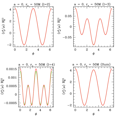
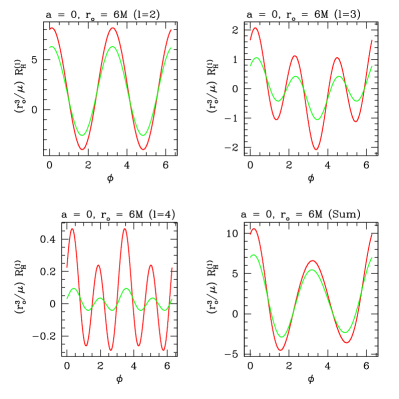
Figure 2: Comparison of numerically computed scalar curvature perturbation $R^{(1)}_{\rm H}$ for Schwarzschild with the analytic expansion given in Eqs. (125)–(136). The four panels on the left compare numerical (dark gray curves; red in color) and analytic (light gray; green in color) results for an orbit at $r_{\rm o}=50M$. Panels on the right are for $r_{\rm o}=6M$. In both cases, we plot $(r_{\rm o}^{3}/\mu)R^{(1)}_{\rm H}$, scaling out the leading dependence on orbital radius and the orbiting body’s mass. We show contributions for $l=2$, $l=3$, and $l=4$, plus the sum of these modes. For $r_{\rm o}=50M$, we have $u=0.14$, and we see very good agreement between the numerical and analytic formulas. In several cases, the numerical data lie on top of the analytic curves. For $r_{\rm o}=6M$, $u=0.41$, and the agreement is not as good. Although the amplitudes disagree in the strong field (especially for large $l$), the two computations maintain good phase agreement well into the strong field.

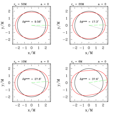
Figure 3: Equatorial section of the embedding of a distorted Schwarzschild horizon. Each panel shows the distortion for a different orbital radius, varying from $r_{\rm o}=50M$ to $r_{\rm o}=6M$. The black circles are the undistorted black hole, and the red curves are the distorted horizons, embedded with Eq. (142). These plots are in a frame that corotates with the orbit, and are for a slice of constant ingoing time $v$. The green dashed line in each panel shows the angle at which the tidal distortion is largest; the black dotted line shows the orbit’s position. Notice that the bulge leads the orbit in all cases, with the lead angle growing as the orbit moves to smaller orbital radius. We have rescaled the horizon’s tidal distortion by a factor $\propto r_{\rm o}^{3}/\mu$ so that, at leading order, the magnitude of the distortion is the same in all plots.

Figure 3 shows distorted black holes by embedding the horizon in a 3-dimensional Euclidean space, as discussed in Sec. III.1.2. Now, we do not truncate at $l=2$, but include all moments that we calculate. We show the equatorial slices of our embeddings for several different circular orbits ($r_{\rm o}=50M$, $20M$, $10M$, and $6M$). In all of our plots, we scale the horizon distortion $\varepsilon_{lm}$ by a factor proportional to $r_{\rm o}^{3}/\mu$ so that the tide’s impact is of roughly the same magnitude for all orbital separations.

The embeddings are shown in a frame that corotates with the orbit at an instant $v={\rm constant}$. The $x$-axis is at $\phi=0$, so the orbiting body sits at $\phi=\Delta\phi(r_{\rm o})=-\Omega_{\rm orb}r^{*}_{\rm o}$. In each panel, we have indicated where the radius of the embedding is largest (green dashed line, showing the angle of greatest tidal distortion) and the angular position of the orbiting body (black dotted line). In all cases, the bulge leads the orbiting body’s position, just as predicted in Sec. III.1.3. The numerical value of the bulge’s position relative to the orbit, $\delta\phi^{\rm num}$, agrees quite well with $\delta\phi^{\rm OB}_{22}$, Eq. (147) From Fig. 3, we have

$$\delta\phi^{\rm num} = 9.56^{\circ}\quad r_{\rm o}=50M\;,$$ (151)

$$= 17.3^{\circ}\quad r_{\rm o}=20M\;,$$

$$= 27.8^{\circ}\quad r_{\rm o}=10M\;,$$

$$= 37.6^{\circ}\quad r_{\rm o}=6M\;.$$

Equation (147) tells us

$$\delta\phi^{\rm OB}_{22} = 9.54^{\circ}\quad r_{\rm o}=50M\;,$$ (152)

$$= 17.1^{\circ}\quad r_{\rm o}=20M\;,$$

$$= 26.8^{\circ}\quad r_{\rm o}=10M\;,$$

$$= 35.0^{\circ}\quad r_{\rm o}=6M\;.$$

In all cases, the true position of the bulge is slightly larger than $\delta\phi^{\rm OB}_{22}$. This appears to be due in large part to the contribution of modes other than $l=|m|=2$; the agreement improves if we calculate $\delta\phi^{\rm num}$ using only the $l=2$ contribution to the embedding.

IV Results II: Kerr

Now consider non-zero black hole spin. We begin with slow motion and small black hole spin, expanding Eq. (LABEL:eq:gauss_kerr) using $u\equiv(M/r_{\rm o})^{1/2}\ll 1$ and $q\equiv a/M\ll 1$, and derive analytic results which are useful points of comparison to the general case. We then show numerical results which illustrate tidal deformations for strong-field orbits.

IV.1 Slow motion: Analytic results

Here we present analytic results, expanding in powers of $u=(M/r_{\rm o})^{1/2}$ and $q=a/M$. We take all relevant quantities to order $u^{5}$ and $q$ beyond the leading term; this is far enough to see how quantities behave for $l\leq 4$. We compare with strong-field numerical results in the following subsection.

Begin again with ${\cal C}_{lm}$. Neglect the $k$ and $n$ indices which are irrelevant for circular, equatorial orbits, and expand $\lambda=\lambda_{0}+(a\omega_{m})\lambda_{1}$, with $\lambda_{0}$ and $\lambda_{1}$ given by Eqs. (325) and (327) for $s=-2$ [recall that $\lambda$ comes from the spheroidal harmonic $S^{-}_{lm}(\theta)$]. Finally, expand to $O(u^{5})$ and $O(q)$. Doing so, Eq. (39) yields

$${\cal C}_{2m} = -\frac{16i}{3}M^{2}\left(1-\frac{13}{3}qm^{2}u^{3}\right)\exp\left[-im\left(\frac{13}{2}u^{3}-\frac{3}{2}q\right)\right]\;,$$ (153)

$${\cal C}_{3m} = -\frac{16i}{15}M^{2}\left(1-\frac{14}{3}qm^{2}u^{3}\right)\exp\left[-im\left(\frac{61}{10}u^{3}-\frac{3}{2}q\right)\right]\;,$$ (154)

$${\cal C}_{4m} = -\frac{16i}{45}M^{2}\left(1-\frac{24}{5}qm^{2}u^{3}\right)\exp\left[-im\left(\frac{181}{30}u^{3}-\frac{3}{2}q\right)\right]\;.$$ (155)

These reduce to the Schwarzschild results, Eqs. (110) – (112), when $q\to 0$.

Next, the amplitudes $Z^{\rm H}_{lm}$, again following the algorithm described in Sec. II.2. These results should be understood to neglect contributions of $O(u^{6})$, $O(q^{2})$ and higher. As elsewhere, $\mu$ is the mass of the smaller body. For $l=2$, we have

$$Z^{\rm H}_{20} = \sqrt{\frac{3\pi}{10}}\frac{\mu}{r_{\rm o}^{3}}\left(1+\frac{7}{2}u^{2}-4qu^{3}+\frac{561}{56}u^{4}-18qu^{5}\right)\;,$$ (156)

$$Z^{\rm H}_{21} = -3i\sqrt{\frac{\pi}{5}}\frac{\mu}{r_{\rm o}^{3}}\biggl{\{}\left(1-\frac{i}{2}q\right)u-\frac{2}{3}qu^{2}+\left(\frac{8}{3}-\frac{4i}{3}q\right)u^{3}+\left[\frac{10i}{3}+\left(\frac{1}{6}-\frac{\pi^{2}}{3}\right)q\right]u^{4}+\left(\frac{152}{21}-\frac{368}{63}q\right)u^{5}\biggr{\}}$$ (157)

$$= -3i\sqrt{\frac{\pi}{5}}\frac{\mu}{r_{\rm o}^{3}}\biggl{[}u-\frac{2}{3}qu^{2}+\frac{8}{3}u^{3}-\left(\frac{3}{2}+\frac{\pi^{2}}{3}\right)qu^{4}+\frac{152}{21}u^{5}\biggr{]}\exp\left[i\left(\frac{10}{3}u^{3}-\frac{q}{2}\right)\right]\;,$$

$$Z^{\rm H}_{22} = -\frac{3}{2}\sqrt{\frac{\pi}{5}}\frac{\mu}{r_{\rm o}^{3}}\biggl{\{}1-iq+\left(\frac{3}{2}-\frac{3i}{2}q\right)u^{2}+\left[\frac{23i}{3}+\left(15-\frac{4\pi^{2}}{3}\right)q\right]u^{3}+\left(\frac{1403}{168}-\frac{1403i}{168}q\right)u^{4}$$

$$+\left[\frac{473i}{30}+\left(\frac{2449}{90}-2\pi^{2}\right)q\right]u^{5}\biggr{\}}$$

$$= -\frac{3}{2}\sqrt{\frac{\pi}{5}}\frac{\mu}{r_{\rm o}^{3}}\biggl{[}1+\frac{3}{2}u^{2}+\left(\frac{22}{3}-\frac{4\pi^{2}}{3}\right)qu^{3}+\frac{1403}{168}u^{4}+\left(\frac{103}{9}-2\pi^{2}\right)qu^{5}\biggr{]}\exp\left[i\left(\frac{23}{3}u^{3}+\frac{64}{15}u^{5}-q\right)\right]\;.$$

For $l=3$,

$$Z^{\rm H}_{30} = -i\sqrt{\frac{30\pi}{7}}\frac{\mu}{r_{\rm o}^{3}}\left(u^{3}-\frac{3}{4}qu^{4}+4u^{5}\right)\;,$$ (159)

$$Z^{\rm H}_{31} = -\frac{3}{2}\sqrt{\frac{5\pi}{14}}\frac{\mu}{r_{\rm o}^{3}}\left\{\left(1-\frac{i}{6}q\right)u^{2}+\left(\frac{13}{3}-\frac{13i}{18}q\right)u^{4}+\left[\frac{43i}{30}-\left(\frac{247}{180}+\frac{\pi^{2}}{3}\right)q\right]u^{5}\right\}$$ (160)

$$= -\frac{3}{2}\sqrt{\frac{5\pi}{14}}\frac{\mu}{r_{\rm o}^{3}}\left[u^{2}+\frac{13}{3}u^{4}-\left(\frac{29}{18}+\frac{\pi^{2}}{3}\right)qu^{5}\right]\exp\left[i\left(\frac{43}{30}u^{3}-\frac{q}{6}\right)\right]\;,$$

$$Z^{\rm H}_{32} = 5i\sqrt{\frac{\pi}{7}}\frac{\mu}{r_{\rm o}^{3}}\left[\left(1-\frac{i}{3}q\right)u^{3}-\frac{3}{4}qu^{4}+4\left(1-\frac{i}{3}q\right)u^{5}\right]$$ (161)

$$= 5i\sqrt{\frac{\pi}{7}}\frac{\mu}{r_{\rm o}^{3}}\left(u^{3}-\frac{3}{4}qu^{4}+4u^{5}\right)\exp\left(-iq/3\right)\;,$$

$$Z^{\rm H}_{33} = \frac{5}{2}\sqrt{\frac{3\pi}{14}}\frac{\mu}{r_{\rm o}^{3}}\left\{\left(1-\frac{i}{2}q\right)u^{2}+\left(3-\frac{3i}{2}q\right)u^{4}+\left[\frac{43i}{10}+\left(\frac{393}{20}-3\pi^{2}\right)q\right]u^{5}\right\}$$ (162)

$$= \frac{5}{2}\sqrt{\frac{3\pi}{14}}\frac{\mu}{r_{\rm o}^{3}}\left[u^{2}+3u^{4}+\left(\frac{35}{2}-3\pi^{2}\right)qu^{5}\right]\exp\left[i\left(\frac{43}{10}u^{3}-\frac{q}{2}\right)\right]\;.$$

And for $l=4$,

$$Z^{\rm H}_{40}=-\frac{9}{14}\sqrt{\frac{5\pi}{2}}\frac{\mu}{r_{\rm o}^{3}}u^{4}\;,$$ (163)

$$Z^{\rm H}_{41}=\frac{45i}{14}\sqrt{\frac{\pi}{2}}\frac{\mu}{r_{\rm o}^{3}}\left[\left(1+\frac{i}{12}q\right)u^{5}\right]=\frac{45i}{14}\sqrt{\frac{\pi}{2}}\frac{\mu}{r_{\rm o}^{3}}u^{5}\exp\left(iq/12\right)\;,$$ (164)

$$Z^{\rm H}_{42}=\frac{15}{14}\sqrt{\pi}\frac{\mu}{r_{\rm o}^{3}}\left[\left(1+\frac{i}{6}q\right)u^{4}\right]=\frac{15}{14}\sqrt{\pi}\frac{\mu}{r_{\rm o}^{3}}u^{4}\exp\left(iq/6\right)\;,$$ (165)

$$Z^{\rm H}_{43}=-\frac{15i}{2}\sqrt{\frac{\pi}{14}}\frac{\mu}{r_{\rm o}^{3}}\left[\left(1+\frac{i}{4}q\right)u^{5}\right]=-\frac{15i}{2}\sqrt{\frac{\pi}{14}}\frac{\mu}{r_{\rm o}^{3}}u^{5}\exp\left(iq/4\right)\;,$$ (166)

$$Z^{\rm H}_{44}=-\frac{15}{4}\sqrt{\frac{\pi}{7}}\frac{\mu}{r_{\rm o}^{3}}\left[\left(1+\frac{i}{3}q\right)u^{4}\right]=-\frac{15}{4}\sqrt{\frac{\pi}{7}}\frac{\mu}{r_{\rm o}^{3}}u^{4}\exp\left(iq/3\right)\;.$$ (167)

Equations (156) – (167) reduce to Eqs. (113) – (124) when $q\to 0$. Modes for $m<0$ can be obtained using the rule $Z^{\rm H}_{l-m}=(-1)^{l}\bar{Z}^{\rm H}_{lm}$, with overbar denoting complex conjugate.

Lastly, we need the angular function $\bar{\eth}\bar{\eth}S^{+}_{lm}$ to leading order in $q$. Using Eqs. (66), (67), (72), and the condition $q\ll 1$, we have

$$\bar{\eth}\bar{\eth}S^{+}_{lm}=\frac{1}{8M^{2}}L_{-}^{s}L_{-}^{s}\left(1+iq\cos\theta\right)S^{+}_{lm}=\frac{1}{8M^{2}}\left[(1+iq\cos\theta)L_{-}^{s}L_{-}^{s}S^{+}_{lm}-2iq\sin\theta L_{-}^{s}S^{+}_{lm}\right]\;.$$ (168)

Following the analysis in Appendix C, the spheroidal harmonic to this order is

$$S^{+}_{lm}={{}_{2}}Y_{lm}+qM\omega_{m}\left[c^{l+1}_{lm}{{}_{2}}Y_{(l+1)m}+c^{l-1}_{lm}{{}_{2}}Y_{(l-1)m}\right]\;,$$ (169)

where

$$c^{l+1}_{lm} = -\frac{2}{(l+1)^{2}}\sqrt{\frac{(l+3)(l-1)(l+m+1)(l-m+1)}{(2l+3)(2l+1)}}\;,$$ (170)

$$c^{l-1}_{lm} = \frac{2}{l^{2}}\sqrt{\frac{(l+2)(l-2)(l+m)(l-m)}{(2l+1)(2l-1)}}\;.$$ (171)

Using Eq. (63) with Eqs. (168) and (169) and expanding to leading order in $q$, we find

$$\bar{\eth}\bar{\eth}S^{+}_{lm} = \frac{1}{8M^{2}}\biggl{[}(1+iq\cos\theta)\sqrt{(l+2)(l+1)l(l-1)}\,{{}_{0}}Y_{lm}-2iq\sin\theta\sqrt{(l+2)(l-1)}\,{{}_{1}}Y_{lm}$$ (172)

$$\qquad+qM\omega_{m}\left(c^{l+1}_{lm}\sqrt{(l+3)(l+2)(l+1)l}\,{{}_{0}}Y_{(l+1)m}+c^{l-1}_{lm}\sqrt{(l+1)l(l-1)(l-2)}\,{{}_{0}}Y_{(l-1)m}\right)\biggr{]}\;.$$

As in Sec. III.1, it is convenient to combine modes in pairs. For $l=2$, we find

$$R^{(1)}_{{\rm H},20} = -\frac{\mu}{r_{\rm o}^{3}}\left(3\cos^{2}\theta-1\right)\left(1+\frac{7}{2}u^{2}-4qu^{3}+\frac{561}{56}u^{4}-18qu^{5}\right)\;,$$ (173)

$$R^{(1)}_{{\rm H},2-1}+R^{(1)}_{{\rm H},21} = \frac{4\mu}{r_{\rm o}^{3}}\left(5\cos^{2}\theta-1\right)\sin\theta\,q\left(u+\frac{8}{3}u^{3}+\frac{152}{21}u^{5}\right)\cos\left(\psi-\Omega_{\rm orb}v-\frac{3}{2}u^{3}+6M\Omega_{\rm H}\right)\;,$$ (174)

$$R^{(1)}_{{\rm H},2-2}+R^{(1)}_{{\rm H},22} = \frac{3\mu}{r_{\rm o}^{3}}\sin^{2}\theta\left[1+\frac{3}{2}u^{2}-\left(10+\frac{4\pi^{2}}{3}\right)qu^{3}+\frac{1403}{168}u^{4}-\left(\frac{131}{9}+2\pi^{2}\right)qu^{5}\right]\times$$ (175)

$$\quad\cos\left[2\left(\psi-\Omega_{\rm orb}v-\frac{8}{3}u^{3}+\frac{32}{5}u^{5}+\frac{14}{3}M\Omega_{\rm H}\right)\right]\;.$$

For $l=3$,

$$R^{(1)}_{{\rm H},30} = -\frac{\mu}{r_{\rm o}^{3}}\left(1-12\cos^{2}\theta+15\cos^{4}\theta\right)qu^{3}(1+4u^{2})\;,$$ (176)

$$R^{(1)}_{{\rm H},3-1}+R^{(1)}_{{\rm H},31} = \frac{3}{2}\frac{\mu}{r_{\rm o}^{3}}\sin\theta\left(1-5\cos^{2}\theta\right)u^{2}\left[1+\frac{13}{3}u^{2}-\left(\frac{113}{12}+\frac{\pi^{2}}{2}\right)qu^{3}\right]\cos\left[\psi-\Omega_{\rm orb}v-\frac{14}{3}u^{3}+\frac{20}{3}M\Omega_{\rm H}\right]\;,$$

$$R^{(1)}_{{\rm H},3-2}+R^{(1)}_{{\rm H},32} = \frac{5}{3}\frac{\mu}{r_{\rm o}^{3}}q(u^{3}+4u^{5})\left\{9\cos^{2}\theta\cos\left[2\left(\psi-\Omega_{\rm orb}v-\frac{56}{10}u^{3}+\frac{22}{3}M\Omega_{\rm H}\right)\right]\right.$$ (178)

$$\qquad\qquad\qquad\qquad\left.-\cos\left[2\left(\psi-\Omega_{\rm orb}v-\frac{158}{30}u^{3}+\frac{22}{3}M\Omega_{\rm H}\right)\right]\right\}\;,$$

$$R^{(1)}_{{\rm H},3-3}+R^{(1)}_{{\rm H},33} = \frac{5}{2}\frac{\mu}{r_{\rm o}^{3}}\sin^{3}\theta u^{2}\left[1+3u^{2}-\left(\frac{49}{2}+3\pi^{2}\right)qu^{3}\right]\cos\left[3\left(\psi-\Omega_{\rm orb}v-\frac{14}{3}u^{3}+\frac{20}{3}M\Omega_{\rm H}\right)\right]\;.$$

And for $l=4$,

$$R^{(1)}_{{\rm H},40} = \frac{9}{56}\frac{\mu}{r_{\rm o}^{3}}\left(3-30\cos^{2}\theta+35\cos^{4}\theta\right)u^{4}\;,$$ (180)

$$R^{(1)}_{{\rm H},4-1}+R^{(1)}_{{\rm H},41} = -\frac{9}{28}\frac{\mu}{r_{\rm o}^{3}}\sin\theta\,qu^{5}\left[98\cos^{4}\theta\cos\left(\psi-\Omega_{\rm orb}v-\frac{169}{30}u^{3}+\frac{25}{3}M\Omega_{\rm H}\right)\right.$$

$$\quad\left.-57\cos^{2}\theta\cos\left(\psi-\Omega_{\rm orb}v-\frac{1568}{285}u^{3}+\frac{25}{3}M\Omega_{\rm H}\right)+3\cos\left(\psi-\Omega_{\rm orb}v-\frac{77}{15}u^{3}+\frac{25}{3}M\Omega_{\rm H}\right)\right]\;,$$

$$R^{(1)}_{{\rm H},4-2}+R^{(1)}_{{\rm H},42} = \frac{15}{14}\frac{\mu}{r_{\rm o}^{3}}\sin^{2}\theta\left(1-7\cos^{2}\theta\right)u^{4}\cos\left[2\left(\psi-\Omega_{\rm orb}v-\frac{181}{30}u^{3}+\frac{119}{15}M\Omega_{\rm H}\right)\right]\;,$$ (182)

$$R^{(1)}_{{\rm H},4-3}+R^{(1)}_{{\rm H},43} = \frac{3}{4}\frac{\mu}{r_{\rm o}^{3}}\sin^{3}\theta\,qu^{5}\left\{14\cos^{2}\theta\cos\left[3\left(\psi-\Omega_{\rm orb}v-\frac{169}{30}u^{3}+\frac{25}{3}M\Omega_{\rm H}\right)\right]\right.$$ (183)

$$\quad\qquad\qquad\qquad\left.-\cos\left[3\left(\psi-\Omega_{\rm orb}v-\frac{77}{15}u^{3}+\frac{25}{3}M\Omega_{\rm H}\right)\right]\right\}\;,$$

$$R^{(1)}_{{\rm H},4-4}+R^{(1)}_{{\rm H},44} = \frac{15}{8}\frac{\mu}{r_{\rm o}^{3}}\sin^{4}\theta u^{4}\cos\left[4\left(\psi-\Omega_{\rm orb}v-\frac{181}{30}u^{3}+\frac{119}{15}M\Omega_{\rm H}\right)\right]\;.$$ (184)

In writing these formulas, we have used the fact that $\Omega_{\rm H}=q/4M$ in the $q\ll 1$ limit to rewrite certain terms in the phases using $\Omega_{\rm H}$ rather than $q$. For example, in Eq. (175) our calculation yields a term $7q/6$ in the argument of the cosine, which we rewrite $14M\Omega_{\rm H}/3$. We have found that this improves the match of Eqs. (173) – (184) with the numerical results we discuss in Sec. IV.2.

IV.1.1 Phase of the tidal bulge: Null map

We begin by examining the bulge-orbit offset using the null map, Eq. (LABEL:eq:bulge_vs_orbit_null). The horizon’s geometry is dominated by contributions for which $l+m$ is even; modes with $l+m$ odd are suppressed by $qu$ relative to these dominant modes (thus vanishing in the Schwarzschild limit). The dominant modes peak at $\psi^{\rm bulge}_{lm}=\Omega_{\rm orb}v+\delta\psi_{lm}(u)+\delta\psi_{lm}(q)$, where $\delta\psi_{lm}(u)$ and $\delta\psi_{lm}(q)$ can be read out of Eqs. (173) – (184). The orbit mapped onto the horizon in the null map is given by Eq. (81). Following discussion in Sec. II.4.1, the offset phases in the null map for the dominant modes, to $O(u^{5})$ and $O(q)$, are

$$\delta\psi^{\rm OB-NM}_{22} = \frac{8}{3}\left(u^{3}-M\Omega_{\rm H}\right)-\frac{32}{5}u^{5}-\frac{4M^{2}\Omega_{\rm H}}{r_{\rm o}}$$ (185)

$$-\Delta\psi(r_{\rm o})\;,$$

$$\delta\psi^{\rm OB-NM}_{31} = \delta\psi^{\rm OB-NM}_{33}$$

$$= \frac{14}{3}\left(u^{3}-M\Omega_{\rm H}\right)-\frac{4M^{2}\Omega_{\rm H}}{r_{\rm o}}-\Delta\psi(r_{\rm o})\;,$$

$$\delta\psi^{\rm OB-NM}_{42} = \delta\psi^{\rm OB-NM}_{44}$$

$$= \frac{181}{30}u^{3}-\frac{89}{15}M\Omega_{\rm H}-\frac{4M^{2}\Omega_{\rm H}}{r_{\rm o}}-\Delta\psi(r_{\rm o})\;.$$

We again see agreement with Fang and Lovelace for $l=m=2$, who correct a sign error in Hartle’s hartle74 treatment of the bulge phase; compare Eq. (61) and footnote 6 of Ref. fl05 and associated discussion. In contrast to the Schwarzschild case, the Kerr offset phases can be positive or negative, depending on the values of $r_{\rm o}$ and $q$. To highlight this further, let us examine Eq. (185) for very large $r_{\rm o}$: we drop the term in $u^{5}$, and expand $\Delta\psi(r_{\rm o})$. The result is

$$\delta\psi^{\rm OB-NM}_{22}\simeq\frac{8}{3}\left(u^{3}-M\Omega_{\rm H}\right)+\sqrt{\frac{M}{r_{\rm o}}}\;.$$ (188)

As $r_{\rm o}\to\infty$, we see that this bulge lags the orbit by $\delta^{\rm OB-NM}_{22}=-8M\Omega_{\rm H}/3$, which reproduces Hartle’s finding for a stationary moon orbiting a slowly rotating Kerr black hole [Eq. (4.34) of Ref. hartle74 , correcting the sign error discussed in footnote 6 of Ref. fl05 ]. We discuss this point further in Sec. V.

IV.1.2 Phase of the tidal bulge: Instantaneous map

Consider next the instantaneous-in-$v$ map discussed in Sec. II.4.2. The position of the orbit on the horizon in this mapping is given by Eq. (85). To $O(u^{5})$ and $O(q)$, the offset phase for the dominant modes in this map is

$$\delta\psi^{\rm OB-IM}_{22} = \frac{8}{3}u^{3}-\frac{14}{3}M\Omega_{\rm H}-\frac{32}{5}u^{5}-\Delta\psi(r_{\rm o})\;,$$

$$\delta\psi^{\rm OB-IM}_{31} = \delta\psi^{\rm OB-IM}_{33}$$ (190)

$$= \frac{14}{3}u^{3}-\frac{20}{3}M\Omega_{\rm H}-\Delta\psi(r_{\rm o})\;,$$

$$\delta\psi^{\rm OB-IM}_{42} = \delta\psi^{\rm OB-IM}_{44}$$ (191)

$$= \frac{181}{30}u^{3}-\frac{119}{15}M\Omega_{\rm H}-\Delta\psi(r_{\rm o})\;.$$

As in the null map, these phases can be positive or negative, depending on the values of $r_{\rm o}$ and $q$. As we’ll see when we examine numerical results for the horizon geometry, Eq. (LABEL:eq:psi_obim_2) does a good job describing the angle of the peak horizon bulge for small values of $q$.

IV.1.3 Phase of the tidal bulge: Tidal field versus tidal response

Finally, let us examine the relative phase of tidal field modes $\psi^{\rm HH}_{0,lm}$ and the horizon’s response $R^{(1)}_{{\rm H},lm}$. For $q\ll 1$, we have $\kappa^{-1}=4M+O(q^{2})$. Expanding in the weak-field limit, Eq. (91) becomes

$$\delta\psi^{\rm TB}_{lm}=4m(u^{3}-M\Omega_{\rm H})+{\cal S}_{lm}(\pi/2)\;.$$ (192)

For the modes with $l+m$ even which dominate the horizon’s response, it is not difficult to compute ${\cal S}_{lm}(\pi/2)$ to leading order in $q$. Equation (172) and the definition (90) yield

$${\cal S}_{lm}(\pi/2)=\frac{2q}{\sqrt{l(l+1)}}\frac{{{}_{1}}Y_{lm}(\pi/2)}{{{}_{0}}Y_{lm}(\pi/2)}+O(q^{2})\;.$$ (193)

We also know [cf. Eq. (A8) of Ref. h2000 ] that

$${{}_{1}}Y_{lm}(\theta)=-\frac{1}{\sqrt{l(l+1)}}\left(\partial_{\theta}-m\csc\theta\right){{}_{0}}Y_{lm}(\theta)\;.$$ (194)

For $l+m$ even, $\partial_{\theta}\,{{}_{0}}Y_{lm}=0$ at $\theta=\pi/2$. Plugging the resulting expression for ${{}_{1}}Y_{lm}(\pi/2)$ into Eq. (193), we find

$${\cal S}_{lm}(\pi/2)=\frac{2mq}{l(l+1)}=\frac{8mM\Omega_{\rm H}}{l(l+1)}\;,$$ (195)

where in the last step we again used $q=4M^{2}\Omega_{\rm H}$, accurate for $q\ll 1$. With this, Eq. (192) becomes

$$\delta\psi^{\rm TB}_{lm} = 4m\left[u^{3}-M\Omega_{\rm H}\left(1-\frac{2}{l(l+1)}\right)\right]$$ (196)

$$= 4m\left[u^{3}-M\Omega_{\rm H}\frac{(l+2)(l-1)}{l(l+1)}\right]\;.$$

Just as with the offset phases of the bulge and the orbit for Kerr, this tidal bulge phase can be either positive or negative depending on $r_{\rm o}$ and $q$, and so the horizon’s response can lead or lag the applied tidal field.

IV.2 Fast motion: Numerical results

Figures 4, 5, and 6 present summary data for our numerical calculations of tidally distorted Kerr black holes. Just as in Sec. III.2, we compute $R^{(1)}_{\rm H}$ by solving for $Z^{\rm H}_{lm}$ as described in Sec. II.2, and then apply Eq. (LABEL:eq:gauss_kerr). As in the Schwarzschild case, we find rapid convergence with mode index $l$. All the data we show are for the equatorial plane, $\theta=\pi/2$, and are rescaled by $(r_{\rm o}^{3}/\mu)$. We typically include all modes up to $l=15$ (increasing this to $20$ and $25$ in a few very strong field cases). Contributions beyond this are typically at the level of $10^{-9}$ or smaller, which is accurate enough for this exploratory analysis.

Figure 4 is the Kerr analog of Fig. 2, comparing numerical results for $R^{\rm H}_{lm}$ with analytic predictions for selected black hole spins, mode numbers, and orbital radii. For all modes we show here, we see outstanding agreement in both phase and amplitude for $q=0.1$ and $r_{\rm o}=50M$; in some cases, the numerical data lies almost directly on top of the analytic prediction. The amplitude agreement is not quite as good as we increase the spin to $q=0.2$ and move to smaller radius ($r_{\rm o}=10M$), though the phase agreement remains quite good for all modes.

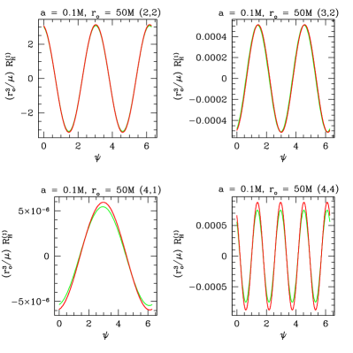
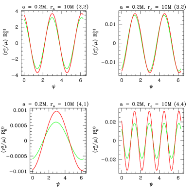
Figure 4: Comparison of selected modes for the numerically computed scalar curvature perturbation $R^{(1)}_{{\rm H},lm}$ with the analytic expansion given in Eqs. (173) – (184). The four panels on the left are for orbits of a black hole with $a=0.1M$ at $r_{\rm o}=50M$; those on the right are for orbits of a black hole with $a=0.2M$ at $r_{\rm o}=10M$. The mode shown is indicated by $(l,m)$ in the upper right corner of each panel [we actually show the contributions from $(l,m)$ and $(l,-m)$]. In all cases, we plot $(r_{\rm o}^{3}/\mu)R^{(1)}_{\rm H}$, scaling out the leading dependence on orbital radius and the orbiting body’s mass. Curves in light gray (green in color) are the analytic results, those in dark gray (red in color) are our numerical data. Agreement for the large radius, low spin cases is extremely good, especially for small $l$ where the numerical data lies practically on top of the analytic predictions. As we increase $q$ and decrease $r_{\rm o}$, the amplitude agreement becomes less good, though the analytic formulas still are within several to several tens of percent of the numerical data. The phase agreement is outstanding in all of these cases.

Figures 5 and 6 show equatorial slices of the embedding of distorted Kerr black holes for a range of orbits and black hole spins. These embeddings are similar to those we used for distorted Schwarzschild black holes (as described in Sec. III.1.2), with a few important adjustments. The embedding surface we use has the form

$$r_{\rm E}=r_{\rm E}^{0}(\theta)+r_{+}\sum_{\ell m}\varepsilon_{\ell m}(\theta,\psi)\;.$$ (197)

Both the undistorted radius $r_{\rm E}^{(0)}(\theta)$ and the tidal distortion $\varepsilon_{\ell m}(\theta,\psi)$ are described in Appendix B; see also Ref. smarr . The background embedding reduces to a sphere of radius $2M$ when $a=0$, but is more complicated in general. The embedding’s tidal distortion is linearly related to the curvature $R^{(1)}_{{\rm H},lm}$, but in a way that is more complicated than the Schwarzschild relation (142). In particular, mode mixing becomes important: Different angular basis functions are needed to describe the curvature $R^{(1)}_{{\rm H},lm}$ and the embedding distortion $\varepsilon_{\ell m}$ when $a\neq 0$. Hence, the $\ell=2$ contribution to the horizon’s shape has contributions from all $l$ curvature modes, not just $l=2$. See Appendix B for detailed discussion.

In this paper, we only generate embeddings for $a/M\leq\sqrt{3}/2$. For spins greater than this, the horizon cannot be embedded in a global 3-dimensional Euclidean space. A “belt” from $\pi-\theta_{\rm E}\leq\theta\leq\theta_{\rm E}$ can always be embedded in 3-dimensional Euclidean space, but the “polar cones” $0\leq\theta<\theta_{\rm E}$ and $\pi-\theta_{\rm E}<\theta\leq\pi$ must be embedded in a Lorentzian geometry (where $\theta_{\rm E}$ is related to the root of a function used in the embedding; see Appendix B for details). Alternatively, one can embed the entire horizon in a different space, as discussed in Refs. frolov ; gibbons . We defer detailed discussion of embeddings that can handle the case $a/M>\sqrt{3}/2$ to a later paper.

As with the Schwarzschild embeddings shown in Fig. 3, the Kerr embeddings we show are all plotted in a frame that corotates with the orbit at a moment $v={\rm constant}$. The $x$-axis is at $\psi=0$, and the orbiting body sits at $\psi=\Delta\psi(r_{\rm o})=\bar{r}_{\rm o}-\Omega_{\rm orb}r^{*}_{\rm o}$. As in Fig. 3, the green dashed line labels the horizon’s peak bulge, and the black dotted line shows the position of the orbiting body.

For small $q$, we find that the numerically computed bulge offset agrees quite well with the $l=2$ analytic expansion in the instantaneous map, Eq. (LABEL:eq:psi_obim_2). For $q=0.1$, our numerical results are

$$\delta\psi^{\rm num} = 3.01^{\circ}\quad r_{\rm o}=50M\;,$$ (198)

$$= 10.8^{\circ}\quad r_{\rm o}=20M\;,$$

$$= 21.6^{\circ}\quad r_{\rm o}=10M\;,$$

$$= 33.7^{\circ}\quad r_{\rm o}=5.669M\;.$$

These are within a few percent of predictions based on the weak-field, slow spin expansion:

$$\delta\psi^{\rm OB-IM}_{22} = 2.95^{\circ}\quad r_{\rm o}=50M\;,$$ (199)

$$= 10.7^{\circ}\quad r_{\rm o}=20M\;,$$

$$= 20.6^{\circ}\quad r_{\rm o}=10M\;,$$

$$= 30.0^{\circ}\quad r_{\rm o}=5.669M\;.$$

As we move to larger spin, the agreement rapidly becomes worse. Terms which we neglect in our expansion become important, and the mode mixing described above becomes very important. For $q=0.4$, the agreement degrades to a few tens of percent in most cases:

$$\delta\psi^{\rm num} = -13.5^{\circ}\quad r_{\rm o}=50M\;,$$ (200)

$$= -6.17^{\circ}\quad r_{\rm o}=20M\;,$$

$$= 3.55^{\circ}\quad r_{\rm o}=10M\;,$$

$$= 21.4^{\circ}\quad r_{\rm o}=4.614M\;;$$

and

$$\delta\psi^{\rm OB-IM}_{22} = -17.9^{\circ}\quad r_{\rm o}=50M\;,$$ (201)

$$= -9.76^{\circ}\quad r_{\rm o}=20M\;,$$

$$= 0.82^{\circ}\quad r_{\rm o}=10M\;,$$

$$= 13.6^{\circ}\quad r_{\rm o}=4.614M\;.$$

The agreement gets significantly worse as $q$ is increased further. Presumably, $q\sim 0.3$ is about as far as the leading order expansion in $q$ can reasonably be taken.

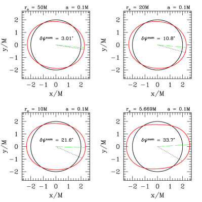
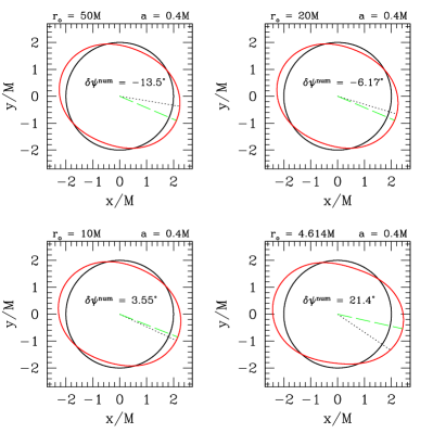
Figure 5: Equatorial section of the embedding of distorted Kerr black hole event horizons, $a=0.1M$ and $a=0.4M$. Each panel represents the distortion for a different radius of the orbiting body, varying from $r_{\rm o}=50M$ to the innermost stable circular orbit ($r_{\rm o}=5.669M$ for $a=0.1M$, $r_{\rm o}=4.614M$ for $a=0.4M$). As in Fig. 3, the green dashed line shows the angle at which the tidal distortion is largest, and the black dotted line shows the position of the orbit. As in Fig. 3, we have rescaled by a factor $\propto r_{\rm o}^{3}/\mu$ to account for the leading dependence of the tide on mass and orbital separation. In contrast to the Schwarzschild results, the bulge does not lead the orbit in all cases here. The amount by which the bulge leads the orbit grows as the orbit moves to small orbital radius (in some cases, changing from a lag to a lead as part of this trend).

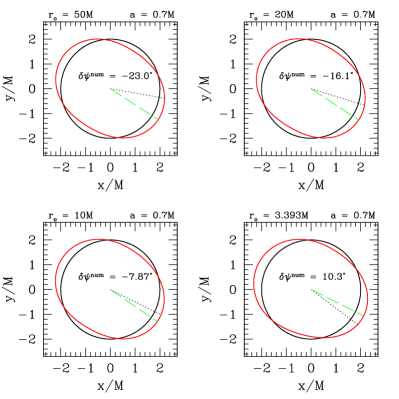
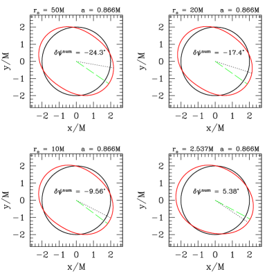
Figure 6: Equatorial section of the embedding of distorted Kerr black hole event horizons, $a=0.7M$ and $a=0.866M$. Each panel represents the distortion for a different radius of the orbiting body, varying from $r_{\rm o}=50M$ to the innermost stable circular orbit ($r_{\rm o}=3.393M$ for $a=0.7M$, $r_{\rm o}=2.537M$ for $a=0.866M$), with the green dashed and black dotted lines labeling the locations of maximal distortion and position of the orbit, respectively, and with the distortion rescaled by a factor $\propto r_{\rm o}^{3}/\mu$. The bulge lags the orbit in most cases we show here, with the lag angle getting smaller and converting to a small lead as the orbit moves to smaller and smaller orbital radius.

To conclude this section, we show two examples of embeddings for the entire horizon surface, rather than just the equatorial slice. The left-hand panel of Fig. 7 is an example of a relatively mild tidal distortion. The black hole has spin $a=0.3M$, and the orbiting body is at $r_{\rm o}=20M$. The distortion is strongly dominated by the $\ell=2$ contribution, and we see a fairly simple prolate ellipsoid whose bulge lags the orbit. The right-hand panel shows a much more extreme example. The black hole here has $a=0.866M$, and the orbiting body is at $r_{\rm o}=1.75M$. The horizon’s shape has strong contributions from many multipoles, and so is bent in a rather more complicated way than in the mild case. The connection between the orbit and the horizon geometry is quite unusual here. Note that this extreme case corresponds to an unstable circular orbit, and so one might question whether this figure is physically relevant. We include it because we expect similar horizon distortions for very strong field orbits of black holes with $a/M>\sqrt{3}/2$, and that such a horizon geometry will be produced transiently from the closest approach of eccentric orbits around black holes with $a/M\lesssim\sqrt{3}/2$. Both of these cases will be investigated more thoroughly in later papers.

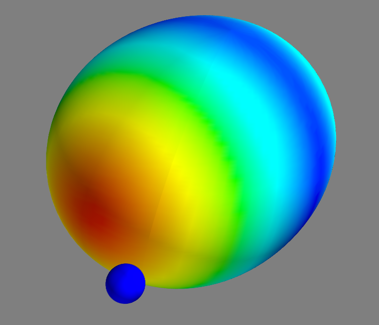
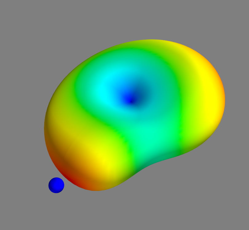
Figure 7: Two example embeddings of the tidally distorted horizon’s surface. Both panels show the 3-dimensional Euclidean embedding surface, $r_{\rm E}(\theta,\psi)$; the shading (or color scale) indicates the horizon’s distortion relative to an isolated Kerr black hole. The hole is stretched (i.e., $r_{\rm E}$ increased by the tides relative to an isolated hole; red in color) at the end near to and opposite from the orbiting body. It is squeezed ($r_{\rm E}$ decreased by tides; blue in color) in a band between these two ends. As in other figures illustrating the embedded distorted horizon, we have rescaled the distortion by a factor $\propto r_{\rm o}^{3}/\mu$. On the left, we show a relatively gentle deformation around a moderately spinning black hole: $a=0.3M$, $r_{\rm o}=20M$. The distortion here is dominated by a quadrupolar deformation of the horizon (lagging the orbiting body, whose angular position is indicated by the small blue ball). On the right, we show a rather extreme case: $a=0.866M$, $r_{\rm o}=1.75M$. The deformation here is much more complicated, as many multipoles beyond $l=2$ contribute to the shape of the horizon.

V Lead or lag?

We showed in Sec. II.5 that the orbital energy evolves due to horizon coupling according to $dE^{\rm H}/dt\propto(\Omega_{\rm orb}-\Omega_{\rm H})$. As discussed in the Introduction, it is simple to build an intuitive picture of this in Newtonian physics. For a Newtonian tide acting on a fluid body, when $\Omega_{\rm H}>\Omega_{\rm orb}$ tidal forces raise a bulge on the body which leads the orbit’s position. This bulge exerts a torque which transfers energy from the body’s spin to the orbit. When $\Omega_{\rm H}<\Omega_{\rm orb}$, the bulge lags the orbit, and the torque transfers energy from the orbit to the body’s spin. When $\Omega_{\rm H}=\Omega_{\rm orb}$, $dE^{\rm H}/dt=0$. The Newtonian fluid expectation is thus that there should be no offset between the bulge and the orbit. The tidal bulge should point directly at the orbiting body, locking the body’s tide to the orbit.

Consider now a fully relativistic calculation of tides acting on a black hole. When $\Omega_{\rm orb}\gg\Omega_{\rm H}$ (e.g., the Schwarzschild limit) and $\Omega_{\rm H}\gg\Omega_{\rm orb}$ (large radius orbits of Kerr black holes), the Newtonian fluid intuition is consistent with our results, modulo the switch of “lead” and “lag” thanks to the teleological nature of the event horizon. However, it is not so clear if this intuition holds up when $\Omega_{\rm orb}$ and $\Omega_{\rm H}$ are comparable in magnitude.

Let us investigate this systematically. Begin with the weak-field $l=m=2$ offset angles in the null and instantaneous maps, Eqs. (185) and (LABEL:eq:psi_obim_2). Dropping terms of $O(u^{5})$ and noting that $u^{3}=M\Omega_{\rm orb}+O(qu^{6})$, we solve for the conditions under which $\delta\psi^{\rm OB-NM}_{22}$ and $\delta\psi^{\rm OB-IM}_{22}$ are zero. In the null map, we find

$$\Omega_{\rm orb}=\Omega_{\rm H}+\frac{3M\Omega_{\rm H}}{2r_{\rm o}}+\frac{3\Delta\psi_{\rm o}}{8M}\;.$$ (202)

The bulge leads the orbit when the equals in the above equation is replaced by greater than, and lags when replaced by less than. In the instantaneous map,

$$\Omega_{\rm orb}=\frac{7}{4}\Omega_{\rm H}+\frac{3\Delta\psi_{\rm o}}{8M}\;,$$ (203)

with the same replacements indicating lead or lag.

Neither of these conditions are consistent with $\Omega_{\rm orb}=\Omega_{\rm H}$ indicating zero bulge-orbit offset. In both the null and instantaneous maps, we find $\Omega_{\rm orb}\ll\Omega_{\rm H}$ when the bulge angle is zero. For example, for $a=0.3M$ (roughly the largest $a$ for which the small spin expansion is trustworthy), Eq. (202) has a root at $r_{\rm o}=35.9M$, for which $M\Omega_{\rm orb}=0.00464$, $M\Omega_{\rm H}=0.0768$. (A second root exists at $r_{\rm o}=2.15M$, but this is inside the photon orbit.) Using the instantaneous map changes the numbers, but not the punchline: for $a=0.3M$, the root moves to $r_{\rm o}=16.7M$, with $M\Omega_{\rm orb}=0.0146$. Changing the spin changes the numbers, but leaves the message the same: zero offset in these maps does not correspond to $\Omega_{\rm orb}=\Omega_{\rm H}$.

Equations (202) and (203) were derived using a small spin expansion. Before drawing too firm a conclusion from this, let us examine the situation using numerical data good for large spin. In Fig. 8, we examine a sequence of “corotating” orbits — orbits for which $\Omega_{\rm H}=\Omega_{\rm orb}$, so that $dE^{\rm H}/dt=0$. For very small spins, the orbit leads the bulge. As the black hole’s spin increases, the lead becomes a lag. This lead gets smaller as the spin gets larger. Since the lag becomes a lead as the spin is changed from $a=0.1M$ to $a=0.2M$, there must be a spin value between $a=0.1M$ and $a=0.2M$ for which the lead angle is zero for the corotating orbit. Our data also suggest that the lead angle may approach zero as the spin gets very large. But this suggests that the horizon locks to the orbit for at most only two spin values, in this map — a set of measure zero. We do not find any systematic connection between the geometry and the horizon for these orbits.

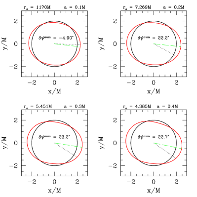
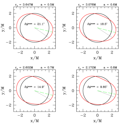
Figure 8: Embedding of distorted Kerr black hole event horizons for a corotating orbit — i.e., an orbit for which $\Omega_{\rm orb}=\Omega_{\rm H}$. As in Figs. 3, 5, and 6, the green dashed line points along the direction of greatest horizon distortion, and the black dotted line points to the orbiting body; the distortions are all scaled by a factor $\propto r_{\rm o}^{3}/\mu$. At very small spins (for which the corotating orbital radius is very large), the bulge lags the orbit slightly, but the bulge leads for all other spins.

Before concluding, let us examine the relative phase of the tidal field and the horizon’s curvature, Eq. (196). Setting $\delta\psi^{\rm TB}_{lm}=0$ yields

$$\Omega_{\rm orb}=\Omega_{\rm H}\,\frac{(l+2)(l-1)}{l(l+1)}\;.$$ (204)

We again see $\Omega_{\rm orb}\neq\Omega_{\rm H}$ when the field and the response are aligned (although $\Omega_{\rm orb}\to\Omega_{\rm H}$ as $l$ gets very large).

The analytical expansions and numerical data indicate that the Newtonian fluid intuition for the geometry of tidal coupling simply does not work well for strong-field black hole binaries, even accounting for the teleological swap of “lag” and “lead.” Only in the extremes can we make statements with confidence: when $\Omega_{\rm H}\gg\Omega_{\rm orb}$, the tidal bulge will lag the orbit; when $\Omega_{\rm orb}\gg\Omega_{\rm H}$, the bulge will lead the orbit. But when $\Omega_{\rm orb}$ and $\Omega_{\rm H}$ are of similar magnitude, we cannot make a clean prediction.

The tidal bulge is not locked to the orbit when $dE^{\rm H}/dt=0$, at least using any scheme to define the lead/lag angle that we have examined.

VI Conclusions

In this paper, we have presented a formalism for computing tidal distortions of Kerr black holes. Using black hole perturbation theory, our approach is good for fast motion, strong field orbits, and can be applied to a black hole of any spin parameter. We have also developed tools for visualizing the distorted horizon by embedding its 2-dimensional surface in a 3-dimensional Euclidean space. For now, our embeddings are only good for Kerr spin parameter $a/M\leq\sqrt{3}/2$, the highest value for which the entire horizon can be embedded in a globally Euclidean space. Higher spins require either a piecewise embedding of an equatorial “belt” in a Euclidean space, and a region near the “poles” in a Lorentzian space, or else embedding in a different space altogether.

Although our formalism is good for arbitrary bound orbits, we have focused on circular and equatorial orbits for this first analysis. This allowed us to validate this formalism against existing results in the literature, and to explore whether there is a simple connection between the tidal coupling of the hole to the orbit, and the relative geometry of the orbit and the horizon’s tidal bulge. We find that there is no such simple connection in general. Perhaps not surprisingly, strong-field black hole systems are more complicated than Newtonian fluid bodies.

We plan two followup analyses to extend the work we have done here. First, we plan to extend the work on embedding horizons to $a/M>\sqrt{3}/2$, the domain for which we cannot use a globally Euclidean embedding. Work in progress indicates that the simplest and perhaps most useful approach is to use the globally hyperbolic 3-space $H^{3}$ gibbons . This allows us to treat the entire range of physical black hole spins, $0\leq a/M\leq 1$, using a single global embedding space. Second, we plan to examine tidal distortions from generic — inclined and eccentric — Kerr orbits. The circular equatorial orbits we have studied in this first paper are stationary, as are the tidal fields and tidal responses that arise from them. If one examines the system and the horizon’s response in a frame that corotates with the orbit, the tide and the horizon will appear static. This will not be the case for generic orbits. Even when viewed in a frame that rotates at the orbit’s mean $\phi$ frequency, the orbit will be dynamical, and so the horizon’s response will likewise be dynamical. Similar analyses for Schwarzschild have already been presented by Vega, Poisson, and Massey vpm11 ; it will be interesting to compare with the more complicated and less symmetric Kerr case.

An extension of our analysis may be useful for improving initial data for numerical relativity simulations of merging binary black holes. One source of error in such simulations is that the black holes typically have the wrong initial geometry — unless the binary is extremely widely separated, we expect each hole to be distorted by their companion’s tides. Accounting for this in the initial data requires matching the near-horizon geometry to the binary’s spacetime metric; see chu14 for an up-to-date discussion of work to include tidal effects in a binary’s initial data. Much work has been done on binaries containing tidally deformed Schwarzschild black holes alvi ; yunesetal ; mcdanieletal , and efforts now focus on the more realistic case of binaries containing spinning black holes gallouinetal ; chu14 . With some effort (in order to get the geometry in a region near the horizon, not just on the horizon), we believe it should be possible to use this work as an additional tool for extending the matching procedure to the realistic orbital geometries of rotating black holes.

Appendix A Details of computing $\bar{\eth}$

In this appendix, we present details regarding the operator $\bar{\eth}$ in the form that we need it for our analysis.

A.1 The Newman-Penrose tetrad legs

A useful starting point is to write out the Newman-Penrose tetrad legs ${\bf l}$, ${\bf n}$, and ${\bf m}$. In much of the literature on black hole perturbation theory, we use the Kinnersley form of these tetrad legs in Boyer-Lindquist coordinates:

$$\left(l^{\mu}\right)_{\rm BL} \doteq \frac{1}{\Delta}\left[(r^{2}+a^{2}),\Delta,0,a\right]\;,$$ (205)

$$\left(n^{\mu}\right)_{\rm BL} \doteq \frac{1}{2\Sigma}\left[(r^{2}+a^{2}),-\Delta,0,a\right]\;,$$ (206)

$$\left(m^{\mu}\right)_{\rm BL} \doteq \frac{1}{\sqrt{2}(r+ia\cos\theta)}\left[ia\sin\theta,0,1,i\csc\theta\right]\;;$$ (207)

$$\left(l_{\mu}\right)_{\rm BL} \doteq \left[-1,\Sigma/\Delta,0,a\sin^{2}\theta\right]\;,$$ (208)

$$\left(n_{\mu}\right)_{\rm BL} \doteq \frac{1}{2\Sigma}\left[-\Delta,-\Sigma,0,a\Delta\sin^{2}\theta\right]\;,$$ (209)

$$\left(m_{\mu}\right)_{\rm BL} \doteq \frac{1}{\sqrt{2}(r+ia\cos\theta)}\left[-ia\sin\theta,0,\Sigma,i(r^{2}+a^{2})\sin\theta\right]\;.$$ (210)

The components of the fourth leg, ${\bf\bar{m}}$, are related to the components of ${\bf m}$ by complex conjugation. The notation $(b^{\mu})_{\rm BL}\doteq(b^{t},b^{r},b^{\theta},b^{\phi})$ means “the components of the 4-vector ${\bf b}$ in Boyer-Lindquist coordinates are represented by the array on the right-hand side,” and similarly for the 1-form components $(b_{\mu})_{\rm BL}$.

Because our analysis focuses on the Kerr black hole event horizon, we will find it useful to transform to Kerr ingoing coordinates $(v,r^{\prime},\theta,\psi)$. Using Eqs. (5) – (6), we transform tetrad components between the two coordinate systems with the matrix elements

$$\frac{\partial v}{\partial t}=1\;,\qquad\frac{\partial v}{\partial r}=\frac{r^{2}+a^{2}}{\Delta}\;,\qquad\frac{\partial\psi}{\partial r}=\frac{a}{\Delta}\;,\qquad\frac{\partial\psi}{\partial\phi}=1\;,\qquad\frac{\partial r^{\prime}}{\partial r}=1\;.$$ (211)

All elements which could connect $(t,r,\phi)$ and $(v,r^{\prime},\psi)$ which are not explicitly listed here are zero; the angle $\theta$ is the same in the two coordinate systems. The matrix elements for the inverse transformation are

$$\frac{\partial t}{\partial v}=1\;,\qquad\frac{\partial t}{\partial r^{\prime}}=-\frac{(r^{2}+a^{2})}{\Delta}\;,\qquad\frac{\partial\psi}{\partial r^{\prime}}=-\frac{a}{\Delta}\;,\qquad\frac{\partial\phi}{\partial\psi}=1\;,\qquad\frac{\partial r}{\partial r^{\prime}}=1\;.$$ (212)

As noted in the Introduction, $r$ and $r^{\prime}$ are identical; we just maintain a notational distinction for clarity while transforming between these two different coordinate systems.

With these, it is a simple matter to transform the tetrad components to their form in Kerr ingoing coordinates:

$$\left(l^{\mu}\right)_{\rm IN} \doteq \frac{1}{\Delta}\left[2[(r^{\prime})^{2}+a^{2}],\Delta,0,2a\right]\;,$$ (213)

$$\left(n^{\mu}\right)_{\rm IN} \doteq \frac{1}{2\Sigma}\left[0,-\Delta,0,0\right]\;,$$ (214)

$$\left(m^{\mu}\right)_{\rm IN} \doteq \frac{1}{\sqrt{2}(r^{\prime}+ia\cos\theta)}\left[ia\sin\theta,0,1,i\csc\theta\right]\;;$$ (215)

$$\left(l_{\mu}\right)_{\rm IN} \doteq \left[-1,2\Sigma/\Delta,0,a\sin^{2}\theta\right]\;,$$ (216)

$$\left(n_{\mu}\right)_{\rm IN} \doteq \frac{1}{2\Sigma}\left[-\Delta,0,0,a\Delta\sin^{2}\theta\right]\;,$$ (217)

$$\left(m_{\mu}\right)_{\rm IN} \doteq \frac{1}{\sqrt{2}(r^{\prime}+ia\cos\theta)}\left[-ia\sin\theta,0,\Sigma,i[(r^{\prime})^{2}+a^{2})\sin\theta\right]\;.$$ (218)

The notation $(b^{\mu})_{\rm IN}\doteq(b^{v},b^{r^{\prime}},b^{\theta},b^{\psi})$ means “the components of the 4-vector ${\bf b}$ in Kerr ingoing coordinates are represented by the array on the right-hand side,” and similarly for the 1-form components $(b_{\mu})_{\rm IN}$. In the above equations, $\Delta$ and $\Sigma$ take their usual forms, but with $r\to r^{\prime}$. At this point, the notational distinction between $r^{\prime}$ and $r$ is no longer needed, so we drop the prime on $r$ in what follows.

Changing coordinates is not enough to fix various pathologies associated with the behavior of quantities on the event horizon. To ensure that quantities we examine are well behaved there, we next change to the Hawking-Hartle tetrad. This is done in two steps. First we perform a boost (cf. Ref. stewart , Sec. 2.6), putting

$${\bf l^{\prime}} = \frac{\Delta}{2\varpi^{2}}\,{\bf l}\;,$$ (219)

$${\bf n^{\prime}} = \frac{2\varpi^{2}}{\Delta}\,{\bf n}\;,$$ (220)

$${\bf m^{\prime}} = {\bf m}\;,$$ (221)

where we’ve introduced $\varpi^{2}=r^{2}+a^{2}$. This is followed by a null rotation around ${\bf l}$:

$${\bf l}_{\rm HH} = {\bf l^{\prime}}\;,$$ (222)

$${\bf m}_{\rm HH} = {\bf m^{\prime}}+\bar{c}\,{\bf l^{\prime}}\;,$$ (223)

$${\bf n}_{\rm HH} = {\bf n^{\prime}}+c\,{\bf m^{\prime}}+\bar{c}\,{\bf\bar{m}^{\prime}}+c\bar{c}\,{\bf l^{\prime}}\;,$$ (224)

with

$$c=\frac{ia\sin\theta}{\sqrt{2}(r-ia\cos\theta)}\;.$$ (225)

With this, we finally obtain the tetrad elements that we need for this analysis:

$$\left(l^{\mu}\right)_{\rm HH,\,IN} \doteq \frac{1}{\varpi^{2}}\left[\varpi^{2},\Delta/2,0,a\right]\;,$$ (226)

$$\left(m^{\mu}\right)_{\rm HH,\,IN} \doteq \frac{1}{\sqrt{2}(r+ia\cos\theta)}\left[0,-\frac{ia\Delta\sin\theta}{2\varpi^{2}},1,i\csc\theta-\frac{ia^{2}\sin\theta}{\varpi^{2}}\right]\;,$$ (227)

$$\left(n^{\mu}\right)_{\rm HH,\,IN} \doteq \frac{1}{4\varpi^{2}\Sigma}\left[-2a^{2}\varpi^{2}\sin^{2}\theta,-4\varpi^{4}+a^{2}\Delta\sin^{2}\theta,0,-4a\varpi^{2}+2a^{3}\sin^{2}\theta\right]\;;$$ (228)

$$\left(l_{\mu}\right)_{\rm HH,\,IN} \doteq \frac{1}{2\varpi^{2}}\left[-\Delta,2\Sigma,0,a\Delta\sin^{2}\theta\right]\;,$$ (229)

$$\left(m_{\mu}\right)_{\rm HH,\,IN} \doteq \frac{1}{\sqrt{2}(r+ia\cos\theta)}\times\frac{1}{2(r^{2}+a^{2})}\times$$ (230)

$$\left[-ia(2\varpi^{2}-\Delta)\sin\theta,-2ia\Sigma\sin\theta,2\varpi^{2}\Sigma,i\left(2\varpi^{4}-a^{2}\Delta\sin^{2}\theta\right)\sin\theta\right]\;,$$

$$\left(n_{\mu}\right)_{\rm HH,\,IN} \doteq \frac{1}{4\varpi^{2}\Sigma}\left[-4\varpi^{4}+a^{2}\left(4\varpi^{2}-\Delta\right)\sin^{2}\theta,2a^{2}\Sigma\sin^{2}\theta,0,a^{3}\Delta\sin^{4}\theta\right]\;.$$ (231)

In the remainder of this appendix, we will use the Hawking-Hartle components in ingoing coordinates, and will drop the “HH, IN” subscript.

A.2 Constructing $\bar{\eth}$

Here we derive the form of the operator $\bar{\eth}$, acting at the radius of the Kerr event horizon, $r=r_{+}$. Following Hartle hartle74 , $\bar{\eth}$ acting upon a quantity $\eta$ of spin-weight $s$ is given by

$$\bar{\eth}\eta=\left[\bar{\delta}-s(\alpha-\bar{\beta})\right]\eta\;.$$ (232)

The operator $\bar{\delta}=\bar{m}^{\mu}\partial_{\mu}$. Evaluating this at $r=r_{+}$ [using the fact that $\Delta=0$ there, and that $a/(r_{+}^{2}+a^{2})=a/(2Mr_{+})=\Omega_{\rm H}$] we find

$$\bar{\delta}=\frac{1}{\sqrt{2}(r_{+}-ia\cos\theta)}\left[\partial_{\theta}-i(\csc\theta-a\Omega_{\rm H}\sin\theta)\partial_{\psi}\right]\;.$$ (233)

Next consider the Newman-Penrose spin coefficients $\alpha$ and $\beta$. With the metric signature we use ($-+++$), they are given by

$$\alpha = \frac{1}{2}\bar{m}^{\nu}\left(\bar{m}^{\mu}\nabla_{\nu}m_{\mu}-n^{\mu}\nabla_{\nu}l_{\mu}\right)\;,$$ (234)

$$\beta = \frac{1}{2}m^{\nu}\left(\bar{m}^{\mu}\nabla_{\nu}m_{\mu}-n^{\mu}\nabla_{\nu}l_{\mu}\right)\;.$$ (235)

This means that

$$\alpha-\bar{\beta}=\frac{1}{2}\bar{m}^{\nu}\left(\bar{m}^{\mu}\nabla_{\nu}m_{\mu}-m^{\mu}\nabla_{\nu}\bar{m}_{\mu}\right)\;.$$ (236)

Using ingoing coordinates, we find

$$\left(\alpha-\bar{\beta}\right)|_{r\to r_{+}} = \frac{(a^{2}-2Mr_{+})\cot\theta+iar_{+}\csc\theta}{\sqrt{2}r_{+}(r_{+}-ia\cos\theta)^{2}}$$ (237)

$$= \frac{1}{\sqrt{2}(r_{+}-ia\cos\theta)^{2}}\left[\frac{(a^{2}-2Mr_{+})}{r_{+}}\cot\theta+ia\csc\theta\right]\;.$$

Finally, we combine Eqs. (233) and (237) to build $\bar{\eth}$. Assume that $\eta$ is a function of spin-weight $s$ with an axial dependence $e^{im\psi}$:

$$\bar{\eth}\eta = \frac{1}{\sqrt{2}(r_{+}-ia\cos\theta)}\left[\partial_{\theta}-i(\csc\theta-a\Omega_{\rm H}\sin\theta)\partial_{\psi}-\frac{s}{(r_{+}-ia\cos\theta)}\left[\frac{(a^{2}-2Mr_{+})}{r_{+}}\cot\theta+ia\csc\theta\right]\right]\eta$$ (238)

$$= \frac{1}{\sqrt{2}(r_{+}-ia\cos\theta)}\biggl{[}\partial_{\theta}+s\cot\theta+m\csc\theta-am\Omega_{\rm H}\sin\theta$$

$$\qquad\qquad\qquad\qquad\left.-s\cot\theta-\frac{s}{(r_{+}-ia\cos\theta)}\left[\frac{(a^{2}-2Mr_{+})}{r_{+}}\cot\theta+ia\csc\theta\right]\right]\eta$$

$$= \frac{1}{\sqrt{2}(r_{+}-ia\cos\theta)}\left[L^{s}_{-}-am\Omega_{\rm H}\sin\theta-\frac{s}{(r_{+}-ia\cos\theta)}\left[\frac{(a^{2}+r_{+}^{2}-2Mr_{+}-iar_{+}\cos\theta)\cot\theta}{r_{+}}+ia\csc\theta\right]\right]\eta$$

$$= \frac{1}{\sqrt{2}(r_{+}-ia\cos\theta)}\left[L^{s}_{-}-am\Omega_{\rm H}\sin\theta-\frac{s}{(r_{+}-ia\cos\theta)}\left(ia\csc\theta-ia\cos\theta\cot\theta\right)\right]\eta$$

$$= \frac{1}{\sqrt{2}(r_{+}-ia\cos\theta)}\left[L^{s}_{-}-am\Omega_{\rm H}\sin\theta-\frac{ias\sin\theta}{(r_{+}-ia\cos\theta)}\right]\eta$$

$$= \frac{1}{\sqrt{2}r_{+}}\left(1-\frac{ia\cos\theta}{r_{+}}\right)^{s-1}\left[L^{s}_{-}-am\Omega_{\rm H}\sin\theta\right]\left(1-\frac{ia\cos\theta}{r_{+}}\right)^{-s}\eta$$

In going from the first to the second equality in Eq. (238), we used the fact that $\eta\propto e^{im\psi}$; we also added and subtracted $s\cot\theta$ inside the square brackets. In going from the second to the third equality, we recognized that the first three terms inside the brackets are just the operator $L^{s}_{-}$; cf. Eq. (63). We also moved the negative $s\cot\theta$ term inside the second set of square brackets. In going from the third to the fourth equality, we used the fact that $r_{+}^{2}+a^{2}=2Mr_{+}$. We then used $\csc\theta-\cot\theta\cos\theta=\sin\theta$ to go from the fourth to the fifth, and finally used Eq. (LABEL:eq:usefulidentity) to obtain our final form for this operator. This last line is identical to Eq. (LABEL:eq:kerr_eth).

Appendix B Visualizing a distorted horizon

Following Hartle hartle73 ; hartle74 , we visualize distorted horizons by embedding the two-surface of the horizon on a constant time surface in a flat three-dimensional space. The embedding is a surface $r_{\rm E}(\theta,\psi)$ that has the same Ricci scalar curvature as the distorted horizon. For unperturbed Schwarzschild black holes, $r_{\rm E}=2M$; for an unperturbed Kerr hole, $r_{\rm E}$ is a more complicated function that varies with $\theta$. In the general case, we write

$$r_{\rm E}(\theta,\psi)=r_{\rm E}^{(0)}(\theta)+r_{\rm E}^{(1)}(\theta,\psi)\;.$$ (239)

In this paper, we focus on cases where the entire horizon can be embedded in a Euclidean space, which means that we require $a/M\leq\sqrt{3}/2$. (We briefly discuss considerations for $a/M>\sqrt{3}/2$ at the end of this appendix.) To generate the embedding, we define Cartesian coordinates on the horizon as usual:

$$X(\theta,\psi) = r_{\rm E}(\theta,\psi)\sin\theta\cos\psi\;,$$ (240)

$$Y(\theta,\psi) = r_{\rm E}(\theta,\psi)\sin\theta\sin\psi\;,$$ (241)

$$Z(\theta,\psi) = r_{\rm E}(\theta,\psi)\cos\theta\;.$$ (242)

We compute the line element

$$ds^{2} = dX^{2}+dY^{2}+dZ^{2}$$ (243)

$$\equiv g^{\rm E}_{\theta\theta}d\theta^{2}+2g^{\rm E}_{\theta\psi}d\theta\,d\psi+g^{\rm E}_{\psi\psi}d\psi^{2}\;,$$

and then the Ricci scalar corresponding to the embedding metric $g^{\rm E}_{\alpha\beta}$ to linear order in $r_{\rm E}^{(1)}$. We require this to equal the scalar curvature computed using Eq. (LABEL:eq:gauss_kerr), and then read off the distortion $r_{\rm E}^{(1)}(\theta,\psi)$.

B.1 Schwarzschild

Thanks to the spherical symmetry of the undistorted Schwarzschild black hole, results for this limit are quite simple. The metric on an embedded surface of radius

$$r_{\rm E}=2M+r_{\rm E}^{(1)}(\theta,\phi)$$ (244)

is given by

$$ds^{2}=(2M)^{2}\left[1+\frac{r_{\rm E}^{(1)}(\theta,\phi)}{M}\right](d\theta^{2}+\sin^{2}\theta\,d\phi^{2})\;.$$ (245)

(Recall that $\psi=\phi$ for $a=0$.) It is a straightforward exercise to compute the scalar curvature associated with the metric (245); we find

$$R_{\rm E}=\frac{1}{2M^{2}}-\left[2+\frac{1}{\sin\theta}\frac{\partial}{\partial\theta}\left(\sin\theta\frac{\partial}{\partial\theta}\right)-\frac{m^{2}}{\sin^{2}\theta}\right]\frac{r_{\rm E}^{(1)}}{4M^{3}}\;.$$ (246)

Let us expand $r_{\rm E}^{(1)}$ in spherical harmonics:

$$r_{\rm E}^{(1)}(\theta,\phi)=2M\sum_{lm}\varepsilon_{lm}\,{{}_{0}}Y_{lm}(\theta)e^{im\phi}\;.$$ (247)

Using this, Eq. (246) simplifies further:

$$R_{\rm E}=\frac{1}{2M^{2}}\left[1+\sum_{lm}\varepsilon_{lm}(l+2)(l-1){{}_{0}}Y_{lm}(\theta)e^{im\phi}\right]\;.$$ (248)

The scalar curvature we compute using black hole perturbation theory takes the form

$$R_{\rm H}=R^{(0)}_{\rm H}+\sum_{lmkn}R^{(1)}_{{\rm H},lmkn}\;,$$ (249)

where $R^{(0)}_{\rm H}=1/2M^{2}$. Equating this to $R_{\rm E}$, we find

$$\varepsilon_{lm}\,{{}_{0}}Y_{lm}(\theta)e^{im\phi}=\sum_{kn}\frac{2M^{2}R^{(1)}_{{\rm H},lmkn}}{(l+2)(l-1)}\;,$$ (250)

or

$$r_{\rm E}^{(1)}(\theta,\phi)=\sum_{lmkn}\frac{4M^{3}R^{(1)}_{{\rm H},lmkn}}{(l+2)(l-1)}\;.$$ (251)

Equation (251) is identical (modulo a slight change in notation) to the embedding found in Ref. vpm11 ; compare their Eqs. (4.33) and (4.34). We use $r_{\rm E}^{(1)}(\theta,\phi)$ to visualize distorted Schwarzschild black holes in Sec. III.2 (dropping the indices $k$ and $n$ since we only present results for circular, equatorial orbits in this paper).

B.2 Kerr

Embedding a distorted Kerr black hole is rather more complicated. Indeed, embedding an undistorted Kerr black hole is not trivial: as discussed in Sec. II.1, the scalar curvature $R_{\rm H}$ of an undistorted Kerr black hole changes sign near the poles for spins $a/M>\sqrt{3}/2$. A hole with this spin cannot be embedded in a global Euclidean space, and one must instead use a Lorentzian embedding near the poles smarr . We briefly describe how to embed a tidally distorted black hole with $a/M>\sqrt{3}/2$ at the end of this appendix, but defer all details to a later paper. For now, we focus on the comparatively simple case $a/M\leq\sqrt{3}/2$.

B.2.1 Undistorted Kerr

We begin by reviewing embeddings of the undistorted case. Working in ingoing coordinates, the metric on the horizon is given by

$$ds^{2}=g_{xx}\,dx^{2}+g_{\psi\psi}\,d\psi^{2}\;,\qquad{\rm with}$$

$$g_{xx}=\frac{r_{+}^{2}+a^{2}x^{2}}{1-x^{2}}\;,\quad g_{\psi\psi}=\frac{4M^{2}r_{+}^{2}(1-x^{2})}{r_{+}^{2}+a^{2}x}\;.$$

(252)

We have introduced $x\equiv\cos\theta$. Equation (252) is the metric on a spheroid of radius

$$r^{(0)}(x)=\sqrt{r_{\perp}(x)^{2}+Z(x)^{2}}\;,$$ (253)

where

$$r_{\perp}(x) = \eta\sqrt{f(x)}\;,$$ (254)

$$Z(x) = \eta\int_{0}^{x}\sqrt{\frac{4-(df/dx)^{2}}{4f(x^{\prime})}}dx^{\prime}\;,$$ (255)

with

$$f(x) = \frac{1-x^{2}}{1-\beta^{2}(1-x^{2})}\;,$$ (256)

$$\eta = \sqrt{r_{+}^{2}+a^{2}}\;,$$ (257)

$$\beta = a/\eta\;.$$ (258)

Using Eqs. (256) – (258), we can rewrite $Z(x)$ as

$$Z(x)=\int_{0}^{x}\frac{H(x^{\prime})}{\left[r_{+}^{2}+a^{2}(x^{\prime})^{2}\right]^{3/2}}dx^{\prime}\;,$$ (259)

where

$$H(x) = \bigl{[}r_{+}^{8}-6a^{4}r_{+}^{4}x^{2}-4a^{6}r_{+}^{2}x^{2}(1+x^{2})$$ (260)

$$\qquad-a^{8}x^{2}(1+x^{2}+x^{4})\bigr{]}^{1/2}\;.$$

For $a/M>\sqrt{3}/2$, $H(x)=0$ at some value $|x|=x_{\rm E}$. This means that $H(x)$ is imaginary for $|x|>x_{\rm E}$ for this spin; $Z$ is imaginary over this range as well. The horizon can be embedded in a Euclidean space over the range $-x_{\rm E}\leq x\leq x_{\rm E}$. For all $a$, the equator ($x=0$) is a circle of radius $2M$. The scalar curvature associated with this metric is

$$R^{(0)}_{\rm E}=R^{(0)}_{\rm H}=\frac{2}{r_{+}^{2}}\frac{(1+a^{2}/r_{+}^{2})(1-3a^{2}x^{2}/r_{+}^{2})}{(1+a^{2}x^{2}/r_{+}^{2})^{3}}\;.$$ (261)

B.2.2 Distorted Kerr: $a/M\leq\sqrt{3}/2$

For this calculation, it will be convenient to use Dirac notation to describe the dependence on $x$. We write the spin-weighted spherical harmonics as a ket,

$${{}_{s}}Y_{lm}(x)\longrightarrow|slm\rangle\;,$$ (262)

and define the inner product

$$\langle skm|f(x)|slm\rangle=2\pi\int_{-1}^{1}{{}_{s}}Y_{km}(x)f(x){{}_{s}}Y_{lm}(x)dx\;.$$ (263)

These harmonics are normalized so that

$$\delta_{kl}\delta_{nm} = \int_{0}^{2\pi}d\psi\int_{-1}^{1}dx\,{{}_{s}}Y_{kn}(x){{}_{s}}Y_{lm}(x)e^{i(m-n)\psi}$$ (264)

$$\equiv \delta_{nm}\langle skn|slm\rangle\;.$$

The $2\pi$ prefactor in Eq. (263) means that

$$\langle skm|slm\rangle=\delta_{kl}\;.$$ (265)

Using this notation, let us now consider the curvature of a tidally distorted Kerr black hole. Begin with the curvature from black hole perturbation theory, Eq. (LABEL:eq:gauss_kerr). Translating into Dirac notation, we have

$$|R^{(1)}_{\rm H}\rangle = {\rm Im}\sum_{lmkn}\left[{\cal C}_{lmkn}Z^{\rm H}_{lmkn}e^{i\Phi_{mkn}}|\bar{\eth}\bar{\eth}S^{+}_{lmkn}\rangle\right]$$ (266)

$$\equiv {\rm Im}\,R^{(1)}_{\rm H,c}\;,$$

where $|\bar{\eth}\bar{\eth}S^{+}_{lmkn}\rangle$ is given by Eq. (LABEL:eq:barethbarethS).

We now must assume a functional form for the embedding surface. A key issue is what basis functions we should use to describe the angular dependence of this surface. The basis functions for the angular sector, $\bar{\eth}\bar{\eth}S^{+}_{lmkn}$, depend on mode frequency, and so are not useful for describing the embedding surface. Since spherical harmonics are complete functions on the sphere, we use

$$r_{\rm E}(x,\psi)=r_{\rm E}^{0}(x)+r_{\rm E}^{(1)}(x,\psi)\;,$$ (267)

where

$$r_{\rm E}^{(1)}(x,\psi)=r_{+}\sum_{\ell m}\varepsilon_{\ell m}\,{{}_{0}}Y_{\ell m}(x)e^{im\psi}\;,$$ (268)

and where $r_{\rm E}^{0}(\theta)$ is given by Eq. (253). This quantity must be real, so the expansion coefficients must satisfy the symmetry

$$\varepsilon_{\ell-m}=(-1)^{\ell}\bar{\varepsilon}_{\ell m}\;,$$ (269)

where as before overbar denotes complex conjugate. Note that the index $\ell$ used in Eq. (268) is not the same as the index $l$ used in Eq. (266). It is important to maintain a distinction between the indices that are used on the spheroidal and the spherical harmonics.

Using Eqs. (267) and (268), we find that the embedding surface yields a metric on the horizon given by

$$ds^{2}=(g_{xx}+h_{xx})dx^{2}+2h_{x\psi}\,dx\,d\psi+(g_{\psi\psi}+h_{\psi\psi})d\psi^{2}\;,$$ (270)

with $g_{xx}$ and $g_{\psi\psi}$ given by Eq. (252), and

$$h_{xx} = \frac{2}{(r_{+}^{2}+a^{2}x^{2})^{3/2}}\left[\left(H+\frac{4M^{2}r_{+}^{2}x^{2}}{1-x^{2}}\right)r^{(1)}+\left(H-4M^{2}r_{+}^{2}\right)x\frac{\partial r^{(1)}}{\partial x}\right]\;,$$ (271)

$$h_{x\psi} = \frac{(H-4M^{2}r_{+}^{2})x}{(r_{+}^{2}+a^{2}x^{2})^{3/2}}\frac{\partial r^{(1)}}{\partial\psi}\;,$$ (272)

$$h_{\psi\psi} = 4\frac{Mr_{+}(1-x^{2})}{\sqrt{r_{+}^{2}+a^{2}x^{2}}}\,r^{(1)}\;.$$ (273)

The function $H=H(x)$ was introduced in the embedding of the undistorted Kerr hole, Eq. (260). By restricting ourselves to $a/M\leq\sqrt{3}/2$, we are guaranteed that $H$ is real for this analysis.

Computing the embedding curvature from this metric, we find

$$R_{\rm E}=R^{(0)}_{\rm E}+R^{(1)}_{\rm E}\;,$$ (274)

where $R^{(0)}_{\rm E}$ is given by Eq. (261), and

$$R^{(1)}_{\rm E}\longrightarrow|R^{(1)}_{\rm E}\rangle = \sum_{\ell m}\varepsilon_{\ell m}\left[C(x)|0\ell m\rangle+D(x)\,\frac{d}{dx}|0\ell m\rangle\right]e^{im\psi}$$ (275)

$$\equiv \sum_{\ell m}\varepsilon_{\ell m}e^{im\psi}{\cal E}|0\ell m\rangle\;.$$

We’ve introduced the operator ${\cal E}=C(x)+D(x)\,d/dx$ for later notational convenience. The functions $C(x)$ and $D(x)$ which appear in it are given by

$$C(x) = \frac{1}{2HM^{2}r_{+}(r_{+}^{2}+a^{2}x^{2})^{11/2}}\left[\sum_{j=0}^{8}c_{0,j}\,a^{2j}+\sum_{j=0}^{5}\frac{c_{1,j}\,a^{2j}}{1-x^{2}}\right]\;,$$ (276)

$$D(x) = \frac{1}{HM(r_{+}^{2}+a^{2}x^{2})^{11/2}}\sum_{j=0}^{7}d_{j}\,a^{2j}\;,$$ (277)

where

$$c_{0,0} = 2r_{+}^{5}\left\{\ell(\ell+1)HM\left[r_{+}^{6}+4M^{2}(H-4M^{2}r_{+}^{2})x^{2}\right]-r_{+}^{11}+2r_{+}^{5}(r_{+}^{6}-4HM^{2})x^{2}\right\}\;,$$ (278)

$$c_{0,1} = 8\ell(\ell+1)H^{2}M^{3}r_{+}^{3}x^{4}-r_{+}^{14}(6-23x^{2}+9x^{4})$$ (279)

$$\quad-2HMr_{+}^{5}\left\{16\ell(\ell+1)M^{4}x^{4}+6Mr_{+}^{3}x^{2}(4-3x^{2})+r_{+}^{4}\left[1-(4+5\ell(\ell+1))x^{2}\right]\right\}\;,$$

$$c_{0,2} = r_{+}^{6}\left\{4\left[6+5\ell(\ell+1)\right]HMr_{+}x^{4}-12HM^{2}x^{2}(4-9x^{2})-r_{+}^{6}(6-63x^{2}+57x^{4})\right\}\;,$$ (280)

$$c_{0,3} = r_{+}^{4}\left\{4HMr_{+}x^{4}\left[3+\left[6+5\ell(\ell+1)\right]x^{2}\right]-4HM^{2}x^{2}(4-27x^{2})-r_{+}^{6}(2-103x^{2}+181x^{4}-24x^{6})\right\}\;,$$ (281)

$$c_{0,4} = r_{+}^{2}x^{2}\left\{36HM^{2}x^{2}+2HMr_{+}x^{4}\left[8+\left[4+5\ell(\ell+1)\right]x^{2}\right]+r_{+}^{6}(104-332x^{2}+67x^{4}+21x^{6})\right\}\;,$$ (282)

$$c_{0,5} = r_{+}x^{2}\left\{2HMx^{6}\left[3+\ell(\ell+1)x^{2}\right]+r_{+}^{5}(63-355x^{2}+56x^{4}+62x^{6}+6x^{8})\right\}\;,$$ (283)

$$c_{0,6} = r_{+}^{4}x^{2}(21-217x^{2}+6x^{4}+60x^{6}+18x^{8})\;,$$ (284)

$$c_{0,7} = r_{+}^{2}x^{2}(3-71x^{2}-8x^{4}+18x^{6}+18x^{8})\;,$$ (285)

$$c_{0,8} = -x^{4}(10+x^{2}+x^{4}-6x^{6})\;;$$ (286)

$$c_{1,0} = 2m^{2}Mr_{+}^{3}(2HMr_{+}^{7}-Hr_{+}^{8}-4H^{2}M^{2}r_{+}^{2}x^{2}+16HM^{4}r_{+}^{4}x^{2}-2HMr_{+}^{7}x^{2}+8M^{3}r_{+}^{9}x^{2})\;,$$ (287)

$$c_{1,1} = -2Hm^{2}Mr_{+}^{3}x^{2}\left[5r_{+}^{6}+4M^{2}(H-4M^{2}r_{+}^{2})x^{2}\right]\;,$$ (288)

$$c_{1,2} = -4m^{2}Mr_{+}^{6}x^{4}\left[H(6M+5r_{+})-6M(H-4M^{2}r_{+}^{2})x^{2}\right]\;,$$ (289)

$$c_{1,3} = -4m^{2}Mr_{+}^{4}x^{6}\left[H(8M+5r_{+})-8M(H-4M^{2}r_{+}^{2})x^{2}\right]\;,$$ (290)

$$c_{1,4} = -2m^{2}Mr_{+}^{2}x^{8}\left[H(6M+5r_{+})-6M(H-4M^{2}r_{+}^{2})x^{2}\right]\;,$$ (291)

$$c_{1,5} = -2Hm^{2}Mr_{+}x^{10}\;;$$ (292)

$$d_{0} = 2r_{+}^{8}x\left\{-2r_{+}^{6}(1-x^{2})+HM\left[r_{+}+M(6-8x^{2})\right]\right\}\;,$$ (293)

$$d_{1} = r_{+}^{6}x\left\{-r_{+}^{6}(8-17x^{2}+9x^{4})+4HM\left[6M-2(9M-r_{+})x^{2}+9Mx^{4}\right]\right\}\;,$$ (294)

$$d_{2} = -4r_{+}^{4}x\left\{r_{+}^{6}(1-13x^{2}+12x^{4})-3HM\left[M-8Mx^{2}+(6M+r_{+})x^{4}\right]\right\}\;,$$ (295)

$$d_{3} = r_{+}^{2}x^{3}\left\{r_{+}^{6}(89-113x^{2}+24x^{4})+4HM\left[2r_{+}x^{4}-M(10-9x^{2})\right]\right\}\;,$$ (296)

$$d_{4} = 2HMr_{+}x^{9}+r_{+}^{6}x^{3}(75-149x^{2}+53x^{4}+21x^{6})\;,$$ (297)

$$d_{5} = r_{+}^{4}x^{3}(30-114x^{2}+35x^{4}+43x^{6}+6x^{8})\;,$$ (298)

$$d_{6} = r_{+}^{2}x^{3}(5-47x^{2}+7x^{4}+23x^{6}+12x^{8})\;,$$ (299)

$$d_{7} = -x^{5}(8-x^{2}-x^{4}-6x^{6})\;.$$ (300)

The term in $C(x)$ that is proportional to $1/(1-x^{2})$ is written so that $C(x)$ is well behaved in the limit $x\to\pm 1$:

$$\lim_{x\to\pm 1}\sum_{j=0}^{5}\frac{c_{1,j}\,a^{2j}}{1-x^{2}}=128a^{2}m^{2}M^{6}\biggl{[}64M^{7}r_{+}-16a^{2}M^{5}(3r_{+}+2M)-8a^{4}M^{3}(r_{+}-2M)+a^{6}M(5r_{+}+6M)-a^{8}\biggr{]}\;.$$

This ensures that this function is well-behaved in all of our numerical applications.

For small spin, the functions $C$ and $D$ become

$$C(x) = \frac{(\ell+2)(\ell-1)}{2M^{2}}+\frac{\ell(\ell+1)(5x^{2}-2)+2(18x^{2}+m^{2}-7)}{16M^{2}}\left(\frac{a}{M}\right)^{2}$$ (302)

$$-\frac{498x^{4}-764x^{2}+168-4m^{2}(5x^{2}+6)-\ell(\ell+1)(51x^{4}-100x^{2}+16)}{256M^{2}}\left(\frac{a}{M}\right)^{4}+\ldots$$

$$D(x) = \frac{5x(1-x^{2})}{8M^{2}}\left(\frac{a}{M}\right)^{2}+\frac{x(1-x^{2})(58-67x^{2})}{64M^{2}}\left(\frac{a}{M}\right)^{4}+\ldots\;.$$ (303)

The two expressions for the deformed hole’s curvature, Eqs. (266) and (275), must equal one another. To facilitate comparing the two expressions, let us introduce a complex embedding curvature, $R^{(1)}_{{\rm E,c}}$. In Dirac notation, we write this quantity

$$|R^{(1)}_{\rm E,c}\rangle=\sum_{\ell m}\varepsilon^{\rm c}_{\ell m}e^{im\psi}{\cal E}|0\ell m\rangle\;,$$ (304)

introducing new coefficients $\varepsilon^{\rm c}_{\ell m}$. We require that

$${\rm Im}\,R^{(1)}_{\rm E,c}=R^{(1)}_{\rm E}\;.$$ (305)

Referring to Eq. (266), we see that we can enforce $R^{(1)}_{\rm E}=R^{(1)}_{\rm H}$ by requiring

$$R^{(1)}_{\rm E,c}=R^{(1)}_{\rm H,c}\;.$$ (306)

As we will now show, Eq. (306) gives us a simple expression for the complex embedding coefficients $\varepsilon_{\ell m}^{\rm c}$. Once those coefficients are known, it is straightforward to extract the embedding coefficients $\varepsilon_{\ell m}$.

Both $R^{(1)}_{\rm E,c}$ and $R^{(1)}_{\rm H,c}$ vary with $\psi$ as $e^{im\psi}$, so we can examine them $m$-mode by $m$-mode. To facilitate this comparison, we break up the phase function $\Phi_{mkn}(v,\psi)$ [Eq. (29)] as

$$\Phi_{mkn}(v,\psi)=m\psi+\delta\Phi_{m}+\delta\Phi_{kn}\;,$$ (307)

with

$$\delta\Phi_{m} = -m\left[\Omega_{\phi}v+K(a)\right]\;,$$

$$\delta\Phi_{kn} = -(k\Omega_{\theta}+n\Omega_{r})v\;.$$ (308)

Recall $K(a)$ is defined in Eq. (LABEL:eq:K_of_a).

With all of this in hand, let us now compare the two curvature expressions for each $m$:

$$|{{}_{m}R}^{(1)}_{\rm H,c}\rangle = e^{i\delta\Phi_{m}}\sum_{lkn}{\cal C}_{lmkn}Z^{\rm H}_{lmkn}e^{i\delta\Phi_{kn}}|\bar{\eth}\bar{\eth}S^{+}_{lmkn}\rangle\;,$$

$$|{{}_{m}R}^{(1)}_{\rm E,c}\rangle = \sum_{\ell}\varepsilon^{\rm c}_{\ell m}{\cal E}|0\ell m\rangle\;.$$ (309)

The sums over $l$ and $\ell$ are taken from ${\rm min}(2,|m|)$ to $\infty$; the sums over $k$ and $n$ are both taken from $-\infty$ to $\infty$. Multiply these expressions by $e^{im\psi}$ and sum over $m$ from $-\infty$ to $\infty$ to recover our expressions for $R^{(1)}_{\rm E,c}$ and $R^{(1)}_{\rm H,c}$.

Left multiply both expressions in Eq. (309) by $\langle 0qm|$. Define the vector ${{}_{m}}\vec{R}^{\rm c}$ as the object with components

$${{}_{m}}R^{\rm c}_{q}=e^{i\delta\Phi_{m}}\sum_{lkn}{\cal C}_{lmkn}Z^{\rm H}_{lmkn}e^{i\delta\Phi_{kn}}\langle 0qm|\bar{\eth}\bar{\eth}S^{+}_{lmkn}\rangle\;.$$ (310)

Likewise define the embedding matrix ${{}_{m}}\mathsf{E}$ as the object whose components are

$${{}_{m}}\mathsf{E}_{q\ell}=\langle 0qm|{\cal E}|0\ell m\rangle\;.$$ (311)

The function $C(x)$ which appears in the operator ${\cal E}$ is an even function of $x$, and $D(x)$ [which appears in ${\cal E}$ in the combination $D(x)\,d/dx$] is odd. It follows that the only non-zero elements of ${{}_{m}}\mathsf{E}_{q\ell}$ are those for which $q$ and $\ell$ are either both even or both odd.

Finally, define ${{}_{m}}\vec{\boldsymbol{\varepsilon}}^{\rm c}$ as the vector whose components are $\varepsilon^{\rm c}_{\ell m}$. Requiring $\langle 0qm|{{}_{m}}R^{(1)}_{\rm H,c}\rangle=\langle 0qm|{{}_{m}}R^{(1)}_{\rm E,c}\rangle$ yields the matrix equation

$${{}_{m}}{\vec{R}}^{\rm c}={{}_{m}}\mathsf{E}\cdot{{}_{m}}\vec{\boldsymbol{\varepsilon}}^{\rm c}\;,$$ (312)

which is easily solved:

$${{}_{m}}\vec{\boldsymbol{\varepsilon}}^{\rm c}={{}_{m}}\mathsf{E}^{-1}\cdot{{}_{m}}{\vec{R}}^{\rm c}\;.$$ (313)

Equation (313) yields the complex embedding coefficients $\varepsilon^{\rm c}_{\ell m}$. From this, we must extract the true embedding coefficients $\varepsilon_{\ell m}$ which appear in Eq. (268). We do this by considering the symmetries of $\varepsilon^{\rm c}_{\ell m}$ and $\varepsilon_{\ell m}$, and by enforcing Eq. (305). We have already presented the symmetry of $\epsilon_{\ell m}$ in Eq. (269). For $\varepsilon^{\rm c}_{\ell m}$, first write Eq. (313) in index notation,

$$\varepsilon^{\rm c}_{\ell m}=\sum_{q}{{}_{m}}\mathsf{E}^{-1}_{\ell q}\,\,{{}_{m}}R^{\rm c}_{q}\;.$$ (314)

Carefully examining their definitions and the symmetries of the quantities which go into them, we find that

$${{}_{-m}}\mathsf{E}_{q\ell} = (-1)^{\ell}\,\,{{}_{m}}\mathsf{E}_{q\ell}\;,$$

$${{}_{-m}}R^{\rm c}_{q} = -({{}_{m}}\bar{R}^{\rm c}_{q})\;,$$ (315)

so

$$\varepsilon^{\rm c}_{\ell-m}=(-1)^{\ell+1}\bar{\varepsilon}^{\rm c}_{\ell m}\;.$$ (316)

Now enforce Eq. (305): We require

$${\rm Im}\sum_{\ell m}\varepsilon^{\rm c}_{\ell m}\,e^{im\psi}{\cal E}{{}_{0}}Y_{\ell m}(x)=\sum_{\ell m}\varepsilon_{\ell m}\,e^{im\psi}{\cal E}{{}_{0}}Y_{\ell m}(x)\;.$$ (317)

The operator ${\cal E}$ acting on the spherical harmonic ${{}_{0}}Y_{\ell m}$ yields a real function. With this in mind, and recalling that the sum must be real, we see that

$$\varepsilon_{\ell m} = -i\varepsilon^{\rm c}_{\ell m}\quad\qquad m\neq 0\;,$$ (318)

$$= -{\rm Im}\,\varepsilon^{\rm c}_{\ell m}\qquad m=0\;.$$

We then assemble $r_{\rm E}^{(1)}(x,\psi)$ using Eq. (268).

At least for the circular, equatorial orbits we have studied so far, we find that both the vector ${{}_{m}}R^{\rm c}_{q}$ and the matrix ${{}_{m}}\mathsf{E}_{q\ell}$ converge quickly. Consider first convergence of the terms which contribute to ${{}_{m}}R^{\rm c}_{q}$. Strictly speaking, the sum over $l$ in Eq. (310) goes to infinity. We find that this sum is dominated by the term with $q=l$; other terms are reduced from this peak term by a factor $\sim\epsilon^{|q-l|}$, with $\epsilon$ ranging from $0$ for Schwarzschild (only terms with $q=l$ are non-zero in that case), to about $0.1-0.2$ for orbits near the innermost stable circular orbit for spin $a/M=\sqrt{3}/2$. We have found that taking the sum to $l_{\rm max}=15$ is sufficient to ensure fractional accuracy of about $10^{-9}$ or better in the components ${{}_{m}}R^{\rm c}_{q}$ for small spins ($a\lesssim 0.4M$) for all the orbits we have considered; we take the sums to $l_{\rm max}=20$ or $l_{\rm max}=25$ to achieve this accuracy for small radius orbits at spins $a/M=0.7$ and $\sqrt{3}/2$.

Next consider the components of ${{}_{m}}\vec{R}^{\rm c}$ and ${{}_{m}}\mathsf{E}$ themselves. Formally, we should treat both ${{}_{m}}\vec{R}^{\rm c}$ and ${{}_{m}}\mathsf{E}$ as infinite dimensional objects. However, their contributions to the tidal distortion falls off quite rapidly as $q$ and $\ell$ become large. We find that ${{}_{m}}R^{\rm c}_{q}$ is dominated by the $q\equiv q_{\rm peak}={\rm max}(2,|m|)$ component. Components beyond this peak fall off as $\epsilon^{|q-q_{\rm peak}|}$, with $\epsilon\sim 0.1$ across a wide range of spins. The matrix components ${{}_{m}}\mathsf{E}_{q\ell}$ are dominated by those with $q=\ell$, but fall off with a similar power law form as we move away from the diagonal. We have found empirically that our results are accurate to about $10^{-9}$ including terms out to $q=\ell=15$ for small spin, but need to go as high as $q=\ell=25$ for large spin, strong-field orbits.

B.2.3 Distorted Kerr: Considerations for $a/M>\sqrt{3}/2$

The techniques described above do not work when $a/M>\sqrt{3}/2$. For these spins, $H(x)=0$ at $|x|=x_{\rm E}$, and is imaginary for $|x|>x_{\rm E}$. One way to handle this spin range would be to introduce separate embeddings to cover the domains $|x|\leq x_{\rm E}$ and $|x|>x_{\rm E}$. Special care must be taken at the boundaries $|x|=x_{\rm E}$, since factors of $1/H$ in the embedding curvature $R^{(1)}_{\rm E}$ introduce singularities there. The basis functions used to expand the embedding function $r_{\rm E}^{(1)}(\theta,\psi)$ must be chosen so that these singularities are canceled out, leaving the embedding curvature smooth and well behaved. One could also simply work in a different embedding space; work in progress indicates that a 3-dimensional hyperbolic space $H^{3}$ is particularly useful, since it can handle all black hole spins gibbons .

Although straightforward to do in principle, these other embeddings do not add substantially to the core physics we wish to present (although, at least for some embeddings, they do add substantially to the already rather large number of long equations in this paper). We defer a detailed analysis of horizon embeddings for $a/M>\sqrt{3}/2$ in a later paper.

Appendix C Spin-weighted spheroidal harmonics to linear order in $a/M$

In Sec. IV.1, we derive analytic results for the tidal distortion to leading order in $q\equiv a/M$, and to order $u^{5}$ (where $u\equiv\sqrt{M/r}$). As part of that analysis, we need analytic expressions for the spin-weighted spheroidal harmonics ${{}_{+2}}S_{lm}$ to leading order in $q$. We also need the eigenvalue $\lambda$ for $s=-2$ to the same order. Here we derive the relevant results for arbitrary spin-weight $s$. Similar results for $s=-2$ can be found in Refs. minoetal ; poisson93_2 ; much of this approach is laid out (and intermediate steps provided) in Ref. pt73 .

The equation governing the spin-weighted spheroidal harmonics for spin-weight $s$ and black hole spin $a$ is

$$\frac{1}{\sin\theta}\frac{d}{d\theta}\left(\sin\theta\frac{dS}{d\theta}\right)+\biggl{[}\lambda-a^{2}\omega^{2}\sin^{2}\theta$$

$$+2a\omega(m-s\cos\theta)-\frac{(m+s\cos\theta)^{2}}{\sin^{2}\theta}+s\biggr{]}{{}_{s}}S_{lm}(\theta)=0\;.$$

(319)

The parameter $\lambda$ appearing here is one form of the eigenvalue for this equation; another common form is ${\cal E}=\lambda+2am\omega-a^{2}\omega^{2}+s(s+1)$; still another (which appears in at least one of Teukolsky’s original papers teuk73 ) is $A={\cal E}-s(s+1)$. We write both $\lambda$ and the harmonic as expansions in $a\omega$:

$$\lambda = \lambda_{0}+(a\omega)\lambda_{1}\;,$$ (320)

$${{}_{s}}S_{lm}(\theta) = {{}_{s}Y}_{lm}(\theta)+(a\omega){{}_{s}}S^{1}_{lm}(\theta)\;.$$ (321)

This could be taken to higher order (for example, Ref. minoetal does so to $O(a^{2}\omega^{2})$ for $s=-2$), but linear order is enough for our purposes.

Begin by defining the operator

$${\cal L}_{0}\equiv\frac{1}{\sin\theta}\frac{d}{d\theta}\left(\sin\theta\frac{d}{d\theta}\right)+\left[s-\frac{(m+s\cos\theta)^{2}}{\sin^{2}\theta}\right]\;.$$ (322)

Equation (319) can then be decomposed order by order, becoming

$$\left({\cal L}_{0}+\lambda_{0}\right){{}_{s}Y}_{lm}=0\;,$$ (323)

$$\left({\cal L}_{0}+\lambda_{0}\right){{}_{s}}S^{1}_{lm}=\left(2s\cos\theta-2m-\lambda_{1}\right){{}_{s}}Y_{lm}\;.$$ (324)

Equation (323) tells us that

$$\lambda_{0}=(l-s)(l+s+1)\;.$$ (325)

Multiply Eq. (324) by $2\pi{{}_{s}}Y_{lm}\sin\theta$ and integrate both sides with respect to $\theta$ from $0$ to $\pi$. Integrating by parts, using Eqs. (265) and (323) and the fact that

$$2\pi\int_{0}^{\pi}{{}_{s}}Y_{lm}(\theta)\cos\theta\,{{}_{s}}Y_{lm}(\theta)\sin\theta\,d\theta=-\frac{sm}{l(l+1)}\;,$$ (326)

we find

$$\lambda_{1}=-2m\left[1+\frac{s^{2}}{l(l+1)}\right]\;.$$ (327)

To compute ${}_{s}S^{1}_{lm}$, put

$${}_{s}S^{1}_{lm}=\sum_{l^{\prime}={\rm min}(|s|,|m|)}^{\infty}c^{l^{\prime}}_{lm}\,{{}_{s}}Y_{l^{\prime}m}\;.$$ (328)

Inserting this into Eq. (324), multiplying by $2\pi\,{{}_{s}}Y_{l^{\prime}m}\sin\theta$ and integrating, we find

$$c^{l^{\prime}}_{lm} = \frac{4\pi s}{\lambda_{0}(l)-\lambda_{0}(l^{\prime})}\int_{0}^{\pi}{{}_{s}}Y_{l^{\prime}m}(\theta)\cos\theta\,{{}_{s}}Y_{lm}(\theta)\sin\theta\,d\theta$$ (329)

$$\qquad\qquad\qquad\qquad\qquad\qquad(l^{\prime}\neq l)\;,$$

$$= 0\qquad\qquad\qquad\qquad\qquad\quad\;\;(l^{\prime}=l)\;.$$ (330)

Using the fact that this integral can be expressed using Clebsch-Gordan coefficients, we see that $c^{l^{\prime}}_{lm}$ is non-zero only for $l^{\prime}=l\pm 1$. We find

$$c^{l+1}_{lm} = -\frac{s}{(l+1)^{2}}\times$$

$$\sqrt{\frac{(l+s+1)(l-s+1)(l+m+1)(l-m+1)}{(2l+3)(2l+1)}}\;,$$

$$c^{l-1}_{lm} = \frac{s}{l^{2}}\sqrt{\frac{(l+s)(l-s)(l+m)(l-m)}{(2l+1)(2l-1)}}\;.$$ (332)

For $s=-2$, these reproduce the values given in Appendix A of Ref. minoetal .

Appendix D Glossary of notation changes

Previous work by one of the present authors and various collaborators (e.g., Ref. dh2006 ) has used notation for various quantities related to the Teukolsky equation and its solutions which differs from that used by Fujita and Tagoshi and their collaborators st03 ; ft04 ; ft05 . We have recently switched our core numerical engine to one that is based on the Fujita-Tagoshi method, and as such have found it to be much more convenient to follow their conventions in our work.

Begin by examining how Eqs. (49)–(52) appear in the previous notation:

$$R^{\rm H}_{lm\omega}(r\to r_{+}) = B^{\rm hole}_{lm\omega}\Delta^{2}e^{-ipr^{*}}\;,$$ (333)

$$R^{\rm H}_{lm\omega}(r\to\infty) = B^{\rm out}_{lm\omega}r^{3}e^{i\omega r^{*}}+\frac{B^{\rm in}_{lm\omega}}{r}e^{-i\omega r^{*}}\;,$$

$$R^{\rm\infty}_{lm\omega}(r\to r_{+}) = D^{\rm out}_{lm\omega}e^{ipr^{*}}+{D^{\rm in}_{lm\omega}}\Delta^{2}e^{-ipr^{*}}\;,$$

$$R^{\rm\infty}_{lm\omega}(r\to\infty) = D^{\rm\infty}_{lm\omega}r^{3}e^{i\omega r^{*}}\;.$$ (336)

[These are Eqs. (3.15a–d) in Ref. dh2006 .] As discussed in Sec. II.2, we use these homogeneous solutions to assemble a Green’s function, and then define a general solution

$$R_{lm\omega}(r)=Z^{\rm H}_{lm\omega}(r)R^{\infty}_{lm\omega}(r)+Z^{\infty}_{lm\omega}(r)R^{\rm H}_{lm\omega}(r)\;,$$ (337)

where

$$Z^{\rm H}_{lm\omega}(r) = \frac{1}{\cal W}\int_{r_{+}}^{r}\frac{R^{\rm H}_{lm\omega}(r^{\prime}){\cal T}_{lm\omega}(r^{\prime})}{\Delta(r^{\prime})^{2}}dr^{\prime}\;,$$ (338)

$$Z^{\infty}_{lm\omega}(r) = \frac{1}{\cal W}\int_{r}^{\infty}\frac{R^{\infty}_{lm\omega}(r^{\prime}){\cal T}_{lm\omega}(r^{\prime})}{\Delta(r^{\prime})^{2}}dr^{\prime}\;,$$ (339)

where ${\cal W}$ is the Wronskian associated with $R^{\rm H}_{lm\omega}$, $R^{\infty}_{lm\omega}$. We then define

$$Z^{\rm H}_{lm\omega}\equiv Z^{\rm H}_{lm\omega}(r\to\infty)\;,$$ (340)

$$Z^{\infty}_{lm\omega}\equiv Z^{\infty}_{lm\omega}(r\to r_{+})\;.$$ (341)

These amplitudes define the fluxes of energy and angular momentum into the black hole’s event horizon and carried to infinity. Unfortunately, they have the rather annoying property that their connection to these fluxes is “backwards”: $Z^{\rm H}_{lm\omega}$ encodes information about the fluxes at infinity, and $Z^{\infty}_{lm\omega}$ encodes fluxes on the horizon. Although the labels defined by Eqs. (340) and (341) follow logically from their connection to the homogeneous solutions $R^{\rm H}_{lm\omega}$ and $R^{\infty}_{lm\omega}$, they connect rather illogically to the fluxes that they ultimately encode.

To switch to the notation that is used in Refs. st03 ; ft04 ; ft05 , we rename various functions and coefficients. For the fields that are regular on the horizon, we put

$$R^{\rm H}_{lm\omega} \to R^{\rm in}_{lm\omega}\;,$$ (342)

$$B^{\rm hole}_{lm\omega} \to B^{\rm trans}_{lm\omega}\;,$$ (343)

$$B^{\rm out}_{lm\omega} \to B^{\rm ref}_{lm\omega}\;,$$ (344)

$$B^{\rm in}_{lm\omega} \to B^{\rm inc}_{lm\omega}\;;$$ (345)

and for fields that are regular at infinity,

$$R^{\rm\infty}_{lm\omega} \to R^{\rm up}_{lm\omega}\;,$$ (346)

$$D^{\rm\infty}_{lm\omega} \to C^{\rm trans}_{lm\omega}\;,$$ (347)

$$D^{\rm out}_{lm\omega} \to C^{\rm up}_{lm\omega}\;,$$ (348)

$$D^{\rm in}_{lm\omega} \to C^{\rm ref}_{lm\omega}\;.$$ (349)

The general solution which follows from this is our Eq. (LABEL:eq:inhomogeneous), with functions $Z^{\rm in}_{lm\omega}(r)$ and $Z^{\rm up}_{lm\omega}(r)$ defined in Eqs. (44) and (45). As described in Sec. II.2, we then define

$$Z^{\rm H}_{lm\omega} \equiv Z^{\rm up}_{lm\omega}(r\to r_{+})\;,$$ (350)

$$Z^{\infty}_{lm\omega} \equiv Z^{\rm in}_{lm\omega}(r\to\infty)\;.$$ (351)

This definition reverses the labels that were introduced in Eqs. (340) and (341), so that fluxes on the horizon are encoded by $Z^{\rm H}_{lm\omega}$, and those to infinity by $Z^{\infty}_{lm\omega}$. It is also in accord with the notation used in Refs. st03 ; ft04 ; ft05 .

References

- (1) J. S. Read, C. Markakis, M. Shibata, K. Uryu, J. D. E. Creighton, and J. L. Friedman, Phys. Rev. D 79, 124033 (2009).
- (2) T. Hinderer, B. D. Lackey, R. N. Lang, and J. S. Read, Phys. Rev. D 81, 123016 (2010).
- (3) T. Damour, A. Nagar, and L. Villain, Phys. Rev. D 85, 123007 (2012).
- (4) T. Damour and A. Nagar, Phys. Rev. D 80, 084035 (2009).
- (5) T. Binnington and E. Poisson, Phys. Rev. D 80, 084018 (2009).
- (6) L. Baiotti, T. Damour, B. Giacomazzo, A. Nagar, and L. Rezzolla, Phys. Rev. Lett. 105, 261101 (2010).
- (7) N. N. Weinberg, P. Arras, and J. Burkart, Astrophys. J. 769, 121 (2013).
- (8) T. Venumadhav, A. Zimmerman, and C. M. Hirata, Astrophys. J. 781, 23 (2014).
- (9) S. A. Teukolsky, Astrophys. J. 185, 635 (1973).
- (10) S. A. Teukolsky and W. H. Press, Astrophys. J. 193, 443 (1974).
- (11) K. S. Thorne, R. H. Price, and D. A. MacDonald, Black Holes: The Membrane Paradigm (Yale University Press, New Haven, 1986).
- (12) T. Damour and O. M. Lecian, Phys. Rev. D 80, 044017 (2009).
- (13) W. H. Press and S. A. Teukolsky, Astrophys. J. 185, 649 (1973).
- (14) S. Chandrasekhar, The Mathematical Theory of Black Holes (Oxford University Press, Oxford, 1983).
- (15) J. B. Hartle, Phys. Rev. D 8, 1010 (1973).
- (16) J. B. Hartle, Phys. Rev. D 9, 2749 (1974).
- (17) J. O. Dickey, P. L. Bender, J. E. Faller, X. X. Newhall, R. L. Ricklefs, J. G. Ries, P. J. Shelus, C. Veillet, A. L. Whipple, J. R. Wiant, J. G. Williams, and C. F. Yoder, Science 265, 482 (1994).
- (18) S. Taylor and E. Poisson, Phys. Rev. D 78, 084016 (2008).
- (19) E. Poisson and I. Vlasov, Phys. Rev. D 81, 024029 (2010).
- (20) I. Vega, E. Poisson, and R. Massey, Class. Quantum Grav. 28, 175006 (2011).
- (21) P. Landry and E. Poisson, Phys. Rev. D 89, 124011 (2014).
- (22) H. Fang and G. Lovelace, Phys. Rev. D 72, 124016 (2005).
- (23) L. Smarr, Phys. Rev. D 7, 289 (1973).
- (24) V. P. Frolov, Phys. Rev. D 73, 064021.
- (25) G. W. Gibbons, C. A. R. Hardeiro, and C. Rebelo, Phys. Rev. D 80, 044014 (2009).
- (26) M. Cabero and B. Krishnan, arXiv:1407.7656.
- (27) J. M. Bowen and J. W. York, Jr., Phys. Rev. D 21, 2047 (1980).
- (28) E. Poisson, A Relativist’s Toolkit: The Mathematics of Black-Hole Mechanics (Cambridge University Press, Cambridge, 2004).
- (29) E. Newman and R. Penrose, J. Math. Phys. 3, 566 (1962).
- (30) S. W. Hawking and J. B. Hartle, Commun. Math. Phys. 27, 283 (1972).
- (31) W. Kinnersley, J. Math. Phys. 10, 1195 (1969).
- (32) S. A. Hughes, Phys. Rev. D 61, 084004 (2000).
- (33) S. Drasco and S. A. Hughes, Phys. Rev. D 73, 024027 (2006).
- (34) W. Throwe, S. A. Hughes, and S. Drasco, in preparation.
- (35) A. A. Starobinsky and S. M. Churilov, Zh. Exp. i Teoret. Fiz. 65, 3 (1973); English translation available as A. A. Starobinsky and S. M. Churilov, Sov. Phys. JETP 38, 1 (1974).
- (36) M. Sasaki and H. Tagoshi, Liv. Rev. Rel. 6, 6 (2003).
- (37) R. Fujita and H. Tagoshi, Prog. Theor. Phys. 112, 415 (2004).
- (38) R. Fujita and H. Tagoshi, Prog. Theor. Phys. 113, 1165 (2005).
- (39) E. Poisson, Phys. Rev. D 47, 1497 (1993).
-
(40)
S. A. Teukolsky, unpublished Ph. D. thesis
(1974); available online at
http://thesis.library.caltech.edu/2997/ - (41) E. E. Flanagan and T. Hinderer, Phys. Rev. Lett. 109, 071102 (2012).
- (42) E. E. Flanagan, S. A. Hughes, and U. Ruangsri, Phys. Rev. D 89, 084028 (2014).
- (43) Y. Mino, M. Sasaki, H. Tagoshi, and T. Tanaka, Prog. Theor. Phys. Suppl. 128, 1 (1997).
- (44) E. Poisson, Phys. Rev. D 48, 1860 (1993).
- (45) T. Chu, Phys. Rev. D 89, 064062 (2014).
- (46) K. Alvi, Phys. Rev. D 61, 124013 (2000).
- (47) N. Yunes, W. Tichy, B. J. Owen, and B. Brügmann, Phys. Rev. D 74, 104011 (2006).
- (48) N. K. Johnson-McDaniel, N. Yunes, W. Tichy, and B. J. Owen, Phys. Rev. D 80, 124039 (2009).
- (49) L. Gallouin, H. Nakano, N. Yunes, and M. Campanelli, Class. Quantum Grav. 29, 235013 (2012).
- (50) J. Stewart, Advanced General Relativity (Cambridge University Press, Cambridge, 1991).