Texture Generation for Photoacoustic Elastography

Abstract

Elastographic imaging is a widely used technique which can in principle be implemented on top of every imaging modality. In elastography, the specimen is exposed to a force causing local displacements in the probe, and imaging is performed before and during the displacement experiment. From the computed displacements material parameters can be deduced, which in turn can be used for clinical diagnosis. Photoacoustic imaging is an emerging image modality, which exhibits functional and morphological contrast. However, opposed to ultrasound imaging, for instance, it is considered a modality which is not suited for elastography, because it does not reveal speckle patterns. However, this is somehow counter-intuitive, because photoacoustic imaging makes available the whole frequency spectrum as opposed to single frequency standard ultrasound imaging. In this work, we show that in fact artificial speckle patterns can be introduced by using only a band-limited part of the measurement data. We also show that after introduction of artificial speckle patterns, deformation estimation can be implemented more reliably in photoacoustic imaging.

Keywords: Elastography, Photoacoustic Imaging, Texture

1 Introduction

Elastography is an imaging technology based on biomechanical contrast; among its current clinical applications are early detection of skin, breast and prostate cancer, detection of liver cirrhosis, and characterization of artherosclerotic plaque in vascular imaging (see for instance [8, 40, 52, 2, 50, 53, 5]).

Typically, elastography is implemented as an on top imaging method to various existing imaging techniques, such as ultrasound imaging (see for instance [25, 37]), magnetic resonance imaging (see for instance [29, 28]) or optical coherence tomography (see for instance [48, 30]). With all these techniques, it is possible to visualize momentum images, from which mechanical displacement $\mathbf{u}$ can be calculated, which forms the basis of clinical examinations.

For motion estimation in ultrasound elastography (USE), optical coherence elastography (OCE) and in certain variants of magnetic resonance elastography (MRE), common techniques are optical flow and motion tracking algorithms [40, 6, 46, 41, 42, 16]; in USE and OCE, these are specifically referred to as speckle tracking methods. Speckle tracking can only be realized if the imaging data contains a high amount of correlated pattern information. This is the predominant structure in ultrasound imaging.

Photoacoustic imaging is an emerging functional and morphological imaging technology, which, for instance, is particularly suited for imaging of vascular systems [4, 35, 26]. Opposed to ultrasound imaging, photoacoustic imaging is considered to reveal little speckle patterns [27], which is considered an advantage for imaging but a disadvantage for elastography. Passive coupling of photoacoustic imaging and elastography has been reported in [11], where the contrast of photoacoustic imaging, ultrasound, and US-elastography has been fused (see also [40, sec.4.9]). Active coupling of photoacoustic and elastography has not been reported so far. The reason for that is that motion estimation and speckle tracking cannot be implemented reliably because of homogeneous regions in monospectral photoacoustic imaging, which do not allow for detection of microlocal displacements.

In this paper, we provide a mathematically founded way of introducing speckles in photoacoustic imaging data. Theoretically, photoacoustic imaging is based on the assumption that the whole frequency spectrum can be measured with the detectors. Common ultrasound imaging, on the contrary, is operating with a fixed single frequency mode. This superficial comparison motivates us to investigate, using [18, 19], the effect band-limited measurements have on the inversion. In fact, as we show by mathematical consideration, the use of band-limited data enforces speckling-like patterns in the reconstructions. Our suggested approach then consists then of carefully choosing a frequency band of measurements and back-projecting these data. Because these data is speckled, it can be used to support tracking and optical flow techniques for displacement estimations.

The structure of the article is as follows: We first review the principles of elastography in section 2. In section 3 we review the principles of photoacoustic imaging. Then, in section 4, we describe the methods to create texture patterns in photoacoustic imaging. In section 5, the methods of motion estimation for photoacoustic elastography are described, and in section 6, we show the results of imaging experiments. The paper ends with a discussion (section 7).

2 Elastographic imaging

In this section we explain the basic principles of elastography. In theory, elastography can be implemented on top of any imaging technique. Below, we review mathematical models which are used for qualitative elastography.

2.1 Experiments and measurement principle

According to [8], elastography consists of the following consecutive steps:

1. The specimen is exposed to a mechanical source. Imaging is performed before and during source exposition.

2. Qualitative elastography: From the images the tissue displacement $\mathbf{u}$ is determined.

3. Quantitative elastography: Mechanical properties are computed from the displacement $\mathbf{u}$.

In the literature there have been documented various ways to perturb the tissue, such as quasi-static, transient and time-harmonic excitation.

In this paper we focus on qualitative elastography in the quasi-static case, which is reviewed below.

2.2 Quasi-static qualitative elastography

Although it is theoretically possible to perform quantitative imaging all at once, in practice, qualitative imaging is performed beforehand. Depending on the used modalities different models are used for qualitative elastography (see for instance [40]):

We start from images $f(\mathbf{x},t)$, which are recorded before and during the mechanical excitation. These images can be B-scan data in US-imaging, MRI magnitude images, OCT images, or in principle, images from any modality [40, 51].

A common model then is to assume that

$$f(\mathbf{x}(t),t)=const.$$ (1)

for every time $t$, assuming that the intensities are transported along the trajectories $\mathbf{x}(t)$. according to the vector field $\mathbf{u}(\mathbf{x})$. A model such as (1) can serve as a basis for an image registration model to recover the displacement $\mathbf{u}=\dot{\mathbf{x}}(t)$ from $f$ (as in [23] for detection of the movement of the heart). For smaller displacements typically encountered in elastography, the constraint (1) can be linearized

$$\nabla f\cdot\mathbf{u}+f_{t}=0\;,$$ (2)

which can serve as a basis for inversion.

In a quasi-static experiment, there are two images: before and after the mechanical excitation from the exterior, which we denote as $f_{1}(\mathbf{x})=f(\mathbf{x},t_{1})$ and $f_{2}(\mathbf{x})=f(\mathbf{x},t_{2})$. We are calculating the spatial dependent flow $\mathbf{u}(\mathbf{x})$ only. In this case we are solving the semi-continuous equation:

$$\nabla f_{1}\cdot\mathbf{u}+(f_{2}-f_{1})=0\;.$$ (3)

The equation is underdetermined for $\mathbf{u}$ and therefore regularization has to be involved for stable solution.

Typically, there are some constraints here as regularization as in the Horn-Schunck model [22]: that is

$$\mathbf{u}=\operatorname*{argmin}_{\mathbf{v}}\left\lVert\nabla_{\bf x}f\cdot\mathbf{v}+f_{t}\right\rVert^{2}_{L^{2}(\Omega)}+\lambda\int_{\Omega}\lvert\nabla_{\mathbf{x}}\mathbf{v}\rvert^{2}\,\mathrm{d}\mathbf{x}$$ (4)

Other choices of regularization and data terms are possible.

An alternative to the optical flow approach is block matching [6]. Here, one assumes that the displacement is constant in defined regions; using a target block, one compares the image patterns in subsequent frames by using a correlation measure.

We emphasize that all these techniques assume that texture is present in the image.

In MRI, it was observed that part of tissue motion is invisible in magnitude images because of homogeneous regions. To overcome this limitation, artificial tags have been introduced in the image [42, 16]. These make motion estimation possible in regions where no intensity is initially present.

In ultrasound imaging and optical coherence tomography, texture is provided by patterns in the images referred to as speckle. These are correlated texture patterns which provide a signature of the points. Therefore, motion estimation techniques in USE or OCE are sometimes comprehensively denoted as speckle tracking algorithms [44, 54]. Often, the term speckle tracking is only used for the block-matching-type algorithms [6, 39].

In the next section, we review photoacoustic imaging and its image model. In section 4, we investigate how the band-limitation effect will create such a speckle-like texture pattern in photoacoustic image data.

3 Photoacoustic imaging

Photoacoustic imaging (PAI) is among the most prominent coupled-physics techniques [3]. It operates with laser excitation and records acoustic pressure, as the coupled modality. We first review the imaging formation in PAI.

3.1 Mathematical modeling

Commonly, in Photoacoustics, the wave equation is used to describe the propagation of the acoustic pressure $p$:

$$\begin{aligned} p_{tt}-\Delta_{x}p\,&=\,I_{t}f,\qquad\text{in }\mathbb{R}^{n}\times(0,T],\\ p\,&=\,0,\qquad\text{in }\mathbb{R}^{n}\times(-\infty,0).\\ \end{aligned}$$ (5)

The function $I$ models the laser excitation and is usually considered a time dependent $\delta$-distribution. The function $f$ represents the capability of the medium to transfer electromagnetic waves into pressure waves; $f$ is material dependent and is visualized in photoacoustic imaging.

Details of deduction of (5) from the Euler equations and the diffusion equation of thermodynamics can be found for instance in [45].

If we assume the excitation to be perfectly focused in time (that is $I(t)=\delta(t)$), equation (5) can be reformulated as a homogeneous initial value problem [45]

$$\begin{aligned} p_{tt}-\Delta_{x}p\,&=\,0,\qquad\text{in }\mathbb{R}^{n}\times(0,\infty),\\ p(t=0)\,&=\,f,\qquad\text{in }\mathbb{R}^{n},\\ p_{t}(t=0)\,&=\,0,\qquad\text{in }\mathbb{R}^{n}.\end{aligned}$$ (6)

This (direct) problem is well-posed under suitable smoothness assumptions on $f$ (see, e.g., [12]). We denote by

$$\begin{aligned} \mathcal{P}f({\bm{x}},t)\,=\,p({\bm{x}},t),\quad{\bm{x}}\in\mathbb{R}^{n},\leavevmode\nobreak\ t\in(0,\infty)\,,\end{aligned}$$ (7)

the operator that maps the initial pressure $f$ to the solution of (6).

Remark 1.

Since we want to apply a convolution to our solution $p$, we have to extend it to negative values of $t$ in a way that the wave equation (6) is still fulfilled. We distinguish the causal extension $\mathcal{P}f=0$ for $t<0$ (that we denote again with the letter $\mathcal{P}$), and the even extension

$$\mathcal{P}_{\text{even}}f({\bm{x}},t):=\left\{\begin{array}[]{cll}&\mathcal{P}f({\bm{x}},t),&t\geq 0,\\ &\mathcal{P}f({\bm{x}},-t),&t<0.\end{array}\right.$$ (10)

3.2 Photoacoustic imaging as an inverse problem

In Photoacoustics, we assume the pressure to be measured on a surface $\Gamma$ over time. The inverse problem now consists of reconstructing the initial pressure $f$ in (6) by these data, ideally given as trace of the solution on $\Gamma$. For the sake of simplicity of notation, we are denoting this operator by

$$\begin{aligned} \mathcal{P}f\,=\,p\big{|}_{\Gamma\times(0,\infty)}\end{aligned}$$ (11)

as well. Here, $\mathcal{P}$ is mapping $f$ to the trace of the solution $p$ of (6) at the surface $\Gamma$. The Photoacoustic inverse problem consists in solving equation (11) for $f$.

This problem obtains a unique solution, provided $\Gamma$ is a so-called uniqueness set (for a review over existing results see [24]). These uniqueness sets contain the case of a closed measurement surface surrounding the Photoacoustic source.

For some of the most important simple geometrical shapes of closed manifolds $\Gamma$, there exist analytical reconstruction formulae of series expansion and/or filtered backprojection type (see again [24] and the references therein, for instance [33, 34, 13, 43, 32, 38, 15, 14, 10]).

This paper focuses on the case where $\Gamma$ is a sphere in $\mathbb{R}^{2}$ (circle) or $\mathbb{R}^{3}$. For photoacoustic reconstruction, we make use of the explicit filtered backprojection formulas established in [15, 14]. Since we will have to deal with initial sources not necessarily of compact support, we remark that a result in [1] guarantees injectivity of the photoacoustic problem provided certain integrability conditions on the source hold. Particularly, the photoacoustic mapping is injective if and only if the source is $L^{p}$-integrable on the entire space, where $p\leq 2n/(n-1)$.

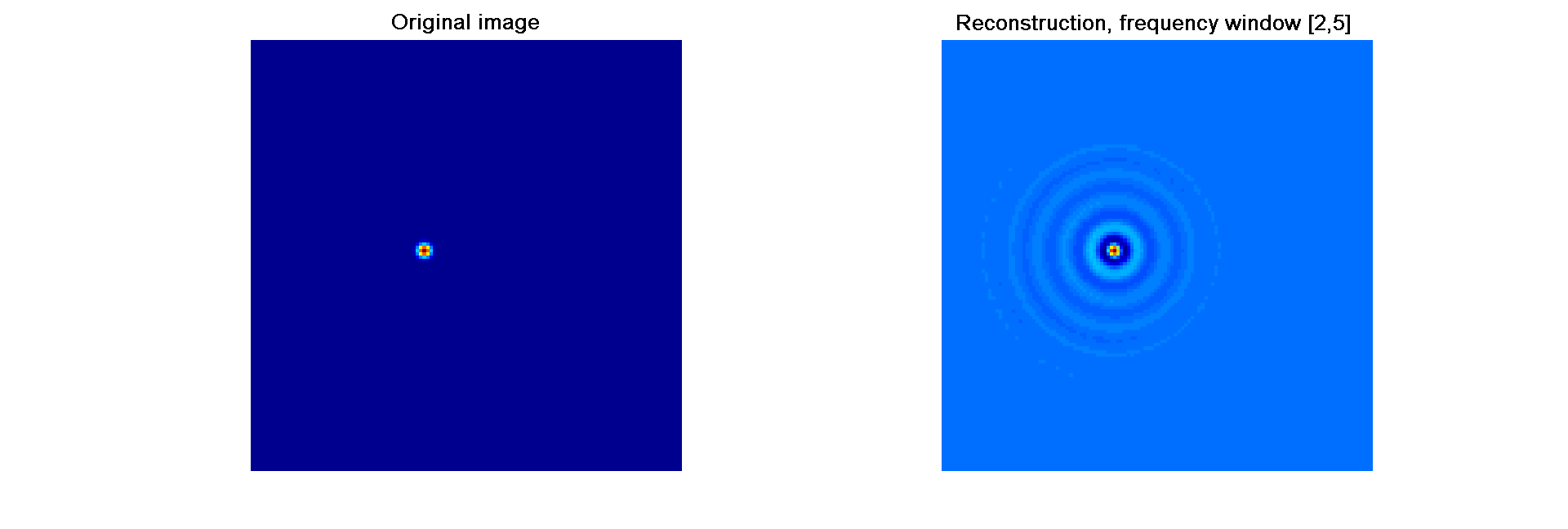
Figure 1: Point source (left) and textured reconstruction (right)

4 Photoacoustics with band-limited data

We create speckle patterns computationally from photoacoustic data using band-limited measurements for backprojection and approximating the initial source $f$. To be more precise, instead of measuring the exact trace of the solution of (6) at $\Gamma$, we instead assume to measure the bandlimited data $m=\phi*_{t}p$.

The mathematical background is an application of some results by Haltmeier [18, Lmm. 3.1] (see also [19, 20]) to convolution kernels which do not necessarily have compact support. Before we state the theorem, we define the Radon und Fourier transform:

Definition 1.

The Radon transform $\mathcal{R}\varphi(\theta,s)$ maps $\varphi({\bm{x}})$ to its integrals over hyperplanes in $\mathbb{R}^{n}$ with distance $s\in\mathbb{R}$ to the origin and unit normal vector $\theta\in S^{n-1}$. Namely,

$$\mathcal{R}\varphi(\theta,s)\,=\,\int_{\theta\cdot{\bm{y}}=s}\varphi({\bm{y}})d{\bm{y}}.$$ (12)

In the case $n=1$, the Radon transform corresponds to the absolute value of the function. In the case where $\varphi$ is rotationally symmetric, the Radon transform $\mathcal{R}\varphi$ is independent of $\theta$. We can therefore write

$$\mathcal{R}\varphi(\theta,s)=\phi(s)$$ (13)

for a suitable, even function $\phi:\mathbb{R}\to\mathbb{R}$.

Definition 2.

The $n$-dimensional Fourier transform $\widehat{\varphi}({\bm{\kappa}})$ of $\varphi$ is defined as

$$\widehat{\varphi}({\bm{\kappa}})\,=\,\int_{\mathbb{R}^{n}}\varphi({\bm{y}})e^{-\mathrm{i}{\bm{y}}\cdot{\bm{\kappa}}}d{\bm{y}}\;.$$ (14)

If not stated differently, the Fourier transform of a time-dependent function $q({\bm{x}},t)$ is with respect to the time variable, i.e.

$$\widehat{q}({\bm{x}},\kappa)\,=\,\int_{\mathbb{R}}q({\bm{x}},t)e^{-\mathrm{i}t\kappa}dt\;.$$

Now we are ready to state the theorem:

Theorem 1.

Let $p=\mathcal{P}f$ be a solution of (7) with initial pressure $f\in C^{\infty}_{c}(\mathbb{R}^{n})$. Furthermore, assume that $\,\Psi\in L^{p}(\mathbb{R}^{n})$, for some $p$ such that $1\leq p<n/(n-1)$, is a radially symmetric convolution kernel, i.e., $\Psi({\bm{x}})\,=\,\psi(|{\bm{x}}|)$. Then

$$(\mathcal{P}(\Psi*_{\bm{x}}f))({\bm{x}},t)\,=\,(\mathcal{R}\Psi*_{t}\mathcal{P}_{\mathrm{even}}f)({\bm{x}},t)\,,$$ (15)

for all ${\bm{x}}\in\mathbb{R}^{n}$, $t>0$. The convolution acts with respect to the ${\bm{x}}$-variable on the left hand side and with respect to the $t$-variable on the right hand side of (15), respectively.

Proof.

First we note that $\mathcal{P}(\Psi*_{\bm{x}}f)\in L^{p}(\mathbb{R}^{n})$: Since we have

$$\Psi*_{\bm{x}}\Delta f\,=\,\Delta(\Psi*_{\bm{x}}f),\quad\text{in }\mathbb{R}^{n}\times(0,\infty)\,,$$

we immediately conclude that

$$\mathcal{P}(\Psi*_{\bm{x}}f)=\Psi*_{\bm{x}}\mathcal{P}f,\quad\text{in }\mathbb{R}^{n}\times(0,\infty)\;.$$ (16)

Young’s inequality ensures that

$$L^{p}(\mathbb{R}^{n})*L^{1}(\mathbb{R}^{n})\,\subseteq\,L^{p}(\mathbb{R}^{n})\,,$$

so that

$${\mathcal{P}}(\Psi*_{\bm{x}}f)=\Psi*_{\bm{x}}\mathcal{P}f\in L^{p}(\mathbb{R}^{n})\,,$$

since $\mathcal{P}f\in C^{\infty}_{c}(\mathbb{R}^{n})\subseteq L^{1}(\mathbb{R}^{n})$ for every $t>0$. The rest of the proof is essentially the same as in [18, Lemma 3.1]: We start proving the result for one spatial dimension, i.e. $n=1$, and write here $x$ instead of ${\bm{x}}$ for the spatial variable. To avoid confusion later on, we write $\bar{\mathcal{P}}$ instead of $\mathcal{P}$ for the wave operator in one dimension. Using D’Alembert’s formula it follows that

$$\begin{aligned} &\bar{\mathcal{P}}\left(\Psi*_{x}f\right)(x,t)\\ &\,=\,\frac{1}{2}\left(\int_{\mathbb{R}}\psi(|y|)f(x-t-y)dy\,+\,\int_{\mathbb{R}}\psi(|y|)f(x+t-y)dy\right)\\ &\forall\,t>0\;.\end{aligned}$$

Then, by substituting $y$ by $-y$ in the first integral it follows that for all $t>0$,

$$\begin{aligned} &\bar{\mathcal{P}}\left(\Psi*_{x}f\right)(x,t)\\ &\,=\,\frac{1}{2}\left(\int_{\mathbb{R}}\psi(|y|)\big{(}f(x-(t-y))\,+\,f(x+(t-y))\big{)}dy\right)\;.\end{aligned}$$ (17)

According to D’Alembert’s formula,

$$\frac{1}{2}\big{(}f(x-(t-y))\,+\,f(x+(t-y))\big{)}=\bar{\mathcal{P}}f(x,t-y)\text{ for }t-y>0\;.$$

Due to our choice of extension to negative times in (10), we also have

$$\frac{1}{2}\big{(}f(x-(t-y))\,+\,f(x+(t-y))\big{)}=\bar{\mathcal{P}}_{\text{even}}f(x,t-y)\text{ for all }t\;.$$

Therefore, it follows from (17) that

$$\begin{aligned} \bar{\mathcal{P}}(\Psi*_{x}f)(x;t)\,&=\,\int_{\mathbb{R}}\psi(|y|)\bar{\mathcal{P}}_{\text{even}}f(x,t-y)dy\;.\end{aligned}$$ (18)

Using the definition of the Radon transform in 1D it follows then that

$$\bar{\mathcal{P}}(\Psi*_{x}f)(x;t)=\int_{\mathbb{R}}\mathcal{R}\psi(y)\bar{\mathcal{P}}_{\text{even}}f(x,t-y)dy\;.$$

For $n>1$ we note that for all $h\in C^{2}(\mathbb{R}^{n})$,

$$(\mathcal{R}\Delta h)(\theta,s)\,=\,(\partial_{s}^{2}\mathcal{R}h)(\theta,s)\,,\quad\text{ for all }s\geq 0\,,$$

see e.g. [21, p.3]. By applying the Radon transform to the wave equation, we can therefore conclude

$$\left(\mathcal{R}\mathcal{P}f\right)(\theta,s;t)\,=\,\left(\bar{\mathcal{P}}\mathcal{R}f\right)(\theta,s;t)\;.$$ (19)

Now we use the convolution theorem of the Radon transform (see e.g. [31]), which states that

$$\mathcal{R}(f*_{\bm{x}}g)(\theta,s)=(\mathcal{R}f*_{s}\mathcal{R}g)(\theta,s),$$ (20)

where the convolution on the left-hand is $n$-dimensional, whereas the convolution on the right-hand side is taken in one dimension. By applying (16), (20) and (19), (16) and (18), and again (19), it follows that:

$$(\mathcal{R}\mathcal{P})(\Psi*_{\bm{x}}f)\, =\,\mathcal{R}\Psi*_{s}\bar{\mathcal{P}}\mathcal{R}f\,=\,(\mathcal{R}\Psi)*_{t}(\bar{\mathcal{P}}_{\text{even}}\mathcal{R}f)$$

$$=\,(\mathcal{R}\Psi)*_{t}(\mathcal{R}\mathcal{P_{\text{even}}}f).$$

The term $\mathcal{R}\Psi=\phi(|\cdot|)$ on the right-hand-side is independent of $\theta$ due to the rotational symmetry of $\Psi$. We therefore can write (see also Remark 1):

$$(\mathcal{R}\mathcal{P})(\Psi*_{\bm{x}}f)(\theta,s;t)\, =\,\mathcal{R}\big{(}\phi(|\cdot|)*_{t}\mathcal{P}f\big{)}(\theta,s;t).$$ (21)

Due to our choice of $p$, the Radon transform is injective on $L^{p}(\mathbb{R}^{n})$ (see [47]). From (21), we therefore derive (15). ∎∎

Theorem 1 is the main ingredient to relate the convolved measurement data with a convolution of $f$. Note, however, that on the right-hand side of statement (15), the quantity $\mathcal{P}_{\text{even}}f$ appears, whereas our measurements give only knowledge of $\phi*\mathcal{P}f$ as in (11). For application of Theorem 1 to our case of bandlimited data, we therefore need a relation between $\mathcal{P}_{\text{even}}f$ and $\phi*\mathcal{P}f$, which is provided by the following corollary.

Corollary 1.

Let $\Psi:\mathbb{R}^{n}\to\mathbb{R}$ be radially symmetric and $\Psi\in L^{p}(\mathbb{R}^{n})$, for some $1\leq p<n/(n-1)$, and let $\mathcal{R}\Psi$ be represented as

$$\mathcal{R}\Psi(\theta,s)\,=\,\Phi(\theta,|s|)\,=\,\phi(|s|)\,,$$

for an even function $\phi:\mathbb{R}\to\mathbb{R}$ as in (13). Moreover, let our measurements be given by

$$m({\bm{x}};t)=(\phi*_{t}\mathcal{P}f)({\bm{x}};t)\quad\text{on }\Gamma\times(0,\infty)\;.$$

Then, the function

$$m_{\text{even}}({\bm{x}},t):=(\phi*_{t}P_{\text{even}}f)({\bm{x}},t)\quad\text{on }\Gamma\times(0,\infty)\,,$$ (22)

where ${\bm{x}}\in\Gamma$, $t\in(0,\infty)$, can be computed analytically from the causal measurement data $m({\bm{x}},t)$. Furthermore,

$$m_{\text{even}}({\bm{x}};t)\,=\,(\mathcal{P}(\Psi*_{\bm{x}}f))({\bm{x}},t)\quad\text{on }\Gamma\times(0,\infty)\;.$$ (23)

Proof.

Let $p$ denote the solution of (6). Since $p({\bm{x}};t)$ is real-valued, it follows that

$$\widehat{p}({\bm{x}},-\kappa)\,=\,\overline{\widehat{p}({\bm{x}},\kappa)}\,\qquad\forall x\in\mathbb{R}^{n},\kappa\in\mathbb{R}\,,$$

and therefore

$$\widehat{\mathcal{P}_{\text{even}}f}({\bm{x}},\kappa)\,=\,2\,{\rm Re\,}(\hat{p}({\bm{x}},\kappa))\,\qquad\forall{\bm{x}}\in\mathbb{R}^{n},\kappa\in\mathbb{R}\,.$$

Thus, from (22) it follows that

$$\widehat{m_{\text{even}}}({\bm{x}},\kappa) =\,\widehat{\phi}(\kappa)\widehat{\mathcal{P}_{\text{even}}f}({\bm{x}},\kappa)$$

$$=\,\widehat{\phi}(\kappa)\,2\,{\rm Re\,}\left(\widehat{\mathcal{P}f}({\bm{x}},\kappa)\right)$$

$$=\,2\,{\rm Re\,}\left(\widehat{\phi}(\kappa)\,\widehat{\mathcal{P}f}({\bm{x}},\kappa)\right)$$

$$=\,2\,{\rm Re\,}\left(\widehat{m}({\bm{x}},\kappa)\right)\qquad\forall{\bm{x}}\in\Gamma,\,\forall\kappa\in\mathbb{R}\,,$$

where in the third equality we use that $\widehat{\phi}$ is real-valued, since $\phi$ is a real-valued and even function. The function $m_{\text{even}}=\phi*_{t}\mathcal{P}_{\text{even}}f$ is of the appropriate form to apply (15), which allows us to derive (23). ∎∎

Corollary 1 gives a simple relation between causal and even data convolved in time. Using Theorem 1, the even data can be related to an initial source convolved in space by a point-spread function (PSF) that is given in terms of an inverse Radon transform of the radially symmetric extension of the impulse-response function (IRF), previously denoted by the letter $\phi$.

5 PAI elastography using texture information

The results of Section 4 give the theoretical description for the influence of using band-limited data in the photoacoustic reconstruction. In the following subsection, we describe how to find pairs of filter functions $\phi$ and $\Psi$ in practice. Moreover, we give an example of a pair of oscillating functions, that we use in what follows to create speckle-like patterns on photoacoustic images. The rest of the paper will treat the case of two spatial dimensions. Since the theoretical considerations from Section 4 are valid in any spatial dimension, the application to 3D images works in complete analogy to the two-dimensional case described below.

5.1 Speckle generation in 2D Photoacoustics

We assume to measure the bandpass data

$$m=\phi*_{t}\mathcal{P}f\,,$$

where we choose $\phi$ as follows: The time-domain equivalent of the bandpass

$$\widehat{\phi}({\bm{x}},\kappa)=\chi_{[\kappa_{\text{min}},\kappa_{\text{max}}]}(|\kappa|)$$ (24)

is given by the IRF

$$\begin{aligned} \phi(t)=\,\frac{\cos(\kappa_{0}t)}{2a}\mathrm{sinc}\left(\frac{t}{4\pi a}\right),\end{aligned}$$ (25)

where $2a=\kappa_{\text{max}}-\kappa_{\text{min}}$ is the bandwidth and $\kappa_{0}=\kappa_{\text{min}}+a$ is the center frequency of our window. Note that with the formulation above, we cover the cases where our detector measures the described signal as well as the case where we manipulate the data by a post-processing step.

Now assume that we have computed $m_{\text{even}}$ as described in Corollary 1. The results of Section 4 in principle describe the relationship of the filter in time and a resulting filter in space. But since we actually want to compute this space filter explicitly, it is convenient to make use of the so-called Fourier-slice theorem for the Radon transform [21, 47], that relates the Fourier transform of the Radon transform (in radial direction) to the Fourier transform of the image (in all spatial dimensions). In 2D, the Radon transform of a radially symmetric function is nothing else than the Abel transform [31]. The Fourier-transform of a two dimensional radially symmetric function is the so-called Hankel transform. The 2D version of the Fourier slice theorem for radially symmetric functions is therefore often written as

$$\mathcal{F}\mathcal{A}=\mathcal{H},$$

also called the FHA-cycle. In order to find the corresponding $\Psi$ to the function $\phi$ in (24), we make use of the tables in literature describing important pairs of the above mentioned Fourier, Abel and Hankel transforms (see, e.g., [7, 36]). In fact, for our given hard bandpass (24), it suffices to compute its (inverse) Hankel transform, so that the corresponding point-spread function $\Psi$ is given by

$$\begin{aligned} \Psi({\bm{x}})=\,\frac{2\pi}{|{\bm{x}}|}\left[(\kappa_{\text{max}})J_{1}\left((\kappa_{\text{max}})|{\bm{x}}|\right)-(\kappa_{\text{min}})J_{1}\left((\kappa_{\text{min}})|{\bm{x}}|\right)\right]\;,\end{aligned}$$ (26)

where $J_{1}$ is the first-kind Bessel function of order $1$. By using an asymptotic estimate of $J_{1}$ for large arguments, it is easy to check that $\Psi\in L^{p}(\mathbb{R}^{2})$ iff $p>4/3$, which means that $\Psi$ fulfils the integrability requirements demanded in Corollary 1. This ensures that the result actually applies to the used filter.

Our suggested approach for texture generation then is this: We choose $\kappa_{\text{max}}$ and $\kappa_{\text{min}}$ to determine the IRF $\phi$. Then we compute $m_{\text{even}}$ and solve the photoacoustic inverse problem with data $m_{\text{even}}$. Theorem 1 then ensures that this yields the perturbed reconstruction

$$f*_{\bm{x}}\Psi$$ (27)

With the right choice of $\kappa_{\text{min}}$ and $\kappa_{\text{max}}$, this is a natural candidate for a textured variant of the photoacoustic contrast in the initial pressure $f$.

In Figure 1, a point source and its photoacoustic reconstruction from band-limited data (i.e., data convolved with the IRF in (25)) are shown. The oscillations introduced by the present band-limited photoacoustic reconstruction method introduce additional texture on the image. The use of this texture in estimating the optical flow between two photoacoustic images is investigated in the following sections.

5.2 Principle of PAI elastography

In the previous subsection, we introduced a texture method for photoacoustic images. We now will study how motion estimation can be performed and amended by adding texture to photoacoustic images.

We emphasize that the initial pressure $f$ introduced in (6) in the photoacoustic forward problem is spatially varying and can either represent the image before (i.e., $f_{1}$) or after ($f_{2}$) mechanical deformation as described in Section 2.2.

The main concept in the proposed method of photoacoustic elastography is to perform the following steps in the first step in section 2.1:

• record a PAI image $f_{1}$ using the texture-generating method

• perturb the tissue using a mechanical source

• record the perturbed configuration $f_{2}$ using the texture-generation method

We will now estimate the displacement $\mathbf{u}$ as in the second step in section 2.1.

In the following, we evaluate the motion estimation using the Horn-Schunck model (4) with or without speckle generation.

6 Experiments

There are many different varieties of experiments one can perform. In this section, we present a first selection, using structures which contain homogeneous regions, similar to vascular structures.

6.1 Simulations

We simulate photoacoustic forward data using the k-wave toolbox [49]. For reconstruction, we use a filtered back-projection algorithm. Displacement vector fields have been simulated using the FEM and mesh-generating packages GetDP and Gmsh [9, 17].

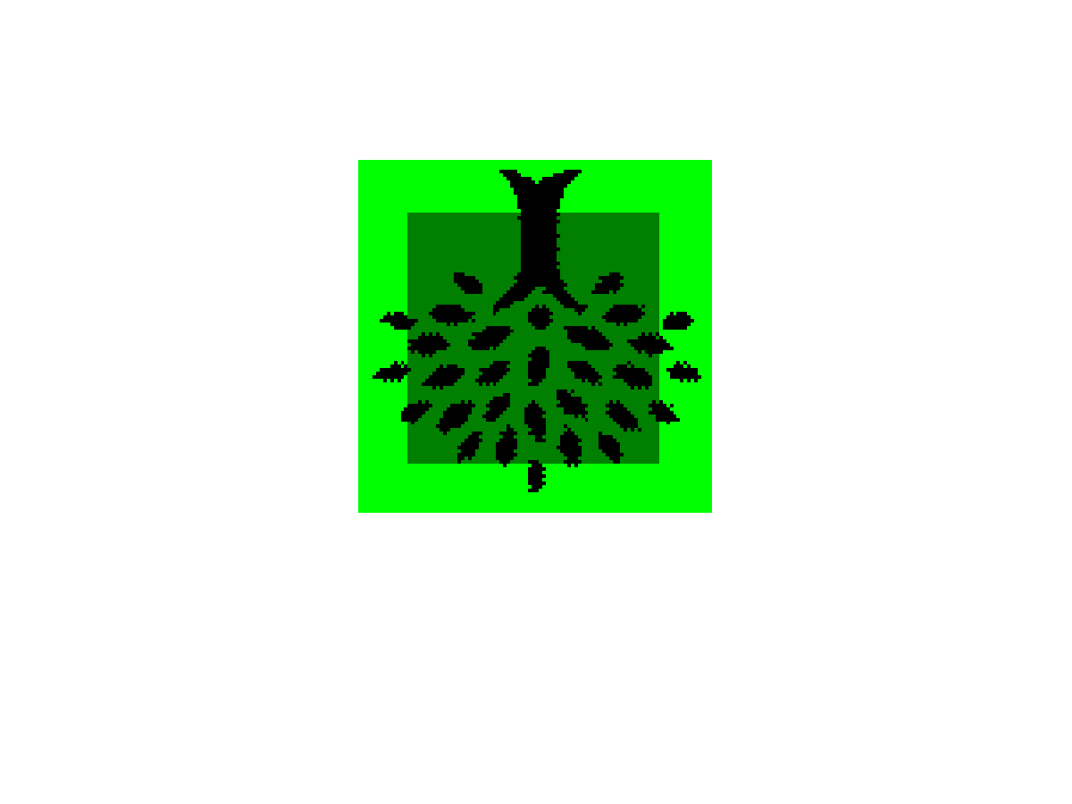
(a) Visualized mask

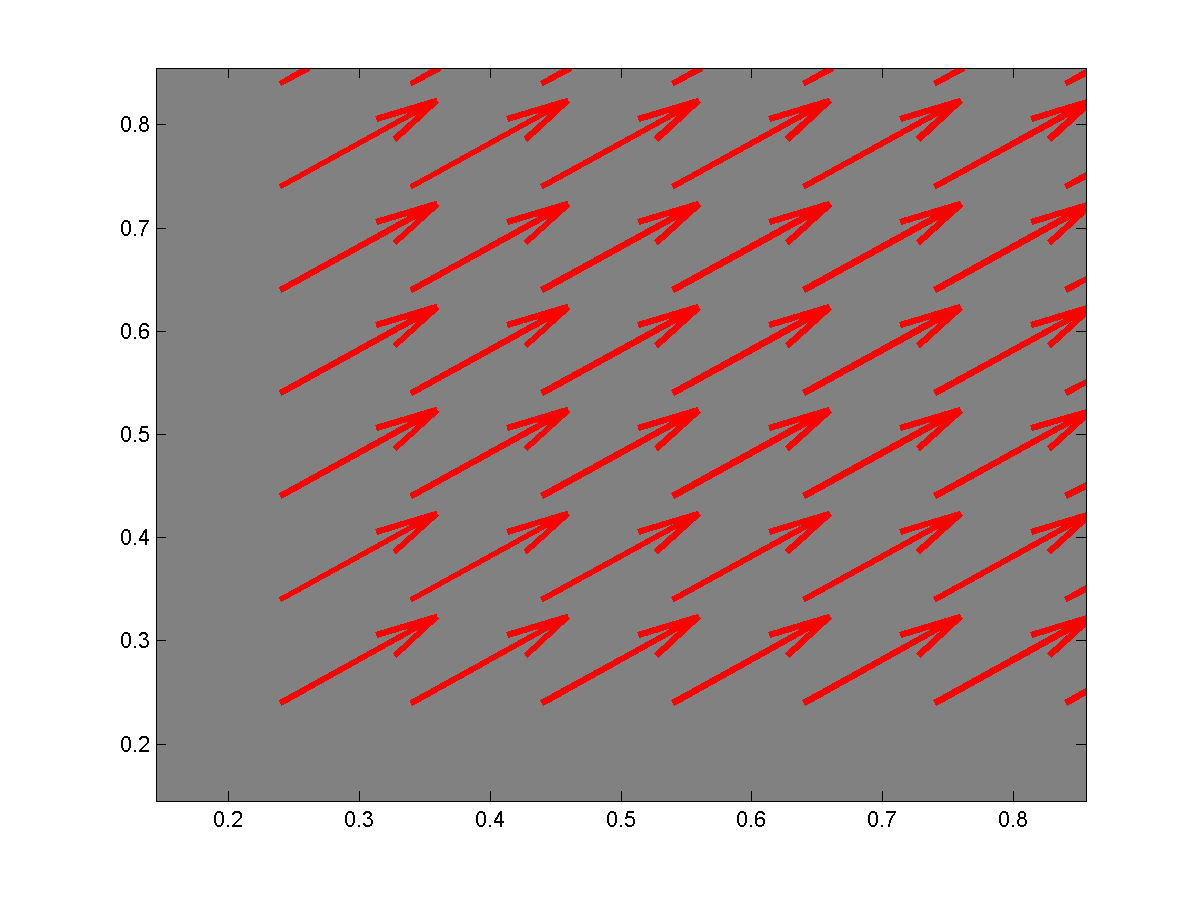
(b) Ground truth

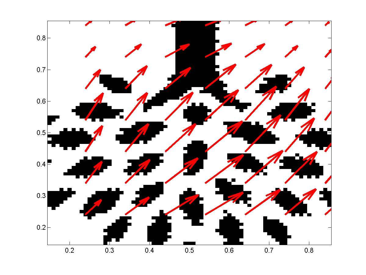
(c) none

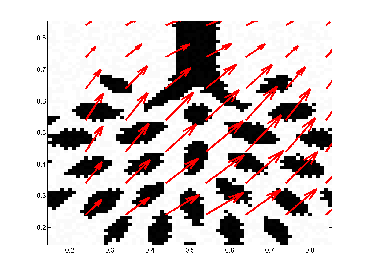
(d) Gauss $\alpha=0.3$

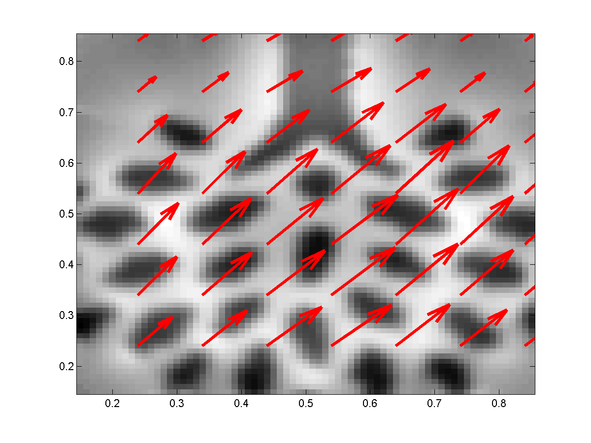
(e) Band $\kappa_{\text{min}}=0.4$

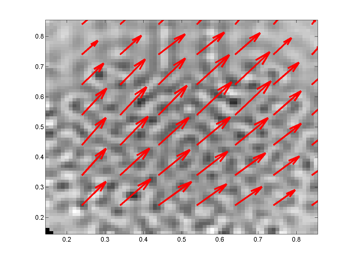
(f) Band $\kappa_{\text{min}}=1.8$

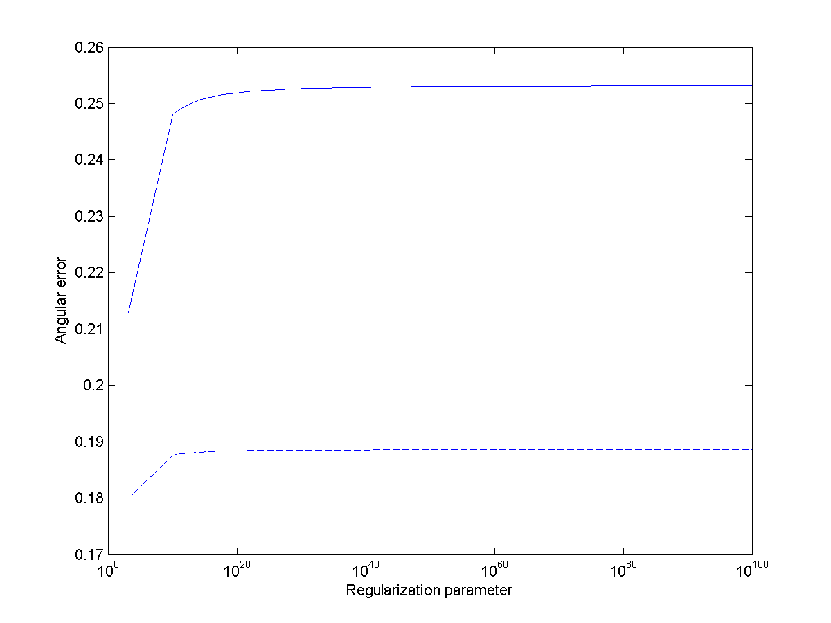
(g) Angular error

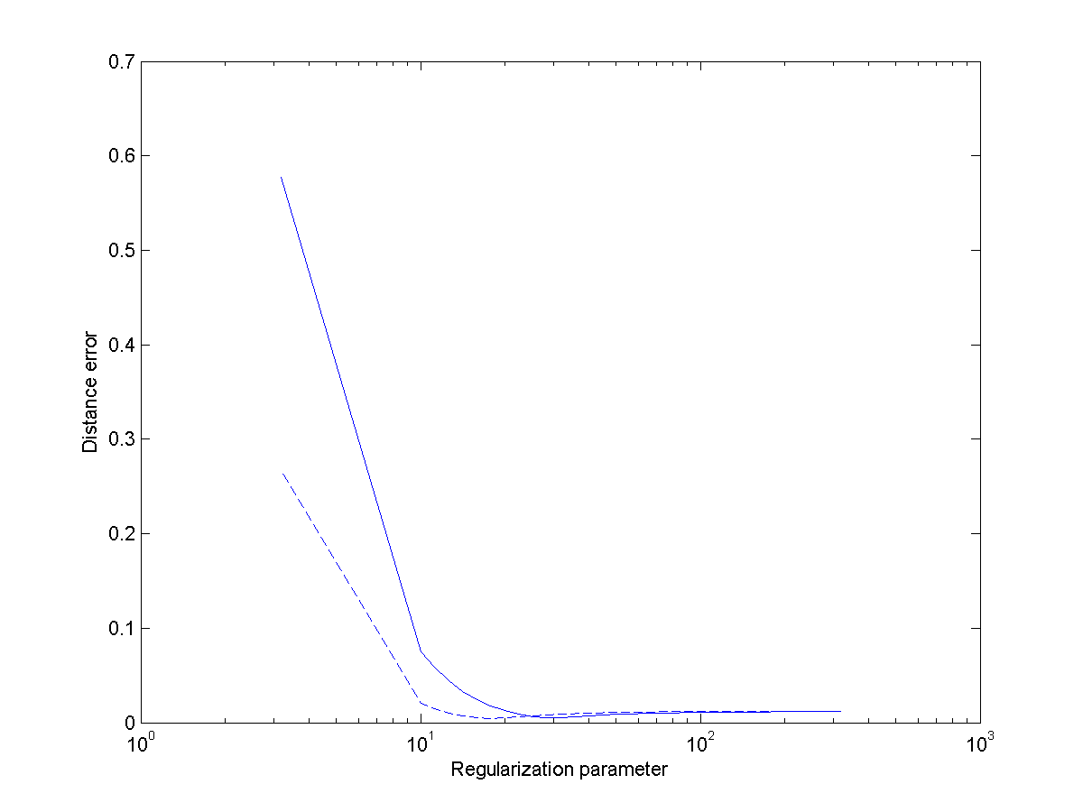
(h) Distance error

Figure 2: (Experiment 1) (c)-(f): Computed vector fields for $\lambda=12.5893$. (g), (h): different error measures for regularization parameters $10^{0.5}\leq\lambda\leq 10^{2.5}$, full line: original data; dashed line: band-limitation texture $\kappa=0.4$

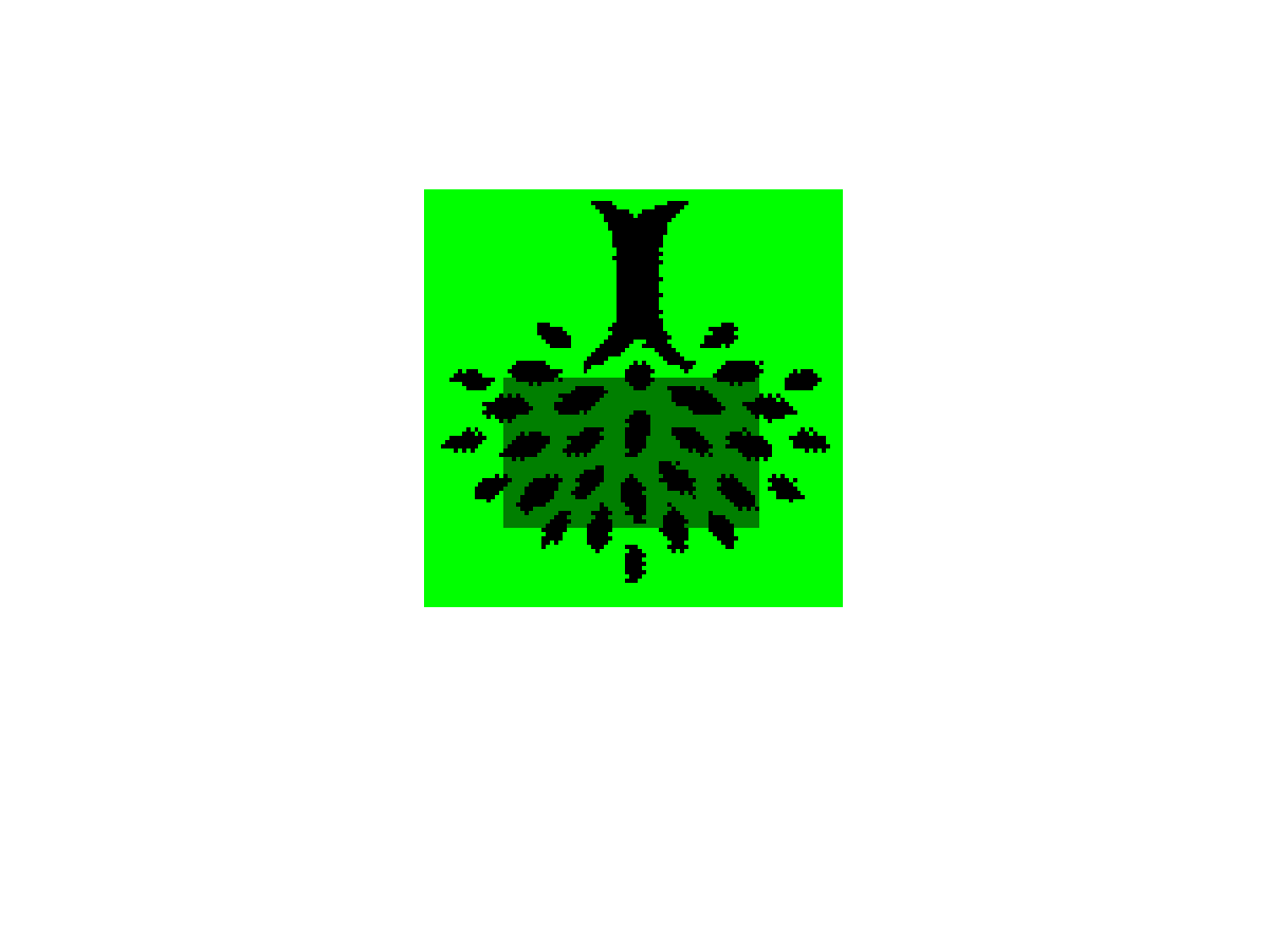
(a) Visualized mask

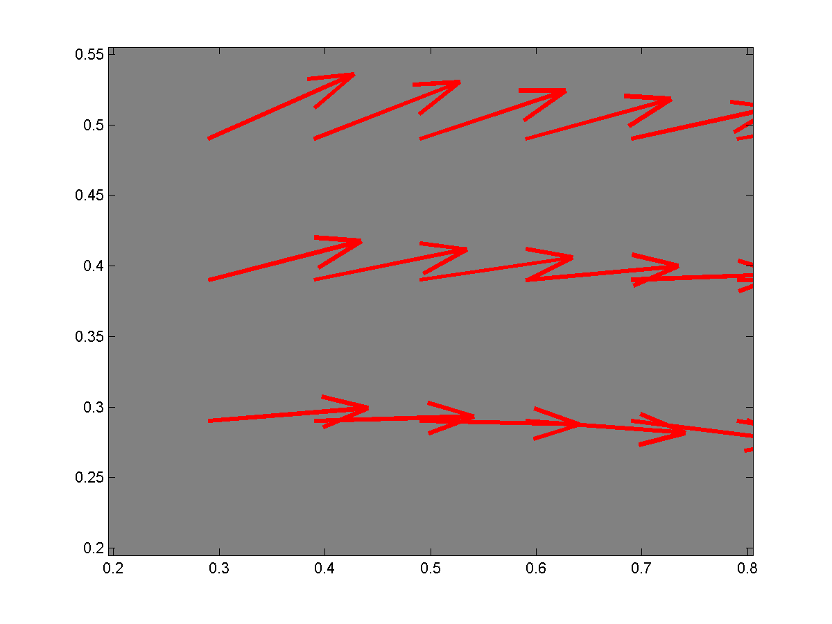
(b) Ground truth

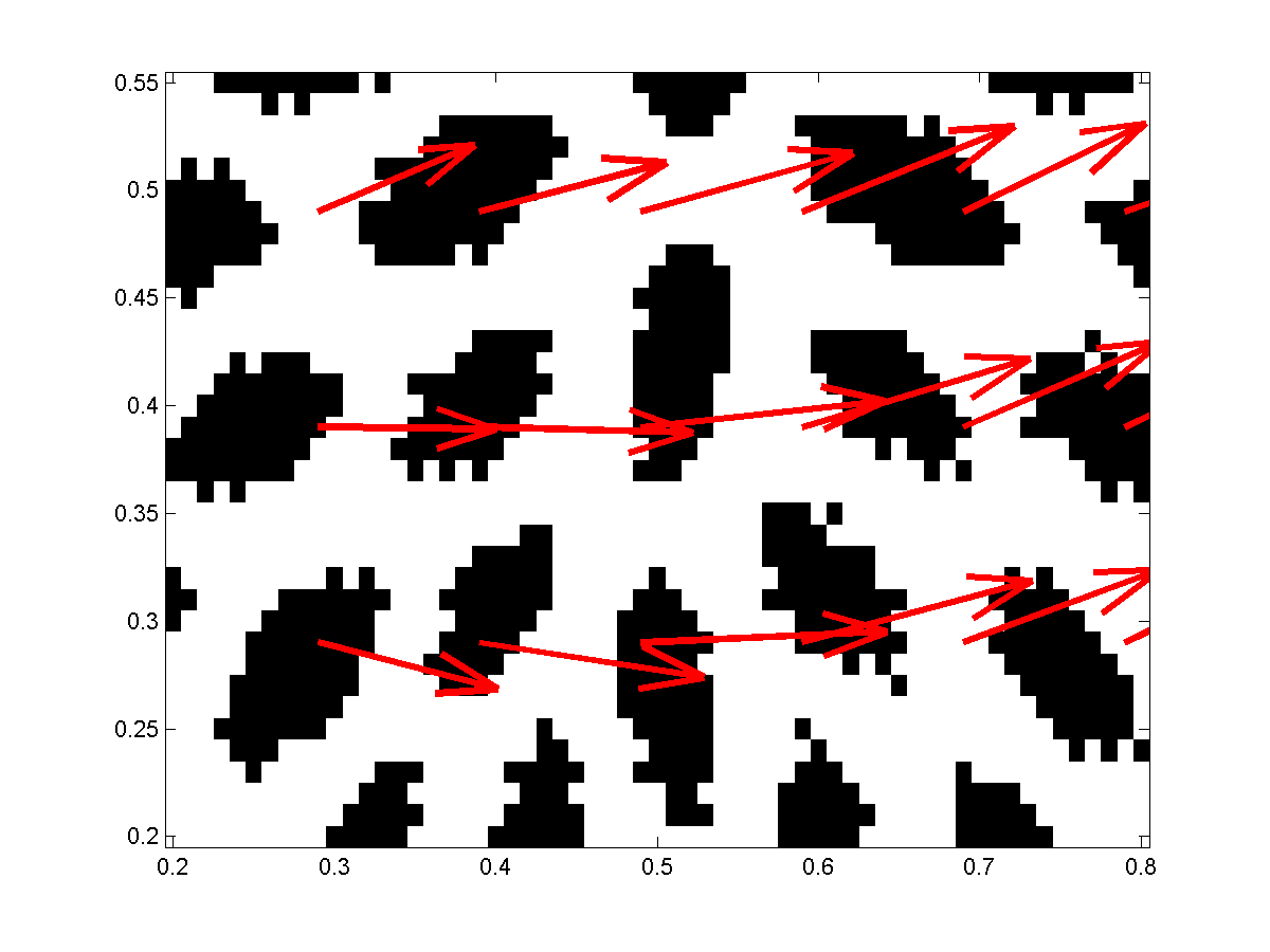
(c) none

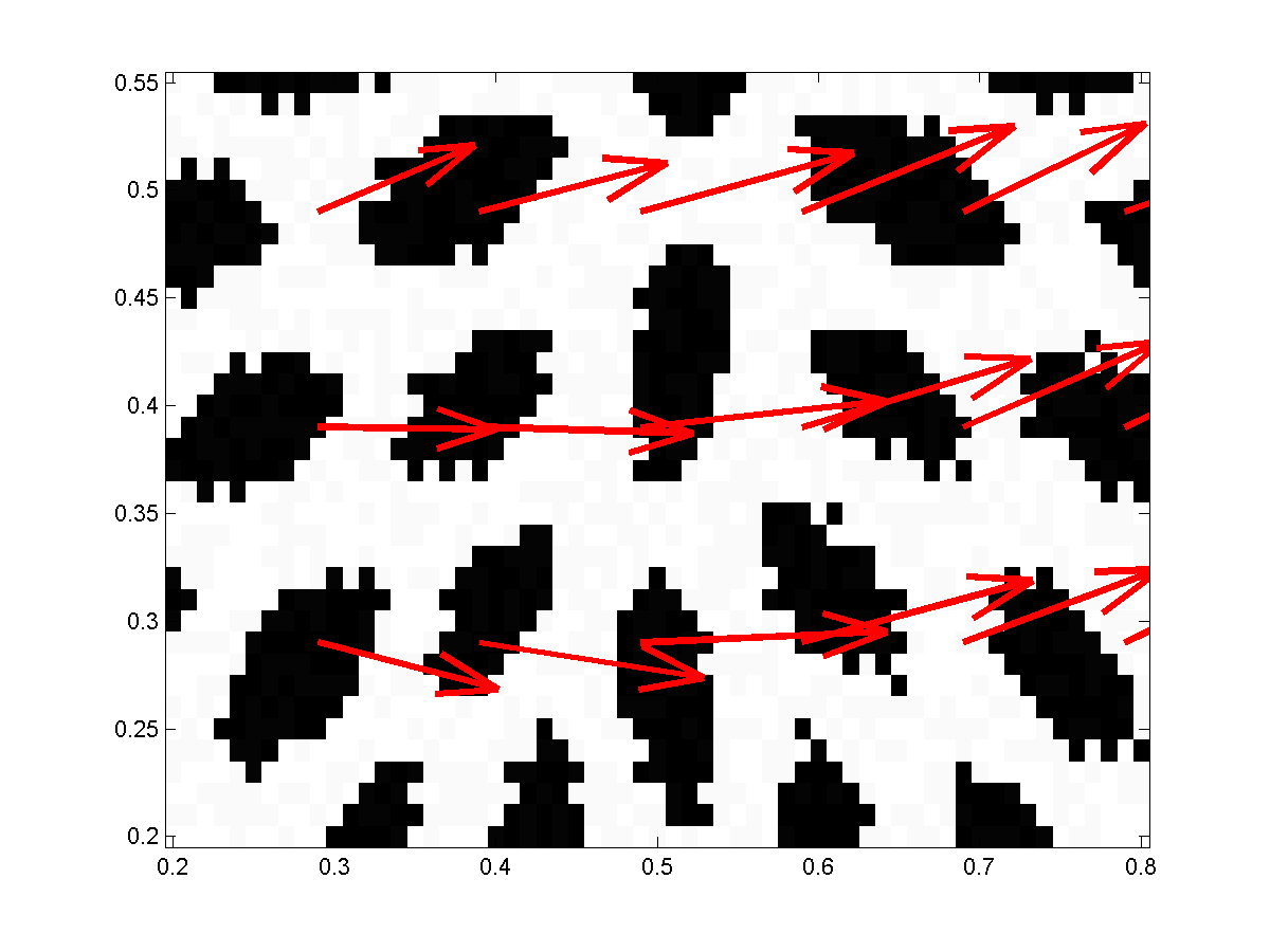
(d) Gauss 0.3

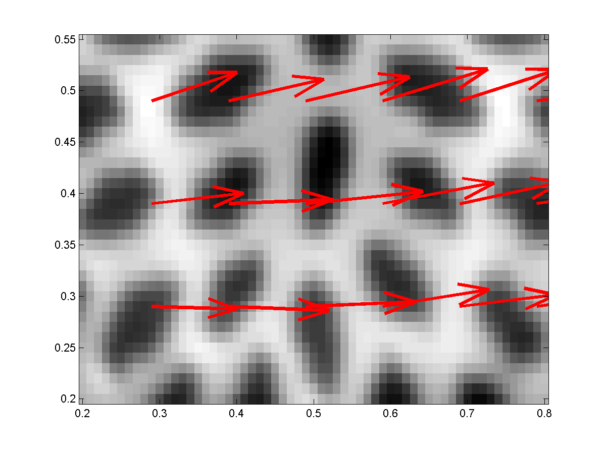
(e) Band 0.4

(f) Band 1.8

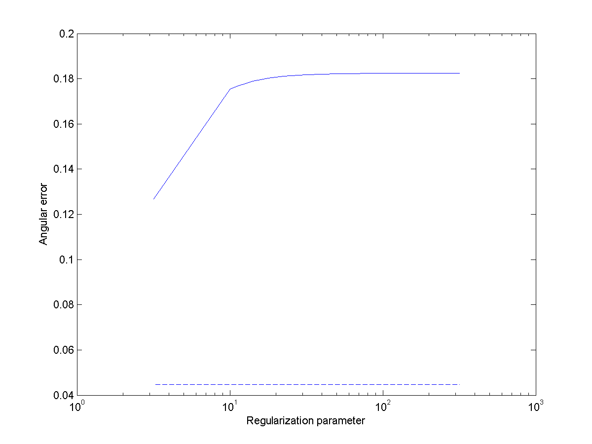
(g) Angular error

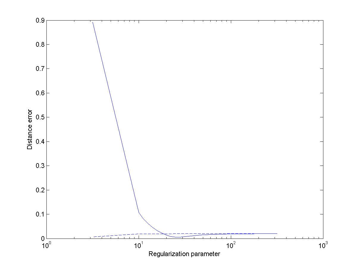
(h) Distance error

Figure 3: (Experiment 2) (c)-(f): Computed vector fields for $\lambda=12.5893$. (g), (h): different error measures for regularization parameters $10^{0.5}\leq\lambda\leq 10^{2.5}$, full line: original data; dashed line: band-limitation texture $\kappa=1.8$

Table 1: Experiments 1 and 2: Error analysis

Texture Mode	AAE	AEEabs	AEErel	Warping
none	0.2499	0.0445	3.3232	0.3739
Gauss 0.3	0.2499	0.0445	3.3237	0.3797
Band 0.4	0.1880	0.0101	0.7548	0.0737
Band 1.8	0.2382	0.0114	0.8546	0.0345

(a) Rigid experiment, $\lambda=12.5893$ (see Figure 2)

Texture Mode	AAE	AEEabs	AEErel	Warping
none	0.1780	0.0617	2.9980	0.4886
Gauss 0.3	0.1784	0.0617	2.9990	0.4923
Band 0.4	0.0928	0.0135	0.6595	0.1189
Band 1.8	0.0447	0.0190	0.9232	0.0494

(b) Non-rigid experiment, $\lambda=12.5893$ (see Figure 3)

6.2 Material, displacement and parameters

The synthetic material was chosen to exhibit homogeneous regions surrounded by edges. In each experiment, we evaluated a rigid deformation and a non-rigid deformation.

In Experiments 1 and 2, we use a tree structure designed by Brian Hurshman and licensed under CC BY 3.0.

6.3 Texture Modes

The purpose of experiments is to evaluate the influence of the texture pattern introduced by (27) to the images, using the basic filtered-backprojection reconstruction of the image.

Letting $\kappa_{\text{max}}=10$, we choose different values of choose $\kappa_{\text{min}}$ and record the error with respect to the measures defined below 6.4.

On the one hand, these are compared with the motion reconstructions from the unperturbed images. On the other hand, we compare the pictures to the following Gaussian texture explained in the sequel.

We will produce the Gaussian texture in the image as follows: We take an image $f(\mathbf{x})$ and apply Gaussian noise to the image $f$, producing a reference image

$$f_{1}(\mathbf{x})=f(\mathbf{x})+\alpha\;r(\mathbf{x}),$$ (28)

where $\alpha$ is a constant and $r(\mathbf{x})$ is a noise function governed by Gaussian noise. Then we warp the textured image using a certain vector field $\mathbf{u}$, producing the reference image $f_{1}$ and the target image

$$f_{2}(\mathbf{x})=f_{1}(\mathbf{x}+\mathbf{u}(\mathbf{x})).$$ (29)

At last, we compute the optical flow between $f_{1}$ and $f_{2}$ and then determine whether the computed field is approximately the correct motion field.

We emphasize that due to (28) and (29), the artificial texture pattern thus introduced behaves like a material characteristic which is advected by the vector field $\mathbf{u}$.

In contrast to that, the in using the texture method (27), we have recourse to the principle outlined in section 5: to arrive at the target image $f_{2}$

• (sec. 5, step b) the mechanical deformation is applied

• (sec. 5, step c) the texture method is applied.

6.4 Validation

The field which is computed with the optical flow algorithm should approximately match the correct motion field. In order to study how PAI and textured PAI images behave under mechanical deformations, we adopt the following validation procedure:

Synthectic Data verification

• Choose a particular vector field $\mathbf{u}_{0}$, as well as a reference image $f_{1}$

• Compute the warped image $f_{2}$ by interpolation, i.e. $f_{2}=f_{1}(\mathbf{x}+\mathbf{u}_{0}(\mathbf{x}))$

• Compute the optical flow $\mathbf{u}(\mathbf{x})$ from $f_{1}$ and $f_{2}$

• Compare the result $\mathbf{u}$ against the ground-truth vector field $\mathbf{u}_{0}$

Error measures

To compare the computed flows produced to the ground truth field, we use the angular and distance error, and to assess the prediction quality of the flow, we calculate the warping error. To define these error measures, write

$$\mathbf{u}_{0}(\mathbf{x}) =r_{0}(\mathbf{x})\;e^{i\varphi_{0}(\mathbf{x})}$$

$$\mathbf{u}(\mathbf{x}) =r(\mathbf{x})\;e^{i\varphi(\mathbf{x})}.$$

Then we define the

• average angular error (AAE)

  $$\int_{\Omega}|\varphi(\mathbf{x})-\varphi_{0}(\mathbf{x})|d\mathbf{x}$$

• average endpoint error (AEE)

  $$\int_{\Omega}\|\mathbf{u}-\mathbf{u}_{0}\|d\mathbf{x}$$

• average relative endpoint error (AEErel)

  $$\int_{\Omega}\frac{1}{\|\mathbf{u}_{0}\|}\|\mathbf{u}-\mathbf{u}_{0}\|d\mathbf{x}$$

• warping error

  $$\int_{\Omega}\|f_{2}(\mathbf{x})-f_{1}(\mathbf{x}+\mathbf{u}(\mathbf{x}))\|d\mathbf{x}.$$

7 Discussion

As mentioned in the introduction, elastography often relies on speckle tracking methods, including correlation techniques and optical flow. It is clear that such methods have a problem with homogeneous regions. As for the optical flow, this can be seen from (2), where the data term for homogeneous regions gives no information.

In Experiments 1-4, we used several pieces of synthetic data showing homogeneous regions and investigated the effect of the homogeneity in several regions of the data (see Figs. 2a-5a.

The visualization of the computed motion fields in Figs. 2c, 3c, 4c and 5c shows aberrations from the respective ground truth fields. Comparing the values for the angular, distance and warping errors in Table 1 to 2 shows these aberrations, if one restricts to the untextured original images.

We then applied the texture generation methods introduced in Section 5. The results in section 6 show that addition of texture is able to alleviate this problem of homogeneous regions to a considerable amount. The effect shows up in the different error types.

For the specimens we used, the angular error decreases about 20-30 % compared to the original error, and in extreme cases the decrease is as high as 75 % (as seen from Table 1b). As seen from Figs. 2h-5h, where the errors were plotted as a function of the regularization parameters, the distance error and in the warping error reach their minimum in the textured variant at lower regularization values than the original data. In this context, we note that the angular error is a monotonically increasing function of the regularization parameters in the cases we investigated. In some cases (as seen from Fig. 2h and Fig. 4h), the textured versions give also a lower distance error for the optimal regularization value; in other cases, with the motion estimation we used, the distance error is about the same magnitude as in the original versions.

The optimum frequency windows for the texture generating method also seem to differ for the rigid and the non-rigid deformations we used. Whereas for the rigid deformations, the window with $\kappa_{\text{min}}=0.4$ gave better results, the non-rigid deformations gave better results with $\kappa_{\text{min}}=1.8$.

The effect of adding texture seems to come from a filling-in-effect in the optical flow equation (2). Although the regularization term is responsible for such an interpolation usually, here this filling-in-effect originates from the data term; the function $\Psi$ seems to propgate the information from within the objects out across the edges and boundaries. This seems also to alleviate the aperture problem in optical flow, as the new texture creates also new gradients around edges. This may account for the lessening of the angular error.

Overall, the results point at the phenomenon that an effect which has deteriorating the image quality in one contrast (here the photoacoustic contrast) can have an advantageous effect on another contrast (here the mechanical contrast, which is inherent in the displacement $\mathbf{u}$).

8 Conclusion

We studied the topic of texture generation in photoacoustics, and applied bandwidth filter techniques for generating such texture in the reconstructed images. This kind of texture was mathematically characterized. Then we tested an application of the PAI texture for elastography purposes. It turned out that the texture generation technique has the potential to fill in otherwise untextured regions. The displacements can be better measured then, making photoacoustic elastography viable.

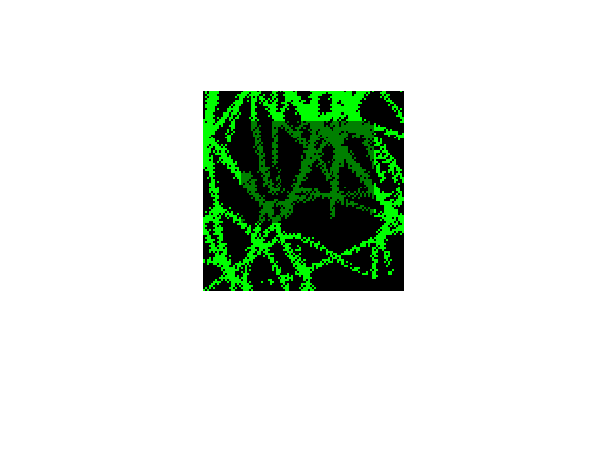
(a) Visualized mask

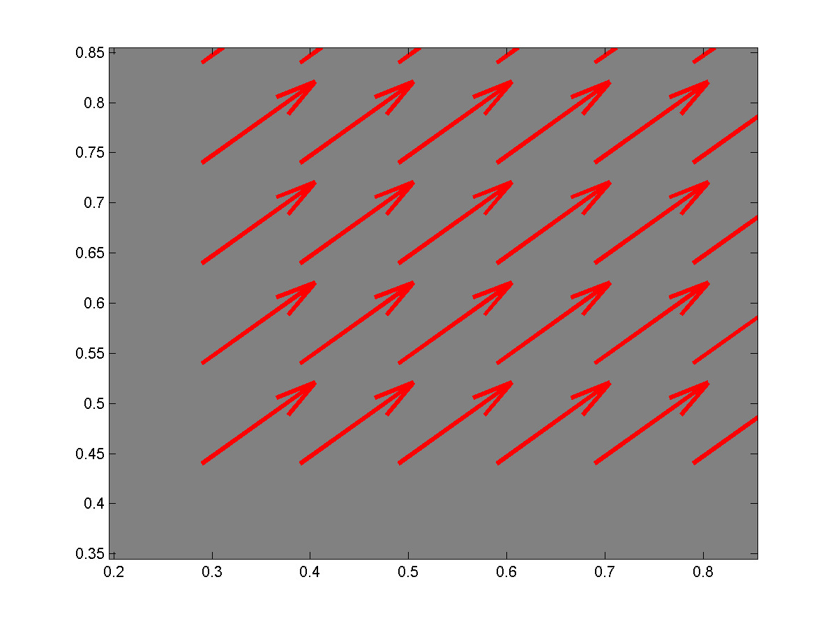
(b) Ground truth

(c) none

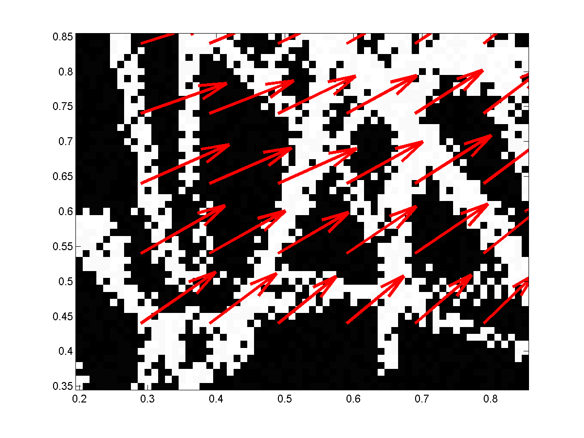
(d) Gauss $\alpha=0.3$

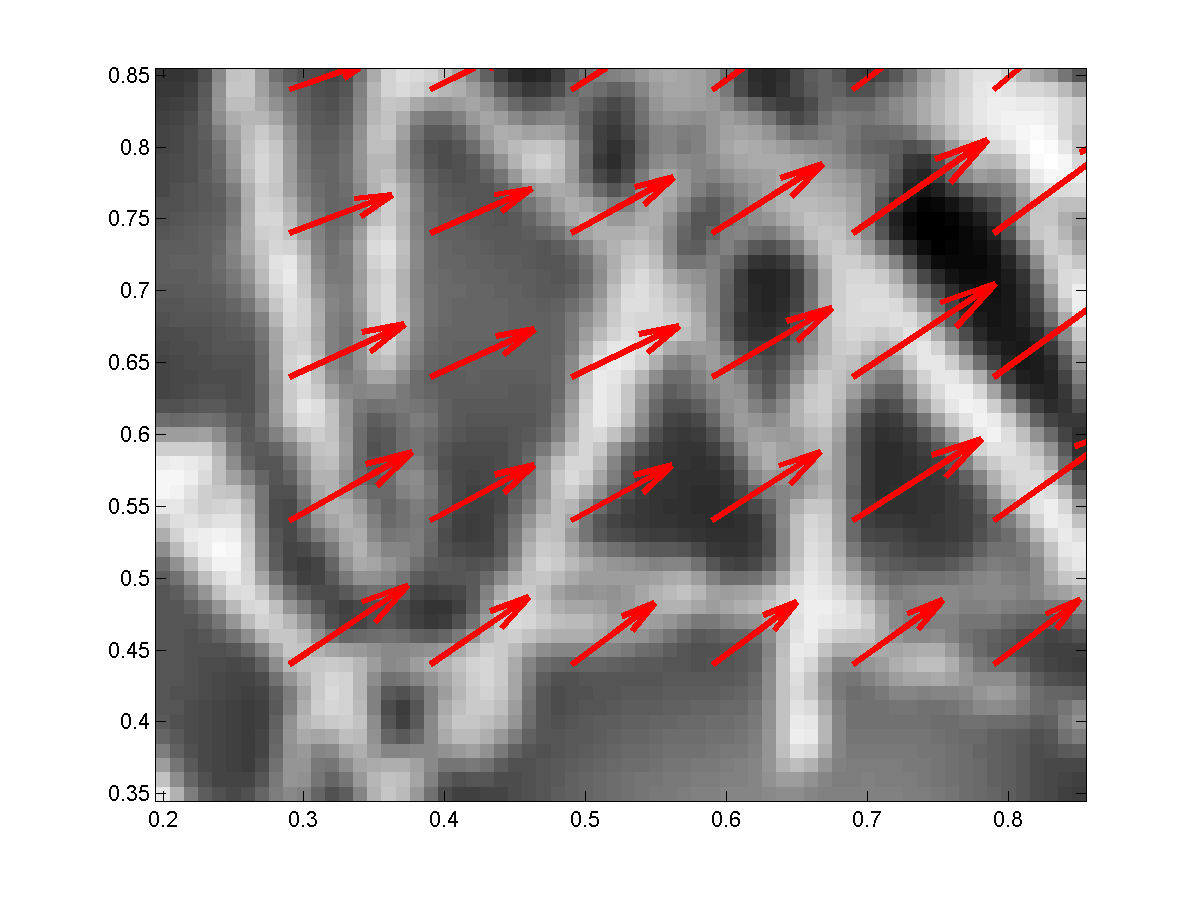
(e) Band $\kappa_{\text{min}}=0.4$

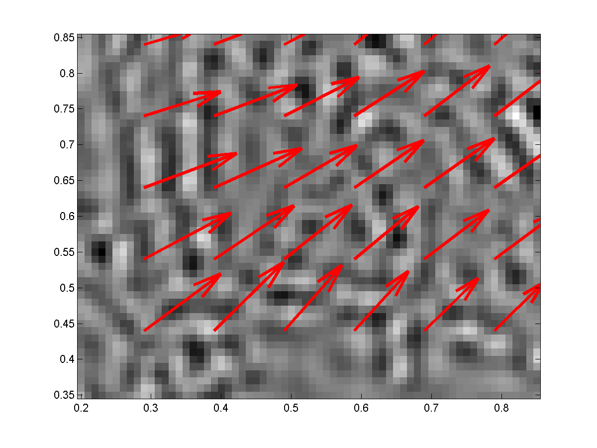
(f) Band $\kappa_{\text{min}}=1.8$

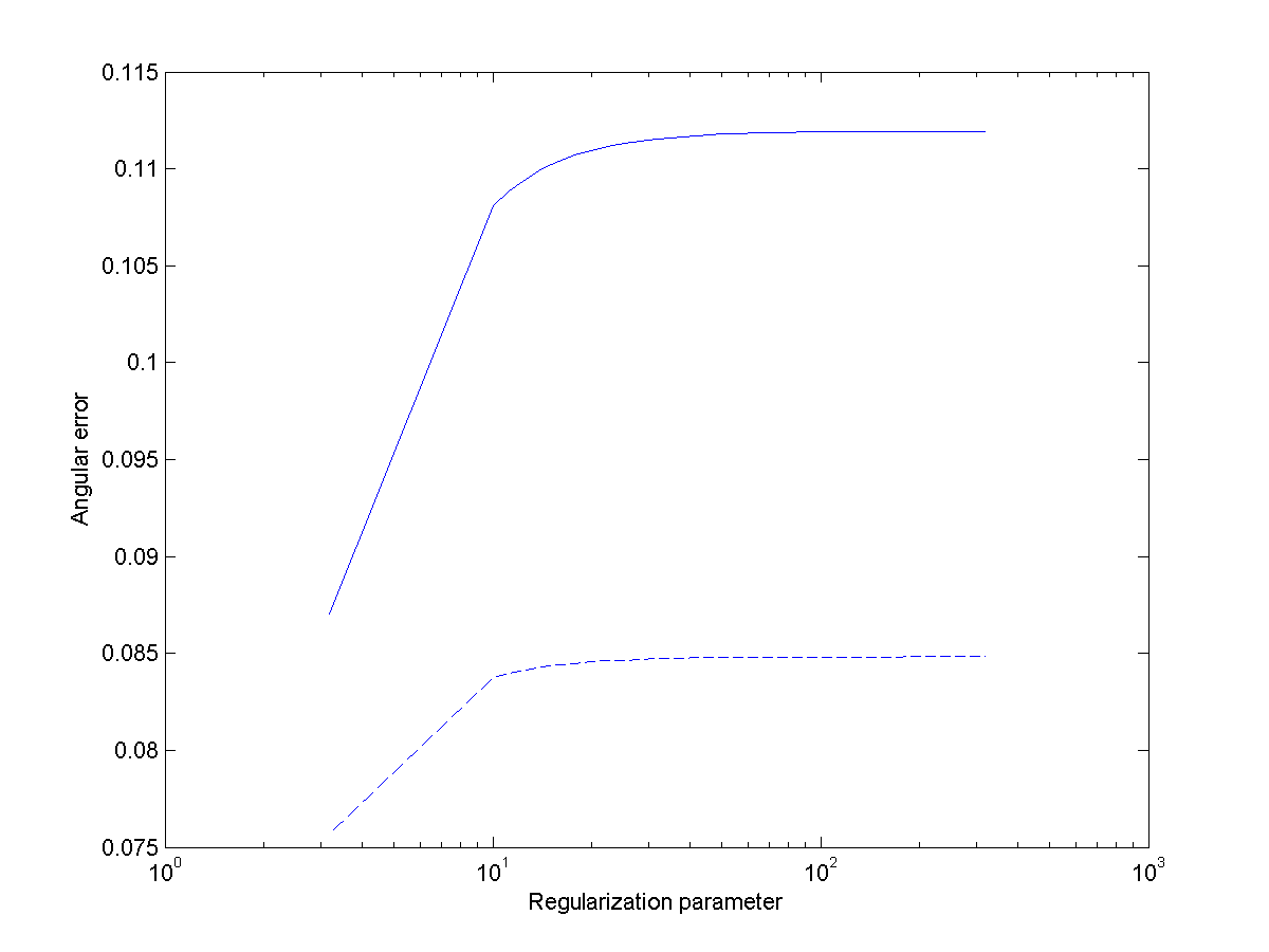
(g) Angular error

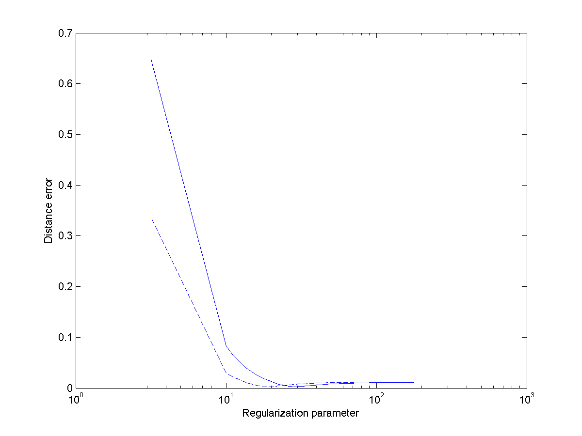
(h) Distance error

Figure 4: (Experiment 3) (c)-(f): Computed vector fields for $\lambda=11.2202$. (g), (h): different error measures for regularization parameters $10^{0.5}\leq\lambda\leq 10^{2.5}$, full line: original data; dashed line: band-limitation texture $\kappa=0.4$

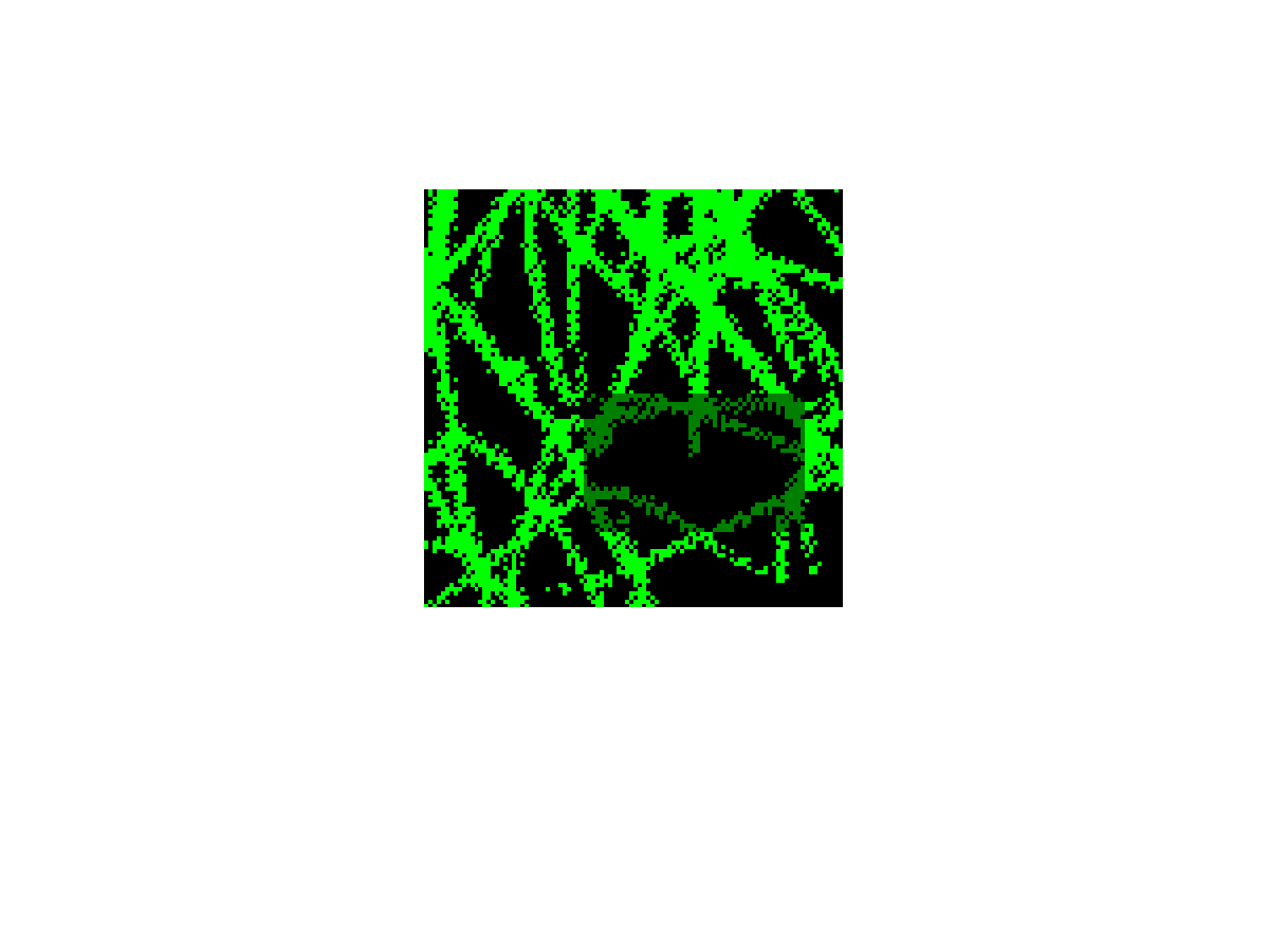
(a) Visualized mask

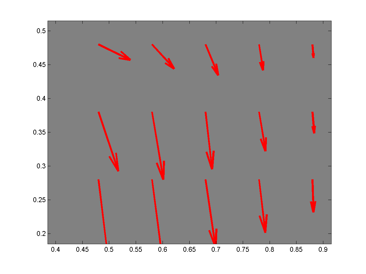
(b) Ground truth

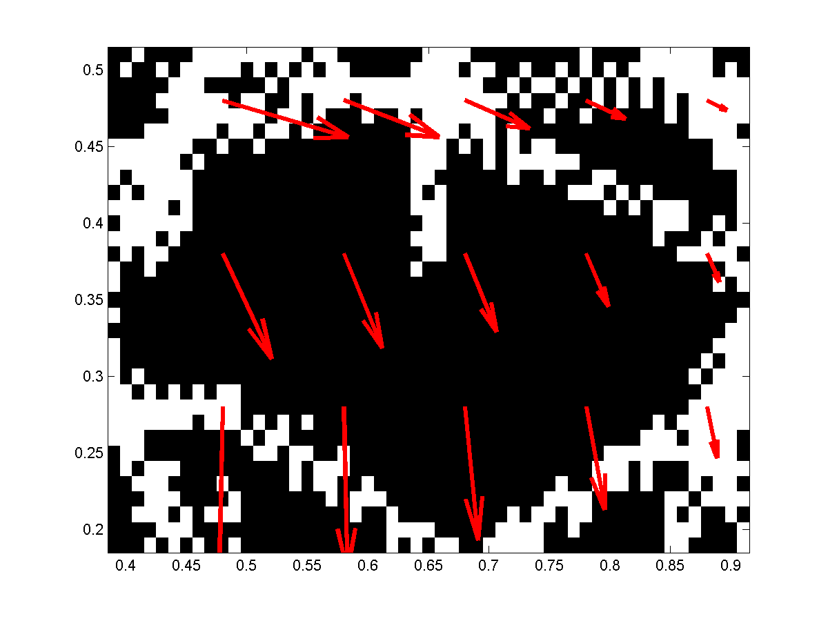
(c) none

(d) Gauss 0.3

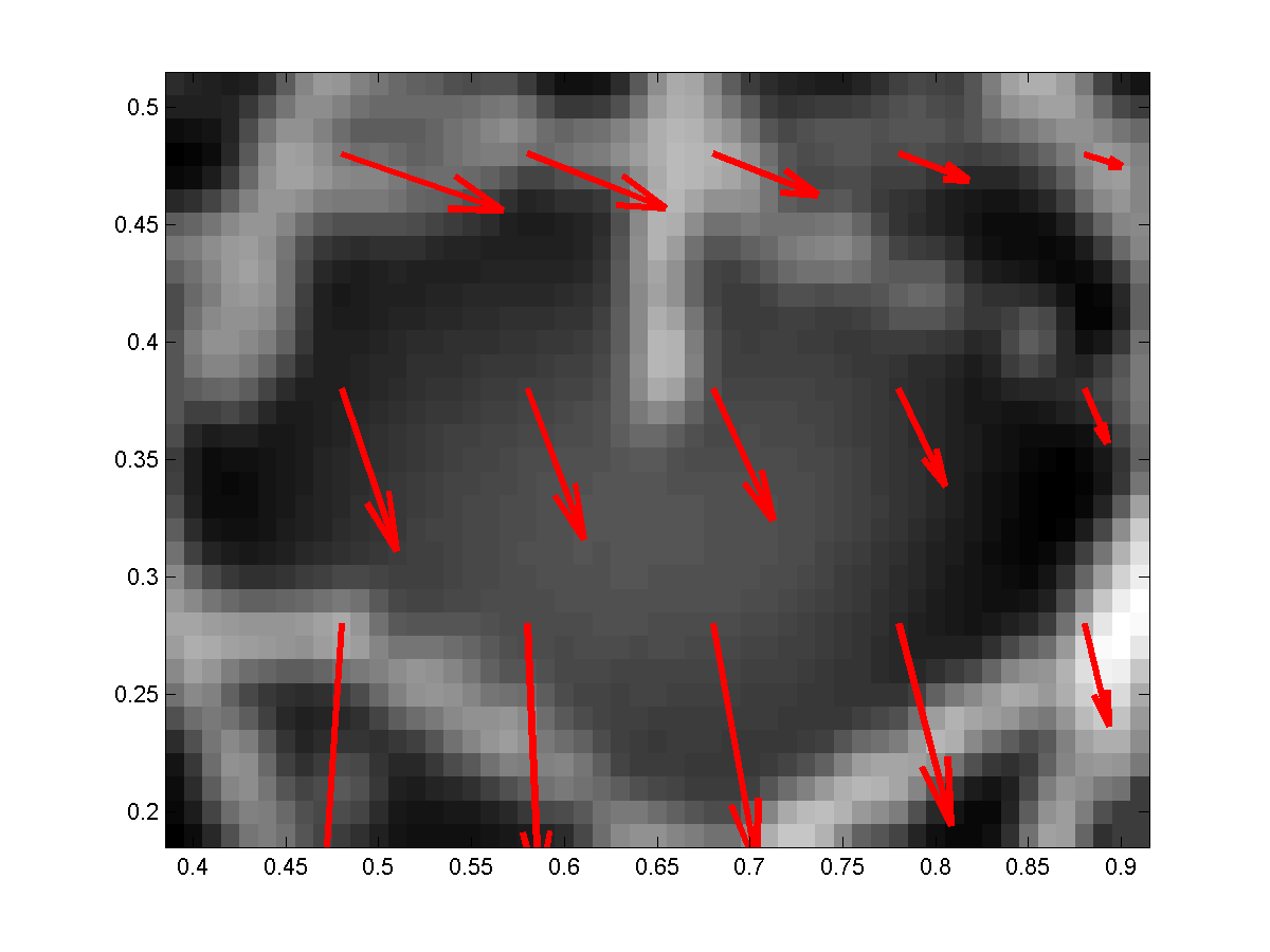
(e) Band 0.4

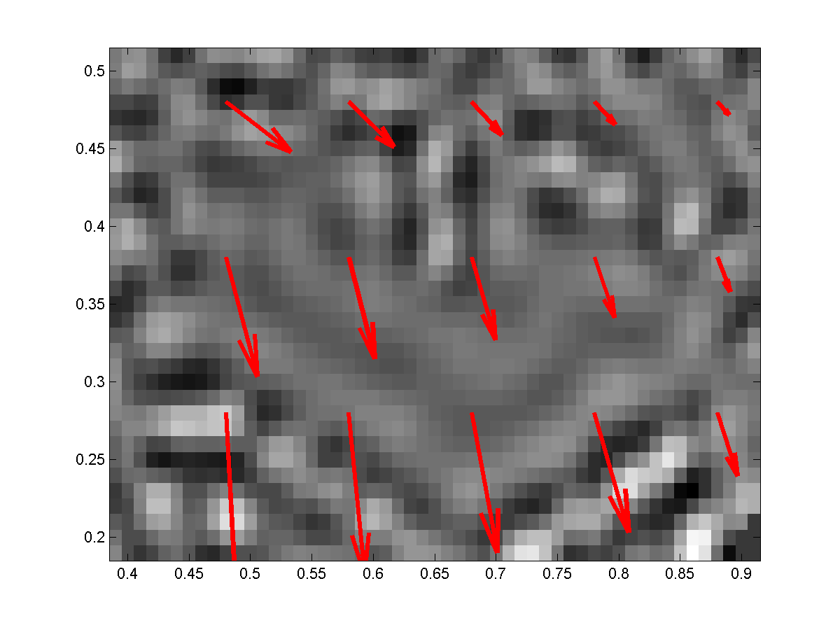
(f) Band 1.8

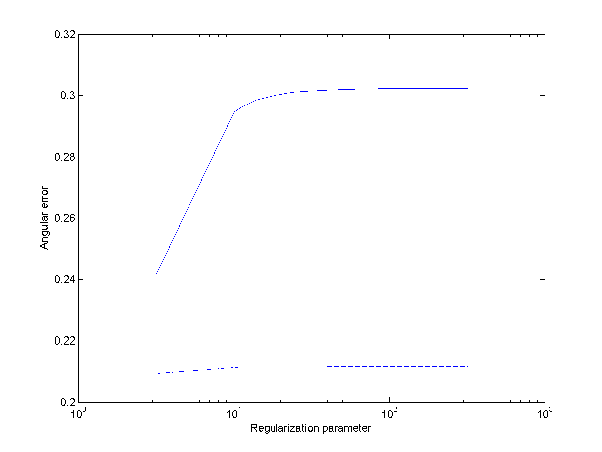
(g) Angular error

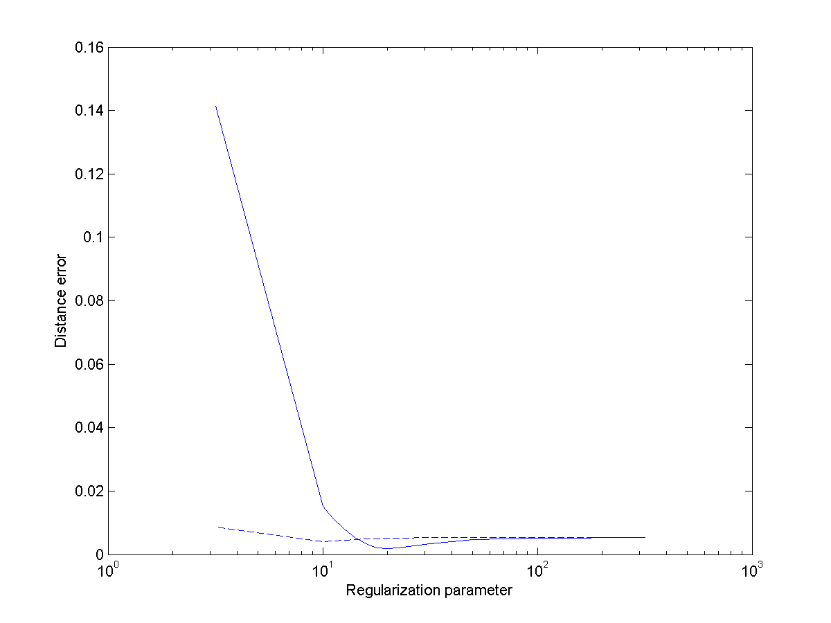
(h) Distance error

Figure 5: (Experiment 4) (c)-(f): Computed vector fields for $\lambda=11.2202$. (g), (h): different error measures for regularization parameters $10^{0.5}\leq\lambda\leq 10^{2.5}$, full line: original data; dashed line: band-limitation texture $\kappa=1.8$

Table 2: Experiments 3 and 4: Error analysis

Texture Mode	AAE	AEEabs	AEErel	Warping
none	0.1089	0.0635	4.7460	0.4382
Gauss 0.3	0.1090	0.0635	4.7465	0.4430
Band 0.4	0.0840	0.0211	1.5807	0.1753
Band 1.8	0.1344	0.0094	0.7024	0.0533

(a) Rigid experiment, $\lambda=11.2202$ (see Figure 4)

Texture Mode	AAE	AEEabs	AEErel	Warping
none	0.2962	0.0112	1.3676	0.2053
Gauss 0.3	0.2956	0.0112	1.3680	0.2127
Band 0.4	0.3251	0.0026	0.3236	0.0191
Band 1.8	0.2115	0.0043	0.5228	0.0216

(b) Non-rigid experiment, $\lambda=11.2202$ (see Figure 5)

Acknowledgements.

We thank Joyce McLaughlin, Paul Beard and Ben Cox for helpful discussions and acknowledge support from the Austrian Science Fund (FWF) in projects S10505-N20 and P26687-N25.

References

- [1] Agranovsky, M., Berenstein, C., Kuchment, P.: Approximation by spherical waves in -spaces. J. Geom. Anal. 6(3), 365–383 (1996)
- [2] Aigner, F., Pallwein, L., Schocke, M., Lebovici, A., Junker, D., Schäfer, G., Pedross, F., Horninger, W., Jaschke, W., Hallpern, E.J., Frauscher, F.: Comparison of real-time sonoelastography with T2-weighted endorectal magnetic resonance imaging for prostate cancer detection. J. Ultrasound Med. 30, 643–649 (2011)
- [3] Arridge, S., Scherzer, O.: Imaging from coupled physics. Inverse Probl. 28(8), 080,201 (2012). DOI 10.1088/0266-5611/28/8/080201. URL http://stacks.iop.org/0266-5611/28/i=8/a=080201
- [4] Beard, P.: Biomedical photoacoustic imaging. Interface Focus 1, 602–631 (2011)
- [5] Biswas, R., Patel, P., Park, D.W., Cichonski, T.J., Richards, M.S., Rubin, J.M., Hamilton, J., Weitzel, W.F.: Venous elastography: validation of a novel high-resolution ultrasound method for measuring vein compliance using finite element analysis. Sem. Dial. 23(1), 105–109 (2010)
- [6] Bohs, L.N., Geiman, B.J., Anderson, M.E., Gebhart, S.C., Trahey, G.E.: Speckle tracking for multi-dimensional flow estimation. Ultrasons 38, 369–375 (2000)
- [7] Bracewell, R.N.: The Fourier Transform and its Applications. McGraw-Hill, New York (1978)
- [8] Doyley, M.M.: Model-based elastography: a survey of approaches to the inverse elasticity problem. Phys. Med. Biol. 57, R35–R73 (2012)
- [9] Dular, P., Geuzaine, C., Henrotte, F., Legros, W.: A general environment for the treatment of discrete problems and its application to the finite element method. IEEE Trans. Magn. 34(5), 3395–3398 (1998)
- [10] Elbau, P., Scherzer, O., Schulze, R.: Reconstruction formulas for photoacoustic sectional imaging. Inverse Probl. 28(4), 045,004 (2012). DOI 10.1088/0266-5611/28/4/045004. URL http://dx.doi.org/10.1088/0266-5611/28/4/045004. Funded by the Austrian Science Fund (FWF) within the FSP S105 - “Photoacoustic Imaging”
- [11] Emelianov, S.Y., Aglyamov, S.R., Shah, J., Sethuraman, S., Scott, W.G., Schmitt, R., Motamedi, M., Karpiouk, A., Oraevsky, A.: Combined ultrasound, optoacoustic and elasticity imaging. Proc. SPIE 5320, 101–12 (2004)
- [12] Evans, L.C.: Partial Differential Equations, Graduate Studies in Mathematics, vol. 19. American Mathematical Society, Providence, RI (1998)
- [13] Fawcett, J.A.: Inversion of -dimensional spherical averages. SIAM J. Appl. Math. 45(2), 336–341 (1985)
- [14] Finch, D., Haltmeier, M., Rakesh: Inversion of spherical means and the wave equation in even dimensions. SIAM J. Appl. Math. 68(2), 392–412 (2007). DOI 10.1137/070682137. URL http://dx.doi.org/10.1137/070682137
- [15] Finch, D., Rakesh: Trace identities for solutions of the wave equation with initial data supported in a ball. Math. Methods Appl. Sci. 28, 1897–1917 (2005)
- [16] Fu, Y.B., Chui, C.K., Teo, C.L., Kobayashi, E.: Motion tracking and strain map computation from quasi-static magnetic resonance elastography. In: B. Fichtinger, A. Martel, T. Peters (eds.) Medical Image Computing and Computer-Assisted Intervention MICCAI 2011, Lecture Notes in Computer Science, vol. 6891, pp. 428–435. Springer (2011)
- [17] Geuzaine, C., Remacle, J.F.: Gmsh: a three-dimensional finite element mesh generator with built-in pre- and post-processing facilities. Numer. Meth. in Engineering 79(11), 1309–1331 (2009)
- [18] Haltmeier, M.: A mollification approach for inverting the spherical mean Radon transform. SIAM J. Appl. Math. 71(5), 1637–1652 (2011)
- [19] Haltmeier, M., Scherzer, O., Zangerl, G.: Influence of detector bandwidth and detector size to the resolution of photoacoustic tomagraphy. In: F. Breitenecker, I. Troch (eds.) Argesim Report no. 35: Proceedings Mathmod 09 Vienna, pp. 1736–1744 (2009)
- [20] Haltmeier, M., Zangerl, G.: Spatial resolution in photoacoustic tomography: effects of detector size and detector bandwidth. Inverse Probl. 26(12), 125,002 (2010). DOI 10.1088/0266-5611/26/12/125002. URL http://dx.doi.org/10.1088/0266-5611/26/12/125002
- [21] Helgason, S.: Integral Geometry and Radon Transform. Springer, New York, NY (2011)
- [22] Horn, B.K.P., Schunck, B.G.: Determining optical flow. Artificial Intelligence 17, 185–203 (1981)
- [23] J., L.C.M., Kybic, J., Desco, M., Santos, A., Sühling, M., Hunziker, P., Unser, M.: Spatio-temporal nonrigid registration for ultrasound cardiac motion estimation. IEEE Trans. Med. Imag. 24(9), 1113–1126 (2005)
- [24] Kuchment, P., Kunyansky, L.: Mathematics of thermoacoustic tomography. European J. Appl. Math. 19, 191–224 (2008). DOI 10.1017/S0956792508007353
- [25] Lerner, R.M., Parker, K.J., Holen, J., Gramiak, R., Waag, R.C.: Sono-elasticity: medical elasticity images derived from ultrasound signals in mechanically vibrated targets. Ann. Comb. 16, 317–327 (1988)
- [26] Li, C., Wang, L.V.: Photoacoustic tomography and sensing in biomedicine. Phys. Med. Biol. 54, R59–R97 (2009). DOI 10.1088/0031-9155/54/19/R01
- [27] Li, L., Wang, L.V.: Speckle in photoacoustic tomography. Proc. SPIE 6095, 60,860Y (2006). DOI doi:10.1117/12.646357
- [28] Manduca, A., Oliphant, T.E., Dresner, M.A., Mahowald, J.L., Kruse, S.A., Amromin, E., Felmlee, J.P., Greenleaf, J.F., Ehman, R.L.: Magnetic resonance elastography: Non-invasive mapping of tissue elasticity. Med. Image Anal. 5, 237–354 (2001)
- [29] Muthupillai, R., Lomas, D.J., Rossman, P.J., Greenleaf, J.F., Manduca, A., Ehman, R.L.: Magnetic resonance elastography by direct visualization of propagating acoustic strain waves. Science 269, 1854–1857 (1995)
- [30] Nahas, A., Bauer, M., Roux, S., Boccara, A.C.: 3D static elastography at the micrometer scale using Full Field OCT. Biomed. Opt. Express 4(10), 2138–2149 (2013)
- [31] Natterer, F.: The mathematics of computerized tomography, Classics in Applied Mathematics, vol. 32. Society for Industrial and Applied Mathematics (SIAM), Philadelphia, PA (2001). Reprint of the 1986 original
- [32] Nilsson, S.: Application of fast backprojection techniques for some inverse problems of integral geometry. Ph.D. thesis, Linköping University, Dept. of Mathematics (1997)
- [33] Norton, S.J.: Reconstruction of a two-dimensional reflecting medium over a circular domain: Exact solution. J. Acoust. Soc. Amer. 67(4), 1266–1273 (1980)
- [34] Norton, S.J., Linzer, M.: Ultrasonic reflectivity imaging in three dimensions: Exact inverse scattering solutions for plane, cylindrical and spherical apertures. IEEE Trans. Biomed. Eng. 28(2), 202–220 (1981)
- [35] Nuster, R., Slezak, P., Paltauf, G.: Imaging of blood vessels with CCD-camera based three-dimensional photoacoustic tomography. Proc. SPIE 8943, 894,357 (2014)
- [36] Oberhettinger, F.: Tables of Fourier transforms and Fourier transforms of distributions. Springer-Verlag, Berlin (1990). Translated and revised from the German
- [37] Ophir, J., Cespedes, I., Ponnekanti, H., Yazdi, Y., Li, X.: Elastography: a quantitative method for imaging the elasticity of biological tissues. Ultrason. Imaging 13, 111–134 (1991)
- [38] Palamodov, V.P.: Reconstructive Integral Geometry, Monographs in Mathematics, vol. 98. Birkhäuser Verlag, Basel (2004)
- [39] Pan, X., Gao, J., Tao, S., Liu, K., Bai, J., Luo, J.: A two-step optical flow method for strain estimation in elastography: simulation and phantom study. Ultrasons 54, 990–996 (2014)
- [40] Parker, K.J., Doyley, M.M., Rubens, D.J.: Imaging the elastic properties of tissue: the 20 year perspective. Phys. Med. Biol. 56, R1–R29 (2011)
- [41] Prasad, P.R., Bhattacharya, S.: Improvements in speckle tracking algorithms for vibrational analysis using optical coherence tomography. J. Biomed. Opt. 18(4), 18 (2014)
- [42] Prince, J.L., McVeigh, E.R.: Motion estimation from tagged MR image sequences. IEEE Trans. Med. Imag. 11(2), 238–249 (1992)
- [43] Ramm, A.: Inversion of the backscattering data and a problem of integral geometry. Phys. Lett. A 113, 172–176 (1985)
- [44] Revell, J., Mirmehdi, M., McNally, D.: Computer vision elastography: speckle adaptive motion estimation for elastography using ultrasound sequences. IEEE Trans. Med. Imag. 24(6), 755–766 (2005)
- [45] Scherzer, O., Grasmair, M., Grossauer, H., Haltmeier, M., Lenzen, F.: Variational methods in imaging, Applied Mathematical Sciences, vol. 167. Springer, New York (2009). DOI 10.1007/978-0-387-69277-7. URL http://dx.doi.org/10.1007/978-0-387-69277-7
- [46] Schmitt, J.M.: OCT elastography: imaging microscopic deformation and strain of tissue. Opt. Express 3(6), 199–211 (1998)
- [47] Solmon, D.C.: Asymptotic formulas for the dual radon transform and applications. Math. Z. 195(3), 321–343 (1987)
- [48] Sun, C., Standish, B., Yang, V.X.D.: Optical coherence elastography, current status and future applications. J. Biomed. Opt. 16(4), 043,001 (2011)
- [49] Treeby, B.E., Cox, B.T.: K-Wave: MATLAB toolbox for the simulation and reconstruction of photoacoustic wace fields. J. Biomed. Opt. 15, 021,314 (2010)
- [50] Wang, H.J., Changchien, C.S., Hung, C.H., Eng, E.L., Tung, W.C., Kee, K.M., Chen, C.H., Hu, T.H., Lee, C.M., Lu, S.N.: Fibroscan and ultrasonography in the prediction of hepatic fobrosis in patients with chronic viral hepatitis. J. Gastroenterol. 44, 439–436 (2009)
- [51] Washington, C.W., Miga, M.I.: Modality independent elastography (MIE): a new approach to elasticity imaging. IEEE Trans. Med. Imag. 23(9), 1117–1128 (2004)
- [52] Wejcinski, S., Farrokh, A., Weber, S., Thomas, A., Fischer, T., Slowinski, T., Schmidt, W., Degenhardt, F.: Multicenter study of ultrasound real-time tissue elastography in 779 cases for the assessment of breast lesions: improved diagnostic performance by combining the BI-RADS®-US classification system with sonoelastography. Ultraschall Med. 31, 484–491 (2010)
- [53] Woodrum, D.A., Romano, A.J., Lerman, A., Pandya, U.H., Brosh, D., Rossman, P.J., Lerman, L.O., Ehman, R.L.: Vascular wall elasticity measurement by magnetic resonance imaging. Magn. Reson. Med. 56, 593–600 (2006)
- [54] Zakaria, T., Qin, Z., Maurice, R.L.: Optical flow-based B-mode elastography: application in the hypertensitive rat carotid. IEEE Trans. Med. Imag. 29(2), 570–578 (2010)