Analysis of resonant inelastic x-ray scattering from Sr₂IrO₄ in an itinerant-electron approach

Abstract

We analyze the resonant x-ray scattering (RIXS) spectra from Sr₂IrO₄ in an itinerant electron approach. Employing a multi-orbital tight-binding model on the square lattice, we calculate the one-electron energy band within the Hartree-Fock approximation, which leads to an antiferromagnetic ground state. We then evaluate the two-particle Green’s functions for the particle-hole pair excitations within the random phase approximation, which are connected to the RIXS spectra within the fast collision approximation. The calculated RIXS spectra exhibit two-peak structure with slightly different energies in the low-energy region, which are originated from the bound states in the two-particle Green’s function. They may be interpreted as the split modes of magnon. We also obtain several $\delta$-function peaks, which arise from the bound states around the bottom of energy continuum. They may be called as the exciton modes. These characteristics are in qualitative agreement with the RIXS experiment, demonstrating that the weak coupling theory could explain both the magnon and the exciton peaks in the RIXS spectra on an equal footing.

I Introduction

Strong synchrotron sources have been rapidly developing, and resonant inelastic x-ray scattering (RIXS) has become a powerful tool to probe elementary excitations in solids Ament et al. (2011a); Ishii et al. (2013). Both the $K$- and $L$-edge resonances are utilized in transition-metal compounds. On the $K$ edge resonance, the $1s$ core-electron is prompted to empty $p$-symmetric states by absorbing photon, then the photo-excited electron is recombined with the core hole by emitting photon. In this process, charge excitations are created to screen the core-hole potential in the intermediate state. Note that two magnons could also be created in magnetic systems Nagao and Igarashi (2007); van den Brink (2007); Hill et al. (2008); Forte et al. (2008), since the exchange coupling is modified around the core-hole site in the presence of the core-hole potential.

On the $L$-edge resonance, on the other hand, the $2p$ core-electron is prompted to empty $d$-symmetric states by absorbing photon, then an electron occupied on the $d$-symmetric state is combined with the core hole by emitting photon. Since the electron combined with the core hole is not necessarily the same as the photo-excited electron, the particle-hole pair excitations could be directly created in the $d$-symmetric states in addition to the screening effect of the core-hole potential in the intermediate state. Note that the $2p$-core states are split into two well-separated levels with the total angular momentum $j_{c}=1/2$ and $j_{c}=3/2$ due to the strong spin-orbit interaction (SOI). The corresponding $L$-edges are discriminated as the $L_{2}$ and $L_{3}$-edges, respectively. Owing to this split, the single spin-flip excitations could be created. Actually, the spectral peaks as a function of energy loss are found to follow the dispersion of spin waves in the Heisenberg model with changing momentum transfer in undoped cuprates Braicovich et al. (2009, 2010); Guarise et al. (2010). Such $L$-edge RIXS spectra have been analyzed on the spin model within the fast collision approximation (FCA), which is justified when the core-hole life-time broadening width is larger than the concerned excitation energy Ament et al. (2007, 2009); Haverkort (2010). Although only the one-magnon excitations could be created within the FCA, the experimental energy profile shows asymmetric shape Braicovich et al. (2009, 2010); Guarise et al. (2010), indicating that two-magnon excitations are involved in addition to the one-magnon excitations. An analysis going beyond the FCA has been carried out to explain the asymmetrical profile in quantitative agreement with the experiment Igarashi and Nagao (2012a, b); Nagao and Igarashi (2012).

Recently, RIXS experiments have been carried out at the Ir L₃ edge in Sr₂IrO₄ Ishii et al. (2011); Kim et al. (2012a). This material shows the antiferromagnetism at low temperatures below $\sim$ 230 K Crawford et al. (1994); Cao et al. (1998); Moon et al. (2006). Its ordering is concerned with the spin-orbital coupled isospin $j_{\rm eff}=1/2$, since the SOI is large on the $5d$ states of Ir Jackeli and Khaliullin (2009). The low-energy peak behaves like the one-magnon peak in undoped cuprates Kim et al. (2012a), while other peaks emerge around $\omega\sim 0.5$ eV with substantial weights as a function of energy loss $\omega$. The RIXS spectra have been analyzed within the FCA on the basis of the localized electron model Ament et al. (2011b); Igarashi and Nagao (2014a). Note that the FCA is expected to work well for this material, since the $2p$-core hole has the life-time broadening width as large as $2.5-3.5$ eV Krause and Oliver (1979), which is much larger than the concerned excitation energies. The low-energy peak has been interpreted as the magnetic excitation (magnon) in the isospin space $j_{\rm eff}=1/2$, while the peak around $\omega\sim 0.5$ eV as the excitation (exciton) from the $j_{\rm eff}=3/2$ manifold to $j_{\rm eff}=1/2$ manifoldKatukuri et al. (2012). Recently, the magnon mode has been predicted to be split into two modes due to the interplay between Hund’s coupling and the SOI, and a detailed analysis of the magnon peak has been made with taking account of the mode splitting Igarashi and Nagao (2013a, 2014a).

Although the localized electron model has been successful in analyzing the RIXS spectra, there remain issues that the itineracy of the electrons might play a key role to elucidate the physical features of Sr₂IrO₄. For instance, it has been argued whether the system behaves like the Mott insulator or the band insulator Arita et al. (2012); Moser et al. (2014). It is also established that the isotropic Heisenberg model can reproduce the magnon dispersion only when it includes the second and third nearest neighbor exchange coupling in addition to the first nearest neighbor exchange coupling Kim et al. (2012b). Such observations naturally prompt us to investigate the material in the itinerant electron approach and several attempts have been carried out to study its electronic structure. The band structure calculation has been carried out within the local density approximation augmented by the Coulomb interaction (LDA+U), having led to the antiferromagnetic ordering and the associated energy gap in the one-electron energy band Kim et al. (2008). The electron correlation effects have been taken into account by the variational method Watanabe et al. (2010), as well as by the dynamical mean field theory Arita et al. (2012). Recently, excitation spectra have been investigated by calculating the spectral function of the two-particle Green’s function for particle-hole pair excitations within the Hartree-Fock approximation (HFA) and the random phase approximation (RPA) Igarashi and Nagao (2014b), having led that they are composed of magnons and excitons. However, a direct comparison between the spectral function and the RIXS spectrum cannot be allowed, since the former is different from the RIXS spectra due to the second-order optical process.

The purpose of this paper is to analyze the RIXS spectra with an argument based on an itinerant electron picture. Introducing the multi-orbital tight-binding model, we calculate the one-electron energy band within the HFA, where the antiferromagnetic ground state is realized. Then, on this ground state, we calculate the two-particle Green’s function for the particle-hole pair excitations within the RPA. Magnons appear as bound states below the energy continuum, and are split into two modes. Other several bound states emerge around the bottom of the energy continuum Com . These together with the continuum states (often containing resonant modes) may constitute exciton modes.

The spectral function of the two-particle Green’s function are related with the RIXS spectra within the FCA, which is known to work well for the RIXS spectra in Sr₂IrO₄. For magnons split into two modes, the two-peak structures are found with significant momentum dependence of intensities. The splitting of the magnon modes, however, has not been confirmed yet by RIXS experiments, probably because the experimental energy resolution is as large as $40$ meV. Furthermore, sharp exciton peaks emerge with their intensities larger than the magnon intensities, being separated from the magnon peaks, in consistent with the RIXS experiment. Thus it is demonstrated that the weak coupling approach of the HFA and RPA could explain both the magnon and the exciton peaks in the RIXS spectra on an equal footing, providing a good starting point of taking account of electron correlations.

The present paper is organized as follows. In Sec. II, we introduce a multi-orbital tight-binding model, and study the electronic structure within the HFA. In Sec. III, we describe the dipole process, and calculate the absorption coefficient at the $L$ edge. In Sec. IV, we derive the formula for the RIXS spectra within the FCA. In Sec. V, comparisons are made between the calculated and experimental RIXS spectra. Section VI is devoted to the concluding remarks.

II Electronic structure

II.1 Model Hamiltonian

Transition metal oxide Sr₂IrO₄ with the K₂NiF₄-type structure is composed of IrO₂ layer separated by Sr-O layer Crawford et al. (1994). Since the crystal field energy of the $e_{g}$ orbitals is about 2 eV higher than that of the $t_{2g}$ orbitals, we consider only $t_{2g}$ orbitals with five electrons occupying in each Ir atom. Since the oxygen octahedra surrounding an Ir atom are rotated about the crystallographic $c$ axis by about 11^∘ Watanabe et al. (2010); Wang and Senthil (2011), the $t_{2g}$ states are defined in the local coordinate frames rotated in accordance with the rotation of octahedra. For simplicity, disregarded is the fact that the degenerate $t_{2g}$ levels are split by the tetragonal crystal field due to the rotation and distortion of IrO₆ octahedra. Then, we start from the multi-orbital Hubbard model on the square lattice in the local coordinate frames,

$$H=H_{\rm kin}+H_{\rm SO}+H_{\rm I},$$ (1)

where $H_{\rm kin}$, $H_{\rm SO}$, and $H_{\rm I}$ are described by the annihilation ($d_{in\sigma}$) and creation ($d_{in\sigma}^{\dagger}$) operators of an electron with orbital $n$ ($=yz,zx,xy$) and spin $\sigma$ at the Ir site $i$ as follows.

$$H_{\rm kin} = \sum_{\left\langle i,i^{\prime}\right\rangle}\sum_{n,n^{\prime},\sigma}t_{in,i^{\prime}n^{\prime}}d_{in\sigma}^{\dagger}d_{i^{\prime}n^{\prime}\sigma}+{\rm H.c.},$$ (2)

$$H_{\rm SO} = \zeta_{\rm SO}\sum_{i}\sum_{n,n^{\prime},\sigma,\sigma^{\prime}}d_{in\sigma}^{\dagger}({\bf L})_{nn^{\prime}}\cdot({\bf S})_{\sigma\sigma^{\prime}}d_{in^{\prime}\sigma^{\prime}},$$ (3)

$$H_{\rm I} = U\sum_{i,n}n_{in\uparrow}n_{in\downarrow}$$

$$+ \sum_{i,n<n^{\prime},\sigma}[U^{\prime}n_{in\sigma}n_{in^{\prime}-\sigma}+(U^{\prime}-J)n_{in\sigma}n_{in^{\prime}\sigma}]$$

$$+ J\sum_{i,n\neq n^{\prime}}(d_{in\uparrow}^{\dagger}d_{in^{\prime}\downarrow}^{\dagger}d_{in\downarrow}d_{in^{\prime}\uparrow}+d_{in\uparrow}^{\dagger}d_{in\downarrow}^{\dagger}d_{in^{\prime}\downarrow}d_{in^{\prime}\uparrow}).$$

The inter-site interaction $H_{\rm kin}$ stands for the kinetic energy. The transfer integral $t_{in,i^{\prime}n^{\prime}}$ exhibits a highly anisotropic nature. An electron on the $xy$ orbital could transfer to the $xy$ orbital in the nearest neighbor sites through the intervening O $2p$ orbitals, while an electron on the $yz$($zx$) orbital could transfer to the $yz$($zx$) orbital in the nearest-neighbor sites only along the $y$($x$) direction. The none-zero values of $t_{in,i^{\prime}n^{\prime}}$’s are assumed to be the same and denoted as $t_{1}$. The SOI of $5d$ electrons is denoted as $H_{\rm SO}$ with ${\bf L}$ and ${\bf S}$ denoting the orbital and spin angular momentum operators. The $H_{\rm I}$ represents the Coulomb interaction between electrons with $\nu=(n,\sigma)$. Parameters satisfy $U=U^{\prime}+2J$ Kanamori (1963). We use the values $U=1.4$ eV, and $J/U=0.15$ in the following calculation. As regards the transfer integral $t_{1}$ and the SOI parameter $\zeta_{\rm SO}$, we consider two typical parameter sets; one is that $\zeta_{\rm SO}=0.36$ eV, $t_{1}=0.36$ eV (Case A), and another is that $\zeta_{\rm SO}=0.45$ eV, $t_{1}=0.25$ eV (Case B). The values in Case A are the same as in [Watanabe et al., 2013], and give the one-electron band width consistent with the band calculation based on the local density approximationKim et al. (2008); Igarashi and Nagao (2014b). The smaller value of $t_{1}$ in Case B may lead to the larger energy gap in the one-electron band. Note that the smaller values of $t_{1}$ around 0.1-0.2 eV have been estimated on the basis of a localized picturePerkins et al. (2014).

II.2 Hartree-Fock Approximation

A unit cell $j$ contains two atoms at ${\bf r}_{j}$ and at ${\bf r}_{j}+{\bf a}$, where ${\bf a}=(a,0)$ with $a$ a nearest neighbor distance. We introduce the Fourier transform of annihilation operator with the wave vector ${\bf k}$ in the magnetic Brillouin zone (MBZ), which is defined as the half of the first Brillouin zone:

$$d_{\lambda n\sigma}({\bf k})=\sqrt{\frac{2}{N}}\sum_{j}d_{j^{\prime}n\sigma}\textrm{e}^{-i{\bf k}\cdot{\bf r}_{j}},$$ (5)

where $j$ runs over unit cells and $N/2$ stands for the number of the unit cells. We assign $\lambda=1$ and $2$ for the A and B sublattices, respectively. The index $j^{\prime}$ specifies the site within the $j$-th unit cell as $\textbf{r}_{j^{\prime}}={\bf r}_{j}$ and ${\bf r}_{j}+{\bf a}$ for $\lambda=1$ and $2$, respectively. Then, the one-electron energy $H_{0}\equiv H_{\rm kin}+H_{\rm SO}$ may be rewritten as

$$H_{0}=\sum_{{\bf k}\xi\xi^{\prime}}d_{\xi}^{\dagger}({\bf k})\left[\hat{H}_{0}({\bf k})\right]_{\xi,\xi^{\prime}}d_{\xi^{\prime}}({\bf k}),$$ (6)

with abbreviations $\xi=(\lambda,n,\sigma)$ and $\xi^{\prime}=(\lambda^{\prime},n^{\prime},\sigma^{\prime})$.

Arranging $\xi$ in order $(1,yz,\uparrow)$, $(1,zx,\uparrow)$, $(1,xy,\uparrow)$, $(1,yz,\downarrow)$, $(1,zx,\downarrow)$, $(1,xy,\downarrow)$, $(2,yz,\uparrow)$, $(2,zx,\uparrow)$, $(2,xy,\uparrow)$, $(2,yz,\downarrow)$, $(2,zx,\downarrow)$, $(2,xy,\downarrow)$, we have $\hat{H}_{0}({\bf k})$ in a block form,

$$\hat{H}_{0}({\bf k})=\left(\begin{array}[]{cc}\hat{H}_{\rm AA}^{0}({\bf k})&\hat{H}_{\rm AB}^{0}({\bf k})\\ \hat{H}_{\rm BA}^{0}({\bf k})&\hat{H}_{\rm BB}^{0}({\bf k})\end{array}\right),$$ (7)

where

$$\hat{H}_{\rm AA}^{0}({\bf k})=\hat{H}_{\rm BB}^{0}({\bf k})=\frac{\zeta_{\rm SO}}{2}\left(\begin{array}[]{cccccc}0&i&0&0&0&-1\\ -i&0&0&0&0&i\\ 0&0&0&1&-i&0\\ 0&0&1&0&-i&0\\ 0&0&i&i&0&0\\ -1&-i&0&0&0&0\end{array}\right),$$ (14)

(15)

$$\hat{H}_{\rm AB}^{0}({\bf k})=[\hat{H}_{\rm BA}^{0}({\bf k})]^{\star}$$

$$=\left(\begin{array}[]{cccccc}t_{1}({\bf k})&0&0&0&0&0\\ 0&t_{2}({\bf k})&0&0&0&0\\ 0&0&t_{3}({\bf k})&0&0&0\\ 0&0&0&t_{1}({\bf k})&0&0\\ 0&0&0&0&t_{2}({\bf k})&0\\ 0&0&0&0&0&t_{3}({\bf k})\end{array}\right).$$ (22)

Here the dispersion may be expressed as

$$t_{n}(\textbf{k})=-2t_{1}{\rm e}^{-ik_{x}}\times\left\{\begin{array}[]{lcl}\cos k_{y},&\textrm{for}&n=1\\ \cos k_{x},&\textrm{for}&n=2\\ (\cos k_{x}+\cos k_{y}),&\textrm{for}&n=3\\ \end{array}\right.,$$ (23)

where ${\bf k}$ is measured in units of $1/a$.

We follow the conventional procedure of the HFA as explained in Ref. Igarashi and Nagao, 2013b. Rewriting $H_{\rm I}=\frac{1}{2}\sum_{i}\sum_{\nu_{1},\nu_{2},\nu_{3},\nu_{4}}g(\nu_{1}\nu_{2};\nu_{3}\nu_{4})d_{i\nu_{1}}^{\dagger}d_{i\nu_{2}}^{\dagger}d_{i\nu_{4}}d_{i\nu_{3}}$, we replace $H_{\rm I}$ by

$$H_{\rm I}^{\rm HF}=\frac{1}{2}\sum_{j}\sum_{\xi_{1},\xi_{2},\xi_{3},\xi_{4}}\Gamma^{(0)}(\xi_{1}\xi_{2};\xi_{3}\xi_{4})\langle d_{j\xi_{2}}^{\dagger}d_{j\xi_{4}}\rangle d_{j\xi_{1}}d_{j\xi_{3}},$$ (24)

where $\Gamma^{(0)}$ is the antisymmetric vertex function,

$$\Gamma^{(0)}(\xi_{1}\xi_{2};\xi_{3}\xi_{4})=g(\xi_{1}\xi_{2};\xi_{3}\xi_{4})-g(\xi_{1}\xi_{2};\xi_{4}\xi_{3}),$$ (25)

with $\xi=(\lambda,\nu)$. Here, $d_{j\xi}=d_{j(\lambda\nu)}$ denotes the annihilation operator of the $d$ electron with $\nu$ spin-orbital state at the site belonging to the sublattice $\lambda$ in the $j$-th unit cell. Then, we introduce the single-particle Green’s function in a matrix form with $12\times 12$ dimensions,

$$\left[\hat{G}({\bf k},\omega)\right]_{\xi,\xi^{\prime}}=-i\int\langle T[d_{\xi}({\bf k},t)d_{\xi^{\prime}}^{\dagger}({\bf k},0)]\rangle{\rm e}^{i\omega t}{\rm d}t,$$ (26)

where $T$ is the time ordering operator, and $\langle X\rangle$ denotes the ground-state average of operator $X$. The Green’s function is obtained by solving the equations of motion, resulting in

$$[\hat{G}({\bf k},\omega)]_{\xi,\xi^{\prime}}=\sum_{\ell}\frac{[\hat{U}({\bf k})]_{\xi,\ell}[\hat{U}({\bf k})^{-1}]_{\ell,\xi^{\prime}}}{\omega-E_{\ell}({\bf k})+i\epsilon{\rm sgn}[E_{\ell}({\bf k})]},$$ (27)

where ${\rm sgn}[A]$ stands for a sign of quantity $A$ and $\delta$ denotes a positive convergent factor. The $\ell$-th energy eigenvalue within the HFA is written as $E_{\ell}({\bf k})$ measured from the chemical potential. The definition of the unitary matrix $\hat{U}({\bf k})$ is found in Ref. Igarashi and Nagao, 2013b. The Green’s function contains the expectation values of the electron density operator on the ground state, which are self-consistently determined from

$$\langle a_{\xi}^{\dagger}a_{\xi^{\prime}}\rangle=\frac{2}{N}\sum_{{\bf k}}\int[-i\hat{G}({\bf k},\omega)]_{\xi,\xi^{\prime}}{\rm e}^{i\omega 0^{+}}\frac{{\rm d}\omega}{2\pi}.$$ (28)

This equation is solved by iteration with summing over ${\bf k}$ by dividing the MBZ into $100\times 100$ meshes. We obtain a self-consistent solution of the antiferromagnetic order with the staggered magnetic moment along the $x$ axis as the ground state, which is consistent with the magnetic measurements Crawford et al. (1994); Cao et al. (1998). Both the orbital and the spin moments are induced due to the strong SOI; $\langle S_{x}\rangle=\pm 0.112$ (Case A) and $\pm 0.143$ (Case B), while $\langle L_{x}\rangle=\pm 0.435$ (Case A) and $\pm 0.551$ (Case B). The antiferromagnetic order in the local coordinate frames indicates that a weak ferromagnetic moment is induced in the coordinate frame fixed to the crystal axes. The one-electron energy has a finite gap due to the antiferromgnatic order.

III Dipole transition and absorption spectra

III.1 Dipole transition

For the interaction between photon and matter, we consider the dipole transition at the $L$ edge, where the $2p$ core-electron is excited to the $5d$ states by absorbing photon (and the reverse process). This process may be described by the interaction

$$H_{x} = \sum_{\lambda,n,\sigma,j_{c},m,\alpha}w(n\sigma;j_{c}m;\alpha)$$

$$\times \sum_{\bf{k},\bf{q}}d_{\lambda n\sigma}^{\dagger}({\bf k+q})p_{\lambda j_{c}m}({\bf k})c_{\alpha}({\bf q})v(\lambda,{\bf q})+{\rm H.c.},$$

where $c_{\alpha}({\bf q})$ is the annihilation operator of photon with momentum ${\bf q}$ and polarization $\alpha$. The $p_{\lambda j_{c}m}({\bf k})$ is the annihilation operator of core electron belonging to the $\lambda$ site with wave vector ${\bf k}$ and the angular momentum $j_{c}=3/2$ and $1/2$ and magnetic quantum number $m$. The $v(\lambda,{\bf q})$ stands for the extra phase on the B sites, which is explicitly defined as

$$v(\lambda,{\bf q})=\delta_{\lambda,1}+\delta_{\lambda,2}{\rm e}^{iq_{x}}.$$ (30)

Note that, when ${\bf k+q}$ lies outside the first MBZ, it is reduced back to the inside of the first MBZ by a reciprocal lattice vector in the reduced zone scheme. The $w(n\sigma;j_{c}m;\alpha)$ represents the matrix elements of the $2p\to 5d$ transition. Table I lists the values for $\alpha=x$, $y$, $z$ corresponding to the polarization directing to the $x$, $y$, $z$ axes.

Table 1: $w(n\sigma;j_{c}m;\alpha)$ within $t_{2g}$ basis with $j_{c}=\frac{3}{2}$ and $\frac{1}{2}$.

		$j_{c}=\frac{3}{2}$				$j_{c}=\frac{1}{2}$
$\alpha$	$(n\sigma)\setminus m$	$\frac{3}{2}$	$\frac{1}{2}$	$-\frac{1}{2}$	$-\frac{3}{2}$	$\frac{1}{2}$	$-\frac{1}{2}$
$x$	$(zx\uparrow)$	0	$\frac{\sqrt{2}}{\sqrt{15}}$	0	0	$\frac{1}{\sqrt{15}}$	0
	$(zx\downarrow)$	0	0	$\frac{\sqrt{2}}{\sqrt{15}}$	0	0	$-\frac{1}{\sqrt{15}}$
	$(xy\uparrow)$	$-\frac{i}{\sqrt{10}}$	0	$-\frac{i}{\sqrt{30}}$	0	0	$-\frac{i}{\sqrt{15}}$
	$(xy\downarrow)$	0	$-\frac{i}{\sqrt{30}}$	0	$-\frac{i}{\sqrt{10}}$	$\frac{i}{\sqrt{15}}$	0
$y$	$(yz\uparrow)$	0	$\frac{\sqrt{2}}{\sqrt{15}}$	0	0	$\frac{1}{\sqrt{15}}$	0
	$(yz\downarrow)$	0	0	$\frac{\sqrt{2}}{\sqrt{15}}$	0	0	$-\frac{1}{\sqrt{15}}$
	$(xy\uparrow)$	$-\frac{1}{\sqrt{10}}$	0	$\frac{1}{\sqrt{30}}$	0	0	$\frac{1}{\sqrt{15}}$
	$(xy\downarrow)$	0	$-\frac{1}{\sqrt{30}}$	0	$\frac{1}{\sqrt{10}}$	$\frac{1}{\sqrt{15}}$	0
$z$	$(yz\uparrow)$	$-\frac{i}{\sqrt{10}}$	0	$-\frac{i}{\sqrt{30}}$	0	0	$-\frac{i}{\sqrt{15}}$
	$(yz\downarrow)$	0	$-\frac{i}{\sqrt{30}}$	0	$-\frac{i}{\sqrt{10}}$	$\frac{i}{\sqrt{15}}$	0
	$(zx\uparrow)$	$-\frac{1}{\sqrt{10}}$	0	$\frac{1}{\sqrt{30}}$	0	0	$\frac{1}{\sqrt{15}}$
	$(zx\downarrow)$	0	$-\frac{1}{\sqrt{30}}$	0	$\frac{1}{\sqrt{10}}$	$\frac{1}{\sqrt{15}}$	0

III.2 Absorption coefficient at the $L$ edge

X ray could be absorbed by exciting the $2p$ electron to unoccupied levels at the $L$ edge. Since the core states are well localized in real space, the absorption coefficient is given by summing the intensity at each sites. Neglecting the interaction between the excited electron and the core hole left behind, we have the expression of the absorption coefficient as

$$A(\omega_{i},j_{c}) \propto \frac{2}{N}\sum_{\alpha,m}\sum_{{\bf k},\ell}\sum_{\xi,\xi^{\prime}}w(n\sigma;j_{c}m;\alpha)w^{*}(n^{\prime}\sigma^{\prime}:j_{c}m;\alpha)$$ (31)

$$\times \frac{\delta_{\lambda,\lambda^{\prime}}U^{*}_{\xi,\ell}({\bf k})U_{\xi^{\prime},\ell}({\bf k})[1-n_{\ell}({\bf k})]}{[\omega_{i}-E_{\ell}({\bf k})+\epsilon_{\rm 2p}(j_{c})]^{2}+\Gamma_{c}^{2}},$$

where $\xi=(\lambda,n,\sigma)$ and $\xi^{\prime}=(\lambda^{\prime},n^{\prime},\sigma^{\prime})$. The occupation number of the eigenstate with energy $E_{\ell}({\bf k})$ is given by $n_{\ell}({\bf k})$. The $\omega_{i}$ and $\epsilon_{\rm 2p}(j_{c})$ represent the energies of the incident photon and of the $2p$ core-hole level in the $j_{c}$ manifold, respectively. The lifetime broadening width of the core-hole is given by $\Gamma_{c}$. Note that polarizations are averaged over in Eq. (31).

Figure 1 shows the calculated absorption coefficient with $\Gamma_{c}=2.5$ eV for the parameters in Case A. The origin of energy is set to be the difference between the bottom of the conduction band and each core-level energy. Since the conduction band width is of order 1 eV, which is smaller than $\Gamma_{c}$, the spectral shape looks quite similar to the Lorentzian shape. Note that the interaction between the $2p$ core-hole and the excited electron would make the spectral shape more sharper. The intensity at the $L_{2}$ edge is found much smaller than that at the $L_{3}$ edge in agreement with the experiment and the analysis with the localized states in the $j_{\rm eff}=\frac{1}{2}$ manifold Kim et al. (2009); Clancy et al. (2012). The present result accordingly indicates that the conduction band given by the HFA is mainly composed of the states in the $j_{\rm eff}=\frac{1}{2}$ manifold. The absorption coefficients for the parameters in Case B are almost the same as in Case A.

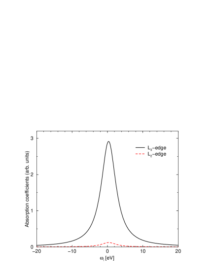
Figure 1: (Color online) Absorption coefficients $A(\omega_{i},j_{c})$ as a function of x-ray energy with $\Gamma_{c}=2.5$ eV in Case A. The (black) solid and the (red) broken lines are spectra at the Ir $L_{3}$ and $L_{2}$ edges, respectively. The origin of energy is set to be the difference between the bottom of the conduction band and the core-level energy. The absorption coefficients for the parameters in Case B are almost the same as in Case A.

IV Formula for RIXS spectra

IV.1 Second-order optical process

The RIXS spectral intensity may be expressed as the second-order optical process,

$$W(\omega_{i},q;\alpha_{i},\alpha_{f}) = 2\pi\sum_{f}\left|\sum_{n}\frac{\langle\Phi_{f}|H_{x}|\Phi_{n}\rangle\langle\Phi_{n}|H_{x}|\Phi_{i}\rangle}{\omega_{i}+\epsilon_{g}-\epsilon_{n}+i\Gamma_{c}}\right|^{2}$$ (32)

$$\times \delta(\omega_{i}+\epsilon_{g}-\omega_{f}-\epsilon_{f}).$$

The initial state is given by $|\Phi_{i}\rangle=c_{\alpha_{i}}^{\dagger}({\bf q}_{i})|0\rangle|g\rangle$, where $|g\rangle$ represents the ground state of the matter with energy $\epsilon_{g}$, and $|0\rangle$ denotes the vacuum state with photon. The intermediate state is given by $|\Phi_{n}\rangle=|0\rangle|n\rangle$, where $|n\rangle$ stands for the intermediate state of the matter with energy $\epsilon_{n}$. The final state is given by $|\Phi_{f}\rangle=c_{\alpha_{f}}^{\dagger}({\bf q}_{f})|0\rangle|f\rangle$, where $|f\rangle$ represents the final state of the matter with energy $\epsilon_{f}$. The incident photon has momentum and energy $q_{i}=({\bf q}_{i},\omega_{i})$, and polarization $\alpha_{i}$, while the scattered photon has momentum and energy $q_{f}=({\bf q}_{f},\omega_{f})$, and polarization $\alpha_{f}$. The momentum and energy transferred to the matter are accordingly given by $q=q_{i}-q_{f}=({\bf q},\omega)$.

In this second-order process, the dipole transition creates the $(5d)^{6}$-configuration at the core-hole site in the intermediate state. This state would be relaxed by hopping the excited electron to neighboring sites. Since the conduction band has the width of at most 1 eV while $\Gamma_{c}$ is as large as 2.5 eV, the energy denominator of Eq. (32) could be factored out in a reasonable accuracy. It may be hard to create additionally electron-hole pairs in the intermediate state, since the $(5d)^{6}$-configuration is almost kept at the core-hole site. Therefore, Eq. (32) may be approximated as

$$W(\omega_{i},q;\alpha_{i},\alpha_{f})$$ (33)

$$= 2\pi|R(\omega_{i},E_{0})|^{2}\sum_{f}\left|\sum_{n}\langle\Phi_{f}|H_{x}|\Phi_{n}\rangle\langle\Phi_{n}|H_{x}|\Phi_{i}\rangle\right|^{2}$$

$$\times \delta(\omega+\epsilon_{g}-\epsilon_{f}),$$

where

$$R(\omega_{i},E_{0})=\frac{1}{\omega_{i}-E_{0}+\epsilon_{\rm 2p}(j_{c})+i\Gamma_{c}}.$$ (34)

Equation (34) arises from the energy denominator factored out with $E_{0}$ being a typical energy of the conduction band. Moreover, the intensity is rewritten as

$$W(\omega_{i},q;\alpha_{i},\alpha_{f}) = |R(\omega_{i},E_{0})|^{2}\hat{M}^{\dagger}({\bf q},\alpha_{i},\alpha_{f};j_{c})$$ (35)

$$\times \hat{Y}^{+-}(q)\hat{M}({\bf q},\alpha_{i},\alpha_{f};j_{c}),$$

where

$$\left[\hat{Y}^{+-}({\bf q},\omega)\right]_{\xi_{1}\xi^{\prime}_{1};\xi\xi^{\prime}}=\int_{-\infty}^{\infty}\langle[\rho_{{\bf q}\xi_{1}\xi^{\prime}_{1}}(t)]^{\dagger}\rho_{{\bf q}\xi\xi^{\prime}}(0)\rangle{\rm e}^{i\omega t}{\rm d}t,$$ (36)

with

$$\rho_{{\bf q}\xi\xi^{\prime}}=\sqrt{\frac{2}{N}}\sum_{\bf k}d_{\xi}^{\dagger}({\bf k+q})d_{\xi^{\prime}}({\bf k}).$$ (37)

Here ${\bf k+q}$ is to be reduced back to the MBZ by a reciprocal vector ${\bf G}$, when it lies outside the MBZ. The $\hat{Y}^{+-}(q)$ represents the correlation function of the electron-hole pair excitations, which is a matrix of $144\times 144$ dimensions. The $\hat{M}({\bf q},\alpha_{i},\alpha_{f};j_{c})$ is regarded as a vector with 144 dimensions, defined by

$$\left[\hat{M}({\bf q},\alpha_{i},\alpha_{f};j_{c})\right]_{\xi\xi^{\prime}}$$ (38)

$$= \delta_{\lambda,\lambda^{\prime}}v(\lambda,{\bf q})\sum_{m}\sum_{\alpha,\beta=x,y,z}(\alpha_{i})_{\alpha}w(n\sigma;j_{c}m;\alpha)$$

$$\times w^{*}(n^{\prime}\sigma^{\prime};j_{c}m;\beta)(\alpha_{f})_{\beta},$$

with $\xi=(\lambda,n,\sigma)$ and $\xi^{\prime}=(\lambda^{\prime},n^{\prime},\sigma^{\prime})$. Since the scattering event takes place within a single site, we have the second factor from

$$v(\lambda,{\bf q}_{i})v^{*}(\lambda,{\bf q}_{f})=v(\lambda,{\bf q}_{i}-{\bf q}_{f}).$$ (39)

Note that the ${\bf q}$-dependence of $\hat{M}$ does not have the periodicity with the MBZ, leading to the RIXS intensities different between inside and outside the first MBZ.

IV.2 Correlation function within the RPA

To evaluate the correlation function, it is convenient to introduce the time-ordered Green’s function,

$$\left[\hat{Y}^{{\rm T}}(q)\right]_{\xi_{1}\xi^{\prime}_{1};\xi\xi^{\prime}}=-i\int\left\langle T\left\{[\rho_{{\bf q}\xi_{1}\xi^{\prime}_{1}}(t)]^{\dagger}\rho_{{\bf q}\xi\xi^{\prime}}(0)\right\}\right\rangle{\rm e}^{iq_{0}t}{\rm d}t.$$ (40)

The correlation function is evaluated from the Green’s function by applying the fluctuation-dissipation theorem for $\omega>0$ Igarashi and Nagao (2013b),

$$\left[\hat{Y}^{+-}(q)\right]_{\xi_{1}\xi^{\prime}_{1};\xi\xi^{\prime}}=-i\left\{\left[\hat{Y}^{{\rm T}}(q)\right]^{*}_{\xi\xi^{\prime};\xi_{1}\xi^{\prime}_{1}}-\left[\hat{Y}^{{\rm T}}(q)\right]_{\xi_{1}\xi^{\prime}_{1};\xi\xi^{\prime}}\right\}.$$ (41)

Taking account of the multiple scattering between particle-hole pair within the RPA, the Green’s function is expressed as

$$\hat{Y}^{{\rm T}}(q)=\hat{F}(q)[\hat{I}+\hat{\Gamma}\hat{F}(q)]^{-1}=\left[\hat{F}(q)^{-1}+\hat{\Gamma}\right]^{-1},$$ (42)

where

$$[\hat{\Gamma}]_{\xi_{2}\xi^{\prime}_{2};\xi_{1}\xi^{\prime}_{1}}=\Gamma^{(0)}(\xi_{2}\xi^{\prime}_{1};\xi_{1}\xi^{\prime}_{2}),$$ (43)

and the particle-hole propagator $\hat{F}(q)$ is defined as

$$[\hat{F}(q)]_{\xi_{2}\xi^{\prime}_{2};\xi_{1}\xi^{\prime}_{1}}\equiv-i\frac{2}{N}\sum_{{\bf k}}\int\frac{{\rm d}k_{0}}{2\pi}[\hat{G}({\bf k+q},k_{0}+\omega)]_{\xi_{2}\xi_{1}}[\hat{G}({\bf k},k_{0})]_{\xi^{\prime}_{1}\xi^{\prime}_{2}}.$$ (44)

By substituting Eq. (27) into the single-particle Green’s function, we get

$$[\hat{F}(q)]_{\xi_{2}\xi^{\prime}_{2};\xi_{1}\xi^{\prime}_{1}} = \frac{2}{N}\sum_{{\bf k}}\sum_{\ell,\ell^{\prime}}U_{\xi_{2}\ell}({\bf k+q})U_{\xi_{1}\ell}^{*}({\bf k+q})U_{\xi^{\prime}_{1}\ell^{\prime}}({\bf k})U_{\xi^{\prime}_{2}\ell^{\prime}}^{*}({\bf k})$$ (45)

$$\times \left[\frac{[1-n_{\ell}({\bf k+q})]n_{\ell^{\prime}}({\bf k})}{\omega-E_{\ell}({\bf k+q})+E_{\ell^{\prime}}({\bf k})+i\delta}-\frac{n_{\ell}({\bf k+q})[1-n_{\ell^{\prime}}({\bf k})]}{\omega-E_{\ell}({\bf k+q})+E_{\ell^{\prime}}({\bf k})-i\delta}\right].$$

We need a special care for the bound states, which appear below the energy continuum as a pole in $\hat{Y}^{T}(q)$. For the bound state $\omega>0$, since $\hat{F}(q)$ is a Hermite matrix, we could diagonalize $\hat{F}(q)^{-1}+\hat{\Gamma}$ by a unitary matrix. Let an eigenvalue be zero at $\omega=\omega_{B}({\bf q})$ with the eigenvector $B_{\xi\xi^{\prime}}({\bf q})$. We could expand $[\hat{Y}^{{\rm T}}(q)]_{\xi_{1}\xi^{\prime}_{1};\xi\xi^{\prime}}$ around $\omega=\omega_{B}({\bf q})$ as

$$\left[\hat{Y}^{{\rm T}}(q)\right]_{\xi_{1}\xi^{\prime}_{1};\xi\xi^{\prime}}=\frac{[\hat{C}({\bf q})]_{\xi_{1}\xi^{\prime}_{1};\xi\xi^{\prime}}}{\omega-\omega_{B}({\bf q})+i\delta},$$ (46)

where

$$[\hat{C}({\bf q})]_{\xi_{1}\xi^{\prime}_{1};\xi\xi^{\prime}}=\frac{B_{\xi_{1}\xi^{\prime}_{1}}({\bf q})B_{\xi\xi^{\prime}}^{*}({\bf q})}{\sum_{\xi_{2}\xi^{\prime}_{2}\xi_{3}\xi^{\prime}_{3}}B_{\xi_{3}\xi^{\prime}_{3}}^{*}({\bf q})\frac{\partial[\hat{F}({\bf q},\omega_{B}({\bf q}))^{-1}]_{\xi_{3}\xi^{\prime}_{3};\xi_{2}\xi^{\prime}_{2}}}{\partial\omega}B_{\xi_{2}\xi^{\prime}_{2}}({\bf q})}.$$ (47)

The correlation function is evaluated by inserting (46) into the right hand side of Eq. (41), which results in

$$\hat{Y}^{+-}(q)=2\pi\hat{C}({\bf q})\delta(\omega-\omega_{B}({\bf q})).$$ (48)

Finally, the contribution to the RIXS intensity from the bound state is given by substituting Eq. (48) into Eq. (35).

V Numerical results for RIXS spectra

We consider the specific case of a 90^∘ scattering angle in accordance with the experiments. The scattering plane is perpendicular to the IrO₂ plane, which intersects the $ab$ plane with the $[110]$ direction, as illustrated in Fig. 2. Since $\omega\sim 11.2$ keV and $|{\bf q}_{i}|\sim 5.7$ $\textrm{\AA}^{-1}$ at the Ir $L_{3}$ edge, only a few degrees of tilt of the scattering plane could sweep the entire Brillouin zone. The local coordinate frame is defined by rotating the $xy$ axes around the crystal $c$ axis with $\theta=11^{\circ}$ ($-11^{\circ}$) at A (B) sublattice, as shown in the inset of Fig. 2. Therefore the polarization vectors are represented in the local coordinate frames as

$$\alpha_{i} : \pi=\left(\frac{\cos\theta\mp\sin\theta}{2},\frac{\cos\theta\pm\sin\theta}{2},\frac{1}{\sqrt{2}}\right),$$ (49)

$$\alpha_{f} : \sigma^{\prime}=\left(\frac{\cos\theta\pm\sin\theta}{\sqrt{2}},\frac{-\cos\theta\pm\sin\theta}{\sqrt{2}},0\right),$$ (50)

$$: \pi^{\prime}=\left(-\frac{\cos\theta\mp\sin\theta}{2},-\frac{\cos\theta\pm\sin\theta}{2},\frac{1}{\sqrt{2}}\right),$$ (51)

where the upper and lower signs correspond to the A and B sublattices, respectively. The incident x ray is assumed to have the $\pi$ polarization. Inserting these relations into Eq. (38), we obtain $\hat{M}$.

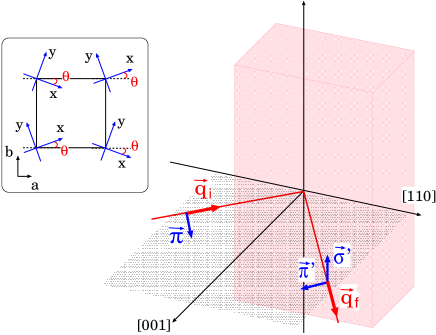
Figure 2: (Color online) Geometry of 90^∘ scattering. The scattering plane is perpendicular to the $ab$ plane and intersects the plane along the $[110]$ direction. The inset depicts the local coordinate frames, which are rotated by angle $\pm\theta$ around the $c$ axis.

V.1 Spectra for magnon

We first study the magnetic excitations emerging as bound states in $Y^{T}(q)$, which may be called as magnons. We numerically evaluate $\hat{F}(q)$ by summing over ${\bf k}$ in Eq. (45) with dividing the first MBZ into $100\times 100$ meshes. The calculation is straightforward for $\omega$ below the energy continuum. The bound states are determined by adjusting $\omega$ to give zero eigenvalue in $\hat{F}(q)^{-1}+\hat{\Gamma}$. In evaluating the corresponding intensity, we numerically carry out finite difference between $\omega=\omega_{B}({\bf q})$ and $\omega_{B}({\bf q})+0.01$eV in Eq. (47) in place of the differentiation.

Figure 3 shows the dispersion relation of magnon thus determined, and the corresponding RIXS intensities at the $L_{3}$ edge. It is found that the magnon is split into two modes with slightly different energies, as already reported Igarashi and Nagao (2014b). Although such split modes are not confirmed, their dispersion relation is in qualitative agreement with that derived from the RIXS experiment. In Case A, the energies of magnon are given by $\omega_{B}(\pi,0)=0.241$ eV and $0.252$ eV at the $X$ point, while $\omega_{B}(\pi/2,\pi/2)=0.118$ eV at the $M$ point, which slightly overestimate the magnon energies. On the other hand, in Case B, we have $\omega_{B}(\pi,0)=0.173$ eV and $0.176$ eV at the $X$ point, and $\omega_{B}(\pi/2,\pi/2)=0.149$ eV at the $M$ point, which slightly underestimate the magnon energies.

The RIXS intensity at the $L_{3}$ edge is also shown in Fig. 3. Although the energy of magnon is periodic with the MBZ, the intensity is not periodic because of the presence of $v({\bf q})$ in Eq. (38). In the narrow region around the $\Gamma$ point, the intensity of the mode with lower energy seems to diverge with $|{\bf q}|\to 0$. This arises from the staggered rotation of IrO₆ octahedra, and may be related to the presence of the weak ferromagnetism. The intensity of another mode ($\omega_{B}(0)=0.057$ eV in Case A and $0.035$ eV in Case B) is weak but finite. On the other hand, around the ${\bf q}=(\pi,\pi)$, the intensity of the mode with lower energy diverges with ${\bf q}\to(\pi,\pi)$, due to a reflection of the antiferromagnetic order. The intensity of another mode with higher energy is finite but quite large. Although the magnon peak at the $X$ point has been interpreted as being separated into a one-magnon and a weak two-magnon peaks in the RIXS experiment (Fig. 4(c) in Ref. Kim et al., 2012a), it might be more appropriate to assign the two peaks as the split modes, since the intensities of two-magnon excitations are expected to be quite small. At the $M$ point, the separation of the intensity could not be perceived, since the two modes are degenerate. It is found from the intensity curve that, across the $M$ point, the wavefunction of the mode with low energy is continuously connected to that with higher energy and vice versa. These characteristics mentioned above are consistent with the recent analysis on the basis of the localized spin model Igarashi and Nagao (2014a). For the general values of ${\bf q}$, however, the intensity varies rather strongly with changing values of ${\bf q}$, in contrast with the monotonic change found in the localized spin model.

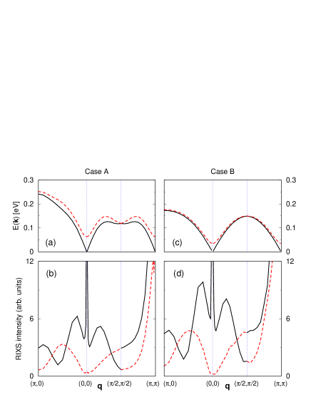
Figure 3: (Color Online) Dispersion relation of magnon and corresponding RIXS intensity for ${\bf q}$ along symmetry directions. Panels (a) and (b) are for the parameters in Case A, while panels (c) and (d) are in Case B. The (black) solid and (red) dotted lines are for the modes with lower and higher energies, respectively.

V.2 Spectra for exciton

There emerge several bound states between the magnon modes and the continuous states in the spectral function of the two-particle Green’s function. The calculation of the bound states is the same as that of the magnon modes. For $\omega$ inside the energy continuum of electron-hole pair excitations, we evaluate Eq. (45) by storing each $E_{\ell}({\bf k+q})-E_{\ell^{\prime}}({\bf k})$ into segments with the width of $0.01$ eV for $100\times 100$ ${\bf k}$-points, resulting in the histogram representation of the imaginary part of $\hat{F}(q)$. Setting $\omega$ at the center of each segment, we evaluate Eq. (45) and thereby Eq. (42), and finally Eq. (32).

Figure 4 shows the RIXS spectra thus evaluated as a function of $\omega$ for ${\bf q}$ along typical symmetry directions. The spectra are also shown without taking account of the multiple scattering ($\hat{Y}^{T}(q)$ is replaced by $\hat{F}(q)$) for reference. The $\delta$-function peaks are replaced by rectangles with their widths $0.02$ eV. It is found that the bound states bear large part of exciton intensities. The exciton peaks are close to the magnon peaks around the $X$ and $M$ points in Case A, while they are well separated from the magnon peaks in Case B in agreement with the RIXS experiment. Since the bound states of excitons are composed mainly of the $j_{\rm eff}=1/2$ states of electron and $j_{\rm eff}=3/2$ states of hole, the larger value of $\zeta_{\rm SO}$ in Case B may lead to the larger separation between the exciton and magnon peaks. In the localized electron picture, the exciton peak is given by the excitation from the $j_{\rm eff}=3/2$ manifold to the $j_{\rm eff}=1/2$ manifold, where the dispersion is given by the hopping in the antiferromagnetic isospin background Kim et al. (2012b); Ament et al. (2011b).

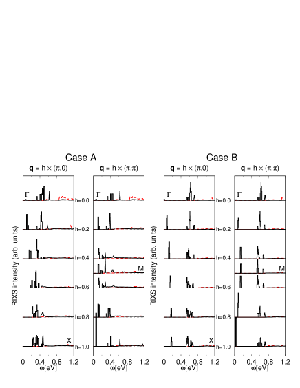
Figure 4: (Color Online) The RIXS spectra as a function of energy loss $\omega$ for ${\bf q}$ along symmetry directions. The (black) solid and (red) broken lines correspond to the intensities with and without taking account of the multiple scattering, respectively. The $\delta$-function peaks are replaced by rectangles with their widths $0.02$ eV.

For comparison with the experimental RIXS spectra, the calculated spectra are convoluted with the Lorentzian function with the full width half maximum $0.04$ eV. Figure 5 shows the result in Case B. The peak with the lowest energy represents the magnon contribution. The intensity diverging at $\omega=0$ is excluded at the $\Gamma$ point. The split of magnon modes could not be distinguished at the $X$ point due to the convolution. The intensities of exciton peaks are two or three times larger than those of magnon modes, which ratio is comparable with the experiment Kim et al. (2012a).

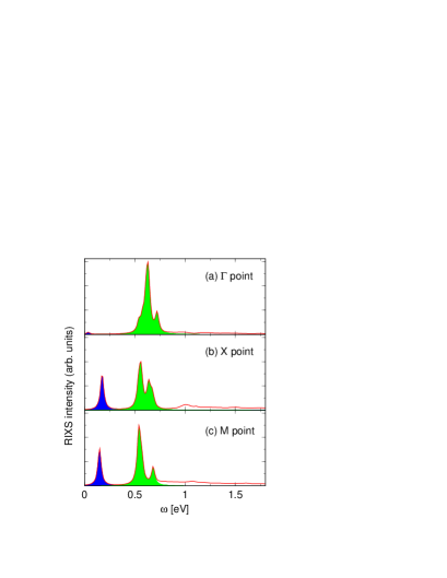
Figure 5: (Color Online) The RIXS spectra for both the magnon and exciton excitations as a function of energy loss $\omega$ at (a) the $\Gamma$, (b) $X$, and (c) $M$ points, with $\zeta_{\rm SO}=0.45$ eV and $t_{2}=0.25$ eV (Case B). The spectra are convoluted with Lorentzian function with the full width half maximum 0.04 eV. The (blue) filled area around the peak with the lowest energy represents the magnon contribution. The contribution from the bound state of exciton is represented by the (green) filled area around $\omega\simeq 0.5-0.7$ eV. The divergent intensity at $\omega=0$ are excluded at the $\Gamma$ point.

VI Concluding remarks

We have analyzed the $L$-edge RIXS spectra from Sr₂IrO₄ in an itinerant electron approach. Introducing a multi-orbital tight-binding model, we have calculated the one-electron energy band within the HFA, and the Green’s functions for particle-hole pair excitations within the RPA. The RIXS spectra have been evaluated from the Green’s functions within the FCA. We have found two kinds of peaks in the RIXS spectra.

One is the peak of magnon, which arises from the bound state in $\hat{Y}^{T}(q)$. The dispersion of magnon is obtained in agreement with the experiment Kim et al. (2012a). We have predicted two-peak structures with slightly different excitation energy $\sim 0.05$ eV due to the split of magnon modes. Since the instrumental resolution is the same order of the split, it seems hard to detect the split in RIXS experiments. Some clue of the split, however, might be found with a careful examination of the spectral shape or by improving the experimental energy resolution.

Another is the peak of exciton, which also arises from the bound states in $\hat{Y}^{T}(q)$. We have found large intensities concentrated on these peaks in comparison with the intensities of continuous states. The peak positions relative to the magnon peaks depend on parameters. The larger value of $\zeta_{\rm SO}$ and the smaller value of $t_{2}$ (Case B) seem to give the exciton peaks in better position in comparison with the RIXS experiment. To make quantitative understanding of the spectra, however, it may be necessary to refine the present model by including the hopping electron to further neighbors as well as the tetragonal crystal field or by including more correlation effects beyond the HFA and RPA. Studies along this direction are left in future.