Spectroscopic parameters for solar-type stars with moderate/high rotation.

Abstract

Context. Planetary studies demand precise and accurate stellar parameters as input to infer the planetary properties. Different methods often provide different results that could lead to biases in the planetary parameters.

Aims. In this work, we present a refinement of the spectral synthesis technique designed to treat better more rapidly rotating FGK stars. This method is used to derive precise stellar parameters, namely effective temperature, surface gravity, metallicitity and rotational velocity. This procedure is tested for samples of low and moderate/fast rotating FGK stars.

Methods. The spectroscopic analysis is based on the spectral synthesis package Spectroscopy Made Easy (SME), assuming Kurucz model atmospheres in LTE. The line list where the synthesis is conducted, is comprised of iron lines and the atomic data are derived after solar calibration.

Results. The comparison of our stellar parameters shows good agreement with literature values, both for low and for higher rotating stars. In addition, our results are on the same scale with the parameters derived from the iron ionization and excitation method presented in our previous works. We present new atmospheric parameters for 10 transiting planet-hosts as an update to the SWEET-Cat catalogue. We also re-analyze their transit light curves to derive new updated planetary properties.

1 Introduction

Since the first discoveries of the extrasolar planets, it became clear that the derivation of their fundamental properties was directly linked to the properties of their host stars. Until recently the discovery of extrasolar planets was substantially fed by the radial velocity (RV) technique. In the last years, several space missions such as CoRoT (Baglin et al. 2006) and Kepler (Borucki et al. 2010), as well as ground based surveys like WASP (Pollacco et al. 2006)) and HAT-P (Bakos et al. 2004) are successfully using the transit technique. The large number of planets discovered today, allows the study of correlations in the properties of planets and their parent stars, providing strong observational constrains on the theories of planet formation and evolution (Mordasini et al. 2012, and references therein).

To understand the physical processes involved in the formation and evolution of planetary systems, precise measurements of the fundamental properties of the exoplanets and their hosts are required. From the analysis of the light curve of a transiting planet, the planetary radius determination is always dependent on the stellar radius (R_p $\propto$ R_⋆). Moreover, the mass of the planet, or the minimum mass in case the inclination of the orbit is not known, is calculated from the RV curve only if the mass of the star is known (M_p $\propto$ M${}_{\star}^{2/3}$). The fundamental stellar parameters of mass and radius, on the other hand, depend on observationally determined parameters such as effective temperature ($T_{\mathrm{eff}}$), surface gravity ($\log g$), and metallicitity ($[Fe/H]$, where iron is usually used as a proxy). The latter fundamental parameters are used to deduce stellar mass and radius either from calibrations (Torres et al. 2010; Santos et al. 2013) or stellar evolution models (e.g. Girardi et al. 2002).

It is therefore, imperative to derive precise and accurate stellar parameters to avoid the propagation of errors in the planetary properties. For instance, Torres et al. (2012) have shown that unconstrained parameter determinations derived from spectral synthesis techniques introduce considerable systematic errors in the planetary mass and radius. In particular, residual biases of the stellar radius may explain part of the anomalously inflated radii that has been observed for some Jovian planets such as in the cases of HD 209458 b (Burrows et al. 2000) and WASP-12 b (Hebb et al. 2009).

There are several teams applying different analysis techniques (e.g. photometric, spectroscopic, interferometric), atomic data, model atmospheres, etc., and their results often yield significant differences (e.g. Torres et al. 2008; Bruntt et al. 2012; Molenda-Żakowicz et al. 2013). These systematic errors are difficult to assess and are usually the main error contributors within a study. Such problems can be mitigated by a uniform analysis that will yield the precision needed. Apart from minimizing the errors of the stellar/planet parameters, uniformity can enhance the statistical significance of correlations between the presence of planets and the properties of their hosts. For example, an overestimation in the stellar radius has been reported in some samples of Kepler Objects of Interest (Verner et al. 2011; Everett et al. 2013) which in turn leads to overestimated planetary radius. In this case, planets are perhaps misclassified in the size range likely for rocky Earth-like bodies, affecting the planet occurrence rate of Earth-sized planets around solar-type stars.

The high quality stellar spectra obtained from RV planet search programs (e.g. Sousa et al. 2008, 2011), make spectroscopy a powerful tool for deriving the fundamental parameters in absence of more direct radius measurements (restricted only to limited stars with the interferometric technique or stars that belong to eclipsing binaries). A typical method of deriving stellar parameters for solar-type stars is based on the excitation and ionization equilibrium by measuring the equivalent widths (EW) of iron lines (hereafter EW method). This method has successfully been applied to RV targets that are restricted to low rotational velocities ($\upsilon\sin i$) to increase the precision of the RV technique (Bouchy et al. 2001). High rotational velocities also limit the precision of the EW method. Spectral lines are broadened by rotation and therefore neighboring lines become blended, often unable to resolve. Even though the EW is preserved, its correct measurement is not yet possible.

On the other hand, the transit planet-hosts have a wider dispersion in rotation rates when comparing to the slow rotating FGK hosts observed with the RV technique. For moderate/high rotating stars, which may be the case of the transit targets, spectral synthesis is required for the parameter determination. This technique yields stellar parameters by fitting the observed spectrum with a synthetic one (e.g. Valenti & Fischer 2005; Malavolta et al. 2014) or with a library of pre-computed synthetic spectra (e.g. Recio-Blanco et al. 2006).

In this paper, we propose a refined approach based on the spectral synthesis technique to derive stellar parameters for low-rotating stars (Sect. 2), yielding results on the same scale with the homogeneous analysis of our previous works (Sect. 3). Our method is tested for a sample of moderate/high FGK rotators (Sect. 4) and also is applied to a number of planet-hosts providing new stellar parameters. Their planetary properties are also revised (Sect. 5).

2 Spectroscopic analysis

Due to severe blending, measuring the EW of stars with high rotational velocity is very difficult, if not impossible (e.g. see Fig. 1). In this paper, we are focusing on deriving precise and accurate parameters for stars with higher $\upsilon\sin i$ using the spectral synthesis technique.

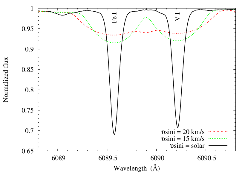
Figure 1: Solar absorption lines (solid line), broadened by $\upsilon\sin i$ 15 km/s (green) and 20 km/s (red). Blending at these rates due to rotation makes the accurate measurement of the EW very difficult.

2.1 Line list

For an accurate spectral synthesis, atomic and molecular data of all lines in the wavelength intervals where the synthesis is conducted must be as accurate as possible. The choice of intervals for our analysis is based on the line list of iron lines as described in Tsantaki et al. (2013). This list is comprised of weak, isolated iron lines, specifically chosen from the extended line list of Sousa et al. (2008) to exclude blended lines that are commonly found in K-type stars. Effective temperatures derived with this line list are in agreement with the InfraRed-Flux Method (IRFM) for the whole temperature regime of FGK dwarfs.

The spectral window around each iron line is set wide enough to include broadened lines of $\upsilon\sin i$ $\sim$ 50 km/s. Following the Doppler law, such a rotational velocity causes a broadening of $\pm$ 1 Å, around a line in the middle of the optical wavelength range ($\sim$ 5500 Å).

The original line list contains 137 ${Fe\textsc{i}}$ and ${Fe\textsc{ii}}$ lines where we set intervals of 2 Å around them. The atomic data for these intervals were obtained from the Vienna Atomic Line Database (Piskunov et al. 1995; Kupka et al. 1999). We extracted atomic data for all the expected transitions for a star with solar atmospheric parameters for our wavelength intervals. We also included lines predicted for a K-type star with $T_{\mathrm{eff}}$ = 4400 K. The two line lists that correspond to atomic transitions for the two different spectral types were merged into one after removing duplicates. Molecular data of the most abundant molecules in solar-type stars (C₂, CN, OH, and MgH) were also obtained from VALD using the same requests as for the atomic data.

From the above intervals we selected the optimal ones according to the following procedure. From the first analyses, we noticed that K-type stars show the highest residuals between the observed and the best-fit synthetic spectrum compared to the F and G spectral types. The main reason is that the spectra of K-type stars include numerous lines but not all appear in our line list after the requested atomic data queries. Therefore, we discarded lines in the bluer part (below 5000 Å) where lines are more crowded. Lines within overlapping intervals were merged into one.

In addition, we checked the behaviour of the remaining lines due to rotation by using the Sun as a reference star convolved with moderate rotation of 20 km/s (see Sect. 4). We excluded lines by eye where there was strong contamination by neighboring lines due to broadening and chopped the intervals were the contamination in the edges was weak. We also excluded lines that showed high residuals between the spectrum and the synthesized one for the solar parameters.

The initial choice of spectral windows was double the length i.e. 4 Å where the iron lines were placed in the center. For these intervals even though the best-fit parameters for the Sun (low rotation) were accurate, for the solar spectrum convolved with rotation (again of 20 km/s), the parameters showed higher deviation ($T_{\mathrm{eff}}$ = 5728 K, $\log g$ = 4.39 dex, [Fe/H] = -0.03 dex) compared to the standard solar values. For this reason we limited the length of the intervals to 2 Å.

Except for blending, another considerable problem that limits this procedure because of high rotation is the difficulty in distinguishing between the line and the continuum points as the lines become very shallow. In this case, the wings of the lines are miscalculated as continuum, leading to the biases in Sect 4.

Taking all the above into consideration, the final line list is comprised of 47 Fe i and 4 Fe ii lines into 42 wavelength intervals, summing in total of 537 lines of different species. The wavelength intervals and the atomic data of the iron lines are presented at Table 1.

Table 1: Spectral wavelength intervals and line data used for the spectroscopic analysis.

Intervals	$\lambda$	Species	$\chi_{ex}$	$\log gf$	$\varGamma_{6}$
Å	Å		(eV)
5521.45 - 5523.45	5522.45	Fe i	4.21	-1.484	-7.167
5559.22 - 5561.11	5560.22	Fe i	4.43	-0.937	-7.507
5632.95 - 5634.95	5633.95	Fe i	4.99	-0.186	-7.391
5648.99 - 5652.47	5649.99	Fe i	5.10	-0.649	-7.302
…	5651.47	Fe i	4.47	-1.641	-7.225
…	5652.32	Fe i	4.26	-1.645	-7.159
5678.03 - 5680.97	5679.03	Fe i	4.65	-0.657	-7.320
…	5680.24	Fe i	4.19	-2.347	-7.335
5719.90 - 5721.90	5720.90	Fe i	4.55	-1.743	-7.136
5792.92 - 5794.92	5793.92	Fe i	4.22	-2.038	-7.304
5810.92 - 5812.92	5811.92	Fe i	4.14	-2.323	-7.951
5813.81 - 5815.45	5814.81	Fe i	4.28	-1.720	-7.269
…	5815.22	Fe i	4.15	-2.521	-7.038
5852.15 - 5854.15	5852.22	Fe i	4.55	-1.097	-7.201
…	5853.15	Fe i	1.49	-5.006	-6.914
5861.36 - 5863.36	5862.36	Fe i	4.55	-0.186	-7.572
5986.07 - 5988.07	5987.07	Fe i	4.79	-0.428	-7.353
6004.55 - 6006.55	6005.55	Fe i	2.59	-3.437	-7.352
6088.57 - 6090.57	6089.57	Fe i	4.58	-1.165	-7.527
6119.25 - 6121.25	6120.25	Fe i	0.92	-5.826	-7.422
6126.91 - 6128.78	6127.91	Fe i	4.14	-1.284	-7.687
6148.25 - 6150.25	6149.25	Fe ii	3.89	-2.786	-7.478
6150.62 - 6152.62	6151.62	Fe i	2.18	-3.188	-7.729
6156.73 - 6158.73	6157.73	Fe i	4.08	-1.097	-7.691
6172.65 - 6174.19	6173.34	Fe i	2.22	-2.775	-7.829
6225.74 - 6227.40	6226.74	Fe i	3.88	-2.021	-7.423
6231.65 - 6233.65	6232.65	Fe i	3.65	-1.161	-7.552
6237.00 - 6239.38	6238.39	Fe ii	3.89	-2.693	-7.359
6321.69 - 6323.69	6322.69	Fe i	2.59	-2.314	-7.635
6334.34 - 6336.34	6335.34	Fe i	2.20	-2.323	-7.735
6357.68 - 6359.68	6358.68	Fe i	0.86	-4.225	-7.390
6431.83 - 6433.05	6432.69	Fe ii	2.89	-3.650	-7.391
6455.39 - 6457.02	6456.39	Fe ii	3.90	-2.175	-7.682
6480.88 - 6482.88	6481.88	Fe i	2.28	-2.866	-7.627
6626.55 - 6628.55	6627.55	Fe i	4.55	-1.400	-7.272
6645.94 - 6647.50	6646.94	Fe i	2.61	-3.831	-7.141
6698.15 - 6700.15	6699.15	Fe i	4.59	-2.004	-7.162
6704.11 - 6706.11	6705.11	Fe i	4.61	-1.088	7.539
6709.32 - 6711.32	6710.32	Fe i	1.49	-4.732	-7.335
6724.36 - 6727.67	6725.36	Fe i	4.10	-2.093	-7.302
…	6726.67	Fe i	4.61	-0.951	-7.496
6731.07 - 6732.50	6732.07	Fe i	4.58	-2.069	-7.130
6738.52 - 6740.52	6739.52	Fe i	1.56	-4.797	-7.685
6744.97 - 6746.97	6745.11	Fe i	4.58	-2.047	-7.328
…	6745.97	Fe i	4.08	-2.603	-7.422
6839.23 - 6840.84	6839.84	Fe i	2.56	-3.304	-7.567
6854.72 - 6856.72	6855.72	Fe i	4.61	-1.885	-7.253
6856.25 - 6859.15	6857.25	Fe i	4.08	-1.996	-7.422
…	6858.15	Fe i	4.61	-0.941	-7.344
6860.94 - 6862.94	6861.94	Fe i	2.42	-3.712	-7.580
…	6862.50	Fe i	4.56	-1.340	-7.330

Atomic data are usually calculated from laboratory or semi-empirical estimates. In order to avoid uncertainties that may arise from such estimations, we determine astrophysical values for the basic atomic and molecular line data namely for the oscillator strengths ($\log gf$) and the van der Waals damping parameters ($\varGamma_{6}$). We used the National Solar Observatory Atlas (Kurucz et al. 1984) to improve the transition probabilities and the broadening parameters of our line list in an inverted analysis using the typical solar parameters fixed (as adopted by Valenti & Fischer (2005): $T_{\mathrm{eff}}$ = 5770 K, $\log g$ = 4.44 dex, $[Fe/H]$ = 0.0 dex, $\upsilon_{mic}$ = 0.87 km/s, $\upsilon_{mac}$ = 3.57 km/s, $\log_{\epsilon}(Fe)$ = 7.50 dex).

2.2 Initial conditions

All minimization algorithms depend on the initial conditions. In order to make sure that the convergence is achieved for the global minimum, we set the initial conditions as close to the expected ones as possible. For temperature, we use the calibration of Valenti & Fischer (2005) as a function of B –V color. Surface gravities are calculated using Hipparcos parallaxes (van Leeuwen 2007), V magnitudes, bolometric corrections based on Flower (1996) and Torres (2010), and solar magnitudes from (Bessell et al. 1998). In cases the parallaxes are not available, we use the literature values. Masses are set to solar value.

Microturbulence ($\upsilon_{mic}$) is used to remove possible trends in parameters due to model deficiencies. It has been shown that $\upsilon_{mic}$ correlates mainly with $T_{\mathrm{eff}}$ and $\log g$ for FGK stars (e.g. Nissen 1981; Adibekyan et al. 2012a; Ramírez et al. 2013). We therefore, set $\upsilon_{mic}$ according to the correlation discussed in the work of Tsantaki et al. (2013) for a sample of FGK dwarfs. For the giant stars in our sample, we use the empirical calibration of Mortier et al. (2013a) based on the results of Hekker & Meléndez (2007).

Macroturbulence ($\upsilon_{mac}$) is a broadening mechanism that also correlates with $T_{\mathrm{eff}}$ (e.g. Saar & Osten 1997). We set $\upsilon_{mac}$ in our analysis following the relation of Valenti & Fischer (2005). Initial metallicity ($[M/H]$) is set to solar and initial rotational velocity to 0.5 km/s.

2.3 Spectral synthesis

The spectral synthesis package we use for this analysis is Spectroscopy Made Easy (SME), version 3.3 (Valenti & Piskunov 1996). Modifications from the first version are described in Valenti et al. (1998) and Valenti & Fischer (2005). The adopted model atmospheres are generated by the ATLAS9 program (Kurucz 1993) and local thermodynamic equilibrium is assumed. SME includes the parameter optimization procedure based on the Levenberg-Marquardt algorithm to solve the nonlinear least-squares problem yielding the parameters that minimize the $\chi^{2}$. In our case, the free parameters are: $T_{\mathrm{eff}}$, $\log g$, $[M/H]$, and $\upsilon\sin i$. Metallicity in this work refers to the average abundance of all elements producing absorption in our spectral regions. We can safely assume that $[M/H]$ approximately equals to $[Fe/H]$ for our sample of stars as the dominant lines in our regions are the iron ones. Additionally, these stars are not very metal-poor ($>$ -0.58 dex). The overall metallicity in metal-poor stars is enhanced by other elements (relative to iron) and in that case the previous assumption does not hold (e.g. Adibekyan et al. 2012b).

After a first iteration with the initial conditions described above, we use the output set of parameters to derive stellar masses using the Padova models (da Silva et al. 2006). Surface gravity is then re-derived with the obtained mass and temperature. The values of $\upsilon_{mic}$ and $\upsilon_{mac}$ are also updated by the new $T_{\mathrm{eff}}$ and $\log g$. The final results are obtained after a second iteration with the new initial values. Additional iterations were not required, as the results between the first and second iteration in all cases were very close (for instance the mean differences for the sample in Sect.4 are: $\Delta T_{\mathrm{eff}}$ = 24 K, $\Delta\log g$ = 0.06 dex, $\Delta$[Fe/H] = 0.003 dex and $\Delta\upsilon\sin i$ = 0.18 km/s).

2.4 Internal error analysis

Estimation of the errors is a complex problem for this analysis. One approach is to calculate the errors from the covariance matrix of the best fit solution. Usually these errors are underestimated and do not include deviations depending on the specific choice of initial parameters nor the choice of the wavelength intervals. On the other hand, Monte Carlo approximations are computational expensive when we are dealing with more than a handful of stars. In this section we explore the contribution of different type of errors for reference stars of different spectral types. The errors of these stars will be representative of the errors of the whole group that each one belongs.

We select 3 slow rotating stars of different spectral types: F (HD 61421), G (Sun), and K (HD 20868) as our references. Their stellar parameters are listed in Table 9. We convolve each of these stars with different rotational profiles (initial, 15, 25, 35, 45, and 55 km/s) to quantitatively check the errors attributed to different $\upsilon\sin i$ (see also Sect 4).

Our aim is to calculate the errors from two different sources: 1) the initial conditions, and 2) the choice of wavelength intervals. Firstly, we check how the initial parameters affect the convergence to the correct ones. For each star we set different initial parameters by changing: $T_{\mathrm{eff}}$ $\pm$ 100 K, $\log g$ $\pm$ 0.20 dex, $[Fe/H]$ $\pm$ 0.10 dex, and $\upsilon\sin i$ $\pm$ 0.50 km/s. We calculate the parameters for the total 81 permutations of the above set of initial parameters. This approach is also presented in Valenti & Fischer (2005) for their solar analysis.

The choice of wavelength intervals is also important for the precise determination of stellar parameters. The spectral window of different instruments varies and therefore not all wavelength intervals of a specific line list can be used for the parameter determination. Moreover, there are often other reasons for which discarding a wavelength interval would be wise, such as the presence of cosmic rays. In these cases, the errors which are attributed to the discarded wavelength intervals from a defined line list can give an estimation on the homogeneity of our parameters.

We account for such errors by randomly excluding 10% of our total number of intervals (that leaves us with 38 intervals). This percentage is approximately expected for the above cases. Stellar parameters are calculated for the shortened list of intervals and this procedure is repeated 100 times (each time discarding a random 10%). The error of each free parameter is defined as the standard deviation of the results of all repetitions.

For our analysis, we do not include the errors derived from the convariance matrix. The primary reason is that the flux errors of each wavelength element that are required for the precise calculation of the convariance matrix, unfortunately, are not provided for our spectra. Therefore, in such cases one has to be careful with the interpretation of the values of the covariance matrix.

Table 2 shows the errors derived from the two different sources described above. The errors in $T_{\mathrm{eff}}$ and $\log g$ due to the different initial parameters are slightly more significant whereas for $[Fe/H]$ and $\upsilon\sin i$ both type of errors are comparable. Finally, we add quadratically the 2 sources of errors that are described above (see Table 3). We notice that for higher $\upsilon\sin i$, the uncertainties in all parameters become higher as one would expect. K-type stars have also higher uncertainties compared to F- and G-types. In particular, the uncertainties in $\upsilon\sin i$, for K-type stars, are significantly high for $\upsilon\sin i>$ 45 km/s. Fortunately, K-type stars are typically low rotators since rotational velocity decreases with the spectral type for FGK stars (e.g. Gray 1984; Nielsen et al. 2013).

Table 2: Internal error analysis for each spectral type and different rotational velocities. Two sources of errors were considered: Initial parameters and Wavelength choice (dependence on the choice of the 90% of the total intervals). Rotational velocity 0 km/s refers to the intrinsic $\upsilon\sin i$ of the star.

Parameters	F-type (HD 61421)
	Initial parameters						Wavelength choice
$\upsilon\sin i$	0 km/s	15 km/s	25 km/s	35 km/s	45 km/s	55 km/s	0 km/s	15 km/s	25 km/s	35 km/s	45 km/s	55 km/s
$T_{\mathrm{eff}}$ (K)	27	43	48	54	97	108	13	9	17	48	16	85
$\log g$ (dex)	0.11	0.15	0.21	0.25	0.20	0.17	0.02	0.02	0.08	0.16	0.03	0.05
$[Fe/H]$ (dex)	0.03	0.04	0.05	0.07	0.06	0.07	0.01	0.01	0.02	0.04	0.01	0.01
$\upsilon\sin i$ (km/s)	0.20	0.25	0.98	1.00	1.57	2.60	0.08	0.14	0.91	0.89	0.93	2.13
	G-type (Sun)
	Initial parameters						Wavelength choice
$\upsilon\sin i$	0 km/s	15 km/s	25 km/s	35 km/s	45 km/s	55 km/s	0 km/s	15 km/s	25 km/s	35 km/s	45 km/s	55 km/s
$T_{\mathrm{eff}}$ (K)	12	5	18	86	86	147	13	9	21	36	43	116
$\log g$ (dex)	0.06	0.05	0.09	0.16	0.11	0.14	0.01	0.03	0.07	0.07	0.07	0.12
$[Fe/H]$ (dex)	0.02	0.01	0.04	0.07	0.07	0.07	0.02	0.01	0.03	0.02	0.02	0.04
$\upsilon\sin i$ (km/s)	0.25	0.09	0.32	0.36	2.47	3.67	0.11	0.99	0.26	0.17	2.29	3.49
	K-type (HD 20868)
	Initial parameters						Wavelength choice
$\upsilon\sin i$	0 km/s	15 km/s	25 km/s	35 km/s	45 km/s	55 km/s	0 km/s	15 km/s	25 km/s	35 km/s	45 km/s	55 km/s
$T_{\mathrm{eff}}$ (K)	20	52	54	77	130	127	15	47	45	68	110	110
$\log g$ (dex)	0.09	0.16	0.17	0.20	0.14	0.18	0.03	0.11	0.12	0.16	0.10	0.09
$[Fe/H]$ (dex)	0.02	0.06	0.09	0.09	0.09	0.09	0.02	0.05	0.07	0.07	0.02	0.01
$\upsilon\sin i$ (km/s)	0.46	0.72	0.86	2.38	6.92	7.54	0.45	0.69	0.77	2.12	6.98	7.36

Table 3: Errors summed quadratically for each spectral type and for the different rotational velocities.

Parameters	F-type (HD 61421)
$\upsilon\sin i$	0 km/s	15 km/s	25 km/s	35 km/s	45 km/s	55 km/s
$T_{\mathrm{eff}}$ (K)	30	44	51	72	98	137
$\log g$ (dex)	0.11	0.15	0.22	0.30	0.20	0.18
$[Fe/H]$ (dex)	0.03	0.04	0.05	0.03	0.08	0.06
$\upsilon\sin i$ (km/s)	0.22	0.29	1.34	1.34	1.82	3.36
	G-type (Sun)
$\upsilon\sin i$	0 km/s	15 km/s	25 km/s	35 km/s	45 km/s	55 km/s
$T_{\mathrm{eff}}$ (K)	18	10	28	93	96	187
$\log g$ (dex)	0.06	0.06	0.11	0.17	0.13	0.18
$[Fe/H]$ (dex)	0.03	0.01	0.05	0.07	0.07	0.08
$\upsilon\sin i$ (km/s)	0.27	0.99	0.41	0.40	3.37	5.06
	K-type (HD 20868)
$\upsilon\sin i$	0 km/s	15 km/s	25 km/s	35 km/s	45 km/s	55 km/s
$T_{\mathrm{eff}}$ (K)	25	70	70	103	170	168
$\log g$ (dex)	0.09	0.19	0.21	0.26	0.17	0.20
$[Fe/H]$ (dex)	0.03	0.08	0.11	0.11	0.09	0.09
$\upsilon\sin i$ (km/s)	0.64	0.99	1.15	3.19	9.83	10.54

3 Spectroscopic parameters for low rotating FGK stars

To test the effectiveness of the line list, we use a sample of 48 FGK stars (40 dwarfs and 8 giants) with slow rotation, high S/N and high resolution spectra, most of them taken from the archival data of HARPS (R $\sim$ 110000) and the rest with UVES (R $\sim$ 110000) and FEROS (R $\sim$ 48000) spectrographs. Their stellar parameters range from: 4758 $\leq T_{\mathrm{eff}}\leq$ 6666 K, 2.82 $\leq\log g\leq$ 4.58 dex, and -0.58 $\leq$ [Fe/H] $\leq$ 0.33 dex and are derived following the method described in Sect. 2. Figure 2 depicts the comparison between the parameters derived in this work and the EW method. All parameters from the EW method were taken from Sousa et al. (2011); Mortier et al. (2013a, b); Tsantaki et al. (2013); Santos et al. (2013) using the same methodology that provides best possible homogeneity for the comparison. The differences between these methods are presented in Table 4 and the stellar parameters in Table 9.

Table 4: Differences in stellar parameters between this work and the EW method for the 48 sample stars. MAD values correspond to the median average deviation and are indicated in parenthesis. The differences are also listed per spectral type. N is the number of stars used for the comparison.

This Work – EW	$\Delta T_{\mathrm{eff}}$ ($\pm$ MAD) K	$\Delta\log g$ ($\pm$ MAD) dex	$\Delta$ [Fe/H] ($\pm$ MAD) dex	N
Whole sample	-26 $\pm$ 14 ($\pm$ 55)	-0.19 $\pm$ 0.04 ($\pm$ 0.14)	0.000 $\pm$ 0.010 ($\pm$ 0.041)	48
F-type	-97 $\pm$ 22 ($\pm$ 68)	-0.34 $\pm$ 0.07 ($\pm$ 0.18)	0.006 $\pm$ 0.014 ($\pm$ 0.014)	12
G-type	7 $\pm$ 16 ($\pm$ 36)	-0.07 $\pm$ 0.05 ($\pm$ 0.04)	0.019 $\pm$ 0.021 ($\pm$ 0.032)	18
K-type	-5 $\pm$ 27 ($\pm$ 32)	-0.18 $\pm$ 0.05 ($\pm$ 0.16)	-0.027 $\pm$ 0.016 ($\pm$ 0.042)	18

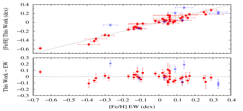
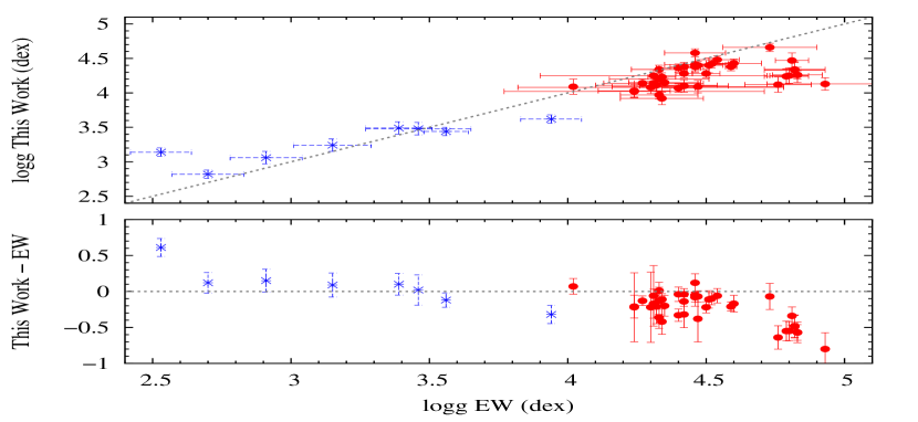
Figure 2: Comparison between the parameters derived using the spectral synthesis method (This Work) and the results of our EW method: temperature (top panel), metallicitity (middle panel) and surface gravity (bottom panel). Circles represent dwarf stars and asterisks giants.

The effective temperatures derived with the spectral synthesis technique and the EW method are in good agreement. The greatest discrepancies appear for $T_{\mathrm{eff}}>$ 6000 K, where the effective temperature derived from this work is systematically cooler. The same systematics are also presented in Molenda-Żakowicz et al. (2013), where the authors compare the EW method with other spectral synthesis techniques but the explanation for these discrepancies is not yet clear.

The values of metallicitity are in perfect agreement between the two methods.

Surface gravity is a parameter that is the most difficult to constrain with spectroscopy. The comparison of the two methods shows a considerable offset of 0.19 dex, where $\log g$ is underestimated compared to the EW method. Interestingly, this offset is smaller for giant stars ($\Delta\log g$ = 0.07 dex) than for dwarfs ($\Delta\log g$ = -0.24 dex).

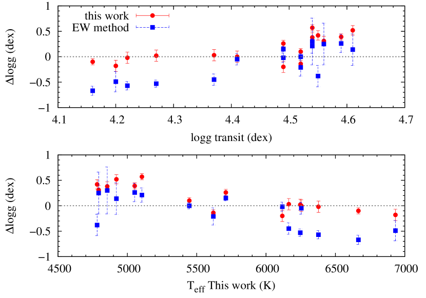
Figure 3: Comparison of surface gravity derived from the transit fit with this work and the EW method. $\Delta\log g$ represents ’transit minus this work’ (red circles) and ’transit minus EW method’ (blue squares).

To further investigate these differences, we compare the spectroscopic $\log g$ with surface gravity derived with another method that is less model dependent. For 16 dwarf stars in our sample that have a transiting planet, surface gravity can be derived from the analysis of the transit light curve (see also Sect. 5). We compare $\log g$ derived from the transit light curve with the spectroscopic $\log g$ from the EW method (both values are taken from Mortier et al. (2013b)) and this work (see Fig. 3).

We show that $\log g$ from the EW analysis is overestimated for low $\log g$ values and underestimated for high $\log g$ values. Fortunately, this trend does not affect $T_{\mathrm{eff}}$ and $[Fe/H]$ as shown in the recent work of Torres et al. (2012). Same systematics were also found between the $\log g$ from the EW method and the $\log g$ derived with the Hipparcos parallaxes for solar-type stars in Tsantaki et al. (2013) and Bensby et al. (2014). These results imply that $\log g$ from the EW method using iron lines suffers from biases, but there is no clear explanation for the reasons.

On the other hand, $\log g$ derived from this work is in very good agreement with the transit $\log g$, for values lower than 4.5 dex. Stars with $\log g>$ 4.5 dex correspond to the cooler stars and are also underestimated. The reason for this underestimation is not yet known and further investigation is required to understand this behaviour.

Despite the differences for the $\log g$ values of mainly the F-type stars, the results listed in Table 4 show that for low rotating FGK stars, stellar parameters derived from both methods are on the same scale. This means that for the whole sample the residuals between both methods are small and of the same order of magnitude as are the errors of the parameters.

4 Spectroscopic parameters for high rotating FGK dwarfs

Testing our method for low FGK rotators does not necessary imply that it will work for higher $\upsilon\sin i$ where spectral lines are much broadened and shallower. Our goal is to examine how efficient our method is for moderate/high rotating stars. For this purpose, we derive stellar parameters for reference stars of different spectral type and with low $\upsilon\sin i$. Secondly, these stars are convolved with a set of rotational profiles using the rotin3 routine as part of the SYNSPEC synthesis code (Hubeny et al. 1994). As a result, each star has 8 different rotational velocities (initial, 5, 10, 15, 20, 25, 30, 40, 50 km/s). Stellar parameters of all rotational profiles are calculated to investigate how they differ from the non-broadened (unconvolved) star. This test is an indication of how the accuracy of our method is affected by adding a rotational profile.

The selected reference stars are: two F-type, one G-type, and four K-type stars and are presented in boldface in Table 9. Probably one star per spectral type would be enough but we included more F- and K-type stars because they showed higher uncertainties (especially the K-type stars). In Fig. 4 the differences of stellar parameters between the stars with the unconvolved values (original $\upsilon\sin i$) and the convolved ones are plotted for the 8 different rotational velocities.

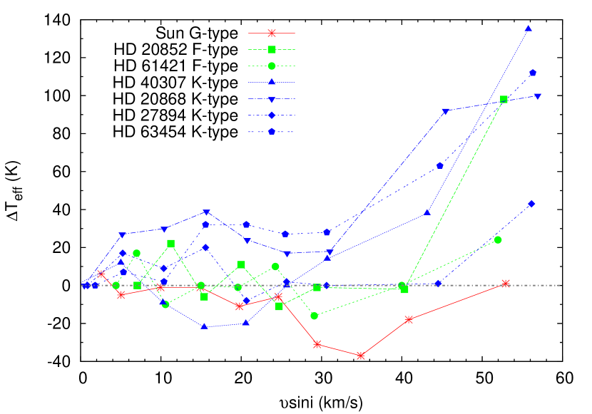
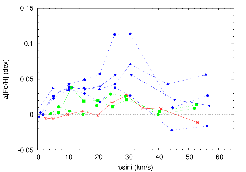
Figure 4: Differences in temperature (top panel), surface gravity (middle panel) and metallicitity (bottom panel) (initial $\upsilon\sin i$ minus the different rotational profiles) vs. $\upsilon\sin i$. Each star is represented with different symbol and each spectral type is represented with different colour. Blue for K-type, red for G-type and green F-type. The initial $\upsilon\sin i$ is different for each star.

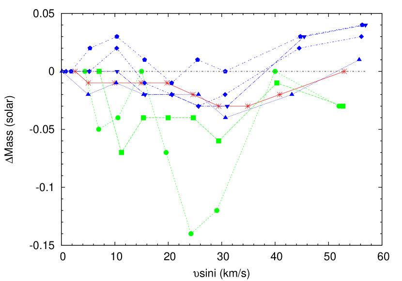
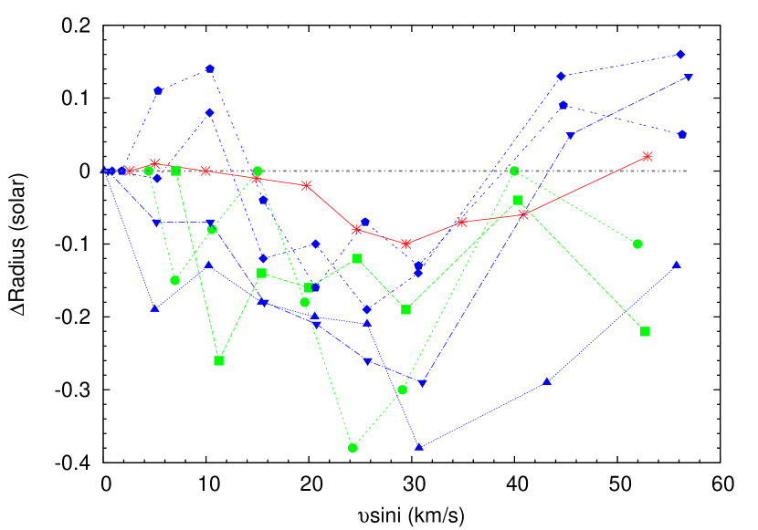
Figure 5: Differences in stellar mass (top panel) and radius (bottom panel) vs. $\upsilon\sin i$. The symbols are the same as in Fig. 4.

As $\upsilon\sin i$ increases, K-type stars show the highest differences in the stellar parameters compared to the non-broadened profile. These deviations for high $\upsilon\sin i$ are also shown in the error analysis of Sect. 2.4. The temperatures of these stars are systematically underestimated with increasing $\upsilon\sin i$. On the other hand, the parameters of F- and G-type stars are very close to the ones with slow rotation and no distinct trends are observed with rotation. Even for very high $\upsilon\sin i$, temperature and metallicitity can be derived with differences in values of less than 100 K and 0.05 dex respectively. Surface gravity, however, shows high differences that reach up to $\sim$0.20 dex.

The above discrepancies in the parameters affect in turn the stellar mass and radius. To investigate these offsets, we calculate the mass and radius for all the rotational velocities using the calibration of Torres et al. (2010) but corrected for small offsets to match masses derived from isochrone fits by Santos et al. (2013). The results in Fig. 5 show that the mass hardly changes as $\upsilon\sin i$ increases. Stellar radius however, is affected in the same manner as surface gravity with higher radius differences. For example, the maximum difference in $\log g$ ($\sim$0.20 dex) causes a deviation in radius of 0.39 R_⊙.

4.1 Application to FGK high rotators

We select a sample of FGK dwarfs with moderate/high $\upsilon\sin i$, that have available several estimates of their parameters from different techniques in the literature (see references in Table A.2). From these references, we included 17 stars with $\upsilon\sin i$ up to 54 km/s that have spectra available in the public archives of different high resolution instruments (HARPS, FEROS, ELODIE, and CORALIE). The spectra were already processed with their standard pipeline procedures. We corrected for the radial velocity shifts and in cases of multiple observations, the spectra are summed using the IRAF tools, dopcor and scombine respectively.

The stellar parameters are derived with the method of this work and the results and literature properties of the sample are presented in Table A.2. Table 5 shows the differences between the stellar parameters of this work and the different methods used: other spectral synthesis techniques, the EW method (until $\upsilon\sin i$ $\sim$ 10 km/s) and the photometric technique, namely IRFM. The differences between this work and other methods are very small for all parameters.

In Fig. 6 we plot the comparison between literature values and our results. Figure 7 shows the stellar parameters derived with different methods in dependence of rotational velocity from this work. Even though the mean differences in temperature are close to zero, there appears a slight overestimation of our method for high $\upsilon\sin i$. Surface gravity shows the lowest dispersion when compared to trigonometric $\log g$ from all methods. Metallicity is also in agreement, excluding perhaps an outlier (HD 49933).

Table 5: Differences in parameters derived with different methods. N indicates the number of stars used for the comparison.

	$\Delta T_{\mathrm{eff}}$ (K)	$\Delta\log g$ (dex)	$\Delta$ [Fe/H] (dex)	N
This Work – EW	3 $\pm$ 48	-0.11 $\pm$ 0.07	0.04 $\pm$ 0.03	11
	(MAD = 80)	(MAD = 0.24)	(MAD = 0.03)
This Work – Synthesis	32 $\pm$ 29	0.03 $\pm$ 0.05	0.05 $\pm$ 0.02	29
	(MAD = 64)	(MAD = 0.15)	(MAD = 0.04)
This Work – Photometry	-12 $\pm$ 25	0.06 $\pm$ 0.02	–	18
	(MAD = 44)	(MAD = 0.04)	–

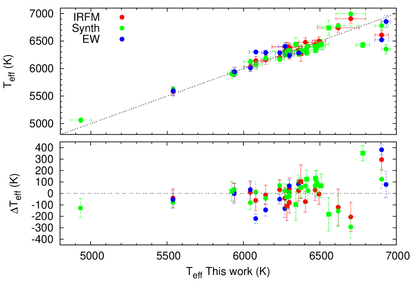
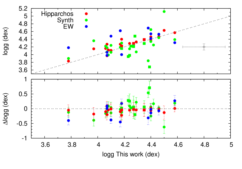
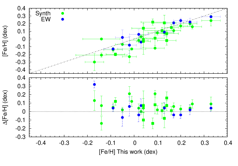
Figure 6: Temperature (top panel), surface gravity (middle panel), and metallicitity (bottom panel). Different colors represent different techniques. Square symbols represent planet-hosts analyzed in this work. In the middle panel, the average error is plotted. In each panel, the upper plot compares the data and the lower plot compares the residual differences from perfect agreement.

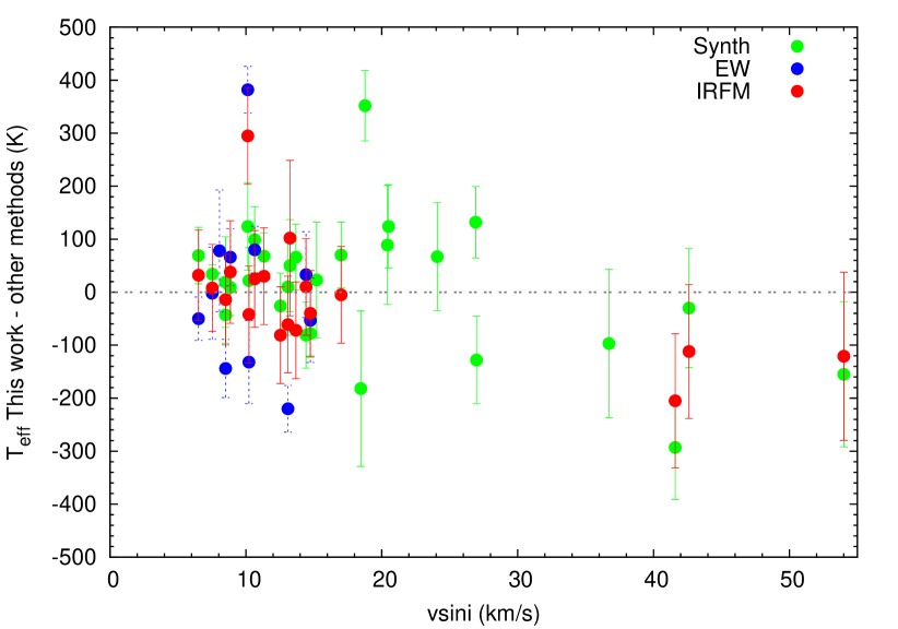
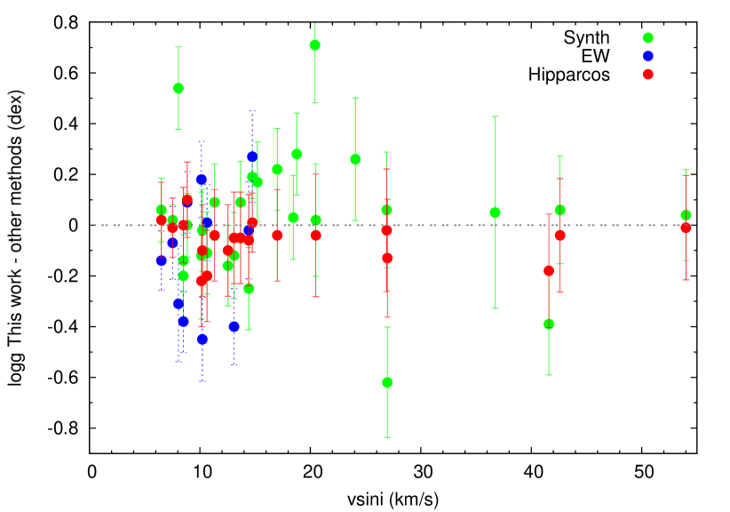
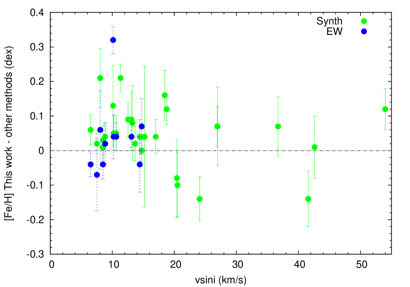
Figure 7: Differences in temperature (top panel), surface gravity (middle panel) and metallicitity (bottom panel) versus rotational velocity for moderate/high rotators.

5 Data and spectroscopic parameters for planet-hosts

We have identified spectra for 10 confirmed planet-hosts that show relatively high $\upsilon\sin i$ and we were unable to apply our standard EW method for their spectroscopic analysis. We use the procedure of this work to derive their stellar parameters to update the online SWEET-Cat catalogue where stellar parameters for FGK and M planet-hosts are presented (Santos et al. 2013). These stars were observed with high-resolution spectrographs (Table 6) gathered by our team (these spectra have never been analyzed before) and by the use of the archive (for the NARVAL spectra). Their spectral type varies from F to G.

The spectra were reduced with the standard pipelines and are corrected with the standard IRAF tools for the radial velocity shifts and in cases of multiple exposures of individual observed stars, their spectra are added. Following the procedure presented in this work, we derive their fundamental parameters, which are included in Figs. 6 and 7 (square symbols) and presented in Table 7. The stellar masses and radii are calculated using the calibration of Torres et al. (2010) with the corrections of Santos et al. (2013).

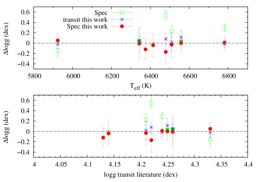
Figure 8: The differences refer to surface gravity derived from a transit light curve analysis minus other methods from Table 7. Circles correspond to the comparison of $\log g$ derived in this work. Squares correspond to the methodology applied by Valenti & Fischer (2005) and filled squares to other spectral synthesis methods. Asterisks show the comparison between $\log g$ derived from the light curve analysis on the literature and of this work.

Table 6: Observation log of the transit hosts analyzed in this work. V magnitudes are taken from SIMBAD. S/N is estimated at 6070 Å.

Star	V (mag)	Spectrograph	Resolution	S/N
30 Ari B	7.09	FEROS	48000	270
HAT-P-23	13.05	FEROS	48000	65
HAT-P-34	10.40	FEROS	48000	145
HAT-P-41	11.36	FEROS	48000	135
HAT-P-2	8.69	SOPHIE	75000	250
XO-3	9.85	SOPHIE	75000	130
HD 8673	6.31	NARVAL	75000	222
Kepler-410A	9.50	NARVAL	75000	72
CoRoT-11	12.80	HARPS	110000	116
CoRoT-3	13.29	HARPS	110000	84

Table 7: Spectroscopic parameters of planet-hosts derived in this work and surface gravities derived from the transit light curve are found in the literature for all transiting planet-hosts of our sample.

Star	$T_{\mathrm{eff}}$	$\log g$	$[Fe/H]$	$\upsilon\sin i$	$\log g_{transit}$	Ref.	Mass	Radius
	K	dex	dex	km/s	dex		M⊙	R⊙
HAT-P-23	5924 $\pm$ 30	4.28 $\pm$ 0.11	0.16 $\pm$ 0.03	8.50 $\pm$ 0.22	4.33 $\pm$ 0.05	(1)	1.13 $\pm$ 0.05	1.29 $\pm$ 0.05
Kepler-410A	6375 $\pm$ 44	4.25 $\pm$ 0.15	0.09 $\pm$ 0.04	13.24 $\pm$ 0.29	4.13 $\pm$ 0.11	(2)	1.30 $\pm$ 0.07	1.41 $\pm$ 0.07
CoRoT-3	6558 $\pm$ 44	4.25 $\pm$ 0.15	0.14 $\pm$ 0.04	18.46 $\pm$ 0.29	4.25 $\pm$ 0.07	(3)	1.41 $\pm$ 0.08	1.44 $\pm$ 0.08
XO-3	6781 $\pm$ 44	4.23 $\pm$ 0.15	-0.08 $\pm$ 0.04	18.77 $\pm$ 0.29	4.24 $\pm$ 0.04	(4)	1.41 $\pm$ 0.08	1.49 $\pm$ 0.08
HAT-P-41	6479 $\pm$ 51	4.39 $\pm$ 0.22	0.13 $\pm$ 0.05	20.11 $\pm$ 1.34	4.22 $\pm$ 0.07	(5)	1.28 $\pm$ 0.09	1.19 $\pm$ 0.08
HAT-P-2	6414 $\pm$ 51	4.18 $\pm$ 0.22	0.04 $\pm$ 0.05	20.50 $\pm$ 1.34	4.14 $\pm$ 0.03	(6)	1.34 $\pm$ 0.09	1.54 $\pm$ 0.12
HAT-P-34	6509 $\pm$ 51	4.24 $\pm$ 0.22	0.08 $\pm$ 0.05	24.08 $\pm$ 1.34	4.21 $\pm$ 0.06	(7)	1.36 $\pm$ 0.10	1.45 $\pm$ 0.11
HD 8673	6472 $\pm$ 51	4.27 $\pm$ 0.22	0.14 $\pm$ 0.05	26.91 $\pm$ 1.34	–	–	1.35 $\pm$ 0.10	1.39 $\pm$ 0.10
CoRoT-11	6343 $\pm$ 72	4.27 $\pm$ 0.30	0.04 $\pm$ 0.03	36.72 $\pm$ 1.34	4.26 $\pm$ 0.06	(8)	1.56 $\pm$ 0.10	1.36 $\pm$ 0.13
30 Ari B	6284 $\pm$ 98	4.35 $\pm$ 0.20	0.12 $\pm$ 0.08	42.61 $\pm$ 1.82	–	–	1.22 $\pm$ 0.08	1.23 $\pm$ 0.07

(1) Bakos et al. (2011); (2) Van Eylen et al. (2014); (3) Deleuil et al. (2008); (4) Johns-Krull et al. (2008); (5) Hartman et al. (2012); (6) Pál et al. (2010); (7) Bakos et al. (2012); (8) Gandolfi et al. (2010)

Table 8: Transit fit parameters

Name	Rp/R⋆	Td	$\rho_{\star}$	g1
		days	g cm-3
HAT-P-23	0.1209${}_{-0.0011}^{+0.0015}$	0.0822${}_{-0.0008}^{+0.0005}$	0.976${}_{-0.102}^{+0.068}$	0.281${}_{-0.056}^{+0.037}$
HAT-P-34	0.0842${}_{-0.0015}^{+0.0015}$	0.1323${}_{-0.0015}^{+0.0013}$	0.505${}_{-0.119}^{+0.097}$	0.037${}_{-0.019}^{+0.111}$
HAT-P-41	0.1049${}_{-0.0004}^{+0.0011}$	0.1523${}_{-0.0009}^{+0.0004}$	0.452${}_{-0.054}^{+0.003}$	0.211${}_{-0.044}^{+0.019}$
XO-3	0.0915${}_{-0.0007}^{+0.0006}$	0.1043${}_{-0.0008}^{+0.0010}$	0.649${}_{-0.060}^{+0.060}$	0.343${}_{-0.090}^{+0.030}$
CoRoT-3	0.0641${}_{-0.0005}^{+0.0007}$	0.1410${}_{-0.0008}^{+0.0010}$	0.431${}_{-0.055}^{+0.074}$	0.202${}_{-0.062}^{+0.041}$
CoRoT-11	0.0999${}_{-0.0005}^{+0.0006}$	0.0799${}_{-0.0012}^{+0.0010}$	0.581${}_{-0.023}^{+0.034}$	0.347${}_{-0.092}^{+0.062}$

5.1 Transit analysis

We retrieve from the literature available photometric data for our transiting planet target stars. Our aim is to perform an homogeneous analysis of these objects using our re-determined stellar parameters to guess limb darkening coefficients and average stellar density. The limb darkening coefficients are linearly interpolated in the 4 dimension of the new stellar parameters ($T_{\mathrm{eff}}$, $\log g$, $[Fe/H]$, and $\upsilon_{mac}$) from the tables of Claret & Bloemen (2011) to match our stellar parameter values. We obtain as well the stellar density from the mass and radius as described in the previous Section. Transit duration and transit depth are initially taken from the values quoted in the literature. The light curves are all folded with the period known from the literature and out of transit measurements are normalized to one.

Since some of the planets in our sample are in eccentric orbits, we adopt the expansion to the fourth order for the normalized projected distance of the planet with respect to the stellar center reported in Pál et al. (2010) and express it as a function of the stellar density ($\rho_{\star}$) and the transit duration ($T_{d}$).

For each folded light curve, we fit a transiting planet model using the Mandel & Agol (2002) model and the Levemberg-Marquardt algorithm (Press et al. 1992). For eccentric planets we adopt the values of the eccentricity and argument of periastron reported in the literature and add a gaussian prior on both during our error analysis (see below) considering the reported uncertainties.

The uncertainties of the measurements are first expanded by the reduced $\chi^{2}$ of the fit. We account for correlated noise creating a mock sample of the fit residuals (using the measurement uncertainties) and comparing the scatter in the artificial and in the real light curves re-binning the residuals on increasing time-intervals (up to 30 min). If the ratio of the expected to the real scatter is found larger than one, we further expanded the uncertainties by this factor. Finally, we determine the distributions of the parameter best-fit values bootstrapping the light curves and derived the mode of the resulting distributions, and the 68.3 per cent confidence limits defined by the 15.85th and the 84.15th percentiles in the cumulative distributions.

The results are reported in Table 8. The photometric densities appear smaller than the values implied by theoretical models. The discrepancy is largest for the case of Kepler-410A where models predict $\rho_{\star}\sim 1\,$g cm^-3, whereas the measured value is 0.0937${}_{-0.0052}^{+0.0070}$ g cm^-3. The dilution caused by the contamination of a stellar companion (Kepler-410B) and the small size of the planet (2.838 R_⊕, Van Eylen et al. (2014)) are the main reasons for the difference in the density derived from the transit fit. Considering the above, we exclude this star from the comparison of the transit fit results.

5.2 Discussion

For stars with a transiting planet, surface gravity has been proposed to be independently derived from the light curve with better precision than from spectroscopy (Seager & Mallén-Ornelas 2003; Sozzetti et al. 2007). In Torres et al. (2012), it has been shown that $\log g$ derived using SME and the methodology of Valenti & Fischer (2005) is systematically underestimated for hotter stars ($T_{\mathrm{eff}}>$ 6000 K) when compared with the $\log g$ from transit fits. According to the authors, constraining $\log g$ to the transit values, as more reliable, leads to significant biases in the temperature and metallicitity which consequently propagates to biases in stellar (and planetary) mass and radius.

From the planet-hosts in our work, there are 8 stars with transit data and available $\log g$ using a light curve analysis. We therefore, compare the $\log g$ derived from our spectroscopic analysis with the $\log g$ from the transit fits as taken from the literature (red circles in Fig. 8). The differences of this comparison are very small ($\Delta\log g$ = -0.04  with $\sigma$= 0.07 dex). On the other hand, a comparison between the $\log g$ from the transit light curve and the $\log g$ using only the unconstrained Valenti & Fischer (2005) methodology shows difference of 0.18 ($\sigma$= 0.27) dex for 5 stars with available measurements (empty squares in Fig. 8). We also plot for completeness the $\log g$ from our light curve analysis of the previous Section, using the stellar density and mass (asterisks in Fig. 8).

Even though the number of stars for this comparison is very small, these results suggest that fixing $\log g$ to the transit value is not required with the analysis of this work, avoiding the biases that are described in Torres et al. (2012). The different approach we adopt in this work, mainly due to the different line list, shows that we obtain a better estimate on surface gravity. However, since our sample is small and limited only to hotter stars, further investigation is advised to check whether following the unconstrained approach is the optimal strategy. The unconstrained analysis is also suggested in Gómez Maqueo Chew et al. (2013) as preferred, after analyzing the transit-host WASP-13 with SME but following different methodology (line list, initial parameters, convergence criteria, fixed parameters) from Valenti & Fischer (2005).

Figure 9: Comparison between the literature data of planetary mass, the radii ratio (R_p/R_star), and planetary radius and this work, respectively in absolute units.

We explore how the literature values of planetary mass and radius are affected with the new stellar parameters. From our analysis we find that the dispersion between the planetary mass derived with our stellar parameters and the literature is 4% (Fig. 9, top panel). The planet-to-star radius ratio derived from the transit light curve shows same dispersion of 4% (Fig. 9, middle panel). This consistency with the literature values confirms the accuracy of the transit light curve analysis to derive planet-to-star radius ratio. The planetary radius is calculated from this ratio and the stellar radius that is inferred from our spectroscopic values. The comparison of the planetary radius with the literature values shows the highest dispersion of 14% (Fig. 9, bottom panel). Since we have shown the consistency of the planet-to-star radius ratio, the main source of uncertainty in the derivation of planetary radius is the calculation of the stellar value.

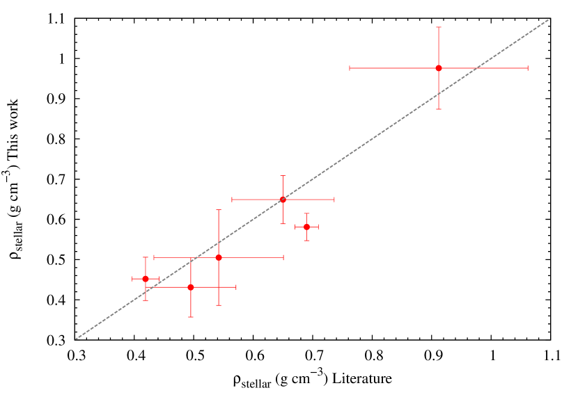
Figure 10: Comparison between stellar density derived from the transit light curve analysis and literature data.

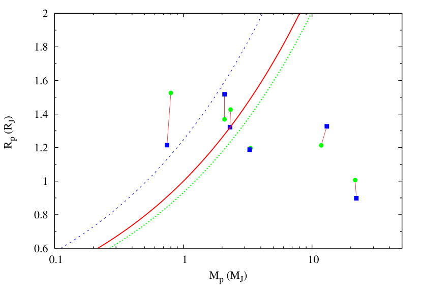
Figure 11: Blue squares represent planetary mass and radius derived in this work in comparison with literature values (green circles). Characteristic isodensity curves are plotted for Saturn (dashed), Jupiter (solid) and Neptune (dotted).

We also compare the stellar density derived from the transit analysis with the respective ones from the literature (Fig. 10). In Fig. 11, we show the new mass and radius from this work in comparison with the literature values. Planetary radius shows higher discrepancies mainly because of the uncertainties in the stellar radius calculations.

6 Conclusions

In this paper we are introducing a new approach for the derivation of the fundamental stellar parameters for FGK dwarfs using the spectral synthesis technique. In particular, we focus on stars with moderate/high rotational velocities. Such stars could be transiting planet-hosts as they show high dispersion in their rotational velocities and the determination of their stellar parameters is of principal importance for the planetary studies.

The key of our method is the selection of the line list that contains principally iron lines based on previous work. This line list is tested primarily for stars with low rotational velocities. The comparison in temperatures between the EW method and this work for our test sample is in good agreement even though high temperatures ($T_{\mathrm{eff}}>$ 6000 K) are underestimated by the synthesis technique. Metallicity is in excellent agreement with our test sample and surface gravity shows an offset of -0.19 dex.

Our method is applied to reference stars that are convolved with a set of rotational profiles (up to $\upsilon\sin i$ = 50 km/s). The spectrum of each reference star has been broadened with different $\upsilon\sin i$ values and for these spectra we calculate the stellar parameters which are compared with the initial unbroadened spectrum in order to check their consistency for high $\upsilon\sin i$. The results show that even for high $\upsilon\sin i$ the differences from the ones without broadening is on the same scale as the errors.

As a final test we calculate stellar parameters for a sample of stars with high $\upsilon\sin i$ and compare with other spectral synthesis methodologies, the EW method (when possible), and the IRFM. The comparison shows very good agreement with all methods with the same dispersion in the mean differences of the parameters as the slow rotating stars.

We also applied our method to 10 planet-hosts with moderate/high rotation, updating their stellar parameters in a uniform way. A new analysis has been conducted to the light curves for the stars that had available photometric observations using our results. From the combination of spectroscopic parameters and the ones derived from the transit fits (namely stellar density), we calculate surface gravity and the comparison with spectroscopic derivations suggests that fixing $\log g$ to the transit value is not required using our method. In addition, we present the difference in the planetary mass and radius (expressed as a percentage) with the literature values. Planetary masses agree very well with the literature values. The dispersion in the radii of the planets is higher due to larger errors in the estimation of the stellar radius.

The study of planet-hosts with higher rotational velocities is essential because they expand the planet sample around stars of earlier types (F- and A-type) that are more massive than the Sun. Precise stellar parameters for these stars are necessary to study the frequency of planets around intermediate mass stars and explore their planet formation mechanisms. Additionally, precise (and if possible accurate) stellar parameters are essential for a detailed characterization of the planets to be discovered by the upcoming high precision transit missions such as CHEOPS, TESS, and PLATO 2.0.

Appendix A

Table 9: Results of the comparison between this work and the EW method. The stars in boldface are analyzed in Sect. 4.

	This work				EW method
Star	$T_{\mathrm{eff}}$	$\log g$	[Fe/H]	$\upsilon\sin i$	$T_{\mathrm{eff}}$	$\log g$	[Fe/H]
	(K)	(dex)	(dex)	(km/s)	(K)	(dex)	(dex)
Dwarf stars
CoRoT-2	5620 $\pm$ 18	4.66 $\pm$ 0.06	-0.03 $\pm$ 0.03	9.97	5697 $\pm$ 97	4.73 $\pm$ 0.17	-0.09 $\pm$ 0.07
CoRoT-10	4921 $\pm$ 25	4.09 $\pm$ 0.09	0.15 $\pm$ 0.03	2.19	5025 $\pm$ 155	4.47 $\pm$ 0.31	0.06 $\pm$ 0.09
CoRoT-4	6164 $\pm$ 30	4.34 $\pm$ 0.11	0.15 $\pm$ 0.03	7.03	6344 $\pm$ 93	4.82 $\pm$ 0.11	0.15 $\pm$ 0.06
CoRoT-5	6254 $\pm$ 30	4.41 $\pm$ 0.11	0.04 $\pm$ 0.03	1.43	6240 $\pm$ 70	4.46 $\pm$ 0.11	0.04 $\pm$ 0.05
HD 101930	5083 $\pm$ 18	4.15 $\pm$ 0.06	0.10 $\pm$ 0.03	0.10	5083 $\pm$ 63	4.35 $\pm$ 0.13	0.16 $\pm$ 0.04
HD 102365	5588 $\pm$ 18	4.07 $\pm$ 0.06	-0.30 $\pm$ 0.03	0.10	5616 $\pm$ 41	4.40 $\pm$ 0.06	-0.28 $\pm$ 0.03
HD 103774	6582 $\pm$ 30	4.47 $\pm$ 0.11	0.27 $\pm$ 0.03	8.93	6732 $\pm$ 56	4.81 $\pm$ 0.06	0.29 $\pm$ 0.03
HD 1237	5588 $\pm$ 18	4.58 $\pm$ 0.06	0.11 $\pm$ 0.03	4.62	5489 $\pm$ 40	4.46 $\pm$ 0.11	0.06 $\pm$ 0.03
HD 134060	5914 $\pm$ 18	4.28 $\pm$ 0.06	0.09 $\pm$ 0.03	1.44	5940 $\pm$ 18	4.42 $\pm$ 0.03	0.12 $\pm$ 0.01
HD 1388	5967 $\pm$ 18	4.38 $\pm$ 0.06	0.00 $\pm$ 0.03	1.27	5970 $\pm$ 15	4.42 $\pm$ 0.05	0.00 $\pm$ 0.01
HD 148156	6212 $\pm$ 30	4.40 $\pm$ 0.11	0.23 $\pm$ 0.03	5.73	6251 $\pm$ 25	4.51 $\pm$ 0.05	0.25 $\pm$ 0.02
HD 162020	4798 $\pm$ 25	4.14 $\pm$ 0.09	-0.14 $\pm$ 0.03	1.46	4723 $\pm$ 71	4.31 $\pm$ 0.18	-0.10 $\pm$ 0.03
HD 20852	6675 $\pm$ 30	4.12 $\pm$ 0.11	-0.37 $\pm$ 0.03	7.06	6813 $\pm$ 92	4.76 $\pm$ 0.12	-0.35 $\pm$ 0.06
HD 20868	4745 $\pm$ 25	4.02 $\pm$ 0.09	0.00 $\pm$ 0.03	0.46	4720 $\pm$ 91	4.24 $\pm$ 0.47	0.08 $\pm$ 0.01
HD 221287	6337 $\pm$ 30	4.43 $\pm$ 0.06	0.02 $\pm$ 0.06	3.92	6417 $\pm$ 25	4.60 $\pm$ 0.10	0.06 $\pm$ 0.02
HD 222237	4618 $\pm$ 25	3.92 $\pm$ 0.09	-0.50 $\pm$ 0.03	0.10	4722 $\pm$ 55	4.34 $\pm$ 0.15	-0.39 $\pm$ 0.06
HD 23079	5965 $\pm$ 18	4.28 $\pm$ 0.06	-0.13 $\pm$ 0.03	0.10	6009 $\pm$ 14	4.50 $\pm$ 0.05	-0.11 $\pm$ 0.01
HD 27894	4894 $\pm$ 25	4.08 $\pm$ 0.09	0.18 $\pm$ 0.03	0.87	4833 $\pm$ 209	4.30 $\pm$ 0.48	0.26 $\pm$ 0.10
HD 31527	5915 $\pm$ 18	4.40 $\pm$ 0.06	-0.17 $\pm$ 0.03	2.36	5917 $\pm$ 13	4.47 $\pm$ 0.05	-0.17 $\pm$ 0.01
HD 330075	4924 $\pm$ 30	4.03 $\pm$ 0.09	-0.04 $\pm$ 0.03	0.10	4958 $\pm$ 52	4.24 $\pm$ 0.13	0.05 $\pm$ 0.03
HD 361	5924 $\pm$ 18	4.48 $\pm$ 0.06	-0.10 $\pm$ 0.03	0.10	5888 $\pm$ 14	4.54 $\pm$ 0.08	-0.13 $\pm$ 0.01
HD 38283	5962 $\pm$ 18	4.14 $\pm$ 0.06	-0.15 $\pm$ 0.03	4.51	5980 $\pm$ 24	4.27 $\pm$ 0.03	-0.14 $\pm$ 0.02
HD 40307	4771 $\pm$ 25	4.10 $\pm$ 0.09	-0.42 $\pm$ 0.03	0.10	4774 $\pm$ 77	4.42 $\pm$ 0.16	-0.36 $\pm$ 0.02
HD 61421	6616 $\pm$ 30	4.09 $\pm$ 0.11	0.03 $\pm$ 0.03	4.40	6612	4.02	-0.02
HD 63454	4833 $\pm$ 25	4.11 $\pm$ 0.09	0.04 $\pm$ 0.03	1.81	4756 $\pm$ 77	4.32 $\pm$ 0.22	0.13 $\pm$ 0.05
HD 750	5118 $\pm$ 18	4.34 $\pm$ 0.06	-0.29 $\pm$ 0.03	0.10	5069 $\pm$ 32	4.33 $\pm$ 0.1	-0.30 $\pm$ 0.02
HD 870	5379 $\pm$ 18	4.36 $\pm$ 0.06	-0.12 $\pm$ 0.03	0.10	5360 $\pm$ 24	4.40 $\pm$ 0.08	-0.12 $\pm$ 0.02
HD 93385	5987 $\pm$ 18	4.38 $\pm$ 0.06	0.02 $\pm$ 0.03	1.06	5989 $\pm$ 17	4.46 $\pm$ 0.03	0.03 $\pm$ 0.01
HD 967	5643 $\pm$ 18	4.38 $\pm$ 0.06	-0.59 $\pm$ 0.03	0.10	5595 $\pm$ 18	4.59 $\pm$ 0.02	-0.66 $\pm$ 0.01
OGLE-TR-113	4793 $\pm$ 25	4.25 $\pm$ 0.09	0.05 $\pm$ 0.03	5.02	4781 $\pm$ 166	4.31 $\pm$ 0.41	0.03 $\pm$ 0.06
WASP-29	4782 $\pm$ 25	4.13 $\pm$ 0.09	0.18 $\pm$ 0.03	0.10	5203 $\pm$ 102	4.93 $\pm$ 0.21	0.17 $\pm$ 0.05
WASP-15	6378 $\pm$ 30	4.24 $\pm$ 0.11	0.03 $\pm$ 0.03	5.13	6573 $\pm$ 70	4.79 $\pm$ 0.08	0.09 $\pm$ 0.03
WASP-16	5710 $\pm$ 18	4.23 $\pm$ 0.06	0.12 $\pm$ 0.03	0.47	5726 $\pm$ 22	4.34 $\pm$ 0.05	0.13 $\pm$ 0.02
WASP-17	6666 $\pm$ 30	4.26 $\pm$ 0.06	-0.04 $\pm$ 0.03	9.93	6794 $\pm$ 83	4.83 $\pm$ 0.09	-0.12 $\pm$ 0.05
WASP-2	5105 $\pm$ 18	3.97 $\pm$ 0.06	0.08 $\pm$ 0.03	2.90	5109 $\pm$ 72	4.33 $\pm$ 0.14	0.02 $\pm$ 0.05
WASP-23	5053 $\pm$ 18	4.20 $\pm$ 0.06	-0.02 $\pm$ 0.03	0.46	5046 $\pm$ 99	4.33 $\pm$ 0.18	0.05 $\pm$ 0.06
WASP-38	6247 $\pm$ 30	4.25 $\pm$ 0.11	0.06 $\pm$ 0.03	8.05	6436 $\pm$ 60	4.80 $\pm$ 0.07	0.06 $\pm$ 0.04
WASP-6	5447 $\pm$ 18	4.42 $\pm$ 0.06	-0.11 $\pm$ 0.03	0.10	5383 $\pm$ 41	4.52 $\pm$ 0.06	-0.14 $\pm$ 0.03
Sun	5771 $\pm$ 18	4.42 $\pm$ 0.06	0.00 $\pm$ 0.03	2.57	–	–	–
Giant stars
HD 148427	5018 $\pm$ 25	3.49 $\pm$ 0.09	0.01 $\pm$ 0.03	0.45	4962 $\pm$ 45	3.39 $\pm$ 0.12	0.03 $\pm$ 0.03
HD 175541	5097 $\pm$ 18	3.44 $\pm$ 0.06	-0.14 $\pm$ 0.03	2.45	5111 $\pm$ 38	3.56 $\pm$ 0.08	-0.11 $\pm$ 0.03
HD 27442	4852 $\pm$ 25	3.48 $\pm$ 0.09	0.23 $\pm$ 0.03	2.65	4781 $\pm$ 76	3.46 $\pm$ 0.19	0.33 $\pm$ 0.05
HD 62509	5007 $\pm$ 25	3.06 $\pm$ 0.09	0.21 $\pm$ 0.03	3.76	4935 $\pm$ 49	2.91 $\pm$ 0.13	0.09 $\pm$ 0.04
HD 88133	5330 $\pm$ 18	3.62 $\pm$ 0.06	0.20 $\pm$ 0.03	3.39	5438 $\pm$ 34	3.94 $\pm$ 0.11	0.33 $\pm$ 0.05
HD 142091	4898 $\pm$ 25	3.24 $\pm$ 0.09	0.05 $\pm$ 0.03	4.38	4876 $\pm$ 46	3.15 $\pm$ 0.14	0.13 $\pm$ 0.03
HD 188310	4799 $\pm$ 18	3.14 $\pm$ 0.06	-0.06 $\pm$ 0.03	5.28	4714 $\pm$ 49	2.53 $\pm$ 0.11	-0.27 $\pm$ 0.04
HD 163917	5107 $\pm$ 18	2.82 $\pm$ 0.06	0.33 $\pm$ 0.03	4.21	4967 $\pm$ 61	2.70 $\pm$ 0.13	0.14 $\pm$ 0.05

Table 10: Stellar parameters for a sample of high rotating FGK dwarfs.

Star	$T_{\mathrm{eff}IRFM}$	Ref.	$\log g_{HIP}$	$T_{\mathrm{eff}}$	$\log g$	$[Fe/H]$	Ref.	$T_{\mathrm{eff}Synth}$	$\log g_{Synth}$	$[Fe/H]_{Synth}$	Ref.	$T_{\mathrm{eff}EW}$	$\log g_{EW}$	$[Fe/H]_{EW}$	Ref.	$\upsilon\sin i$
	K		dex	K	dex	dex		K	dex	dex		K	dex	dex		km/s
HD 179949	6205 $\pm$ 80	(1)	4.38 $\pm$ 0.10	6237 $\pm$ 30	4.40 $\pm$ 0.11	0.17 $\pm$ 0.03	This work	6168 $\pm$ 44	4.34 $\pm$ 0.06	0.11 $\pm$ 0.03	(3)	6287 $\pm$ 28	4.54 $\pm$ 0.04	0.21 $\pm$ 0.02	18	6.52
HD 165185	5932 $\pm$ 80	(1)	4.47 $\pm$ 0.10	5940 $\pm$ 18	4.46 $\pm$ 0.06	-0.05 $\pm$ 0.03	This work	5906	4.44	-0.07	(4)	5942 $\pm$ 85	4.53 $\pm$ 0.13	0.02 $\pm$ 0.10	19	7.53
HAT-P-6	–	–	–	6933 $\pm$ 30	4.38 $\pm$ 0.11	-0.02 $\pm$ 0.03	This work	6353 $\pm$ 88	3.84 $\pm$ 0.12	-0.23 $\pm$ 0.08	(5)	6855 $\pm$ 111	4.69 $\pm$ 0.20	-0.08 $\pm$ 0.11	20	8.06
HAT-P-23	–	–	–	5924 $\pm$ 30	4.28 $\pm$ 0.11	0.16 $\pm$ 0.03	This work	5905 $\pm$ 80	4.48 $\pm$ 0.12	0.15 $\pm$ 0.04	(10)	–	–	–	–	8.50
HD 19994	6159 $\pm$ 80	(1)	4.10 $\pm$ 0.10	6145 $\pm$ 30	4.10 $\pm$ 0.11	0.20 $\pm$ 0.03	This work	6188 $\pm$ 44	4.24 $\pm$ 0.06	0.17 $\pm$ 0.03	(3)	6289 $\pm$ 46	4.48 $\pm$ 0.05	0.24 $\pm$ 0.03	18	8.51
HD 89744	6262 $\pm$ 92	(1)	3.97 $\pm$ 0.10	6300 $\pm$ 30	4.07 $\pm$ 0.11	0.24 $\pm$ 0.03	This work	6291 $\pm$ 44	4.07 $\pm$ 0.06	0.20 $\pm$ 0.03	(3)	6234 $\pm$ 45	3.98 $\pm$ 0.05	0.22 $\pm$ 0.05	21	8.86
HD 49933	6609 $\pm$ 80	(1)	4.40 $\pm$ 0.10	6904 $\pm$ 44	4.18 $\pm$ 0.15	-0.17 $\pm$ 0.04	This work	6780 $\pm$ 70	4.30 $\pm$ 0.20	-0.30 $\pm$ 0.11	(6)	6522	4.00	-0.49	22	10.14
HD 142	6313 $\pm$ 80	(1)	4.27 $\pm$ 0.10	6271 $\pm$ 44	4.17 $\pm$ 0.15	0.13 $\pm$ 0.04	This work	6249 $\pm$ 44	4.19 $\pm$ 0.06	0.08 $\pm$ 0.03	(3)	6403 $\pm$ 65	4.62 $\pm$ 0.07	0.09 $\pm$ 0.05	18	10.22
HD 142860	6336 $\pm$ 80	(1)	4.27 $\pm$ 0.10	6361 $\pm$ 44	4.07 $\pm$ 0.15	-0.09 $\pm$ 0.04	This work	6262 $\pm$ 44	4.18 $\pm$ 0.06	-0.14 $\pm$ 0.03	(3)	6281	4.06	-0.13	22	10.65
HD 89569	6439 $\pm$ 80	(1)	4.12 $\pm$ 0.10	6469 $\pm$ 44	4.08 $\pm$ 0.15	0.09 $\pm$ 0.04	This work	6401	3.99	-0.12	(4)	–	–	–	–	11.33
HD 86264	6381 $\pm$ 80	(1)	4.16 $\pm$ 0.10	6300 $\pm$ 44	4.06 $\pm$ 0.15	0.25 $\pm$ 0.04	This work	6326 $\pm$ 44	4.22 $\pm$ 0.05	0.16 $\pm$ 0.03	(3)	6596 $\pm$ 78	4.47 $\pm$ 0.15	0.37 $\pm$ 0.06	23	12.55
HD 121370	6141 $\pm$ 80	(1)	3.83 $\pm$ 0.10	6080 $\pm$ 44	3.78 $\pm$ 0.15	0.33 $\pm$ 0.04	This work	6030 $\pm$ 80	3.90 $\pm$ 0.08	0.24 $\pm$ 0.07	(7)	6300	4.18	0.29	22	13.10
Kepler-410A	6273 $\pm$ 140	(2)	–	6375 $\pm$ 44	4.25 $\pm$ 0.15	0.09 $\pm$ 0.04	This work	6325 $\pm$ 75	–	0.01 $\pm$ 0.10	8	–	–	–	–	13.24
HD 210302	6477 $\pm$ 80	(1)	4.29 $\pm$ 0.10	6405 $\pm$ 44	4.24 $\pm$ 0.15	0.10 $\pm$ 0.04	This work	6339 $\pm$ 44	4.15 $\pm$ 0.06	0.08 $\pm$ 0.03	(3)	–	–	–	–	13.68
HD 105	6035 $\pm$ 80	(1)	4.46 $\pm$ 0.10	6045 $\pm$ 44	4.40 $\pm$ 0.15	0.02 $\pm$ 0.04	This work	6126 $\pm$ 44	4.65 $\pm$ 0.06	-0.02 $\pm$ 0.03	(3)	6012 $\pm$ 68	4.42 $\pm$ 0.12	0.06 $\pm$ 0.07	24	14.43
HD 202917	5579 $\pm$ 80	(1)	4.57 $\pm$ 0.10	5539 $\pm$ 10	4.58 $\pm$ 0.06	0.03 $\pm$ 0.01	This work	5617 $\pm$ 44	4.39 $\pm$ 0.06	0.03 $\pm$ 0.03	(3)	5592 $\pm$ 79	4.31 $\pm$ 0.17	-0.04 $\pm$ 0.08	24	14.75
WASP-3	–	–	–	6423 $\pm$ 44	4.42 $\pm$ 0.15	0.04 $\pm$ 0.04	This work	6400 $\pm$ 100	4.25 $\pm$ 0.05	0.00 $\pm$ 0.20	(9)	6448 $\pm$ 123	4.49 $\pm$ 0.08	-0.02 $\pm$ 0.08	25	15.21
HD 30652	6499 $\pm$ 80	(1)	4.33 $\pm$ 0.10	6494 $\pm$ 44	4.29 $\pm$ 0.15	0.04 $\pm$ 0.04	This work	6424 $\pm$ 44	4.07 $\pm$ 0.06	0.00 $\pm$ 0.03	(3)	–	–	–	–	17.01
CoRoT-3	–	–	–	6558 $\pm$ 44	4.25 $\pm$ 0.15	0.14 $\pm$ 0.04	This work	6740 $\pm$ 140	4.22 $\pm$ 0.07	-0.02 $\pm$ 0.06	(11)	–	–	–	–	18.46
XO-3	–	–	–	6781 $\pm$ 44	4.23 $\pm$ 0.15	-0.08 $\pm$ 0.04	This work	6429 $\pm$ 50	3.95 $\pm$ 0.06	-0.20 $\pm$ 0.02	(12)	–	–	–	–	18.77
HAT-P-41	–	–	–	6479 $\pm$ 51	4.39 $\pm$ 0.22	0.13 $\pm$ 0.05	This work	6390 $\pm$ 100	3.68 $\pm$ 0.06	0.21 $\pm$ 0.10	(13)	–	–	–	–	20.11
HAT-P-2	–	–	4.22 $\pm$ 0.10	6414 $\pm$ 51	4.18 $\pm$ 0.22	0.04 $\pm$ 0.05	This work	6290 $\pm$ 60	4.16 $\pm$ 0.03	0.14 $\pm$ 0.08	(14)	–	–	–	–	20.50
HAT-P-34	–	–	–	6509 $\pm$ 51	4.24 $\pm$ 0.22	0.08 $\pm$ 0.05	This work	6442 $\pm$ 88	3.98 $\pm$ 0.10	0.22 $\pm$ 0.04	(15)	–	–	–	–	24.08
HD 8673	–	–	4.29 $\pm$ 0.10	6472 $\pm$ 51	4.27 $\pm$ 0.22	0.14 $\pm$ 0.05	This work	6340 $\pm$ 44	4.21 $\pm$ 0.06	0.07 $\pm$ 0.03	(3)	–	–	–	–	26.91
HD 82558	–	–	4.63 $\pm$ 0.11	4934 $\pm$ 70	4.50 $\pm$ 0.21	-0.14 $\pm$ 0.11	This work	5062 $\pm$ 44	5.12 $\pm$ 0.06	-0.21 $\pm$ 0.03	(3)	–	–	–	–	26.97
CoRoT-11	–	–	–	6343 $\pm$ 72	4.27 $\pm$ 0.30	0.04 $\pm$ 0.03	This work	6440 $\pm$ 120	4.22 $\pm$ 0.23	-0.03 $\pm$ 0.08	(16)	–	–	–	–	36.72
HD 64685	6907 $\pm$ 80	(1)	4.15 $\pm$ 0.12	6702 $\pm$ 98	3.97 $\pm$ 0.20	-0.14 $\pm$ 0.08	This work	6995	4.36	0.00	4	–	–	–	–	41.59
30 Ari B	6396 $\pm$ 80	(1)	4.39 $\pm$ 0.12	6284 $\pm$ 60	4.35 $\pm$ 0.25	0.12 $\pm$ 0.06	This work	6314 $\pm$ 55	4.29 $\pm$ 0.07	0.11 $\pm$ 0.04	(17)	–	–	–	–	42.61
HD 219877	6741 $\pm$ 80	(1)	4.11 $\pm$ 0.13	6620 $\pm$ 137	4.10 $\pm$ 0.18	-0.01 $\pm$ 0.06	This work	6775	4.06	-0.13	4	–	–	–	–	54.00