Supernova 2010as: the Lowest-Velocity Member of a Family of Flat-Velocity Type IIb Supernovae

Abstract

We present extensive optical and near-infrared photometric and spectroscopic observations of the stripped-envelope (SE) supernova SN 2010as. Spectroscopic peculiarities, such as initially weak helium features and low expansion velocities with a nearly flat evolution, place this object in the small family of events previously identified as transitional Type Ib/c supernovae (SNe). There is ubiquitous evidence of hydrogen, albeit weak, in this family of SNe, indicating that they are in fact a peculiar kind of Type IIb SNe that we name “flat-velocity Type IIb”. The flat velocity evolution—which occurs at different levels between 6000 and 8000 km s^-1 for different SNe—suggests the presence of a dense shell in the ejecta. Despite the spectroscopic similarities, these objects show surprisingly diverse luminosities. We discuss the possible physical or geometrical unification picture for such diversity. Using archival HST images we associate SN 2010as with a massive cluster and derive a progenitor age of $\approx$6 Myr, assuming a single star-formation burst, which is compatible with a Wolf-Rayet progenitor. Our hydrodynamical modelling, on the contrary, indicates the pre-explosion mass was relatively low, of $\approx$4 $M_{\odot}$. The seeming contradiction between an young age and low pre-SN mass may be solved by a massive interacting binary progenitor.

1. INTRODUCTION

Stripped-envelope supernovae (SE SNe)—i.e., those with hydrogen-poor spectra—are observationally very diverse. This somewhat loosely defined group comprises H-poor Type IIb SNe, H-deficient and He-rich Type Ib SNe, and both H- and He-deficient Type Ic SNe. While it is established that most of these events arise from the core collapse of massive stars (with initial masses above 8 $M_{\odot}$), we lack a clear knowledge concerning the connection between different subtypes and stellar progenitors or explosion processes. In particular, there is the long-standing question of how stars get rid of their outer envelopes before exploding. Is it through strong winds, by eruptive episodes like in luminous blue variable stars, by mass transfer in close binary systems, or are there other mechanisms at play (see, e.g., Langer, 2012)? Is there a distinct separation between Type Ib and Type IIb SNe, or is it a continuum regulated by the amount of hydrogen (Nomoto et al., 1995; Heger et al., 2003; Georgy et al., 2009; Yoon et al., 2010)? What is the reason for Type Ic SNe not to show helium in the spectra (Hachinger et al., 2012; Dessart et al., 2012a)? Theory and observation can help each other to solve these issues and thereby provide a more physically motivated subdivision of SE SN types.

Some pieces of the puzzle can be sought for in the increasing amount of events intensively observed soon after explosion. For instance, this has led to the discovery of SNe with observational properties in between the subtype definitions. Of particular interest among these is a small group of SNe with spectroscopic characteristics that drift from Type Ic to Type Ib as helium lines become more prevalent with phase. This sort of behavior was first identified for SN 1999ex (Hamuy et al., 2002), and a subclass of intermediate or transitional Type Ib/c was introduced. The term transitional is used here to distinguish this classification from a loose “Type Ibc” class that is sometimes used to indicate that the SN could either be Type Ib or Type Ic. Similar cases were subsequently found, such as SN 2005bf (Anupama et al., 2005; Tominaga et al., 2005; Folatelli et al., 2006), SN 2007Y (Stritzinger et al., 2009), and SNe 2006lc and 2007kj (Leloudas et al., 2011). Besides the weakness of helium lines, a defining characteristic of this group is the persistence of low helium-line expansion velocities, as shown for SN 1999ex and SN 2007Y (Taubenberger et al., 2011), and for SN 2005bf (Tominaga et al., 2005). Hints of hydrogen in the spectra have also been pointed out for these objects. In fact, the spectral typing of these objects in the literature is quite ambiguous. Moreover, their photometric properties are very diverse, including the low luminosity of SN 2007Y and the very luminous and peculiar re-brightening of SN 2005bf. The question is what physical conditions or observational biases may cause the spectroscopic similarities to be accompanied by such heterogeneity in photometric properties.

SN 2010as joins this small family of transitional Type Ib/c SNe. The Millennium Center for Supernova Studies (MCSS; Hamuy et al., 2012) and collaborators collected a large amount of multi-wavelength data following the SN evolution. This paper presents an analysis of the observed spectroscopic and photometric properties of SN 2010as. We ascertain the identification of spectral features based on SYNOW synthetic spectra. Hydrodynamical modelling of the bolometric light curve is used for deriving information about the progenitor star and explosion characteristics. We also study the environmental properties near the SN site from deep spectroscopy. Available pre-explosion Hubble Space Telescope (HST ) imaging provides a rare opportunity of studying the underlying stellar population and consequently of inferring an age of the progenitor. With the excellent data set collected for SN 2010as and the comparison with spectroscopically similar SNe we review the spectral classification of this group of objects.

The observations are described in Section 2 and analyzed in Section 3. Section 4 focuses on the possible properties of the progenitor of SN 2010as, from population analysis and hydrodynamical modelling. In Section 5 we identify a class of SE SNe with peculiar velocities that includes SN 2010as, and discuss the possible origin of the velocity behavior. We finalize with our conclusions in Section 6.

2. OBSERVATIONS

SN 2010as was discovered by the CHilean Automatic Supernova sEarch (CHASE; Pignata et al., 2009) on 2010 March $19.22$ UT (Maza et al., 2010) using the PROMPT 1 telescope installed on the Cerro Tololo Interamerican Observatory (CTIO), Chile. The object was located very near the nucleus of the starburst galaxy NGC 6000, which had also hosted the Type II SN 2007ch. With coordinates $\alpha=15^{\mathrm{h}}49^{\mathrm{m}}49{\fs}23$, $\delta=-29^{\circ}23^{\prime}09{\farcs}7$, the SN was only $3{\farcs}1$ West and $2{\farcs}0$ North of the center of NGC 6000. Figure 1 shows a chart of the SN field.

Prior to the discovery, the field of NGC 6000 was observed by CHASE on 2010 March $12.33$ UT with no detection of any source to a limiting unfiltered magnitude of $\approx 17.5$ mag. We thus can constrain the explosion date between March $12.3$ and March $19.2$—i.e., between JD $=2455267.8$ and $2455274.7$.

Spectroscopy obtained soon after the discovery indicated that the new SN was similar to objects such as SN 2007Y at a very early phase (Stritzinger et al., 2010), and it was thus classified as a transitional Type Ib/c SN. Given the proximity and young age of the SN, intensive follow-up was started from several facilities. The observations are described in the rest of the current section.

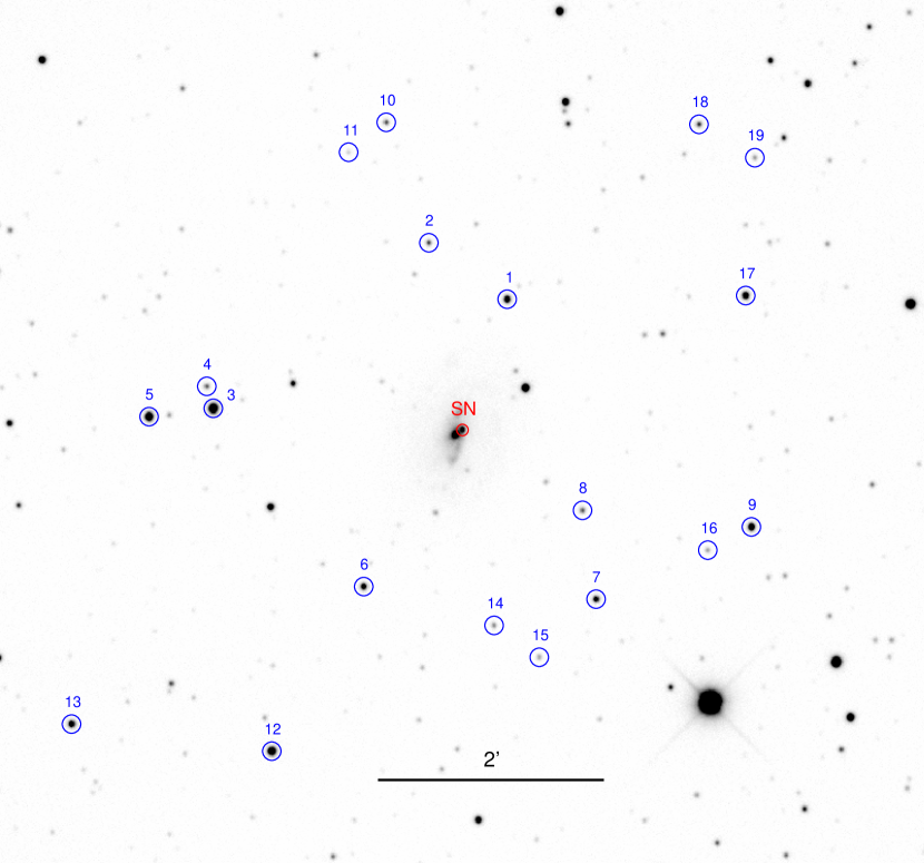
Figure 1.— CHASE $V$-band image of the field of NGC 6000 and SN 2010as. A red circle shows the location of the SN. Numbered blue circles indicate the stars used for photometric calibration (see Tables 1, 2 and 5). The scale of the image is indicated by the horizontal bar. North is up and East is to the left. A close-up of the host galaxy and SN 2010as as observed by VLT with NaCo in the $K$ band can be seen in Figure 13.

2.1. Photometry

Multi-band optical imaging was obtained using the PROMPT $0.41$ m telescopes at CTIO following the SN evolution for over 100 days. Both Johnson-Kron-Cousins $BVRI$ bands and Sloan $g^{\prime}r^{\prime}i^{\prime}z^{\prime}$ bands were used. We observed in $BVRI$ with the PROMPT 1 telescope, in $B$ and $g^{\prime}$ with PROMPT 3, and in $VRI$ and $r^{\prime}i^{\prime}z^{\prime}$ with PROMPT 5. The images covered a field of view of $\approx$ $10^{\prime}\times 10^{\prime}$, with a scale of $0{\farcs}6$ per pixel. Because of lack of accurate guiding of the telescopes, the integration time was set to 40 seconds. Integrations were repeated with each filter in order to obtain high enough signal-to-noise ratios. Each integration was corrected for dark current and flat-fielded before being registered and stacked into a single image per filter.

Because the SN appeared on a bright and complex background, we performed image subtraction in order to obtain accurate photometry. For this purpose we obtained deep reference images in all bands with the PROMPT telescopes between 2011 March and 2012 March, i.e. at least 350 days after the discovery of the SN, and thus when its flux had faded well into the background noise. The subtractions were performed with the hotpants routine.

Photometry of the SN was performed with PSF fitting and calibrated relative to a local sequence of stars in the field of NGC 6000. The field stars are indicated in Figure 1. They were selected to cover a wide range of brightnesses and colors, and to cover the field around the SN while avoiding the bright parts of the host galaxy. The photometric sequence was calibrated to the standard Landolt (Landolt, 1992) and Sloan (Smith et al., 2002) systems using observations from at least two photometric nights (most typically, 3–5 nights). The resulting standard magnitudes of the field stars are listed in Table 1 for $BVRI$, and in Table 2 for $g^{\prime}r^{\prime}i^{\prime}z^{\prime}$. Aparent magnitudes were computed for the SN in the Landolt and Sloan systems, as listed in Tables 3 and 4, respectively. Resulting optical light curves are shown in Figure 2.

Near-infrared (NIR) imaging was obtained in the $JHK$ bands using the Gamma-Ray Burst Optical and Near-Infrared Detector (GROND; Greiner et al., 2008) installed on the MPI $2.2$ m telescope at the La Silla Observatory, Chile. NIR observations started two days after discovery and continued for about 130 days. The field of view covered by the detector was of $10^{\prime}\times 10^{\prime}$, with a pixel scale of $0{\farcs}6$. Reductions were carried out using standard pyraf/IRAF routines to perform dark subtraction, flat-fielding, sky subtraction, image alignment and stacking.

Host-galaxy background flux was subtracted using deep images obtained with GROND on 2011 May 20, that is nearly 430 days after discovery. PSF photometry was performed relative to nine field stars in the Two Micron All Sky Survey (2MASS), which are listed in Table 5. Transformation equations to the standard system were adopted from Greiner et al. (2008). The resulting SN photometry in $JHK$ is listed in Table 6 and plotted in Figure 2.

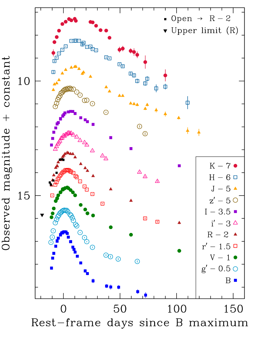
Figure 2.— $BVRIg^{\prime}r^{\prime}i^{\prime}z^{\prime}JHK$ light curves of SN2010as. Black squares correspond to open-filter photometry converted to $R$ band. The black triangle indicates the upper limit of the pre-discovery image, also converted from open filter to the $R$-band scale.

2.2. Spectroscopy

Intensive spectroscopic monitoring of SN 2010as was initiated by the MCSS soon after the discovery, on 2010 March 20 UT, i.e. at $-10.5$ days relative to the time of $B$-band maximum light (see Section 3.1). Seventeen epochs of spectroscopy were obtained, ten of them before maximum light with a nearly nightly cadence. Six post-maximum spectra were obtained on a regular basis for about four months. An additional spectrum was obtained at ten months after maximum.

Most of the spectra covered the optical range and were obtained using long-slit, low-resolution spectrographs. The instruments used were the Wide Field CCD Camera (WFCCD) mounted on the 2.5 m du Pont Telescope at Las Campanas Observatory, the Gemini Multi-Object Spectrograph (GMOS; Hook et al., 2004) on the Gemini South telescope, and the Goodman High Throughput Spectrograph (GHTS; Clemens et al., 2004) on the Southern Astrophysical Research (SOAR) Telescope. The final spectrum was obtained using the Inamori Magellan Areal Camera and Spectrograph (IMACS; Dressler et al., 2011) on the Magellan Baade 6.5 m telescope at Las Campanas Observatory. Medium-resolution, optical and NIR spectroscopy was obtained on four epochs before maximum light using the X-Shooter Spectrograph (Vernet et al., 2011) mounted on the ESO Very Large Telescope (VLT). A log of the spectroscopic observations is given in Table 7.

Reduction of the WFCCD, GHTS and IMACS spectra was performed using standard IRAF routines. Dedicated pipelines were employed for the GMOS and X-Shooter data. When available, spectra of bright featureless stars observed close in time and zenith distance to the SN spectrum were used to correct the telluric absorptions. Flux calibration was performed using standard star spectra observed on each night. The resulting wavelength- and flux-calibrated spectra are shown in the optical range in Figure 3. Figure 4 shows the four spectra from X-Shooter that cover the optical and NIR ranges.

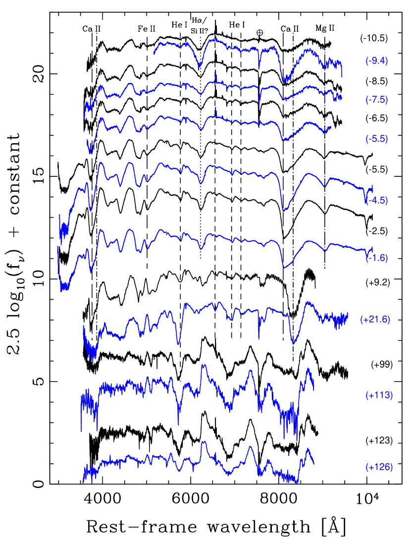
Figure 3.— Optical spectroscopic time-series of SN 2010as between $-11$ and $+126$ days with respect to $B$-band maximum light. The rest-frame epoch of each spectrum relative to $B$-band maximum is indicated in parentheses. Ions responsible for the main spectral features are labeled at the top. Dashed lines show the location of He I lines blueshifted by 5700 km s^-1. The dotted line indicates the location of H$\alpha$ at 15500 km s^-1. Dot-dashed and long-dashed lines show the two components of Ca II lines at 6000 km s^-1 and 14000 km s^-1, respectively. The dot-long-dashed line shows the location of Mg II $\lambda$9227 blueshifted by 6000 km s^-1. The short-long dashed line indicates the location of Fe II $\lambda$5169 at 9500 km s^-1.

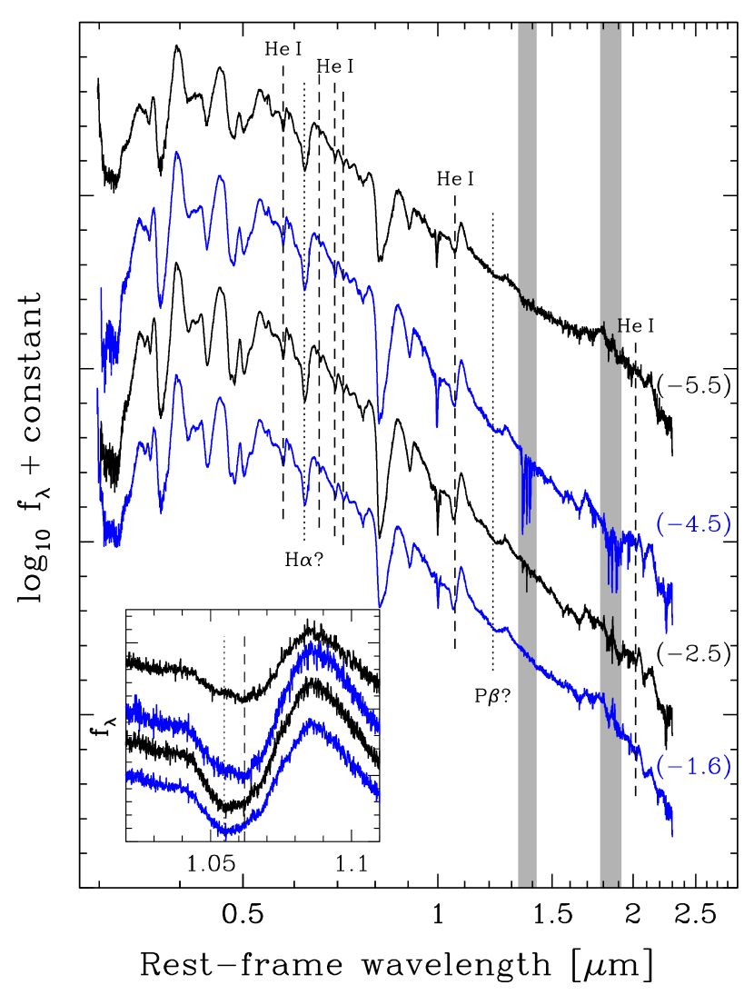
Figure 4.— X-Shooter spectra of SN 2010as obtained between $-5.5$ and $-1.6$ days with respect to $B$-band maximum light. The spectra simultaneously cover the optical and NIR ranges. The numbers in parentheses indicate the epoch of the spectra. Dashed vertical lines show the location of He I lines blueshifted by 5700 km s^-1 while dotted lines indicate the expected location of H$\alpha$ and P$\beta$ at 15500 km s^-1. The gray regions show the wavelength ranges where the atmospheric transmission drops roughly below 50%. The inset shows a zoom around the He I $\lambda$10830 line (note the flux scale is linear). Vertical dashed and dotted lines show the location of the line at 5800 km s^-1 and 7800 km s^-1, respectively.

3. DATA ANALYSIS

3.1. Light Curves

We performed polynomial fits to the light curves of SN 2010as in order to obtain time of maximum light and peak brightness in all bands. In all cases we used polynomials of 3rd or 4th order. To avoid raising the polynomial order and loosing accuracy at maximum light, we only considered data obtained earlier than $\approx$30 days after maximum. The results of the fits are listed in Table 8. In this paper we adopt the time of maximum light in $B$ band, $t_{B}({\mathrm{max}})=2455286.4$ (JD), as the reference epoch. We note an overall drift in the epoch of maximum light toward later times as we move to longer wavelength. This behavior is commonly seen in SE SNe (see, for example, the cases of SN 1999ex and SN 2007Y in Stritzinger et al., 2002, 2009, respectively). The rise and fall timescale of the light curves increases systematically as the effective wavelength increases.

The optical photometry covers from $-11$ days to $\approx$100 days relative to maximum light. The NIR coverage starts two days after and extends until 120 days past maximum. After $\approx$$+70$ days $B$-band and $g^{\prime}$-band coverage stops and the coverage in other optical bands becomes scarce. The NIR light curves continue with good sampling but become noisier after about that epoch due to the increasing relative background level. The $B$ and $g^{\prime}$ light curves show a flattening after about day $+30$, following a steep decline from maximum light. Other bands show a more gradual, linear decline extending until $\approx$$+100$ days.

3.2. Color and Reddening

The location of SN 2010as very near the core of the starburst galaxy NGC 6000 makes this object prone to substantial extinction from dust in the interstellar medium of its host galaxy (see Section 4.1). We thus used the observed SN colors to attempt to determine the amount of reddening and thereby of extinction in any given band. To that end, we first corrected colors by the significant—albeit well-known—Galactic extinction. According to the re-calibrated infrared dust maps of Schlafly & Finkbeiner (2011) the Galactic reddening in the direction of NGC 6000 is $E(B-V)_{\mathrm{Gal}}=0.15$ mag. With this correction applied, we compared the $(B-V)$ color with those of six reddening-free Type Ib and Ic SNe observed by the Carnegie Supernova Project (CSP Hamuy et al., 2006). These reddening-free SNe were selected from the lack of narrow Na I D absorptions in the spectra, and by being relatively away from star-forming regions in their host galaxies. They were used to calculate an average intrinsic $(B-V)$ color curve between the time of $B$-band maximum light and 20 days after, which is shown in the upper-left panel of Figure 5 (Stritzinger et al., in preparation). The color curve evolves monotonically from $(B-V)=0.35$ mag to $(B-V)=1.08$ mag in such epoch range, with a typical dispersion of $0.06$–$0.14$ mag. SN 2010as exhibits a similar trend in the $(B-V)$ color evolution but with systematically redder observed colors. By assuming the deviation is due to reddening in the host galaxy, we derived $E(B-V)_{\mathrm{Host}}=0.42\pm 0.02$ mag from the weighted average of the deviations. A systematic uncertainty of $\approx$$0.1$ mag can be added to this due to the dispersion in the intrinsic colors.

We also compared our $(V-R)$ colors with the average intrinsic colors for Type Ib and Ic SNe derived by Drout et al. (2011). These averages are taken at 10 days past the time of maximum in $V$ and in $R$ bands, with $\langle(V-R)\rangle_{V10}=0.26\pm 0.06$ mag and $\langle(V-R)\rangle_{R10}=0.29\pm 0.08$ mag, respectively. After correcting for Galactic extinction, we obtain $(V-R)_{V10}=0.62\pm 0.2$ mag and $(V-R)_{R10}=0.65\pm 0.2$ mag for SN 2010as. Averaging the differences with both reference values, we obtain $E(V-R)_{\mathrm{Host}}=0.36\pm 0.05$ mag. If we assume a standard reddening law from Cardelli et al. (1989) with total-to-selective absorption coefficient $R_{V}=3.1$, this can be converted to $E(B-V)_{\mathrm{Host}}=0.67\pm 0.09$ mag. This value is in disagreement—although at a $1.8$-$\sigma$ level—with that obtained from the comparison of $(B-V)$ colors of the CSP sample. The discrepancy may be due to the fact that Drout et al. (2011) derived their intrinsic colors using a sample of ten SE SNe from the literature, including Type Ib, Ic, IIb and three Ic-BL objects. The photometric systems and estimated extinctions affecting those SNe are thus of very diverse origin. Our comparison of $(B-V)$ colors with those in the CSP sample is probably more robust. Also, we consider this higher reddening to be unrealistic because it would produce too blue colors in other bands, as shown below.

We further estimated reddening from the Balmer decrement based on the narrow emission-line flux ratio of H$\alpha$ to H$\beta$. This was done on spectra extracted nearby the SN location and adopting case B recombination with $n_{e}\sim 10^{2}$–$10^{4}$ cm^-3 and $T_{e}=10^{4}$ K (Osterbrock, 1989). From this we obtained a value of $E(B-V)_{\mathrm{Host}}=0.44$ mag, in agreement with the value from the $(B-V)$ color. In addition, we could clearly detect three sets of Na I D absorption lines in the spectra at all phases. One component appeared at rest, in agreement with the existence of Milky-Way gas and dust in the line of sight, and the other two components appeared with recession velocities of about 2020 and 2240 km s^-1, i.e. at $\approx$$-170$ and $\approx$50 km s^-1 with respect to the systemic recession velocity of the host galaxy. We measured the equivalent widths (EW) of the Na I D doublet and found no evidence of variation with phase. The average EW was of $0.7$ Å for the Galactic component, and $2.1$ Å and $0.5$ Å for the two components in NGC 6000. Although the EW of Na I D does not provide an accurate estimate of the color excess (Phillips et al., 2013), the relative strength of the absorptions is in agreement with the presence of higher extinction in the host galaxy, as compared with that in the Milky Way.

Based on the analysis above, we adopted $E(B-V)_{\mathrm{Host}}=0.42\pm 0.1$ mag to compute the reddening-corrected colors. Selected color indices are shown in Figures 5 and 6 in comparison with intrinsic colors for a sample of well-observed SE SNe. For the comparison SNe, colors were corrected for Galactic and host-galaxy reddening by adopting color-excess values from the literature and a standard reddening law with $R_{V}=3.1$. As expected, the corrected $(B-V)$ colors of SN 2010as (upper-left panel of Figure 5) agree well with most SE SNe. However, using $R_{V}=3.1$ for the host-galaxy reddening of SN 2010as, its other colors, especially those involving a wide wavelength span, appeared too blue in comparison with the rest of the objects. For example, SN 2010as would be intrinsically bluer than all other SE SNe near maximum light by $\approx$$0.2$ mag in $(V-I)$ and $(r^{\prime}-i^{\prime})$, by $\approx$$0.4$ mag in $(V-J)$, and by $\approx$$0.6$ mag in $(V-H)$. We attributed this behavior to the adopted value of $R_{V}$ for the host-galaxy reddening. By lowering it to $R_{V}=1.5$, as shown in the figures, we obtained a much better agreement with the comparison sample, consistently for all the colors. Similarly low values of $R_{V}$ have typically been found for Type Ia SNe with significant reddening (see Phillips et al., 2013), and in studies of Type II-Plateau SNe (Olivares et al., 2010). The origin of low $R_{V}$ values may be linked to the properties of the dust grains, or to the presence of a dense circumstellar shell of dust around the SN. In Section 3.3 we present further support for a low $R_{V}$ from our calculation of the bolometric luminosity. We thus adopted a non-standard, low, reddening law parameter of $R_{V}=1.5$ for SN 2010as. Due to the observed dispersion of colors among SE SNe, which is significantly larger than that found among Type Ia SNe, a precise derivation of $R_{V}$ is not possible. In the future, such a study may be addressed provided there is a consistent photometric dataset for a homogeneous SN sample.

From Figures 5 and 6 we see that there is a group of SE SNe that agree in their color evolution, especially from a few days before maximum and on. In the optical regime colors tend to agree better whereas when near-infrared bands are involved (see Figure 6) the dispersion becomes large, e.g., as much as 1 mag in $(V-J)$ and $(V-H)$. The outlying object in this sample is the peculiar SN 2005bf that showed doubly peaked light curves and very large luminosity (Anupama et al., 2005; Tominaga et al., 2005; Folatelli et al., 2006). Its colors are consistent with most SE SNe near maximum light, but as the SN evolved to its second peak, optical colors became blue again and remained so for about 40 days, drastically deviating from the rest of the SNe.

We computed reddening-free peak absolute magnitudes in all observed bands using the reddening estimate derived above and the distance to the host galaxy of $27.38\pm 4.74$ Mpc (distance modulus of $\mu=32.16\pm 0.36$ mag) from the NASA/IPAC Extragalactic Database (NED). This distance is an average of six measurements based on the Tully-Fisher method from the Nearby Galaxy Catalog (Tully, R. B. 1988), and later by Terry et al. (2002); Theureau et al. (2007). The resulting absolute magnitudes are listed in Table 8.

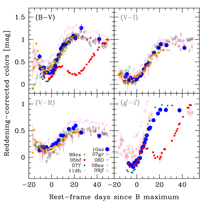
Figure 5.— Color curves of SN 2010as (black dots) compared with other SE SNe. Colors were corrected for total reddening (see text for details). The solid curve in the upper-left panel shows the locus of the intrinsic $(B-V)$ colors of SE SNe as derived from the CSP sample (Stritzinger et al., in preparation), with dotted lines indicating the 1-$\sigma$ dispersion. Comparison SE SNe from the literature comprise the Type IIb SN 2008ax (Pastorello et al., 2008) and 2011dh (Ergon et al., 2014), the Type Ib SN 2008D (Modjaz et al., 2009) and SN 2009jf (Valenti et al., 2011; Sahu et al., 2011), the Type Ic SN 2007gr (Valenti et al., 2008; Hunter et al., 2009), and finally the transitional Type Ib/c SN 1999ex (Stritzinger et al., 2002), SN 2005bf (Folatelli et al., 2006) and SN 2007Y (Stritzinger et al., 2009).

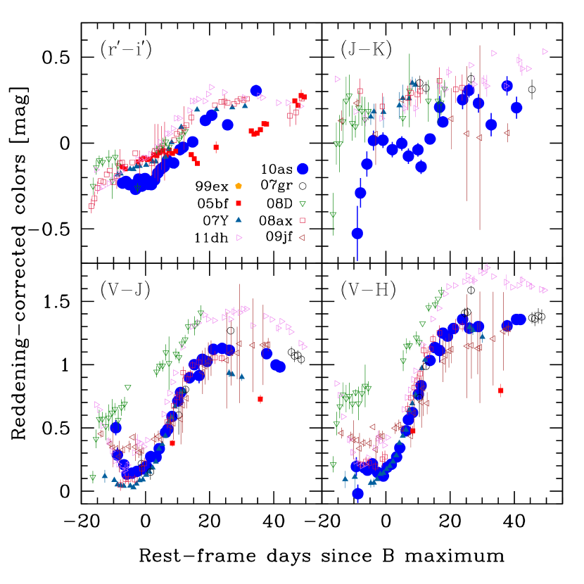
Figure 6.— Color curves of SN 2010as (black dots) compared with other SE SNe. Colors were corrected for total reddening (see text for details). See references of data sources in Figure 5.

3.3. Bolometric Luminosity

We used the broad-band photometry to compute the integrated flux, $F_{B\rightarrow K}$, in the range between $B$ and $K$ bands. For this purpose, we converted observed magnitudes, corrected by extinction as in Section 3.2, to monochromatic fluxes at the effective wavelength of each filter. The conversions of magnitude to flux were performed using the spectral energy distribution of Vega as given by Bohlin & Gilliland (2004a). When an observation in a given band was missing, we used a low-order interpolation of the neighboring observations in that band. Monochromatic fluxes at a given date were then trapezium-integrated in wavelength to produce the pseudo-bolometric flux $F_{B\rightarrow K}$.

In order to account for the missing flux outside the wavelength range covered by our photometry, we used extrapolations. On the UV regime we assumed that the flux dropped linearly from the value measured at the effective wavelength of the $B$ band (at 447 nm) to zero flux at 200 nm and that the flux blueward of that wavelength was negligible (Bersten& Hamuy, 2009; Lyman et al., 2014). This assumption is based on observations of core-collapse SNe (Panagia, 2003; Bufano et al., 2009). We simply integrate the flux in such triangle to obtain the UV contribution, $F_{\mathrm{UV}}$. The flux redward of the $K$ band, $F_{\mathrm{IR}}$, was estimated by extrapolating a black-body (BB) fit of the observed monochromatic fluxes. Table 9 provides the fitted BB radii, $R_{\mathrm{BB}}$, and temperatures, $T_{\mathrm{BB}}$. If the fitted BB temperature was high enough, the Rayleigh-Jeans (R-J) approximation was adopted. Otherwise, the BB was integrated between the effective wavelength of the $K$ band and 15000 nm, which produces a good approximation of the integration until infinite wavelength. The total bolometric flux was thus computed as $F_{\mathrm{Bol}}=F_{B\rightarrow K}+F_{\mathrm{UV}}+F_{\mathrm{IR}}$. Figure 7 shows the percentage contribution of $F_{B\rightarrow K}$, $F_{\mathrm{UV}}$, and $F_{\mathrm{IR}}$ with time, along with the evolution of the BB temperature and radius, and the reddening-free $(B-V)$ color. Due to the long wavelength coverage of the data, the estimated contribution of the extrapolated fluxes is moderate at all times. The actually measured flux, $F_{B\rightarrow K}$, is always greater than 70 percent of the total flux. As shown in Figure 7, before maximum light the ejecta are hot and the UV contribution is relatively important. Nevertheless it is always below 30%. The IR contribution is small at all times and remains below 6% during the time considered here. In Figure 7 we also show the BB temperature evolution when assuming a host-galaxy reddening law with $R_{V}=3.1$. Initially, the resulting temperatures are unrealistically high. This is an additional indication of a low $R_{V}$, as derived in Section 3.2.

Bolometric fluxes were converted to luminosities adopting a distance of $27.38\pm 4.74$ Mpc from NED. Table 9 lists the luminosity integrated between $B$ and $K$ ($L_{B\rightarrow K}$) and the estimated bolometric luminosity ($L_{\mathrm{Bol}}$). In Table 8 we included the peak apparent and absolute bolometric magnitudes obtained from a polynomial fit to the bolometric light curve. The bolometric light curve is shown in Figure 8 along with several well-studied SE SNe. For comparison, we also show $L_{B\rightarrow K}$ computed as described above, and the resulting $L_{\mathrm{Bol}}$ for zero host-galaxy reddening, and for $E(B-V)_{\mathrm{host}}=0.42$ mag with $R_{V}=3.1$ (dashed and dotted lines, respectively). For SNe 2005bf and 2008D we obtained the bolometric luminosities directly from the literature because they were computed in a similar fashion as that described here. For the rest of the objects we calculated bolometric luminosities using the color-based bolometric corrections provided in Table 2 of Lyman et al. (2014). All available colors were employed for each SN, and the resulting luminosities were averaged. Estimates of Galactic extinction and distances were obtained from NED. Host-galaxy extinction values were adopted from the literature.

The peak bolometric luminosity of SN 2010as occurred about $1.5$ days after the peak in the $B$ band, with a value of $(2.7\pm 1.0)\times 10^{42}$ erg s^-1. The uncertainty in the luminosity was estimated by considering uncertainties in distance, extinction and the estimated error in the extrapolations done to compute $F_{\mathrm{UV}}$, and $F_{\mathrm{IR}}$. The uncertainty in distance implies a 34% uncertainty in luminosity. This is the dominant component, and is constant in time. From the $0.1$ mag uncertainty in $E(B-V)$, we derived an uncertainty of $\approx$10% in luminosity. We assumed the extrapolations to contain a 20% uncertainty, which corresponds to 6% of the total flux. Assuming the explosion happened at the midpoint between the last non-detection and the discovery, the rise time to maximum luminosity was of $16.5\pm 3$ days. The bolometric light curve of SN 2010as is similar to that of SN 1999ex. The first peak of SN 2005bf also shows a similar evolution, before it re-brightens to a wide and luminous main peak. The Type IIb SNe 2008ax and 2011dh show similar light-curve shapes with slightly slower rise and lower peak luminosity. The Type Ib objects shown here (SNe 2008D and 2009jf) have wide bolometric light curves—with an initial decline in the case of SN 2008D.

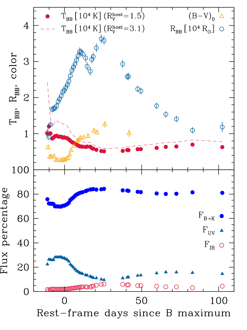
Figure 7.— Top: Evolution of the fitted BB temperature (filled circles) and radius (open circles), and of the intrinsic $(B-V)$ color (triangles), as a function of the rest-frame time since maximum bolometric luminosity. Bottom: Estimated contributions to the total flux outside the observed wavelength range. $F_{\mathrm{UV}}$ is the estimated flux blueward of the $B$ band, and $F_{\mathrm{IR}}$ is the estimated flux redward of the $K$ band (see text for details).

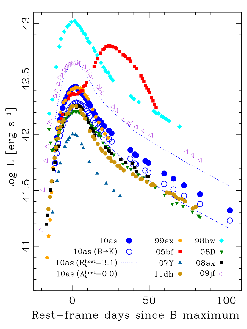
Figure 8.— Bolometric light curve of SN 2010as compared with SE SNe from the literature (see references in the text). Filled blue circles show the estimated bolometric luminosity of SN 2010as, after correcting for total extinction, with $R_{V}=1.5$ for the host-galaxy extinction. Open blue circles show the contribution that was actually observed, integrated between the $B$ and $K$ bands. The dotted curve indicate the bolometric luminosity that would result by assuming $R_{V}=3.1$ for the host-galaxy reddening. The dashed curve shows the case of no extragalactic extinction. Comparison SNe are: the transitional Type Ib/c SN 1999ex (Stritzinger et al., 2002), SN 2005bf (Folatelli et al., 2006), and SN 2007Y (Stritzinger et al., 2009); the Type Ib SN 2008D (Modjaz et al., 2009) and SN 2009jf (Sahu et al., 2011; Valenti et al., 2011); the Type IIb SN 2008ax (Pastorello et al., 2008; Taubenberger et al., 2011) and SN 2011dh (Ergon et al., 2014); and the broad-line Type Ic SN 1998bw (Clocchiatti et al., 2011).

3.4. Spectroscopic Properties

The spectroscopic follow-up of SN 2010as continued between $-11$ and $+309$ days relative to $B$-band maximum light, with nearly daily coverage before maximum. This allowed us to perform a detailed study of the evolution of spectral properties for this object.

3.4.1 Photospheric Phase

We study here the spectra obtained between $-11$ and $+22$ days relative to $B$-band maximum light, when a clear continuum emission could be identified. As seen in Figure 3, the first spectrum has mostly Type Ic characteristics. It is dominated by wide Ca II and Fe II absorption features with very slight signs of He I lines. Helium lines slowly increase in strength with time and become conspicuous in the optical range not earlier than a few days before maximum. He I $\lambda$10830 is clearly identifiable in our pre-maximum NIR spectra (Figure 4), as is expected since this is usually the strongest helium feature. Ca II and Fe II absorptions remain strong throughout the epoch range sampled here. In particular, Ca II lines evolve from being dominated by large Doppler-shift components before maximum, to much lower shifts after maximum. A strong absorption at about 6200 Å is also present at least until maximum light. Such feature has been observed in other Type Ib and Ic objects and its identification is unclear (Branch et al., 2006; Elmhamdi et al., 2006; Ketchum et al., 2008; Spencer & Baron, 2010). Here we will evaluate the most probable associations, which are Si II $\lambda$6355 or H$\alpha$. The identification of this feature is crucial for the understanding of the nature of SN 2010as in the context of SE SNe.

In order to provide a more secure identification of the elements present in the ejecta and their approximate distribution, we performed synthetic spectrum calculations using the SYNOW code (see Branch et al., 2002, and references therein). Figure 9 shows SYNOW calculations compared with spectra observed at three different epochs. In this simple model, the continuum emission is assumed to be due to a black body of given temperature, $T_{\mathrm{BB}}$, defined at a sharp photosphere. The ejecta distribution is given in velocity space, which can be interpreted as a spatial coordinate by assuming homologous expansion. Line profiles are computed in the Sobolev approximation by arbitrarily fixing a distribution of optical depth ($\tau$) as a function of velocity for each ionic species. The photospheric velocity, $v_{\mathrm{ph}}$, thus fixes the minimum shift of absorption lines in the spectrum. Relative line strengths for each species are determined by fixing its excitation temperature, $T_{\mathrm{exc}}$, and assuming local thermal equilibrium. Here we adopted consistent $T_{\mathrm{exc}}$ of 8000–10000 K for all species, except for H I as explained below. Considering the simplifications of the model, the synthetic spectra agree quite well with the observations.

The main species included in the synthetic spectra were He I, O I, Mg II, Ca II, Ti II and Fe II. Additional presence of Na I is probable after maximum light. The inclusion of H I or Si II will be discussed below. In order to reproduce the small blueshift of most observed lines, we needed to set low values of $v_{\mathrm{ph}}$ even at the earliest phases. For the first spectrum at $-10.5$ days we adopted $v_{\mathrm{ph}}=6000$ km s^-1, and this value remained nearly unchanged until nine days after maximum light. Only after that time did the photospheric velocity decrease to $\approx$4000 km s^-1 at $+22$ days, and $\approx$3500 km s^-1 at about $+100$ days. For all the elements listed above the line-forming region was consistent with being attached to the photosphere. Even at such low velocities, the line profiles appeared broad, which required a shallow dependence of the optical depth as a function of velocity. For all the species we adopted a power law for $\tau\propto v^{-\alpha}$, with $\alpha$ being 3 until maximum light and 4 or 5 after maximum. The assumed maximum optical depths of all elements grew consistently until nine days after maximum light.

The large blue extent of the Ca II absorptions and the shape of the Fe II complex at $\approx$5000 Å required extra components at high velocity. The calcium and iron line profiles were best reproduced by assuming an additional shell with a Gaussian optical-depth distribution. The central velocity of the shells decreased with time from 11000 km s^-1 at $-10.5$ days to 7000 km s^-1 and 10000 km s^-1 at maximum light for Ca II and Fe II, respectively. The Ca II shell had a Gaussian width of $\sigma_{v}=5000$–6000 km s^-1, while a narrower Fe II shell of $\sigma_{v}=2000$ km s^-1 was invoked. Both high-velocity components had disappeared by nine days after maximum.

The strong absorption at 6200 Å was not accounted for by any of the species described above. We studied whether it was reproduced by Si II $\lambda$6355 forming near the photosphere, by high-velocity (detached) H$\alpha$, or by a combination of both. As shown in Figure 9, both the synthetic Si II and H$\alpha$ lines provide reasonable approximations to the observations before and at maximum light. Other lines of the same species are too weak to be distinguished, as indicated by the fact that both synthetic spectra are identical. An exception to this may be P$\alpha$ which, depending on the adopted excitation temperature, can become quite strong in the SYNOW spectrum. However, by adopting $T_{\mathrm{exc}}\approx 5000$ K, the strength of P$\alpha$ could be reduced to match the observation, as shown in the upper inset of Figure 9. We note that P$\alpha$ may be partly affected by atmospheric absorption. While P$\beta$ is not noticeable in the synthetic spectrum, the data show an absorption matching this line blueshifted by the same velocity as H$\alpha$. This line is present in all four of our NIR spectra (see Figure 4). Moreover, the presence of hydrogen is further supported by the spectrum at $+9$ days (see lower inset in Figure 9). In that spectrum the Si II $\lambda$6355 line fails to reproduce the location of the observed absorption that is still identifiable among Fe II lines. Instead, H$\alpha$ shifted by about 10000 km s^-1 produces a good agreement with the observation. We can conclude from the SYNOW analysis that SN 2010as showed at least a small amount of hydrogen present at high velocity.

As we noted above from the SYNOW calculations, SN 2010as showed quite low expansion velocities even at the earliest time. Moreover, the photospheric velocity remained nearly constant between $-11$ and $+9$ days. We studied this behavior in greater detail by looking at the expansion velocities measured from the shifts of the absorption minimum of the lines. Such velocities are shown in Figure 10 for He I, Mg II, Ca II and Fe II lines. The case of H$\alpha$ is also shown. Before maximum light, the lowest velocities correspond to He I lines at $\approx$5500 km s^-1, followed closely by Mg II. The velocity of He I $\lambda$10830 shows a rapid increase during the interval sampled by the NIR observations. The inset of Figure 4 shows that this line appears as a double absorption with components at $\approx$5800 km s^-1 and $\approx$7800 km s^-1, if both are attributed to He I. The measured velocity increases as the blue component begins to dominate over the red one. It can also be that the He I line produces the red component at a constant velocity of $\approx$5800 km s^-1, while the other absorption is due to C I $\lambda$10693, although in that case the carbon velocity would be too low ($\approx$4000 km s^-1), and no other carbon lines are apparent in the spectra. Our SYNOW analysis shows that the low expansion velocities is not a peculiarity of the helium lines, but rather a property of the photosphere.

High-velocity components of Fe II and Ca II dominate before maximum, and so the measured velocities for these species are significantly larger than the photospheric one. Fe II $\lambda$5169 appears blueshifted at $\approx$9000 km s^-1. This is a consequence of the blend of low- and high-velocity components mentioned in our SYNOW analysis. Ca II lines and H$\alpha$ appear at 14000–17000 km s^-1. At nine days after maximum, all species show similar, low velocities around 6000 km s^-1, including Fe II and Ca II, whose high-velocity components disappear. By day $+22$ we notice a larger dispersion of line velocities, with Fe II showing the lowest value. At this phase the He I $\lambda$5876 and $\lambda$7065 lines have velocities that differ by over 2000 km s^-1. This may be due to the presence of Na I blended with He I $\lambda$5876, as suggested by the SYNOW calculation for this epoch.

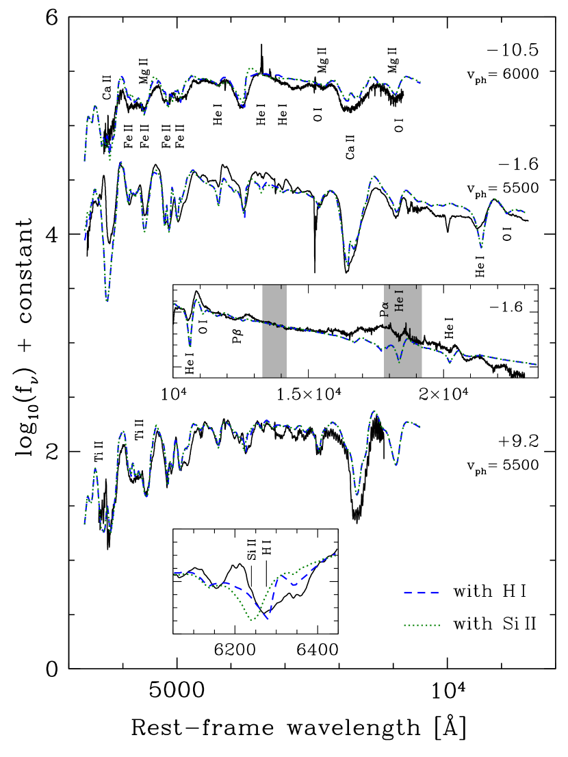
Figure 9.— Synthetic spectra computed with SYNOW compared with the spectra of SN 2010as obtained at $-10.5$, $-1.6$ and $+9.2$ days (solid black lines). The SYNOW spectra including H I at high velocity are shown with dashed blue lines. Alternative calculations without hydrogen and with Si II are shown with dotted green lines. The main ions that contribute to the observed features are indicated. The top inset graph shows the NIR range of the spectrum from $-1.6$ days. The bottom inset panel shows the detail around the H$\alpha$ line at $+9.2$ days where we indicated the location of the Si II $\lambda$6355 line at photospheric velocity, and the H$\alpha$ line detached at about 10000 km s^-1.

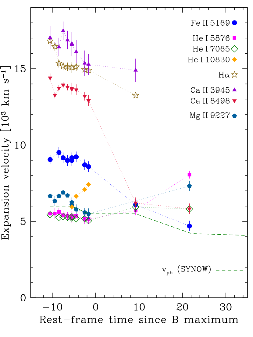
Figure 10.— Expansion velocities of SN 2010as as measured from the blueshift of the maximum absorption on well-identified lines. The dashed curve shows the photospheric velocity adopted in the SYNOW models.

3.4.2 Transitional and Nebular Phases

Several spectra obtained between $+98$ and $+126$ days show the transition to the nebular phase (see Figure 3), when the continuum level decreases and emission lines begin to dominate. At this stage the most prominent spectral features are due to oxygen and calcium. O I $\lambda$7774 and the Ca II infrared triplet are seen predominantly in emission. Our last spectrum obtained at $+309$ days is well in the nebular phase. It is shown in Figure 11 in comparison with those of other SE SNe. At this stage the density has decreased enough for forbidden lines to dominate. The most prominent of those lines are the doublets of [O I] $\lambda\lambda$6300, 6363 and [Ca II] $\lambda\lambda$7291, 7324. Apart from them, only Mg I$]$ $\lambda$4571 and possibly very weak Na I D and Ca II infrared triplet can be seen at this late time.

During the transitional phase, about 100 days after maximum, a bump is observed on the red wing of the [O I] $\lambda\lambda$6300, 6363 emission. This can be seen in Figure 3, around the narrow H$\alpha$ and [N II] lines produced by an underlying H II region. Such feature has been observed in Type IIb SNe and in some Type Ib objects and has been attributed to H$\alpha$. Such emission is clearly visible in SNe 2005bf and 2007Y (see Figure 11). In the case of SN 2010as we observe that around $+100$ days its profile is complex, which may indicate the presence of other lines. The emission may still be present in the spectrum obtained at $+309$ days, although the data are very noisy. We thus cannot provide further evidence of the presence of hydrogen from the nebular spectra.

In Figure 12 we show the evolution of [O I] $\lambda\lambda$6300, 6363, [Ca II] $\lambda\lambda$7291, 7324, and O I $\lambda$7774 during the transition to the nebular phase. The strength of both the permitted and forbidden O I lines decrease substantially at $+309$ days while the [Ca II] feature remains nearly constant. The [O I] feature presents a double peak with a central trough that appears slightly blueshifted relative to the adopted reference wavelength of 6300 Å. The other two features show singly-peaked profiles, possibly with a central cusp in the case of [Ca II]. Such doubly-peaked [O I] profiles have been observed in other SNe (Mazzali et al., 2005; Maeda et al., 2008; Modjaz et al., 2008; Taubenberger et al., 2009) and their nature is under debate. While Maeda et al. (2008) proposed that the shape is due to an asymmetric distribution of the inner oxygen-rich material, Milisavljevic et al. (2010) suggest that at least in some SNe a geometrical explanation is not necessary because we are simply observing the two lines of the doublet. The latter scenario, however, has problems in explaining deviations from the 3:1 flux ratio expected between the $\lambda$6300 and $\lambda$6363 lines, and the fact that a significant fraction of objects show a singly peaked [O I] profile (Maeda et al., 2008; Taubenberger et al., 2009). Finally, Maurer et al. (2010) suggest that the central trough may be due to high-velocity H$\alpha$ absorption. In this case, the velocity of H$\alpha$ would be 13000 km s^-1, which is compatible with the velocity measured nine days after maximum light (see Figure 10).

Assuming we are observing two components of the [O I] doublet, Figure 12 shows a blueshifted and a redshifted peak, which is in general agreement with the picture of an edge-on disk or torus of O-rich material. The trough between the peaks appears slightly blueshifted, which may be due to self-absorption in the torus/disk structure that blocks part of the emission from the receding sector that is farthest from the observer. We note that the blueshift of the central trough decreases from $\approx$600 km s^-1 at about 100 days to $\approx$200 km s^-1 at $+309$ days. This observation is consistent with a reduction in the internal opacity as the ejecta expands. Interestingly, during this period the [Ca II] $\lambda\lambda$7291, 7324 feature appears redshifted from the adopted reference wavelength of $7307.5$ Å. The amount of redshift also decreases with time, from $\approx$2000 km s^-1 to $\approx$900 km s^-1. This seems to be a peculiar feature of SN 2010as, as in general the [Ca II] emission appears at rest or slightly blueshifted in other well-observed SNe. The origin of the redshift may be an asymmetric distribution of the inner calcium-rich material, or a large degree of contamination of this feature by lines emitted redward of the central [Ca II] wavelength. If such contamination were due to [Fe II], the lines around this [Ca II] feature would likely be stronger on the blue side ($\lambda\lambda$7155, 7172) than on the red side ($\lambda\lambda$7388, 7452; Garstang, 1962), and thus it would not produce a net redshift. Although very noisy, the Mg I$]$ $\lambda$4571 line observed at $+309$ days also appears redshifted by about 1400 km s^-1, which provides support to the peculiar redshift of the [Ca II] doublet.

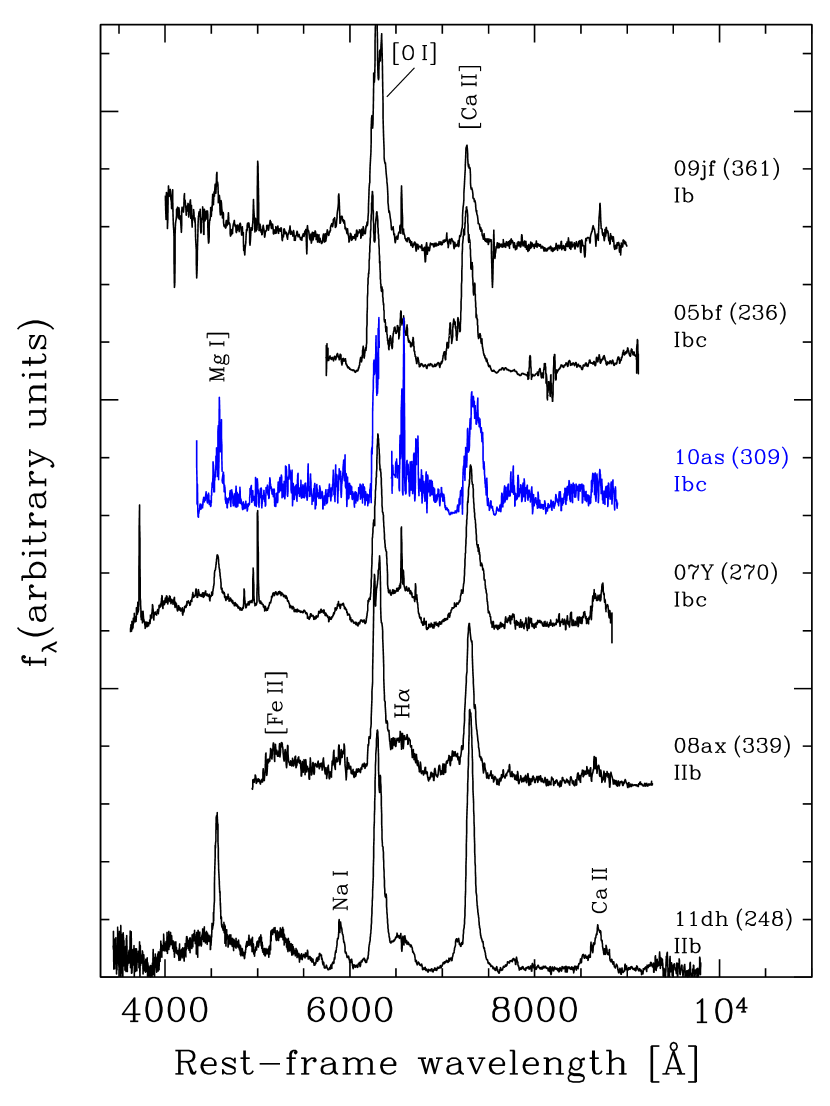
Figure 11.— Nebular spectrum of SN 2010as compared with those of other SE SNe at similar epochs (given in parentheses with respect to $B$-band maximum light). Ions for the main observed features are indicated. H$\alpha$ can be seen as a bump on the red side of the [O I] $\lambda$$\lambda$6300,6363 emission, except for the Type Ib SN 2009jf. For SN 2010as, the cut in the wavelength coverage and the noise in the data make the identification of H$\alpha$ difficult.

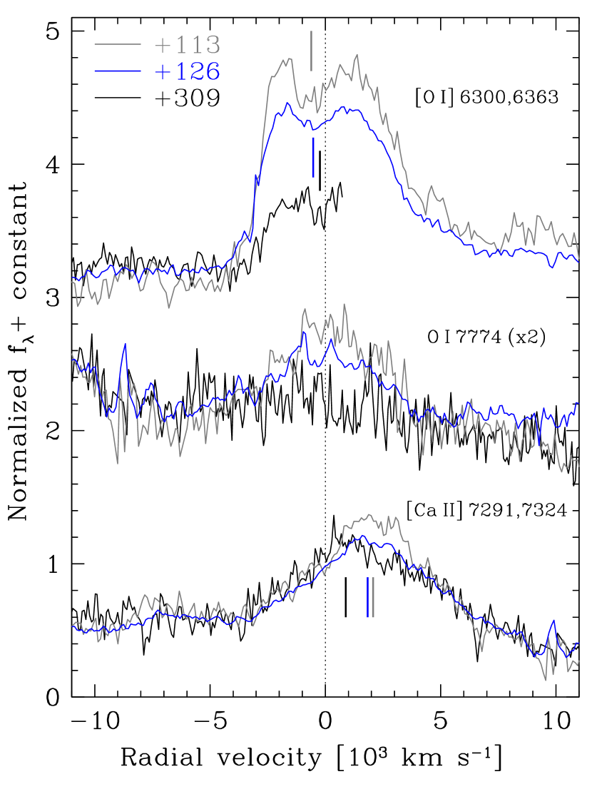
Figure 12.— The main emission lines observed in the transitional and nebular spectra of SN 2010as, plotted in velocity space. The spectra are from $+113$ days (gray), $+126$ days (blue), and $+309$ days (back). Reference wavelengths were assumed as 6300 Å for the [O I] $\lambda$$\lambda$6300,6363 doublet, 7774 Å for O I $\lambda$7774, and 7307.5 Å for [Ca II] $\lambda$$\lambda$7291,7324.

4. ENVIRONMENT AND PROGENITOR OF SN 2010as

4.1. Host Galaxy and Environment

SN 2010as appeared very near the nucleus of the starburst galaxy NGC 6000, of morphological type “SB(s)bc:” (RC3; De Vaucouleurs et al., 1991). NGC 6000 has been cataloged as a luminous infrared galaxy (LIRG; Sanders et al., 2003) and it is also luminous in the optical and the NIR ranges. It has been reported as an active galaxy with nuclear a H II region (Moran et al., 1996). By modeling mid-infrared observations, Siebenmorgen et al. (1999) and Siebenmorgen et al. (2004) concluded that large amounts of dust are present in the nuclear region of the galaxy, with a central extinction between $A_{V}=20$ and $A_{V}=29$ mag. Adopting a distance of $27.38\pm 4.74$ Mpc (NED), the SN location is at a projected distance of only $490\pm 23$ pc from the galaxy center. We therefore expect the SN to be located in a region of rich star formation, with enriched gas and probably large amounts of dust. Details about the underlying stellar population at the specific location of the SN were obtained from the HST pre-SN images and are described in Section 4.2.

We studied the abundance of metals in the vicinity of the SN and in the galaxy as a whole. For that purpose, we used the deep spectrum obtained when the SN was 309 days after maximum to extract spectra of the host-galaxy light at different locations along the slit. We detected narrow emission lines from H II regions at different angular distances from the SN. The extraction at the closest proximity to the SN was done at a distance of $2{\farcs}2$, which means a projected distance of 290 pc. We used the calibrations of Pettini & Pagel (2004) to determine oxygen abundances based on flux ratios. Adopting the $O3N2$ calibration, our measurements nearest the SN resulted in $\log(\mathrm{O/H})+12=8.80$. If we adopt a solar metallicity ($Z_{\odot}$) of $\log(\mathrm{O/H})+12=8.69\pm 0.05$ (Asplund et al., 2009), the environment of SN 2010as has a metallicity of $1.3\,Z_{\odot}$. The $N2$ index of Pettini & Pagel (2004) is not well-suited for this SN because the measured line ratio is near the extreme of the relation. However, by adopting both linear and cubic relations (their equations 1 and 2), we obtained $\log(\mathrm{O/H})+12=8.75$ and $8.95$, which corresponds to $1.1$ $Z_{\odot}$ and $1.8$ $Z_{\odot}$ respectively. This suggests that the environment has super-solar metallicity. Near the SN location, the measurement may be affected by the proximity of the galaxy nucleus. We therefore performed the same measurement at longer distances and found values of $\log(\mathrm{O/H})+12=8.74$ at projected distances of up to 5 kpc from the nucleus. This provides further evidence for the super-solar metallicity in the environment of SN 2010as.

4.2. Pre-Explosion Observations

The field of SN 2010as was observed by the HST before the explosion of the SN. Two images of NGC 6000 were retrieved from the Hubble Legacy Archive. The images were obtained with the Wide Field Planetary Camera 2 (WFPC2) on 1996 February 19, using the F606W filter (PI: Stiavelli) with a total exposure time of 600 seconds. Additional observations were found for a total exposure of 384 seconds in the F160W filter, obtained using the Near Infrared Camera and Multi-Object Spectrometer (NICMOS) on 1997 July 5. We used these observations to study the nature of any possible source in the pre-explosion images that could be associated with the progenitor of SN 2010as.

In order to accurately determine the position of the SN in the WFPC2 images, we used high-resolution, adaptive optics observations obtained in the $K_{s}$ band using the NAOS-CONICA (NaCo) instrument (Lenzen et al., 2003; Rousset et al., 2003) at the Very Large Telescope of ESO by PI Smartt on 2010 March 27, i.e., a few days before the SN reached maximum light. Forty-eight dithered images of 60 seconds each were processed and combined using the dedicated NaCo pipeline provided by ESO. We used IRAF routines in order to locate common objects in the NaCo and WFPC2 F606W image and to calculate the coordinate transformation. With five objects in common, we obtained a coordinate match with a precision of 16 mas, considering the uncertainty in the plate solutions for both NaCo and WFPC2 images (2 mas and 14 mas, respectively), and the geometric transformation uncertainty of 6 mas, added in quadrature. The SN coordinates in the NaCo image resulted as $\alpha=15^{\mathrm{h}}49^{\mathrm{m}}49{\fs}228$, $\delta=-29^{\circ}23^{\prime}09{\farcs}72$, in good agreement with previous determinations.

Using the above registration, we were able to identify a source that was coincident with the SN location in both WFPC2 and NICMOS images, as shown in Figure 13. The WFPC2 image shows that there were actually three objects in the vicinity of the SN location. The brightest source (S1) is also the closest one to the SN location, at a distance of $0{\farcs}04$—i.e., less than one pixel away, and less than 5 pc away in projected distance. We indicate the other two sources with S2 and S3 in order of decreasing F606W brightness. S2 is located at $2.2$ pixels to the southeast of S1, that is at a projected distance of $\approx$13 pc. S3 is located at $3.5$ pixels to the NW of S1, with a projected distance of $\approx$21 pc. S1 appears to have a slightly extended profile with FWHM of $1.9$ pixels—to be compared with the point-source FWHM of $1.3$ pixels for this instrument (Krist et al., 2011). In the F160W images only one source is visible. This may be due to the coarser resolution of the NICMOS image (the PC chip of WFPC2 has a plate scale of $0{\farcs}046$ per pixel, whereas the scale of NICMOS is $0{\farcs}075$ per pixel). Indeed, the FWHM of the source is of $2.4$ pixels in the NICMOS image, and S2 and S3 would be located at $1.4$ and $2.2$ pixels from S1, respectively. We thus identify the source in the NICMOS image with S1, although it may include flux from the unresolved S2 and S3 sources.

We performed PSF photometry on the F606W image using the IRAF DAOPHOT package. The TinyTim PSF model failed to reproduce the shape of S1 because it was slightly extended, so we needed to fit the PSF using the source itself. We tested the photometry using an aperture with a radius of 1 FWHM ($1.9$ pixels) and obtained consistent results. Using the conversion formulae from counts to magnitudes in the VEGAMAG system for the PC chip, we obtained, for S1, an apparent magnitude of $m_{\mathrm{F606W}}({\mathrm{S}1})=22.566\pm 0.052$ mag. For the other two sources, we obtained $m_{\mathrm{F606W}}({\mathrm{S}2})=24.16\pm 0.1$ mag and $m_{\mathrm{F606W}}({\mathrm{S}3})=24.35\pm 0.1$ mag. This means that S2 and S3 are about four and five times fainter in F606W than S1, respectively. PSF photometry was also performed with DAOPHOT on the F160W image using S1 to fit the PSF shape. With the conversion from count rate to VEGAMAG system given by the NICMOS Handbook, we obtained $m_{\mathrm{F160W}}({\mathrm{S}1})=21.297\pm 0.455$ mag.

We converted the F606W and F160W magnitudes of S1 to $V$ and $H$, respectively. For this purpose, we first converted the VEGAMAG values to AB magnitudes and then input them in the online conversion tool for HST. For the conversion from AB magnitudes we adopted a blackbody spectrum of 20000 K to model the source emission. Adopting temperatures between 10000 K and 30000 K to cover a range of possible progenitors, would modify the result by at most $0.1$ mag in $V$, and $0.01$ mag in $H$. The resulting observed magnitudes are $V({\mathrm{S}1})=22.49\pm 0.11$ mag, and $H({\mathrm{S}1})=21.22\pm 0.46$ mag, considering the photometric and conversion uncertainties added in quadrature. The observed color of S1 thus is $(V-H)=1.27\pm 0.47$ mag.

Adopting a distance modulus of $32.16\pm 0.36$ mag for NGC 6000 (NED), and correcting only for Galactic and host-galaxy extinction as derived in Section 3.2, we obtained corrected absolute magnitudes for S1 of $M^{0}_{V}({\mathrm{S}1})=-10.77\pm 0.41$ mag, and $M^{0}_{H}({\mathrm{S}1})=-11.08\pm 0.58$ mag. The reddening-corrected color of S1 is therefore $(V-H)^{0}=0.31\pm 0.50$ mag. Although in principle the extinction suffered by S1 may have been different from that of the SN, the agreement between the reddening values obtained from the Balmer decrement of the underlying H II region and from the SN colors suggests that both SN and its parent population were affected in the same way by dust. If we consider the host-galaxy extinction law with $R_{V}=3.1$ instead of the value of $R_{V}=1.5$ that was assumed for the SN, this yields a corrected color for S1 of $(V-H)^{0}_{3.1}=0.08\pm 0.57$ mag. Both values are consistent with each other within the uncertainties. For consistency with the SN analysis, we adopted the value for $R_{V}=1.5$ in the study of the underlying stellar population that follows.

We used the $(V-H)$ color and luminosity of source S1 to compare with synthetic stellar population models in order to determine properties of the progenitor cluster such as mass and age. For this purpose, we adopted models from Starburst99 (Leitherer et al., 1999) with solar and twice-solar metallicity, encompassing the value measured near SN 2010as (see Section 4.1). In Figure 14 we show the evolution of $(V-H)$ for an instantaneous star-forming burst. From the reddening-corrected color of S1, we obtained an age of the cluster of $6.4^{+0.3}_{-3.0}$ Myr, considering the 1-$\sigma$ uncertainty in the color. Assuming the progenitor of SN 2010as was the most massive star in the cluster that produced source S1, we can derive its zero-age main sequence (ZAMS) mass based on stellar evolution models. Adopting single-star models of Fagotto et al. (1994a) for $Z_{\odot}$, the age range corresponds to masses of $M_{\mathrm{ZAMS}}>28.1$ $M_{\odot}$. Similar results are obtained adopting evolutionary models by Schaerer et al. (1993). Such masses are in the regime of Wolf-Rayet (WR) stars. If we assume twice-solar metallicity, we obtain an age of $5.6^{+0.2}_{-2.5}$, which implies a lower mass limit of $M_{\mathrm{ZAMS}}>29.1$ $M_{\odot}$.

The synthetic population model with an age between 6 and 7 Myr, solar metallicity, and a total luminosity of $M^{0}_{V}({\mathrm{S}1})=-10.77$ mag would correspond to a total cluster mass of about $2\times 10^{4}$ $M_{\odot}$, containing $\sim$10 O-type stars. A number of WR stars may still be present for such cluster age.

We note that for the comparison with stellar population models described in the previous paragraphs an instantaneous burst was assumed. If we relax this assumption, we can obtain longer lifetimes and thus lower masses. Assuming continuous star formation, we obtain upper limits for the age of the cluster below $8.6$ Myr for solar metallicity, and below $7.9$ Myr for $2\,Z_{\odot}$. These lifetimes translate into stellar masses of $M_{\mathrm{ZAMS}}>21.9$ $M_{\odot}$ and $M_{\mathrm{ZAMS}}>18.4$ $M_{\odot}$ for solar and twice-solar metallicity, respectively (note that massive stars with high metallicity are shorter-lived than their lower-metallicity counterparts, thus the lower-mass limit for the $2\,Z_{\odot}$ case, even if the age of the cluster is younger). The latter limits lie below the cutoff for WR stars.

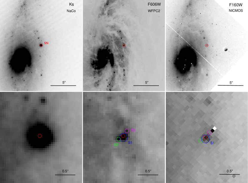
Figure 13.— Identification of the source at the SN location in pre-explosion HST images. North is up and East is to the left. Left column: combined $K_{s}$-band NaCo image from March 2010 showing the SN (red circle). Middle column: F606W-band WFPC2 image from February 1996. Right column: F160W-band NICMOS image from July 1997. In the zoomed-in images of the lower row the SN location is indicated by red circles with radius of three times the uncertainty in the relative astrometric solution. The locations of the sources S1, S2 and S3 detected in the F606W image are shown with blue, green and magenta circles, respectively. The sizes of the circles roughly indicate the source brightnesses. We associate S1 with the SN site. Only S1 is detected in the F160W image (right bottom panel).

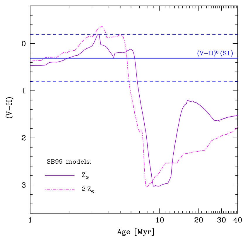
Figure 14.— Evolution of the $(V-H)$ color for synthetic stellar population models from Starburst99 assuming a single star-formation burst. The solid curve is for solar metallicity while the dot-dashed curve corresponds to twice-solar metallicity. Blue horizontal lines show the color of source S1 after correcting for reddening, with 1-$\sigma$ uncertainties indicated by the dashed lines. Dashed horizontal lines indicate 1-$\sigma$ uncertainties in the observed color.

4.3. Hydrodynamical models

One way to estimate the physical parameters of the SN progenitor as well as the energy release and radioactive material yield is by modelling the observed light curve and the photospheric velocity ($v_{\mathrm{ph}}$) evolution. We used the bolometric light curve calculated in Section 3.3 and the Fe II line velocity as a tracer for the photospheric velocity. Although in general the latter is a good assumption for SE SNe (Branch et al., 2002), as we showed in Section 3.4.1, for SN 2010as the photospheric velocity at early times may lie well below the Fe II velocity (see also the discussion below). For the hydrodynamical modelling we adopted an explosion time at the midpoint between the last non-detection and the discovery time, $t_{\mathrm{exp}}$ (see Section 2).

We used the one-dimensional LTE radiation hydrodynamics code previously presented by Bersten et al. (2011) to calculate a set of SN models. Helium stars with different masses calculated from a single stellar evolutionary code (Nomoto & Hashimoto, 1988) were adopted as pre-explosion configurations. These initial models are devoid of hydrogen and have a compact structure with radius $R<3\,R_{\odot}$. Note that although the spectra of SN 2010as show evidence of a thin H envelope (as shown in Section 3.4.1), the uncertainty on $t_{\mathrm{exp}}$ and the lack of an observed post-breakout cooling phase in the light curves prevent us from drawing conclusions about the extent of the envelope (see Bersten et al., 2012). We therefore focus our modelling only on the ⁵⁶Ni-powered part of the light curve where global properties such as explosion energy ($E$), ejected mass ($M_{\mathrm{ej}}$), and ⁵⁶Ni mass can be estimated.

The sensitivity of the light curve and $v_{\mathrm{ph}}$ evolution to $E$, $M_{\mathrm{ej}}$, ⁵⁶Ni mass and ⁵⁶Ni distribution has been previously studied in Bersten et al. (2012), and therefore it will not be described here. Nevertheless, we note that, for a given progenitor mass, $v_{\mathrm{ph}}$ imposes a stronger constraint on the energy than does the light curve on the explosion energy. This is because of the weak dependence of $v_{\mathrm{ph}}$ on the amount and distribution of ⁵⁶Ni. Figure 15 shows the hydrodynamical modelling of SN 2010as for three different initial configurations, namely for He stars of $3.3$ $M_{\odot}$ (HE$3.3$), 4 $M_{\odot}$ (HE4) and 5 $M_{\odot}$ (HE5). Such pre-SN configurations correspond to single stars with main-sequence masses of 12 $M_{\odot}$, 15 $M_{\odot}$ and 18 $M_{\odot}$, respectively. From the figure we see that the HE4 model provides the best representation of the observations (light curve and velocity together). The HE$3.3$ model is slightly overluminous, it produces an acceptable approximation of the light-curve shape. A more massive model (HE5) already produces a too wide light curve with an underluminous peak. The failure of the massive model resides in the difficulty of simultaneously fitting the light-curve width and the low expansion velocities. In particular for SN 2010as, even the Fe II line velocities are relatively low at early times. The width of the light curve grows with increasing pre-SN mass and also with decreasing $E$. For massive models, the low observed velocities require the energy to be relatively low, thus impeding the possibility of reducing the light-curve width.

Here we adopt HE4 as our preferred model, and the parameters used in the calculation shown in Figure 15 are an explosion energy of $E=7\times 10^{50}$ erg, an ejected mass of $M_{\mathrm{ej}}=2.5$ $M_{\odot}$, and a ⁵⁶Ni yield of about $0.12$ $M_{\odot}$. It is beyond the scope of this work to provide a comprehensive analysis of the uncertainties in the physical parameters. Given that the uncertainty in luminosity is nearly systematic (see Section 3.3), the light curve may shift vertically but its shape will remain fixed. The line velocities are not affected by the distance uncertainty. Since $E$ and $M_{\mathrm{ej}}$ both affect the shape of the light curve and the velocities, we expect that most of the luminosity uncertainty is transferred to the ⁵⁶Ni mass. To reproduce the rise of the light curve we assumed ⁵⁶Ni mixing up to 95% of the initial mass, although we note that this value has a large uncertainty given the uncertainty on $t_{\mathrm{exp}}$.

It is interesting to note that even if we could reproduce the light curve and the Fe II velocity evolution reasonably well, none of our models were able to reproduce the rather flat behavior of the Fe II velocity at early times, nor the even lower photospheric velocity derived from the SYNOW synthetic spectra (see Section 3.4.1). That analysis indicated that the photospheric velocity at early times could be better represented by He I or Mg II lines than by Fe II. Assuming He I velocity as the photospheric velocity, a very weak explosion with $E\lesssim 2\times 10^{50}$ erg is required to reproduce the low $v_{\mathrm{ph}}$. However, this leads to a very faint and wide light curve, in contradiction with the observations, even for our lowest-mass progenitor. Therefore, we conclude that if we use He I velocities we cannot find a model that reproduces the light curve and $v_{\mathrm{ph}}$ simultaneously under the current assumptions. In this sense we emphasize that our calculations assume spherical symmetry. It is possible that the peculiar behavior of He I velocities could be associated with departures from spherical symmetry in the explosion (Tanaka et al., 2009).

We also analyzed the possibility that SN 2010as was powered by a magnetar instead of the typical ⁵⁶Ni power. The motivations to explore a magnetar as the energy source were, first, that SN 2010as showed some spectroscopic similarities with SN 2005bf for which a magnetar was suggested to reproduce the unusual light-curve morphology (Maeda et al., 2007), and, second, that magnetar models produce flat photospheric velocity evolution (see Woosley, 2010; Kasen & Bildsten, 2010; Dessart et al., 2012b). We included the magnetar energy in our hydrodynamical code following the prescriptions of Woosley (2010) and Kasen & Bildsten (2010). The magnetar model depends mainly on two parameters, the intensity of the magnetic field and the initial rotation period of the neutron star. We tested different values of these parameters but we could not find a configuration that could reproduce the light-curve brightness and the rise time. In addition, we found that only powerful magnetars can affect the dynamics of the SN ejecta, and thereby produce a flat photospheric velocity evolution. However, this type of models produces super-luminous supernovae which are a few orders of magnitude more luminous than normal core-collapse SNe. We therefore exclude the possibility of a magnetar as the main source of power for SN 2010as. There may be other mechanisms besides a magnetar that lead to the formation of a shell inside the ejecta, and that may reproduce the observed velocity evolution. We plan to study this interesting possibility in the future.

In conclusion, by approximating photospheric velocities with Fe II line velocities, our analysis suggested a progenitor star with a He core of $\approx$4 $M_{\odot}$, which corresponds to a main sequence mass of $\approx$15 $M_{\odot}$ (based on the adopted initial model). The explosion released an energy of $E\approx 7\times 10^{50}$ erg and produced $0.12$ $M_{\odot}$ of ⁵⁶Ni. In addition, our modelling disfavored models with He core mass above 5 $M_{\odot}$, which implies a main sequence mass below 20 $M_{\odot}$. Such relatively low masses suggest a binary progenitor for SN 2010as since stellar winds alone would not produce enough mass loss to almost completely remove the H-rich envelope (see Puls et al., 2008). The formation of a dense shell could be a solution for the flattening of the line velocity evolution, although we did not provide a physical mechanism to account for the existence of such dense shell. Departures from spherical symmetry may also explain the low $v_{\mathrm{ph}}$.

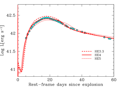
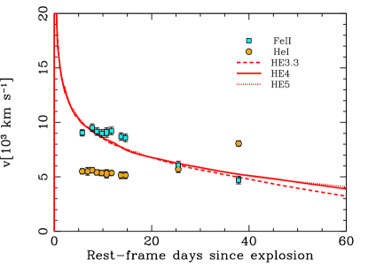
Figure 15.— (Top panel) Observed bolometric light curve of SN 2010as (circles) compared with the hydrodynamical models HE$3.3$ (dashed line), HE4 (solid line) and HE5 (dotted line). (Bottom panel) Evolution of the photospheric velocity for the same models as above compared with measured line velocities of Fe II (squares) and He I (circles).

4.4. Progenitor Mass

SN 2010as is one of the few H-poor SNe for which a pre-explosion source could be identified. In this case, however, the luminosity of the source is compatible with a massive stellar cluster rather than the specific progenitor object (see Section 4.2). Therefore, the estimation of the progenitor mass was rather indirect as it relied on assumptions on the star-formation history in the cluster and on the model-dependent link between cluster age and main-sequence mass of the most-massive star. From the color of the source we derived an age of the cluster, assuming a single star-formation burst. Provided the progenitor of SN 2010as was the most massive star in the cluster, and assuming single stellar evolution models, we were able to estimate the main-sequence mass of the progenitor to be above 28–29 $M_{\odot}$, depending on the adopted metallicity. This is roughly compatible with the progenitor being a Wolf-Rayet star that had lost most of its outer envelope via strong winds prior to explosion. If we relax the assumption of a single stellar burst, the age of the cluster could be older and that could imply masses slightly below the range of WR stars (see, e.g., Langer, 2012; Groh et al., 2013).

On the other hand, the hydrodynamical modelling provides constraints on the progenitor mass at the moment of the explosion, which can be associated to the ZAMS mass by assuming some stellar evolution model. Our analysis of Section 4.3 favors a low-mass object with a pre-SN mass below 5 $M_{\odot}$, in disagreement with a WR progenitor that would be more massive at explosion. However, this analysis relies in part on the assumption that the photospheric evolution can be traced by Fe II line velocities, which is questionable for SN 2010as. In addition, the models failed to reproduce the observed flat velocity evolution. This may indicate that other mechanisms need to be considered or that some of the model hypotheses, such as the spherical symmetry, may not be valid. These difficulties make the conclusions from the hydrodynamic modelling less accurate for this SN than what is usually the case.

The results from Sections 4.2 and 4.3 appear to be in contradiction. On the one hand, we found evidence for a young progenitor age while, on the other hand, the exploding object appeared to have a relatively low mass. Relaxing the main assumptions in each case, i.e., the spherical symmetry in the hydrodynamical calculations, and the single star-formation burst in the cluster age determination, the disagreement can be improved. We further measured the flux ratio of [Ca II] $\lambda$$\lambda$7291, to [O I] $\lambda$$\lambda$6300, 6363, which is indicative of the core mass, and thus of the ZAMS mass (Fransson & Chevalier, 1987, 1989). The spectrum at $+309$ days did not cover the [O I] completely. We assumed the profile to be symmetric, and measure the line flux as twice the flux of the blue component up to the central trough. The resulting [Ca II]/[O I] ratio was 0.95. This value is similar to, for example, those of SN 1996N and SN 2007Y (Stritzinger et al., 2009, and references therein), and it suggests a relatively low progenitor mass of $M_{\mathrm{ZAMS}}\lesssim 20$ $M_{\odot}$. Nevertheless, both pieces of evidence can be reconciled within the scenario of a close binary progenitor system. The recent suggestion that about 70% of the massive stars belong to interacting binary systems (Sana et al., 2012) makes this a reasonable possibility. As shown in the calculations of Yoon et al. (2010), interacting binaries with large initial masses of the primary stars ($\approx$25 $M_{\odot}$) may end their evolution with relatively low pre-SN masses ($\approx$4 $M_{\odot}$) after losing most of the envelope via Roche-lobe overflow. Moreover, the lifetime of the primary star would not be significantly altered by the mass-transfer processes because it is determined by the time-scale of nucleosynthesis in the stellar core. Therefore, the age of the system at the moment of explosion would also be compatible with the estimated cluster age.

5. The Family of Flat-Velocity Type IIb Supernovae

5.1. Transitional Type Ib/c SNe are Peculiar Type IIb SNe

Figures 16 to 19 show the spectroscopic comparison in the optical between SN 2010as and other SE SNe at four different epochs. Figure 20, additionally shows a comparison of available pre-maximum spectra of SE SNe in the NIR range. Comparison spectra were obtained from the The Weizmann interactive supernova data repository (Ofer & Gal-Yam, 2012). The overall spectral evolution of SN 2010as makes this object most similar to a group of transitional Type Ib/c SNe that were first introduced with the case of SN 1999ex (Hamuy et al., 2002; Stritzinger et al., 2002). Other objects with similar spectroscopic characteristics are SN 2005bf (Anupama et al., 2005; Tominaga et al., 2005; Folatelli et al., 2006) and 2007Y (Stritzinger et al., 2009). The similarities among these objects, in contrast with normal Type Ib SNe, are most clearly seen before maximum light, as shown in Figures 16 and 17. The distinguishing features among transitional Type Ib/c SNe is the weakness of He I lines, the strength of high-velocity Ca II absorptions, and the broad absorption near 6200 Å that we have attributed to H$\alpha$ for SN 2010as. Helium lines grow in strength until maximum light, while high-velocity Ca II components dominate before maximum and disappear after. SN 2010as shows particularly strong Ca II absorptions at all times. As shown in Figure 20, the pre-maximum NIR spectra of SN 2010as, as well as those of SN 1999ex, show weaker He I lines than the comparison Type Ib and IIb objects.

After maximum light (Figure 18) helium lines are clear in transitional Type Ib/c SNe, while the absorption near 6200 Å becomes weaker, as compared with typical Type IIb objects, and it appears blended with other lines. About three weeks after maximum (Figure 19), SN 2010as and 2005bf remain similar while SN 2007Y shows well-developed He I lines. The spectroscopic similarity among the former two objects is most striking if one considers the large differences in light-curve properties and luminosities (see Figure 8). We note that at day $+22$ SN 2005bf is near the main maximum in its light curve, while SN 2010as follows the usual post-maximum decline of SE SNe.

The group of transitional Type Ib/c SNe appears spectroscopically closer to Type IIb than to Type Ib objects. Furthermore, the presence of hydrogen seems to be ubiquitous among all these SNe. We have shown in Section 3.4.1 the identification of the 6200-Å absorption with H$\alpha$ for SN 2010as. The same identification has been suggested for SN 1999ex (Branch et al., 2006; Elmhamdi et al., 2006), SN 2005bf (Anupama et al., 2005; Folatelli et al., 2006; Parrent et al., 2007), and SN 2007Y (Stritzinger et al., 2009; Maurer et al., 2010). The latter object may be a link between transitional Type Ib/c SNe and Type IIb SNe, with lower H abundance, as suggested by its resemblance with SN 2008ax (see Figures 16 through 19). Finally, H$\alpha$ is present in the nebular spectra of SN 2005bf and SN 2007Y, and possibly in SN 2010as (see Figure 11). Hydrogen has also been suggested in early spectra of Type Ib SNe (see Elmhamdi et al., 2006), although the confusion is larger in this case between H$\alpha$ and Si II $\lambda$6355 (Hachinger et al., 2012). In the NIR range (see Figure 20), although P$\alpha$ is difficult to identify, hints of the presence of P$\beta$ are seen in SNe 2010as, 1999ex, 2011dh and 2008ax, but not in the Type Ib SN 2009jf.

The differences between transitional Type Ib/c SNe and standard Type Ib objects are further highlighted in Figures 21 and 22, where we show the pre-maximum evolution of He I $\lambda$5876 and H$\alpha$, respectively. The former line was chosen because it is the strongest He I line in the optical range. He I $\lambda$5876 appears relatively weaker and at lower velocity in transitional Type Ib/c and Type IIb SNe than in Type Ib objects. The strength and shape of the H$\alpha$ profile also shows greater resemblance between the former two groups.

From this analysis we conclude that transitional Type Ib/c SNe are in fact Type IIb SNe. However, they can be distinguished from standard Type IIb objects. Their most evident peculiarity is the early evolution of helium velocities. Figure 23 shows a comparison of He I $\lambda$5876 velocities for a sample of SE SNe. All the transitional Type Ib/c SNe can be distinguished by their low and flat early-time helium velocity evolution. This peculiar behavior was previously shown for SN 2005bf by Tominaga et al. (2005), and for SNe 1999ex and 2007Y by Taubenberger et al. (2011). Interestingly, the Type IIb SN 2011dh shows the same peculiarity. The flat—sometimes increasing—behavior at early time is in contrast with the typical velocity decline that is observed among SE SNe, including other Type IIb SNe and all Type Ib objects (see also Branch et al., 2002). A flattening of the He I $\lambda$5876 velocities can occur for SE SNe after maximum light, but this is preceded by a steep decline. Moreover, the maximum-light He I $\lambda$5876 velocities are lower for the flat-velocity objects than for the bulk of SE SNe. Values go from $\approx$5500 km s^-1 for SN 2010as in the lower extreme, to $\approx$8000 km s^-1 for SN 2007Y at the higher end. After maximum light, He I $\lambda$5876 velocities for these objects tend to increase. This may be due in part to contamination by Na I. The peculiarity of low and flat pre-maximum He I $\lambda$5876 velocity observed here cannot be explained by Na I contamination as this line is only about 800 km s^-1 to the red of the helium feature. We stress the fact that, for SN 2010as, the low and flat velocity evolution was a general feature of the photosphere—as defined in SYNOW—and not a peculiarity of the helium lines.

This indicates the existence of a family of Type IIb SNe that are characterized by low and flat expansion velocities before maximum light, most notably of helium lines, but presumably of the photosphere as a whole. The members of such family are listed in Table 10. We further propose to distinguish them from standard Type IIb objects with the name “Type fvIIb” (standing for “flat-velocity Type IIb”). We find no clear connection between this distinction based on early-time velocities, and the separation between compact and extended Type IIb SNe proposed by Chevalier & Soderberg (2010), based on radio observations. In terms of their expansion velocities, the prototypes of compact (SN 2008ax) and extended (SN 1993J) Type IIb SNe are very similar. Given the post-maximum weakness of the H$\alpha$ line in objects formerly identified as transitional Type Ib/c SNe, this may indicate that they represent a limit towards zero hydrogen abundance among Type IIb SNe. The remaining question is whether this tendency to zero hydrogen can be physically associated with the peculiar behavior of helium lines or if an additional mechanism should be invoked to account for such behavior.

5.2. On the Origin of Low and Flat Velocities

The most striking feature of the family of Type fvIIb SNe is the persistence of low expansion velocities. Considering also the presence of hydrogen and initial weakness of helium lines, we can characterize the spectroscopic evolution of these objects as a transition from “Type IIc” (i.e., with weak hydrogen and no helium) to Type IIb. As noted by Dessart et al. (2012a), this very unique behavior is not easy to attain by the models, as it requires the presence of a small amount of hydrogen in the outer layers, and a significant amount of helium that remains invisible at early times. In such a picture, helium lines grow as the He-rich region becomes heated, either by radioactive material, or by some other process that releases energy in its vicinity. Such an alternative process may be the onset of a magnetar (Dessart et al., 2011), although for SN 2010as and other normal-luminosity SNe, this is unlikely (see Section 4.3).

If we consider radioactive material as the heat source, then the degree of mixing with helium-rich material must play an important role (Dessart et al., 2012a). The IIc–IIb transition requires that mixing is moderate, so that helium excitation becomes significant only once the photosphere reaches the ⁵⁶Ni-rich layers. For Type fvIIb SNe, in order to maintain the velocity nearly constant, the increasing excitation of helium would possibly require an increasing $\gamma$-ray leakage from the ⁵⁶Ni-abundant region to the He-rich region, as suggested by Tominaga et al. (2005) for SN 2005bf. From spectropolarimetry of that SN, Tanaka et al. (2009) further suggested that mixing of ⁵⁶Ni with helium occurred in an aspherical, clumpy manner.

The nearly constant photospheric velocity is suggestive of the presence of a dense shell inside the SN ejecta. For different SNe, this shell would be formed at different velocities, as shown in Figure 23. If the differences are intrinsic, they may be related with a variation in the progenitor structure or a difference in the propagation of the explosive wave. The magnetar scenario, although it can naturally produce a dense shell within the ejecta, is not favored for SNe of normal luminosity and rise time. Alternatively, the variation of velocity levels may not be an intrinsic property but a consequence of a projection effect in an aspherical ejecta. In Section 3.4.2 we suggested an asymmetric distribution of the inner O-rich material in SN 2010as, due to the double peak of the [O I] emission. However, this type of features is not exclusively seen in SNe with flat velocities, and also the geometry implied by the nebular spectrum may not coincide with that of the outer ejecta that is observed near maximum light.

The helium velocity, and presumably the photospheric velocity, is different for different flat-velocity objects, as shown in Figure 23. The following sequence of increasing helium—and presumably photospheric—velocity is observed: SN 2010as–2005bf–1999ex–2011dh–2007Y. There is a hint of decreasing luminosities in the same direction, as seen in Table 10 and Figure 8. A larger sample is required to investigate whether such sequence becomes a correlation between luminosity and helium velocity. The large spectroscopic sample recently released by Modjaz et al. (2014) may serve to this purpose. Similarly, an increased sample and spectral modelling may provide clues as to whether hydrogen abundances reproduce the same sequence. From the strength of H$\alpha$ in the photospheric phase, this is not clear (see Figure 22), however the observed strength of H$\alpha$ in the nebular phase suggests that the amount hydrogen seen at late-time grows in the expected order.

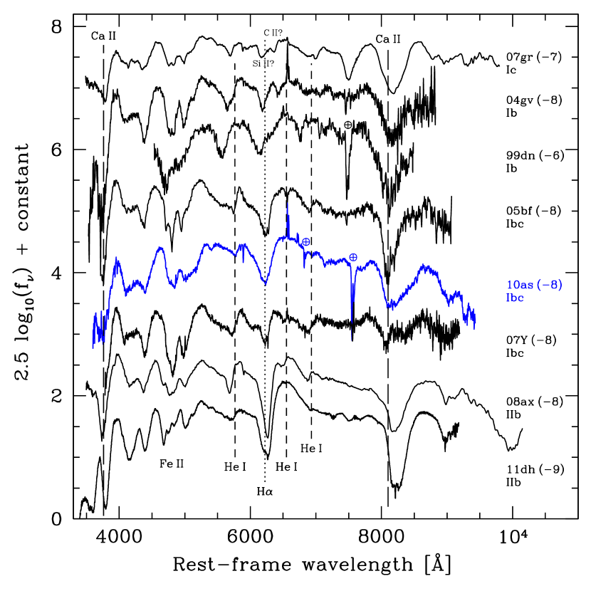
Figure 16.— Spectroscopic comparison between SN 2010as and other SE SNe at six to nine days before maximum. Labels on the right-hand of each spectrum indicate the SN name and type, and the epoch between parentheses. Vertical lines show the location of absorption lines of H I (dotted), He I (short-dashed) and Ca II (long-dashed), with a Doppler shift as measured for SN 2010as. Earth symbols indicate partially or uncorrected telluric absorptions.

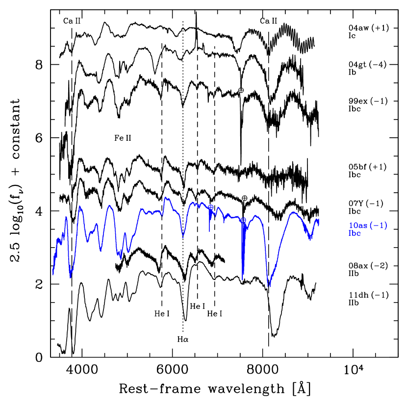
Figure 17.— Spectroscopic comparison between SN 2010as and other SE SNe around maximum light. Labels and symbols are as in Figure 16.

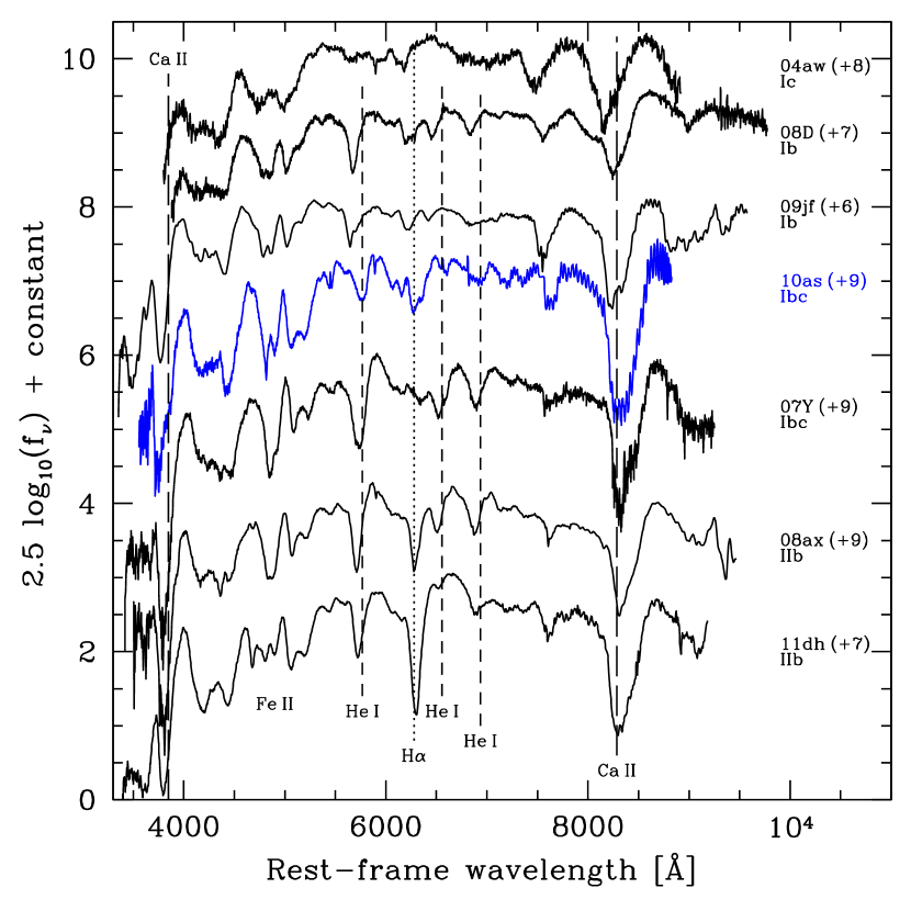
Figure 18.— Spectroscopic comparison between SN 2010as and other SE SNe at six to nine days after maximum light. Labels and symbols are as in Figure 16.

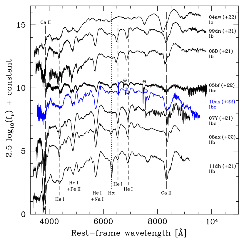
Figure 19.— Spectroscopic comparison between SN 2010as and other SE SNe at about three weeks after maximum light. Labels and symbols are as in Figure 16.

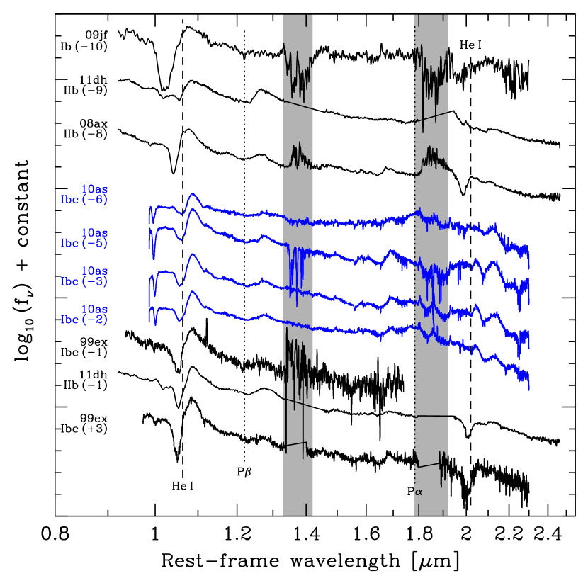
Figure 20.— Spectroscopic comparison between SN 2010as and other SE SNe in the NIR range. Labels on the left-hand side indicate the SN name, type and epoch relative to maximum light. Main He I lines are indicated by vertical dashed lines located at a velocity of 5700 km s^-1. Also shown with dotted lines are the expected locations of P$\alpha$ and P$\beta$ at a velocity of 14500 km s^-1. The gray bands indicate the regions where atmospheric transmission drops approximately below 50%.

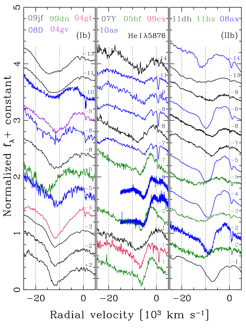
Figure 21.— Evolution of the He I $\lambda$5876 lines for SE SNe. Each graph shows three columns, separated into Type Ib, transitional Type Ib/c, and Type IIb SNe. The spectra are shown versus velocity relative to the rest wavelength of the line. Vertical dotted lines show 0, 10000 km s^-1 and 20000 km s^-1. Numerical labels on the right-hand side indicate the epoch of each spectrum in days with respect to $B$-band maximum light.

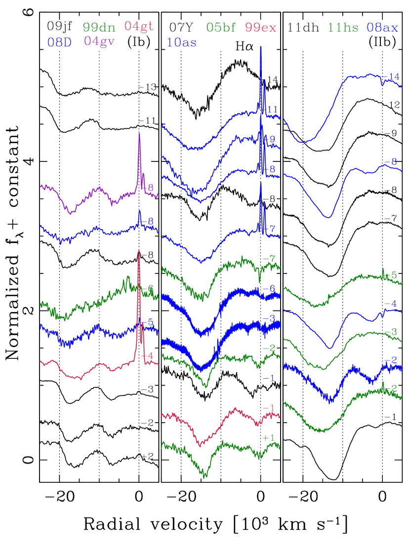
Figure 22.— Evolution of the H$\alpha$ lines for SE SNe. Each graph shows three columns, separated into Type Ib, transitional Type Ib/c, and Type IIb SNe. The spectra are shown versus velocity relative to the rest wavelength of the line. Vertical dotted lines show 0, 10000 km s^-1 and 20000 km s^-1. Numerical labels on the right-hand side indicate the epoch of each spectrum in days with respect to $B$-band maximum light.

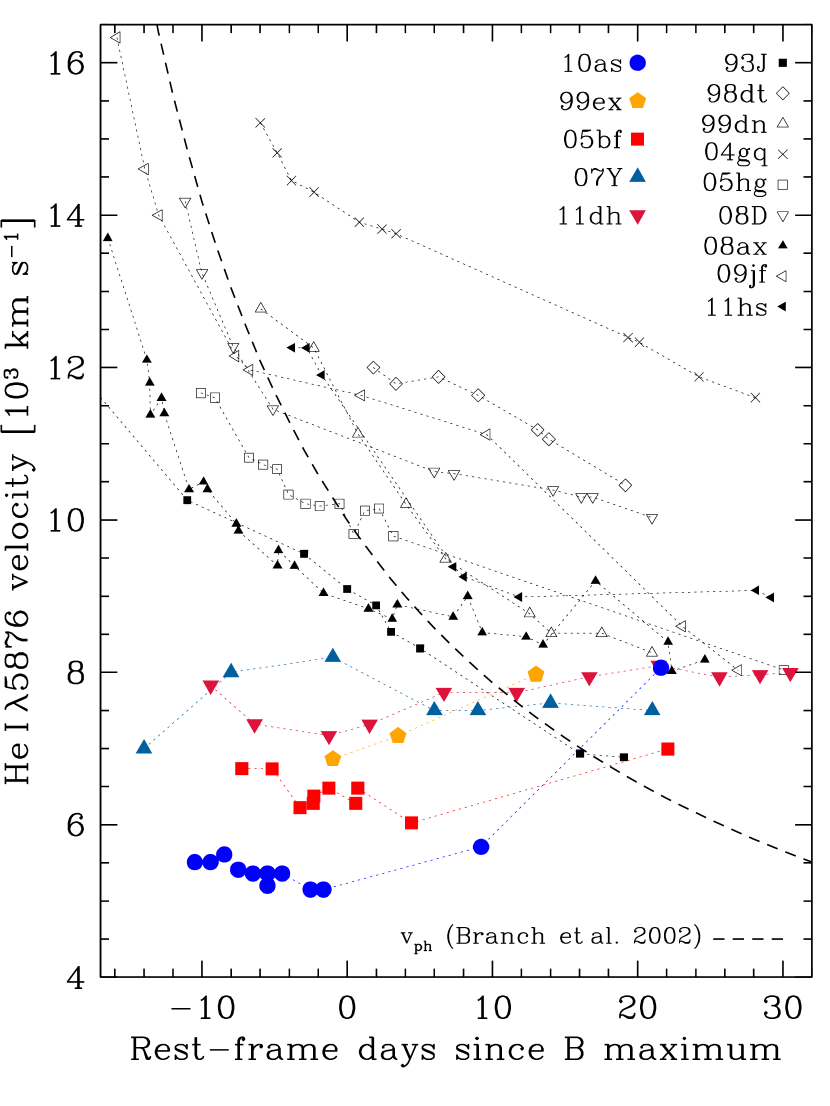
Figure 23.— Comparison of He I $\lambda$5876 velocities for transitional Type Ib/c SNe compared with other SE SNe. The black dashed curve shows the power-law evolution of $v_{\mathrm{ph}}$ that is typical of Type-Ib and Ic SNe, as derived by Branch et al. (2002). Objects shown in color have flat helium velocity evolution before they cross the power-law $v_{\mathrm{ph}}$ curve. Filled symbols indicate Type IIb SNe while open symbols correspond to Type Ib objects.

6. CONCLUSIONS

We have used extensive observations of the SE SN 2010as to characterize its photometric and spectroscopic evolution. The long-wavelength base of the photometry, from $B$ band to $K$ band, allowed us to compute several color indices and, from a comparison with colors of a sample of SE SNe, determine a non-standard reddening characterized by a low total-to-selective extinction coefficient of $R_{V}=1.5$. The optical and NIR photometry was used to integrate a bolometric light curve that was used to compare with hydrodynamic modelling. The spectra, obtained with a nearly nightly cadence before maximum light and with NIR coverage, allowed the identification of the main ions in the SN ejecta, and their approximate distribution in velocity space. Strong evidence of the presence of hydrogen was found. The evolution of the photospheric velocity was found to be peculiarly low and nearly constant in time since the earliest spectroscopy epochs at $-11$ days with respect to maximum light.

SN 2010as was associated with a young, massive stellar cluster present in archival HST images. This suggested a large ZAMS mass for the progenitor, roughly compatible with a WR star, under the assumption of a single star burst. In contrast with that, our hydrodynamical modelling showed that the explosion energy and pre-SN mass should be relatively low. Our best match model has $E\approx 7\times 10^{50}$ erg, $M_{\mathrm{pre-SN}}\approx 4$ $M_{\odot}$, and a ⁵⁶Ni yield of $\approx$$0.12$ $M_{\odot}$. However, the model fails to reproduce the observed flat and low velocity evolution. This may be due to a limitation of our one-dimensional prescription, or to a missing physical mechanism that may form a dense shell in the SN ejecta. In any case, the seeming inconsistency can be readily solved by considering an interacting binary progenitor scenario, where an initially massive star looses its envelope through mass transfer to the secondary star and reaches the pre-supernova stage at a young age but with a relatively low mass (Yoon et al., 2010; Bersten et al., 2014).

SN 2010as belongs to a small family of SE SNe listed in Table 10 that show peculiar spectroscopic properties, such as the transition from almost He-free to He-rich spectra, accompanied by low and nearly constant photospheric velocities near maximum light. Although some of these objects were previously classified as “transitional Type Ib/c” SNe, we have shown compelling evidence of the ubiquitous presence of hydrogen in this group, which calls for a Type IIb classification. However, they show a peculiar velocity evolution, so we have distinguished them as “flat-velocity Type IIb” (Type fvIIb) SNe. This group might represent the limit to zero hydrogen among Type IIb SNe, although this needs to be verified with spectral modelling.

The distinguishing property of approximately constant velocity for this family of SNe is suggestive of a dense shell in the ejecta. Velocities of different SNe are different and span the range between 6000 and 8000 km s^-1, with SN 2010as showing the lowest velocity in the group. The luminosities of Type fvIIb objects show a wide variety that might be correlated with the expansion velocities. This leaves the open questions of the origin of the low and flat velocities, and of its possible connection, or lack of, with luminosity. Continued studies of flat-velocity SNe may help to understand the mechanism behind their observed peculiarities, whether of physical origin related with the progenitor or the explosion properties, or as a consequence of a geometrical configuration.

Table 1Landolt-system $BVRI$ photometric sequence of field stars around SN 2010as.

Star	RA	Dec.	$B$	$V$	$R$	$I$
ID	(h:m:s)	(∘:′:′′)	(mag)	(mag)	(mag)	(mag)
1	15:49:47.411	$-29$:22:00.21	$15.303(035)$	$14.723(012)$	$14.638(657)$	$14.004(034)$
2	15:49:50.596	$-29$:21:30.22	$16.762(119)$	$16.091(012)$	$15.615(044)$	$15.191(035)$
3	15:49:59.370	$-29$:22:58.17	$14.393(053)$	$13.195(026)$	$12.541(028)$	$11.968(015)$
4	15:49:59.634	$-29$:22:46.47	$17.030(057)$	$16.223(022)$	$15.713(026)$	$15.220(017)$
5	15:50:01.984	$-29$:23:02.57	$15.087(061)$	$13.764(024)$	$13.024(023)$	$12.345(013)$
6	15:49:53.249	$-29$:24:32.93	$15.996(102)$	$14.835(047)$	$14.126(061)$	$13.451(043)$
7	15:49:43.791	$-29$:24:39.59	$16.004(062)$	$15.285(020)$	$14.843(024)$	$14.459(025)$
8	15:49:44.342	$-29$:23:52.40	$16.950(043)$	$16.258(020)$	$15.811(030)$	$15.408(021)$
9	15:49:37.469	$-29$:24:01.19	$15.229(054)$	$14.604(017)$	$14.211(029)$	$13.845(021)$
10	15:49:52.330	$-29$:20:26.20	$15.280(010)$	$16.169(015)$	$15.675(054)$	$15.534(528)$
11	15:49:53.861	$-29$:20:42.09	$15.280(010)$	$17.566(011)$	$16.868(057)$	$16.332(027)$
12	15:49:56.994	$-29$:26:00.37	$14.646(072)$	$13.889(019)$	$13.443(031)$	$13.061(018)$
13	15:50:05.146	$-29$:25:45.93	$16.380(043)$	$14.993(018)$	$14.215(017)$	$13.582(010)$
14	15:49:47.942	$-29$:24:53.56	$17.487(085)$	$16.669(027)$	$16.170(028)$	$15.727(027)$
15	15:49:46.103	$-29$:25:10.48	$17.517(076)$	$16.857(024)$	$16.424(030)$	$16.028(030)$
16	15:49:39.244	$-29$:24:13.54	$17.657(065)$	$16.794(024)$	$16.251(029)$	$15.747(023)$
17	15:49:37.704	$-29$:21:58.24	$15.431(057)$	$14.824(010)$	$14.399(039)$	$14.009(027)$
18	15:49:39.608	$-29$:20:27.26	$15.280(010)$	$15.982(059)$	$15.756(497)$	$15.089(040)$
19	15:49:37.335	$-29$:20:44.98	$15.280(010)$	$16.785(012)$	$16.305(050)$	$15.885(037)$

Note. — Uncertainties in parentheses are given in thousandth of a magnitude.

Table 2Sloan-system $g^{\prime}r^{\prime}i^{\prime}z^{\prime}$ photometric sequence of field stars around SN 2010as.

Star	RA	Dec.	$g^{\prime}$	$r^{\prime}$	$i^{\prime}$	$z^{\prime}$
ID	(h:m:s)	(∘:′:′′)	(mag)	(mag)	(mag)	(mag)
1	15:49:47.411	$-29$:22:00.21	$14.988(027)$	$14.584(013)$	$14.419(025)$	$14.374(031)$
2	15:49:50.596	$-29$:21:30.22	$16.450(028)$	$15.873(014)$	$15.628(025)$	$15.545(030)$
3	15:49:59.370	$-29$:22:58.17	$13.735(030)$	$12.836(014)$	$12.457(032)$	$12.264(035)$
4	15:49:59.634	$-29$:22:46.47	$16.617(033)$	$15.978(013)$	$15.669(027)$	$15.540(047)$
5	15:50:01.984	$-29$:23:02.57	$14.362(033)$	$13.342(012)$	$12.852(029)$	$12.599(037)$
6	15:49:53.249	$-29$:24:32.93	$\cdots$	$\cdots$	$\cdots$	$\cdots$
7	15:49:43.791	$-29$:24:39.59	$15.616(026)$	$15.089(012)$	$14.881(032)$	$14.813(035)$
8	15:49:44.342	$-29$:23:52.40	$16.591(027)$	$16.063(022)$	$15.836(051)$	$15.744(059)$
9	15:49:37.469	$-29$:24:01.19	$14.902(025)$	$14.445(015)$	$14.262(025)$	$14.210(028)$
10	15:49:52.330	$-29$:20:26.20	$16.563(034)$	$15.929(015)$	$15.692(031)$	$15.612(027)$
11	15:49:53.861	$-29$:20:42.09	$18.121(040)$	$17.166(021)$	$16.792(033)$	$16.618(039)$
12	15:49:56.994	$-29$:26:00.37	$14.216(030)$	$13.692(013)$	$13.483(032)$	$13.424(031)$
13	15:50:05.146	$-29$:25:45.93	$15.637(028)$	$14.546(013)$	$14.091(037)$	$13.844(043)$
14	15:49:47.942	$-29$:24:53.56	$17.062(030)$	$16.423(012)$	$16.165(018)$	$16.073(031)$
15	15:49:46.103	$-29$:25:10.48	$17.176(032)$	$16.665(014)$	$16.445(021)$	$16.364(030)$
16	15:49:39.244	$-29$:24:13.54	$17.232(040)$	$16.516(015)$	$16.198(021)$	$16.065(029)$
17	15:49:37.704	$-29$:21:58.24	$15.133(029)$	$14.649(014)$	$14.432(026)$	$14.360(028)$
18	15:49:39.608	$-29$:20:27.26	$16.287(028)$	$15.745(013)$	$15.513(032)$	$15.421(031)$
19	15:49:37.335	$-29$:20:44.98	$17.170(037)$	$16.572(011)$	$16.315(027)$	$16.230(035)$

Note. — Uncertainties in parentheses are given in thousandth of a magnitude.

Table 3Landolt-system $BVRI$ magnitudes of SN 2010as from PROMPT.

UT date	JD	$B$	$V$	$R$	$I$
(yyyy-mm-dd)	($-2400000$)	(mag)	(mag)	(mag)	(mag)
2010-03-20.20	55275.70	$18.166(066)$	$16.948(029)$	$16.560(025)$	$16.294(030)$
2010-03-21.20	55276.70	$17.730(057)$	$16.779(026)$	$16.330(022)$	$16.007(026)$
2010-03-22.20	55277.70	$17.523(046)$	$16.564(024)$	$16.113(020)$	$15.736(023)$
2010-03-24.10	55279.60	$17.210(043)$	$16.239(024)$	$15.790(019)$	$15.550(020)$
2010-03-25.20	55280.70	$16.995(039)$	$16.118(022)$	$15.719(018)$	$15.377(018)$
2010-03-25.20	55280.70	$16.974(038)$	$16.130(019)$	$15.703(017)$	$15.372(020)$
2010-03-26.30	55281.80	$16.859(035)$	$15.991(021)$	$15.545(017)$	$15.314(018)$
2010-03-28.20	55283.70	$16.704(032)$	$15.856(017)$	$15.445(014)$	$15.137(017)$
2010-03-28.20	55283.70	$16.722(033)$	$15.858(020)$	$15.440(016)$	$15.158(016)$
2010-03-29.20	55284.70	$16.634(035)$	$\cdots$	$\cdots$	$\cdots$
2010-03-30.20	55285.70	$16.605(030)$	$15.744(016)$	$15.308(015)$	$15.021(016)$
2010-03-30.20	55285.70	$16.632(030)$	$15.719(020)$	$15.303(016)$	$15.033(016)$
2010-03-31.20	55286.70	$16.580(031)$	$15.709(016)$	$15.253(014)$	$14.964(016)$
2010-04-01.20	55287.70	$16.580(031)$	$15.678(016)$	$15.183(014)$	$14.895(016)$
2010-04-02.20	55288.70	$16.593(035)$	$\cdots$	$\cdots$	$\cdots$
2010-04-03.20	55289.70	$16.656(032)$	$15.646(016)$	$15.130(013)$	$\cdots$
2010-04-04.20	55290.70	$16.815(036)$	$15.680(016)$	$15.153(013)$	$14.849(015)$
2010-04-06.20	55292.70	$17.013(039)$	$15.761(016)$	$15.182(013)$	$14.824(015)$
2010-04-08.20	55294.70	$17.250(043)$	$15.859(019)$	$15.189(015)$	$14.829(014)$
2010-04-09.20	55295.70	$17.351(044)$	$\cdots$	$\cdots$	$\cdots$
2010-04-10.20	55296.70	$17.469(045)$	$15.989(020)$	$15.329(015)$	$14.918(015)$
2010-04-12.30	55298.80	$17.647(054)$	$\cdots$	$\cdots$	$\cdots$
2010-04-15.20	55301.70	$17.940(059)$	$16.409(022)$	$15.620(016)$	$15.103(017)$
2010-04-19.20	55305.70	$18.289(067)$	$16.609(025)$	$15.804(018)$	$15.195(018)$
2010-04-21.20	55307.70	$18.405(067)$	$16.775(027)$	$15.922(019)$	$15.276(019)$
2010-04-26.20	55312.70	$18.724(090)$	$16.870(028)$	$16.149(021)$	$15.396(020)$
2010-05-08.30	55324.80	$18.950(084)$	$\cdots$	$\cdots$	$\cdots$
2010-05-12.10	55328.60	$18.992(102)$	$17.385(037)$	$16.726(028)$	$15.972(028)$
2010-05-19.10	55335.60	$19.000(087)$	$\cdots$	$\cdots$	$\cdots$
2010-05-30.10	55346.60	$\cdots$	$17.710(044)$	$17.226(036)$	$16.450(033)$
2010-06-05.10	55352.60	$19.194(096)$	$\cdots$	$\cdots$	$\cdots$
2010-06-12.00	55359.50	$19.345(118)$	$\cdots$	$\cdots$	$\cdots$
2010-07-12.00	55389.50	$\cdots$	$18.412(060)$	$18.189(059)$	$17.199(044)$

Note. — Uncertainties in parentheses are given in thousandth of a magnitude.

Table 4Sloan-system $g^{\prime}r^{\prime}i^{\prime}z^{\prime}$ magnitudes of SN 2010as from PROMPT.

UT date	JD	$g^{\prime}$	$r^{\prime}$	$i^{\prime}$	$z^{\prime}$
(yyyy-mm-dd)	($-2400000$)	(mag)	(mag)	(mag)	(mag)
2010-03-19.73	55275.24	$17.544(034)$	$\cdots$	$\cdots$	$\cdots$
2010-03-20.91	55276.40	$17.316(035)$	$16.493(021)$	$\cdots$	$\cdots$
2010-03-21.75	55277.25	$17.039(028)$	$\cdots$	$\cdots$	$\cdots$
2010-03-23.66	55279.15	$16.689(022)$	$16.026(016)$	$15.979(019)$	$16.115(032)$
2010-03-24.74	55280.24	$16.546(020)$	$15.920(015)$	$15.863(017)$	$15.970(029)$
2010-03-25.79	55281.29	$16.426(020)$	$15.796(015)$	$15.758(016)$	$15.817(027)$
2010-03-26.73	55282.22	$16.362(018)$	$15.725(014)$	$15.689(016)$	$15.719(026)$
2010-03-27.73	55283.24	$16.271(019)$	$15.641(013)$	$15.630(015)$	$15.651(025)$
2010-03-28.74	55284.24	$16.233(018)$	$15.582(013)$	$15.511(015)$	$15.532(025)$
2010-03-29.75	55285.25	$16.179(017)$	$15.516(014)$	$15.486(016)$	$15.497(024)$
2010-03-30.73	55286.23	$16.151(017)$	$15.461(013)$	$15.387(016)$	$15.437(025)$
2010-03-31.73	55287.22	$16.140(017)$	$15.448(013)$	$15.408(015)$	$15.390(025)$
2010-04-01.72	55288.22	$16.145(018)$	$15.384(020)$	$15.346(026)$	$15.357(051)$
2010-04-02.72	55289.22	$16.146(018)$	$15.400(013)$	$15.335(018)$	$15.374(028)$
2010-04-03.71	55290.21	$16.203(017)$	$15.381(012)$	$15.276(013)$	$15.321(022)$
2010-04-04.71	55291.21	$\cdots$	$15.394(012)$	$15.265(014)$	$15.345(024)$
2010-04-05.71	55292.21	$16.327(019)$	$15.442(013)$	$15.300(013)$	$15.311(021)$
2010-04-06.71	55293.21	$16.371(020)$	$15.457(012)$	$15.277(014)$	$15.354(022)$
2010-04-07.73	55294.23	$16.471(024)$	$\cdots$	$\cdots$	$\cdots$
2010-04-08.71	55295.21	$16.587(022)$	$15.517(012)$	$15.353(014)$	$15.354(024)$
2010-04-10.70	55297.20	$16.762(022)$	$15.649(015)$	$\cdots$	$\cdots$
2010-04-11.70	55298.20	$16.825(024)$	$15.702(013)$	$15.446(015)$	$15.481(023)$
2010-04-14.69	55301.19	$17.113(026)$	$15.881(015)$	$15.594(015)$	$15.615(025)$
2010-04-18.67	55305.17	$17.334(028)$	$16.101(016)$	$15.689(016)$	$15.848(027)$
2010-04-20.67	55307.17	$17.512(031)$	$16.238(017)$	$15.796(017)$	$15.836(028)$
2010-04-25.66	55312.16	$17.758(036)$	$16.433(021)$	$16.047(020)$	$15.988(031)$
2010-05-04.62	55321.12	$\cdots$	$16.852(025)$	$16.267(021)$	$\cdots$
2010-05-07.71	55324.21	$18.099(043)$	$\cdots$	$16.394(027)$	$16.369(030)$
2010-05-11.74	55328.24	$18.169(046)$	$\cdots$	$\cdots$	$\cdots$
2010-05-18.60	55335.10	$18.272(045)$	$\cdots$	$\cdots$	$\cdots$
2010-06-04.62	55352.12	$18.376(048)$	$\cdots$	$\cdots$	$\cdots$
2010-06-06.60	55354.10	$\cdots$	$\cdots$	$16.980(032)$	$16.983(050)$
2010-06-11.59	55359.09	$\cdots$	$17.496(033)$	$17.177(033)$	$17.300(061)$
2010-06-22.52	55370.02	$\cdots$	$17.644(040)$	$17.383(043)$	$\cdots$

Note. — Uncertainties in parentheses are given in thousandth of a magnitude.

Table 52MASS-system $JHK$ photometric sequence of field stars around SN 2010as.

Star	RA	Dec.	$J$	$H$	$K$
ID	(h:m:s)	(∘:′:′′)	(mag)	(mag)	(mag)
2	15:49:50.596	$-29$:21:30.22	$14.588(024)$	$14.238(044)$	$14.075(058)$
8	15:49:44.342	$-29$:23:52.40	$14.859(047)$	$14.485(061)$	$14.471(083)$
10	15:49:52.330	$-29$:20:26.20	$14.694(041)$	$14.298(049)$	$14.118(064)$
11	15:49:53.861	$-29$:20:42.09	$15.619(066)$	$14.850(067)$	$14.788(106)$
14	15:49:47.942	$-29$:24:53.56	$15.139(053)$	$14.604(055)$	$14.399(081)$
15	15:49:46.103	$-29$:25:10.48	$15.472(073)$	$15.228(109)$	$14.918(134)$
16	15:49:39.244	$-29$:24:13.54	$14.931(040)$	$14.466(058)$	$14.356(078)$
18	15:49:39.608	$-29$:20:27.26	$14.440(038)$	$14.117(048)$	$14.019(065)$
19	15:49:37.335	$-29$:20:44.98	$15.366(051)$	$14.824(068)$	$14.815(118)$

Note. — Uncertainties in parentheses are given in thousandth of a magnitude.

Table 62MASS-system $JHK$ magnitudes of SN 2010as from GROND.

UT date	JD	$J$	$H$	$K$
(yyyy-mm-dd)	($-2400000$)	(mag)	(mag)	(mag)
2010-03-21.89	55277.39	$15.385(055)$	$15.607(068)$	$15.774(152)$
2010-03-22.85	55278.35	$15.149(025)$	$15.130(046)$	$15.302(082)$
2010-03-24.89	55280.39	$15.097(017)$	$14.982(030)$	$15.082(071)$
2010-03-26.91	55282.41	$14.956(016)$	$14.798(023)$	$14.804(056)$
2010-03-29.91	55285.41	$14.667(012)$	$14.637(020)$	$14.513(044)$
2010-04-01.85	55288.36	$14.512(014)$	$14.489(018)$	$14.413(043)$
2010-04-04.82	55291.32	$\cdots$	$\cdots$	$14.296(042)$
2010-04-06.92	55293.42	$14.413(013)$	$14.253(020)$	$14.352(043)$
2010-04-09.92	55296.42	$14.384(013)$	$14.245(015)$	$14.286(037)$
2010-04-10.91	55297.41	$14.374(011)$	$14.235(016)$	$14.374(039)$
2010-04-13.70	55300.20	$14.468(013)$	$14.246(017)$	$\cdots$
2010-04-16.72	55303.22	$14.680(061)$	$14.399(094)$	$\cdots$
2010-04-17.74	55304.24	$14.623(014)$	$14.333(024)$	$\cdots$
2010-04-20.90	55307.40	$\cdots$	$14.512(019)$	$\cdots$
2010-04-23.92	55310.42	$14.812(020)$	$14.499(023)$	$14.422(052)$
2010-04-25.91	55312.42	$\cdots$	$14.605(021)$	$14.441(039)$
2010-04-28.92	55315.42	$\cdots$	$14.659(023)$	$14.588(051)$
2010-05-02.92	55319.42	$\cdots$	$\cdots$	$14.781(057)$
2010-05-07.93	55324.43	$15.270(024)$	$14.967(038)$	$14.800(050)$
2010-05-10.87	55327.37	$15.456(023)$	$15.011(030)$	$15.112(060)$
2010-05-19.76	55336.26	$15.645(033)$	$15.266(036)$	$15.634(126)$
2010-05-22.71	55339.21	$15.650(038)$	$15.357(049)$	$15.585(117)$
2010-05-29.70	55346.19	$15.980(045)$	$15.674(065)$	$15.685(110)$
2010-06-01.71	55349.21	$16.003(060)$	$15.757(087)$	$15.735(164)$
2010-06-04.55	55352.06	$16.040(059)$	$16.001(097)$	$15.857(144)$
2010-06-11.70	55359.19	$16.210(058)$	$16.106(100)$	$16.174(289)$
2010-06-13.46	55360.96	$16.042(067)$	$15.900(110)$	$\cdots$
2010-06-21.46	55368.96	$16.273(096)$	$16.322(168)$	$\cdots$
2010-06-29.58	55377.08	$16.442(107)$	$16.246(121)$	$16.756(259)$
2010-07-11.49	55388.99	$16.610(072)$	$\cdots$	$\cdots$
2010-07-19.46	55396.96	$17.168(143)$	$16.945(281)$	$\cdots$
2010-07-29.47	55406.97	$17.245(153)$	$\cdots$	$\cdots$
2010-09-14.48	55453.98	$17.240(217)$	$\cdots$	$\cdots$
2011-02-17.89	55610.39	$18.163(328)$	$\cdots$	$\cdots$

Note. — Uncertainties in parentheses are given in thousandth of a magnitude.

Table 7Spectroscopic observations of SN 2010as.

Date	JD	Epoch	Instrument	Wavelength	Airmass	Exposure
	$-2455000$	(days)		Range (nm)		(s)
(1)	(2)	(3)	(4)	(5)	(6)	(7)
2010-03-20	$275.80$	$-10.50$	WFCCD	$368-926$	$1.062$	2400
2010-03-21	$276.90$	$-9.41$	GMOS-S	$520-949$	$1.028$	600
2010-03-22	$277.85$	$-8.47$	WFCCD	$360-949$	$1.002$	1800
2010-03-23	$278.82$	$-7.51$	WFCCD	$360-949$	$1.025$	1800
2010-03-24	$279.83$	$-6.50$	WFCCD	$360-949$	$1.011$	1800
2010-03-25	$280.83$	$-5.50$	X-Shooter	$320-2500$	$1.005$	600
2010-03-25	$280.84$	$-5.50$	WFCCD	$368-926$	$1.003$	2700
2010-03-26	$281.85$	$-4.49$	X-Shooter	$320-2500$	$1.008$	480
2010-03-28	$283.83$	$-2.53$	X-Shooter	$320-2500$	$1.005$	480
2010-03-29	$284.73$	$-1.64$	X-Shooter	$320-2500$	$1.215$	600
2010-04-09	$295.67$	$9.22$	GHTS	$358-889$	$1.37$	600
2010-04-22	$308.16$	$21.62$	GMOS-S	$358-963$	$1.20$	900
2010-07-08	$385.71$	$98.61$	GMOS-S	$358-963$	$1.50$	2000
2010-07-23	$400.60$	$113.39$	GHTS	$353-885$	$1.07$	1800
2010-08-02	$410.55$	$123.27$	GMOS-S	$358-895$	$1.06$	1800
2010-08-05	$413.48$	$126.17$	GHTS	$354-886$	$1.0$	900
2011-02-05	$597.87$	$309.23$	IMACS	$398-1006$	$1.244$	1800

Note. — Columns: (1) UT date of observation; (2) Julian date of middle of observation; (3) Epoch in rest-frame days since the time of $B$-band maximum light; (4) Instrument name; (5) Wavelength range of spectrum in nm; (6) Airmass at the mid-point of the observation; (7) Total exposure time in seconds.

Table 8Light-curve parameters of SN 2010as derived from polynomial fits.

Filter	JDmax	$m_{\mathrm{max}}$	rms	Npt	$M_{\mathrm{max}}$
	$-2455000$	(mag)	(mag)		(mag)
(1)	(2)	(3)	(4)	(5)	(6)
$B$	$286.38\pm 0.5$	$16.583\pm 0.018$	$0.025$	20	$-17.26\pm 0.44$
$V$	$288.78\pm 0.5$	$15.667\pm 0.009$	$0.019$	19	$-17.59\pm 0.39$
$R$	$290.89\pm 0.5$	$15.157\pm 0.008$	$0.026$	19	$-17.85\pm 0.38$
$I$	$292.40\pm 0.5$	$14.837\pm 0.008$	$0.022$	18	$-17.85\pm 0.37$
$g^{\prime}$	$287.37\pm 0.5$	$16.138\pm 0.010$	$0.012$	19	$-17.49\pm 0.42$
$r^{\prime}$	$289.87\pm 0.5$	$15.397\pm 0.006$	$0.014$	21	$-17.68\pm 0.38$
$i^{\prime}$	$291.69\pm 0.5$	$15.298\pm 0.007$	$0.025$	21	$-17.50\pm 0.37$
$z^{\prime}$	$291.09\pm 0.5$	$15.324\pm 0.010$	$0.021$	20	$-17.23\pm 0.36$
$J$	$295.03\pm 0.5$	$14.400\pm 0.010$	$0.064$	15	$-17.99\pm 0.36$
$H$	$297.74\pm 1.0$	$14.250\pm 0.011$	$0.039$	17	$-18.06\pm 0.36$
$K$	$298.75\pm 1.0$	$14.256\pm 0.034$	$0.091$	20	$-18.00\pm 0.36$
Bol.	$287.99\pm 0.5$	$14.678\pm 0.005$	$0.013$	32	$-17.48\pm 0.36$

Note. — Columns: (1) Filter name; (2) Julian date of maximum light. Uncertainties were estimated from the data sampling; (3) Apparent magnitude at maximum light, with no extinction correction applied. Uncertainties were computed from uncertainties in the fit parameters; (4) Root-mean-square of the data points around the fit; (5) Number of data points used in the fit; (6) Absolute peak magnitude in each band $X$, $M_{\mathrm{max}}(X)=m_{\mathrm{max}}(X)\,-\,A_{\mathrm{Gal}}(X)\,-\,A_{\mathrm{host}}(X)\,-\,\mu$, with Galactic extinction $A_{\mathrm{Gal}}(X)$ from $E(B-V)_{\mathrm{Gal}}=0.151$ mag and $R^{\mathrm{Gal}}_{V}=3.1$, host-galaxy extinction $A_{\mathrm{host}}(X)$ from $E(B-V)_{\mathrm{host}}=0.42\pm 0.1$ mag and $R^{\mathrm{host}}_{V}=1.5$, and distance modulus $\mu=32.16\pm 0.36$ mag.

Table 9Black-body fits and bolometric light curve of SN 2010as.

UT date	JD	$T_{\mathrm{BB}}$	$R_{\mathrm{BB}}$	$\log(L_{B\rightarrow K})$	$\log(L_{\mathrm{Bol}})$
(yyyy-mm-dd)	($-2400000$)	(K)	($10^{15}$ cm)	(erg s-1)	(erg s-1)
2010-03-19.70	$55275.20$	$10023\pm 895$	$0.70\pm 0.08$	$41.75$	$41.87$
2010-03-20.70	$55276.20$	$12013\pm 919$	$0.62\pm 0.05$	$41.83$	$41.97$
2010-03-21.70	$55277.20$	$10063\pm 604$	$0.86\pm 0.06$	$41.92$	$42.06$
2010-03-22.85	$55278.35$	$8659\pm 409$	$1.15\pm 0.06$	$41.99$	$42.14$
2010-03-23.70	$55279.20$	$8923\pm 429$	$1.17\pm 0.06$	$42.04$	$42.18$
2010-03-24.70	$55280.20$	$9296\pm 461$	$1.18\pm 0.06$	$42.09$	$42.24$
2010-03-25.70	$55281.20$	$9423\pm 472$	$1.22\pm 0.06$	$42.14$	$42.29$
2010-03-26.73	$55282.22$	$9207\pm 445$	$1.30\pm 0.06$	$42.16$	$42.32$
2010-03-27.70	$55283.20$	$9171\pm 437$	$1.35\pm 0.06$	$42.19$	$42.35$
2010-03-28.74	$55284.24$	$9148\pm 431$	$1.41\pm 0.07$	$42.22$	$42.38$
2010-03-29.70	$55285.20$	$8938\pm 405$	$1.49\pm 0.07$	$42.24$	$42.40$
2010-03-30.70	$55286.20$	$8984\pm 405$	$1.52\pm 0.07$	$42.26$	$42.41$
2010-03-31.70	$55287.20$	$8827\pm 388$	$1.57\pm 0.07$	$42.28$	$42.42$
2010-04-01.72	$55288.22$	$8718\pm 373$	$1.62\pm 0.07$	$42.29$	$42.43$
2010-04-02.70	$55289.20$	$8421\pm 347$	$1.69\pm 0.07$	$42.29$	$42.43$
2010-04-03.70	$55290.20$	$8038\pm 306$	$1.80\pm 0.07$	$42.29$	$42.41$
2010-04-04.71	$55291.21$	$7676\pm 276$	$1.90\pm 0.08$	$42.28$	$42.40$
2010-04-05.70	$55292.20$	$7460\pm 255$	$1.96\pm 0.08$	$42.27$	$42.38$
2010-04-06.71	$55293.21$	$7248\pm 236$	$2.02\pm 0.08$	$42.26$	$42.37$
2010-04-07.70	$55294.20$	$6992\pm 216$	$2.10\pm 0.08$	$42.25$	$42.35$
2010-04-08.71	$55295.21$	$6744\pm 198$	$2.18\pm 0.08$	$42.23$	$42.33$
2010-04-09.70	$55296.20$	$6503\pm 182$	$2.26\pm 0.08$	$42.22$	$42.31$
2010-04-10.70	$55297.20$	$6440\pm 176$	$2.25\pm 0.08$	$42.20$	$42.29$
2010-04-11.70	$55298.20$	$6392\pm 175$	$2.22\pm 0.08$	$42.17$	$42.26$
2010-04-13.70	$55300.20$	$6315\pm 169$	$2.14\pm 0.08$	$42.13$	$42.21$
2010-04-14.70	$55301.20$	$6414\pm 184$	$1.98\pm 0.08$	$42.10$	$42.19$
2010-04-16.72	$55303.22$	$6360\pm 189$	$1.88\pm 0.08$	$42.06$	$42.14$
2010-04-17.74	$55304.24$	$5997\pm 150$	$2.11\pm 0.07$	$42.05$	$42.13$
2010-04-18.70	$55305.20$	$5849\pm 143$	$2.16\pm 0.08$	$42.04$	$42.12$
2010-04-20.70	$55307.20$	$5527\pm 129$	$2.33\pm 0.08$	$42.00$	$42.08$
2010-04-23.92	$55310.42$	$5181\pm 119$	$2.50\pm 0.09$	$41.96$	$42.04$
2010-04-25.70	$55312.20$	$5128\pm 116$	$2.47\pm 0.08$	$41.94$	$42.01$
2010-05-07.93	$55324.43$	$5230\pm 127$	$2.02\pm 0.07$	$41.78$	$41.87$
2010-05-10.87	$55327.37$	$5472\pm 135$	$1.78\pm 0.06$	$41.74$	$41.83$
2010-05-11.70	$55328.20$	$5442\pm 143$	$1.78\pm 0.07$	$41.73$	$41.82$
2010-05-17.70	$55334.20$	$5700\pm 154$	$1.55\pm 0.06$	$41.68$	$41.77$
2010-05-19.76	$55336.26$	$5722\pm 161$	$1.51\pm 0.06$	$41.66$	$41.75$
2010-05-30.10	$55346.60$	$6052\pm 197$	$1.22\pm 0.06$	$41.56$	$41.65$
2010-06-05.10	$55352.60$	$6349\pm 238$	$1.06\pm 0.06$	$41.51$	$41.61$
2010-06-12.00	$55359.50$	$6440\pm 265$	$0.97\pm 0.06$	$41.45$	$41.55$
2010-06-22.52	$55370.02$	$6973\pm 344$	$0.75\pm 0.06$	$41.38$	$41.47$
2010-07-12.00	$55389.50$	$6275\pm 508$	$0.82\pm 0.10$	$41.23$	$41.32$

Table 10Properties of the flat-velocity Type IIb SNe.

SN	Orig.	$v_{\mathrm{He}}({\mathrm{max}})$	$M_{V}({\mathrm{max}})$	Type	Phot.
name	type	($10^{3}$ km s-1)	(mag)	refs.	refs.
(1)	(2)	(3)	(4)	(5)	(6)
1999ex	Ib/c	$6.93\pm 0.21$	$-17.49\pm 0.40$	$a$	$b$
2005bf	Ib/c	$6.31\pm 0.08$	$-17.40\pm 0.31$	$c$	$c$
2007Y	Ib/c, IIb	$8.23\pm 0.38$	$-16.38\pm 0.34$	$d$, $e$	$d$
2010as	$\cdots$	$5.41\pm 0.12$	$-17.59\pm 0.39$	$\cdots$	$\cdots$
2011dh	IIb	$7.24\pm 0.14$	$-17.08\pm 0.34$	$f$, $g$	$g$

Note. — Columns: (1) SN name; (2) Original classification from the literature (when different types were found, they are all listed); (3) Velocity of the He I $\lambda$5876 line at $B$-band maximum light. Values obtained from straight-line fits to the data in the epoch range of $[-10:+10]$ days; (4) Reddening-corrected absolute peak magnitude in $V$ band. Distances and Galactic reddening adopted from NED, apparent peak magnitudes and host-galaxy reddening adopted from the references given in column (6); (5) References for the spectral typing of column (2); (6) References for the photometric information used to calculate $M_{V}({\mathrm{max}})$. References: $a$ - Hamuy et al. (2002); $b$ - Stritzinger et al. (2002); $c$ - Folatelli et al. (2006); $d$ - Stritzinger et al. (2009); $e$ - Maurer et al. (2010); $f$ - Arcavi et al. (2011); $g$ - Ergon et al. (2014).

References

- Anupama et al. (2005) Anupama, G. C., et al. 2005, ApJ, 631, 125
- Arcavi et al. (2011) Arcavi, I., et al. 2011, ApJ, 742, 18
- Asplund et al. (2009) Asplund, M., et al. 2009, ARA&A, 47, 481
- Benvenuto et al. (2013) Benvenuto, O. G., Bersten, M. C., & Nomoto, K. 2013, ApJ, 762, 74
- Bersten& Hamuy (2009) Bersten, M. C., & Hamuy, M. 2009, ApJ, 701, 200
- Bersten et al. (2011) Bersten, M. C., Benvenuto, O., & Hamuy, M. 2011, ApJ, 729, 61
- Bersten et al. (2012) Bersten, M. C., et al. 2012, ApJ, 757, 31
- Bersten et al. (2014) Bersten, M. C., et al. 2014, arXiv:1403.7288
- Bohlin & Gilliland (2004a) Bohlin, R. C., & Gilliland, R. L. 2004, AJ, 127, 3508
- Branch et al. (2002) Branch, D., et al. 2002, ApJ, 566, 1005
- Branch et al. (2006) Branch, D., et al. 2006, PASP, 118, 791
- Bufano et al. (2009) Bufano, F., et al. 2009, ApJ, 700, 1456
- Bufano et al. (2014) Bufano, F., et al. 2014, MNRAS, 439, 1807
- Cardelli et al. (1989) Cardelli, J. A., Clayton, G. C., & Mathis, J .S. 1989, ApJ, 345, 245
- Chevalier & Soderberg (2010) Chevalier, R. A., & Soderberg, A. M. 2010, ApJ,711, 40
- Clemens et al. (2004) Clemens, J. C., Crain, J. A., & Anderson, R. 2004, in The Goodman spectrograph, Proc. SPIE 5492, Ground-based Instrumentation for Astronomy, 331
- Clocchiatti et al. (2011) Clocchiatti, A., et al. 2011, AJ, 141, 163
- Dessart et al. (2011) Dessart, L. C., et al. 2011, MNRAS, 414, 2985
- Dessart et al. (2012a) Dessart, L. C., et al. 2012, MNRAS, 424, 2139
- Dessart et al. (2012b) Dessart, L. C., et al. 2012, MNRAS, 426, L76
- De Vaucouleurs et al. (1991) De Vaucouleurs, G., et al. in Third Reference Catalogue of Bright Galaxies. Volume I: Explanations and references. Volume II: Data for galaxies between 0h and 12h. Volume III: Data for galaxies between 12h and 24h.
- Dressler et al. (2011) Dressler, A., et al. 2011, PASP, 123, 288
- Drout et al. (2011) Drout, M. R., et al. 2011, ApJ, 753, 180
- Elmhamdi et al. (2006) Elmhamdi, A., et al. 2006, A&A, 450, 305
- Ergon et al. (2014) Ergon, M., et al. 2014, A&A, 562, A17
- Fagotto et al. (1994a) Fagotto, F., et al. 1994a, A&AS, 104, 365
- Folatelli et al. (2006) Folatelli, G., et al. 2006, ApJ, 641, 1039
- Fransson & Chevalier (1987) Fransson, C., & Chevalier, R. A. 1987, ApJ, 322, 15
- Fransson & Chevalier (1989) Fransson, C., & Chevalier, R. A. 1989, ApJ, 343, 323
- Garstang (1962) Garstang, R. H. 1962, MNRAS, 124, 321
- Georgy et al. (2009) Georgy, C., et al. 2009, A&A, 502, 611
- Greiner et al. (2008) Greiner, J., et al. 2008, PASP, 120, 405
- Groh et al. (2013) Groh, J. H., et al. 2013, A&A, 558, A131
- Hachinger et al. (2012) Hachinger, S., et al. 2012, MNRAS, 422, 70
- Hamuy et al. (2002) Hamuy, M., et al. 2002, AJ, 124, 417
- Hamuy et al. (2006) Hamuy, M., et al. 2006, PASP, 118, 2
- Hamuy et al. (2012) Hamuy, M., et al. 2012, Mem. Soc. Astron. Italiana, 83, 388
- Heger et al. (2003) Heger, A., et al. 2003, ApJ, 591, 288
- Hook et al. (2004) Hook, I., et al. 2004, PASP, 116, 425
- Hunter et al. (2009) Sahu, D. J., et al. 2009, A&A, 508, 371
- Kasen & Bildsten (2010) Kasen, D., & Bildsten, L. 2010, ApJ, 717, 245
- Ketchum et al. (2008) Ketchum, W., Baron, E., & Branch, D. 2008, ApJ, 674, 371
- Krist et al. (2011) Krist, J. E., Hook, R. N., & Stoehr, F. 2011, SPIE, 8127, 16
- Landolt (1992) Landolt, A. U. 1992, AJ, 104, 340
- Langer (2012) Langer, N. 2012, ARA&A, 50, 107
- Leitherer et al. (1999) Leitherer, C., et al. 1999, ApJS, 123, 3
- Leloudas et al. (2011) Leloudas, G. et al. 2011, A&A, 530, 95
- Lenzen et al. (2003) Lenzen, R., et al. 2003, SPIE, 4841, 944
- Lyman et al. (2014) Lyman, J. D., Bersier, D., & James, P. A. 2014, MNRAS, 437, 3848
- Maeda et al. (2007) Maeda, K., et al. 2007, ApJ, 666, 1069
- Maeda et al. (2008) Maeda, K., et al. 2008, Science, 319, 1220
- Martín et al. (2010) Martín, S., et al. 2010, AJ, 139, 2241
- Maurer et al. (2010) Maurer, I., et al. 2010, MNRAS, 409, 1441
- Maza et al. (2010) Maza, J., et al. 2010, CBET 2215
- Mazzali et al. (2005) Mazzali, P., et al. 2005, Science, 308, 1284
- Milisavljevic et al. (2010) Milisavljevic, D., et al. 2010, ApJ, 709, 1343
- Modjaz et al. (2008) Modjaz, M., et al. 2008, ApJ, 687, 9
- Modjaz et al. (2009) Modjaz, M., et al. 2009, ApJ, 702, 226
- Modjaz et al. (2014) Modjaz, M., et al. 2014, AJ, 147, 99
- Moran et al. (1996) Moran, E. C., Halpern, J. P., & Helfand, D. J. 1996, 106, 341
- Nomoto & Hashimoto (1988) Nomoto, K., & Hashimoto, M. 1988, Phys. Rep., 163, 13
- Nomoto et al. (1995) Nomoto, K., Iwamoto, K., & Suzuki, T. 1995, Phys. Rep. 256, 173
- Ofer & Gal-Yam (2012) Ofer, Y., & Gal-Yam, A. 2012, PASP, 124, 668
- Olivares et al. (2010) Olivares E., F., et al. 2010, ApJ, 715, 833
- Osterbrock (1989) Osterbrock, D. 1989, in Astrophysics of Gaseous Nebulae and Active Galactic Nuclei (Mill Valley, CA: Univ. Science Books), 422
- Panagia (2003) Panagia, N. 2003, in Lecture Notes in Physics, 598, Supernovae and Gamma Ray Bursters, ed. K. W. Weiler (Berlin: Springer), 113
- Parrent et al. (2007) Parrent, J., et al. 2007, PASP, 119, 135
- Pastorello et al. (2008) Pastorello, A., et al. 2008, MNRAS, 389, 955
- Pettini & Pagel (2004) Pettini, M., & Pagel, B. E. J. 2004, MNRAS, 348, L59
- Phillips et al. (2013) Phillips, M. M., et al. 2013, ApJ, 779, 38
- Pignata et al. (2009) Pignata, G., et al. 2009, in AIP Conf. Proc. 1111, Probing Stellar Populations Out to the Distant Universe, ed. L. A. Antonelli et al. (Melville, NY: AIP), 551
- Poznanski et al. (2012) Poznanski, D., Prochaska, J. X., & Bloom, J. S. 2012, MNRAS, 426, 1465
- Puls et al. (2008) Puls, J., Vink, J. S., & Najarro, F. 2008, A&A Rev., 16, 209
- Rousset et al. (2003) Rousset, G., et al. 2003, SPIE, 4839, 140
- Sahu et al. (2011) Sahu, D. K., et al. 2011, MNRAS, 413, 2583
- Sana et al. (2012) Sana, H., et al. 2012, Science, 337, 444
- Sanders et al. (2003) Sanders, D. B., et al. 2003, AJ, 126, 1607
- Schaerer et al. (1993) Schaerer, D., et al. 1993, A&AS, 102, 339
- Schlafly & Finkbeiner (2011) Schlafly, E. F., & Finkbeiner, D. P. 2011, ApJ, 737, 103
- Siebenmorgen et al. (1999) Siebenmorgen, R., Krügel, E., & Zota, V. 1999, A&A, 351, 140
- Siebenmorgen et al. (2004) Siebenmorgen, R., Krügel, E., & Spoon, H. W. W. 2004, A&A, 414, 123
- Smith et al. (2002) Smith, J. A., et al. 2002, AJ, 123, 2121
- Spencer & Baron (2010) Spencer, J., & Baron, E. 2010, ApJ, 718, 957
- Stritzinger et al. (2002) Stritzinger, M., et al. 2002, AJ, 124, 2100
- Stritzinger et al. (2009) Stritzinger, M., et al. 2009, ApJ, 696, 713
- Stritzinger et al. (2010) Stritzinger, M., et al. 2010, CBET 2221
- Tanaka et al. (2009) Tanaka, M., et al. 2009, ApJ, 699, 1119
- Taubenberger et al. (2009) Taubenberger, S., et al. 2009, MNRAS, 397, 677
- Taubenberger et al. (2011) Taubenberger, S., et al. 2011, MNRAS, 413, 2140
- Terry et al. (2002) Terry, J. N., Paturel, G., & Ekholm, T. 2002, A&A, 393, 57
- Theureau et al. (2007) Theureau, G., et al. 2007, A&A, 465, 71
- Tominaga et al. (2005) Tominaga, N., et al. 2005, ApJ, 633, 97
- Turatto et al. (2003) Turatto, M., Benetti, S., & Cappellaro, E. 2003, in Proc. ESO/MPA/MPE Workshop, From Twilight to Highlight: The Physics of Supernovae. Hillebrandt W., Leibundgut B., eds., Springer-Verlag, Berlin, 200
- Valenti et al. (2008) Valenti, S., et al. 2008, ApJ, 673, 155
- Valenti et al. (2011) Valenti, S., et al. 2011, MNRAS, 416, 3138
- Vernet et al. (2011) Vernet, J., et al. 2011, A&A, 536, 105
- Woosley (2010) Woosley, S. E. 2010, ApJ, 719, 204
- Yoon et al. (2010) Yoon, S.-C., Woosley, S. E., & Langer, N. 2010, ApJ, 725, 940