Anisotropic dynamic models for Large Eddy Simulation of compressible flows with a high order DG method

Abstract

The impact of anisotropic dynamic models for applications to LES of compressible flows is assessed in the framework of a numerical model based on high order discontinuous finite elements. The projections onto lower dimensional subspaces associated to lower degree basis function are used as LES filter, along the lines proposed in Variational Multiscale templates. Comparisons with DNS results available in the literature for channel flows at Mach numbers 0.2, 0.7 and 1.5 show clearly that the anisotropic model is able to reproduce well some key features of the flow, especially close to the wall, where the flow anisotropy plays a major role.

(1) Dipartimento di Ingegneria Aerospaziale, Politecnico di Milano
Via La Masa 34, 20156 Milano, Italy
antonella.abba@polimi.it, michele.nini@polimi.it
    
(2) MOX – Modelling and Scientific Computing,
Dipartimento di Matematica, Politecnico di Milano
Via Bonardi 9, 20133 Milano, Italy
luca.bonaventura@polimi.it
    
(3) NMPP – Numerische Methoden in der Plasmaphysik
Max–Planck–Institut für Plasmaphysik
Boltzmannstraße 2, D-85748 Garching, Germany
marco.restelli@ipp.mpg.de

Keywords: Turbulence modeling, Large Eddy Simulation, Discontinuous Galerkin methods, compressible flows, dynamic models.

AMS Subject Classification: 65M60,65Z05,76F25,76F50,76F65

1 Introduction

High order finite element methods are an extremely appealing framework to implement LES models of turbulent flows, due to their potential for reducing the impact of numerical dissipation on most of the spatial scales of interest. Discontinuous Galerkin (DG) methods have been applied to LES and DNS by several authors, see e.g. [8], [9], [11], [32], [45], [48], [49], [51]. DG methods are particularly appealing for realistic CFD applications for a number of practical and conceptual reasons. At a more practical level, they allow to implement $h$ and $p$ refinement procedures with great ease and to work on complex and also non conforming meshes. Even though they imply quite stringent stability restriction for explicit time discretization approaches, a number of techniques is available to improve computational efficiency if required, see e.g. [15], [21], [39], [43], [47]. At a more conceptual level, discontinuous finite elements provide a natural framework to generalize LES filters to arbitrary computational meshes. As proposed in some of the previously quoted papers, the filter operator that is the key tool in LES can be identified with the projection operator on a finite dimensional space related to the discretization. This allows to generalize easily the LES concept to unstructured meshes and complex geometries. Ideas of this kind have first arisen in the framework of the so called Variational Multiscale (VMS) approach, that has been introduced in [22] and applied to Large Eddy Simulation (LES) of incompressible flows in [23],[24],[25] (see also the review in [26]). Other multiscale approaches to LES in the framework of finite element discretizations have been proposed e.g. in [27], [28], [30], [38].

This very promising framework, however, seems to have been only partially exploited so far. In [49], for example, the LES filter has been realized by face based projection operators that are different from those for which the VMS template has been outlined in [11]. Furthermore, to the best of our knowledge, only simple Smagorinsky closures have been employed to model the subgrid stresses in the available literature. In this paper, we investigate the potential benefit resulting from the use of the anisotropic dynamic model [2], appropriately extended to the compressible case, in the context of a high order DG numerical model. Anisotropic models try to address the failure of the Boussinesq hypothesis (see e.g. [42] for an extensive review of this subject) by introducing a tensor valued subgrid viscosity, thus avoiding alignment of the stress and velocity strain rate tensors. We implement a LES model with projection-based filter in the framework of a high order DG method and we assess the performance of this more sophisticated subgrid closure with respect to the simple Smagorinsky closure. The comparison is carried out with respect to the DNS experiment results reported in [7], [37] and [51]. The results of the comparison show a clear improvement in the prediction of several key features of the flow with respect to the Smagorinsky closure implemented in the same framework. In particular, the anisotropic model allows to achieve a better representation of mean profiles, turbulent stresses and, more generally, of the total turbulent kinetic energy. The proposed approach appears to lead to significant improvements also in the lower Mach number regimes, which justifies further extensions to flows in presence of gravity, with the goal of providing turbulence models for applications to environmental stratified flows that do not require ad hoc tuning of parameters. Furthermore, the numerical framework that is validated in this paper will be employed for the assessment of the proposal presented in [36] for the extension of the eddy viscosity model to compressible flows.

In section 2, the Navier-Stokes equations for compressible flow are recalled. In section 3, the LES models employed are described. In section 4, the DG finite element discretization is reviewed, while in section 5 the results of our comparisons with DNS data are reported. Some conclusions and perspectives for future work are presented in section 6.

2 Model equations

We consider the compressible Navier–Stokes equations, which, employing the Einstein notation, can be written in dimensional form (denoted by the superscript “d”) as

$$\partial_{t^{\rm d}}\rho^{\rm d}+\partial_{x^{\rm d}_{j}}(\rho^{\rm d}u^{\rm d}_{j})=0$$ (1a)

$$\partial_{t^{\rm d}}(\rho^{\rm d}u^{\rm d}_{i})+\partial_{x^{\rm d}_{j}}(\rho^{\rm d}u^{\rm d}_{i}u^{\rm d}_{j})+\partial_{x^{\rm d}_{i}}p^{\rm d}-\partial_{x^{\rm d}_{j}}\sigma_{ij}^{\rm d}=\rho^{\rm d}f^{\rm d}_{i}$$ (1b)

$$\partial_{t^{\rm d}}(\rho^{\rm d}e^{\rm d})+\partial_{x^{\rm d}_{j}}(\rho^{\rm d}h^{\rm d}u^{\rm d}_{j})-\partial_{x^{\rm d}_{j}}(u^{\rm d}_{i}\sigma_{ij}^{\rm d})+\partial_{x^{\rm d}_{j}}q^{\rm d}_{j}=\rho^{\rm d}f_{j}^{\rm d}u_{j}^{\rm d},$$ (1c)

where $\rho^{\rm d}$, $\mathbf{u}^{\rm d}$ and $e^{\rm d}$ denote density, velocity and specific total energy, respectively, $p^{\rm d}$ is the pressure, $\mathbf{f}^{\rm d}$ is a prescribed forcing, $h^{\rm d}$ is the specific enthalpy, defined by $\rho^{\rm d}h^{\rm d}=\rho^{\rm d}e^{\rm d}+p^{\rm d}$, and $\sigma^{\rm d}$ and $\mathbf{q}^{\rm d}$ are the diffusive momentum and heat fluxes. Equation (1) must be complemented with the equation of state

$$p^{\rm d}=\rho^{\rm d}RT^{\rm d},$$ (2)

where $T^{\rm d}$ is the temperature and $R$ is the ideal gas constant. The temperature can then be expressed in terms of the prognostic variables introducing the specific internal energy $e_{\rm i}^{\rm d}$, so that

$$e^{\rm d}=e_{\rm i}^{\rm d}+\frac{1}{2}u^{\rm d}_{k}u^{\rm d}_{k},\qquad e_{\rm i}^{\rm d}=c_{v}T^{\rm d},$$ (3)

where $c_{v}$ is the specific heat at constant volume. Finally, the model is closed with the constitutive equations for the diffusive fluxes

$$\sigma_{ij}^{\rm d}=\mu^{\rm d}\mathcal{S}_{ij}^{d,{\rm d}},\qquad q^{\rm d}_{i}=-\frac{\mu^{\rm d}c_{p}}{Pr}\partial_{x^{\rm d}_{i}}T^{\rm d},$$ (4)

where $\mathcal{S}_{ij}^{\rm d}=\partial_{x^{\rm d}_{j}}u_{i}^{\rm d}+\partial_{x^{\rm d}_{i}}u^{\rm d}_{j}$ and $\mathcal{S}_{ij}^{d,{\rm d}}=\mathcal{S}_{ij}^{\rm d}-\dfrac{1}{3}\mathcal{S}_{kk}^{\rm d}\delta_{ij}$, the specific heat at constant pressure is $c_{p}=R+c_{v}$, $Pr$ denotes the Prandtl number, and the dynamic viscosity $\mu^{d}$ is assumed to depend only on temperature $T^{d}$ according to the power law

$$\mu^{\rm d}(T^{\rm d})=\mu^{\rm d}_{0}\left(\dfrac{T^{\rm d}}{T^{\rm d}_{0}}\right)^{\alpha},$$ (5)

in agreement with Sutherland’s hypothesis (see e.g. [41]) with $\alpha=0.7$. The dimensionless form of the problem is obtained assuming reference quantities $\rho_{r}$, $L_{r}$, $V_{r}$ and $T_{r}$, as well as

$$\begin{array}[]{llll}t_{r}=\frac{L_{r}}{V_{r}},&p_{r}=\rho_{r}RT_{r},&\sigma_{r}=\frac{\mu_{r}V_{r}}{L_{r}},&f_{r}=\frac{V_{r}^{2}}{L_{r}},\\[5.69054pt] e_{r}=RT_{r},&q_{r}=\frac{\mu_{r}c_{p}T_{r}}{Pr\,L_{r}},&\lx@intercol\mu_{r}=\mu_{0}^{\rm d}\left(\frac{T_{r}}{T^{\rm d}_{0}}\right)^{\alpha}.\hfil\lx@intercol\end{array}$$ (6)

Defining now

$$\begin{array}[]{lll}\rho^{\rm d}=\rho_{r}\rho,&u_{i}^{\rm d}=V_{r}u_{i},&T^{\rm d}=T_{r}T,\\[5.69054pt] t_{r}\partial_{t^{\rm d}}=\partial_{t},&L_{r}\partial_{x^{\rm d}_{i}}=\partial_{i},\\[5.69054pt] p^{\rm d}=p_{r}p,&\sigma_{ij}^{\rm d}=\sigma_{r}\sigma_{ij},&f^{\rm d}=f_{r}f,\\[5.69054pt] e^{\rm d}=e_{r}e,&q^{\rm d}=q_{r}q,&e_{\rm i}^{\rm d}=e_{r}e_{\rm i},\\[5.69054pt] \mu^{\rm d}=\mu_{r}\mu,\end{array}$$ (7)

we obtain

$$\partial_{t}\rho+\partial_{j}(\rho u_{j})=0$$ (8a)

$$\partial_{t}(\rho u_{i})+\partial_{j}(\rho u_{i}u_{j})+\frac{1}{\gamma\,Ma^{2}}\partial_{i}p-\frac{1}{Re}\partial_{j}\sigma_{ij}=\rho f_{i}$$ (8b)

$$\partial_{t}(\rho e)+\partial_{j}(\rho hu_{j})-\frac{\gamma\,Ma^{2}}{Re}\partial_{j}(u_{i}\sigma_{ij})$$

$$\hskip 85.35826pt+\frac{1}{\kappa RePr}\partial_{j}q_{j}=\gamma Ma^{2}\rho f_{j}u_{j},$$ (8c)

where

$$Ma=\frac{V_{r}}{\left(\gamma RT_{r}\right)^{1/2}},\qquad Re=\frac{\rho_{r}V_{r}L_{r}}{\mu_{r}}$$ (9)

and

$$\qquad\rho h=\rho e+p,\qquad\gamma=\frac{c_{p}}{c_{v}},\qquad\kappa=\frac{R}{c_{p}}.$$

Other relevant equations in dimensionless form are the equation of state

$$p=\rho T,$$ (10)

the definition of the internal energy

$$e=e_{\rm i}+\frac{\gamma Ma^{2}}{2}u_{k}u_{k},\qquad e_{\rm i}=\frac{1-\kappa}{\kappa}T,$$ (11)

the constitutive equations

$$\sigma_{ij}=\mu\mathcal{S}_{ij}^{d},\qquad q_{i}=-\mu\partial_{i}T,$$ (12)

with $\mathcal{S}_{ij}=\partial_{j}u_{i}+\partial_{i}u_{j}$ and $\mathcal{S}_{ij}^{d}=\mathcal{S}_{ij}-\dfrac{1}{3}\mathcal{S}_{kk}\delta_{ij}$, and the temperature dependent viscosity

$$\mu(T)=T^{\alpha}.$$ (13)

In order to derive the filtered equations for the LES model, an appropriate filter has to be introduced, which will be denoted by the operator $\overline{\cdot}$ and which is assumed to be characterized by a spatial scale $\Delta$. Using an approach that recalls the VMS concept, the precise definition of this operator, as well as of the associated scale, will be built in the numerical DG discretization. Such a definition will be given in section 4; here, we mention that $\Delta$ will in general depend on the local element size and therefore has to be interpreted as a piecewise constant function in space. As customary in compressible LES, see e.g. [16], in order to avoid subgrid terms arising in the continuity equation, we also introduce the Favre filtering operator $\widetilde{\cdot}$, defined implicitly by the Favre decomposition

$$\overline{\rho u_{i}}=\overline{\rho}\widetilde{u}_{i},\qquad\overline{\rho e}=\overline{\rho}\widetilde{e}.$$ (14)

Similar decompositions are introduced for the internal energy and the enthalpy

$$\overline{\rho e_{\rm i}}=\overline{\rho}\widetilde{e_{\rm i}},\qquad\overline{\rho h}=\overline{\rho}\widetilde{h}=\overline{\rho}\widetilde{e}+\overline{p},$$

as well as for the temperature, which, taking into account (10), yields

$$\overline{\rho T}=\overline{\rho}\widetilde{T}=\overline{p}.$$ (15)

Equation (11) then implies

$$\overline{\rho}\widetilde{e}=\overline{\rho}\widetilde{e_{\rm i}}+\frac{\gamma Ma^{2}}{2}\left(\overline{\rho}\widetilde{u}_{k}\widetilde{u}_{k}+\tau_{kk}\right),\qquad\overline{\rho}\widetilde{e_{\rm i}}=\frac{1-\kappa}{\kappa}\overline{\rho}\widetilde{T},$$ (16)

where, as customary,

$$\tau_{ij}=\overline{\rho u_{i}u_{j}}-\overline{\rho}\widetilde{u}_{i}\widetilde{u}_{j}.$$ (17)

Notice that, from (16), $\tau_{kk}$ represents the filtered turbulent kinetic energy. Finally, neglecing the subgrid scale contributions, let us introduce a filtered counterpart of (12), namely

$$\widetilde{\sigma}_{ij}=\mu(\widetilde{T})\widetilde{\mathcal{S}}_{ij}^{d},\qquad\widetilde{q}_{i}=-\mu(\widetilde{T})\partial_{i}\widetilde{T},$$ (18)

with $\widetilde{\mathcal{S}}_{ij}=\partial_{j}\widetilde{u}_{i}+\partial_{i}\widetilde{u}_{j}$ and $\widetilde{\mathcal{S}}_{ij}^{d}=\widetilde{\mathcal{S}}_{ij}-\dfrac{1}{3}\widetilde{\mathcal{S}}_{kk}\delta_{ij}$. With these definitions, and disregarding the commutation error of the filter operator with respect to space and time differentiation, the filtered form of (8) is

$$\partial_{t}\overline{\rho}+\partial_{j}(\overline{\rho}\widetilde{u}_{j})=0$$ (19a)

$$\partial_{t}\left(\overline{\rho}\widetilde{u}_{i}\right)+\partial_{j}\left(\overline{\rho}\widetilde{u}_{i}\widetilde{u}_{j}\right)+\frac{1}{\gamma\,Ma^{2}}\partial_{i}\overline{p}-\frac{1}{Re}\partial_{j}\widetilde{\sigma}_{ij}$$

$$\qquad\qquad=-\partial_{j}\tau_{ij}-\partial_{j}\epsilon^{{\rm sgs}}_{ij}+\overline{\rho}f_{i}$$ (19b)

$$\partial_{t}\left(\overline{\rho}\widetilde{e}\right)+\partial_{j}\left(\overline{\rho}\widetilde{h}\widetilde{u}_{j}\right)-\frac{\gamma\,Ma^{2}}{Re}\partial_{j}\left(\widetilde{u}_{i}\widetilde{\sigma}_{ij}\right)+\frac{1}{\kappa RePr}\partial_{j}\widetilde{q}_{j}$$

$$\qquad\qquad=-\partial_{j}\left(\rho hu_{j}\right)^{{\rm sgs}}+\frac{\gamma\,Ma^{2}}{Re}\partial_{j}\phi^{{\rm sgs}}_{j}$$

$$\qquad\qquad-\frac{1}{\kappa RePr}\partial_{j}\theta^{{\rm sgs}}_{j}+\gamma Ma^{2}\overline{\rho}f_{j}\widetilde{u}_{j},$$ (19c)

where

$$\begin{array}[]{ll}\epsilon^{{\rm sgs}}_{ij}=\overline{\sigma}_{ij}-\widetilde{\sigma}_{ij},&\left(\rho hu_{i}\right)^{{\rm sgs}}=\overline{\rho hu_{i}}-\overline{\rho}\widetilde{h}\widetilde{u}_{i},\\[5.69054pt] \phi^{{\rm sgs}}_{j}=\overline{u_{i}\sigma_{ij}}-\widetilde{u}_{i}\widetilde{\sigma}_{ij},&\theta^{{\rm sgs}}_{i}=\overline{q}_{i}-\widetilde{q}_{i}.\end{array}$$ (20)

Notice that, in order to avoid unnecessary complications, and since this is the case for the numerical results considered in this work, we assume in (19) that $f_{j}$ is uniform in space. Based on the analyses e.g. in [35] and [50] and on the fact that

$$\overline{\sigma}_{ij}\approx\widetilde{\sigma}_{ij},\qquad\overline{q}_{i}\approx\widetilde{q}_{i}$$ (21)

the term $\partial_{j}\phi^{{\rm sgs}}_{j}$ is considered to be negligible, as well as $\epsilon^{{\rm sgs}}_{ij}$ and $\theta^{{\rm sgs}}_{j}$. Concerning the subgrid enthalpy flux, we proceed as follows. First of all, notice that using (10) and (11), as well as their filtered counterparts (15) and (16), we have

$$\rho h=\frac{1}{\kappa}\rho T+\frac{\gamma Ma^{2}}{2}\rho u_{k}u_{k},\qquad\overline{\rho}\widetilde{h}=\frac{1}{\kappa}\overline{\rho}\widetilde{T}+\frac{\gamma Ma^{2}}{2}\left(\overline{\rho}\widetilde{u}_{k}\widetilde{u}_{k}+\tau_{kk}\right).$$

Introducing now the subgrid heat and turbulent diffusion fluxes

$$Q_{i}^{{\rm sgs}} =\overline{\rho u_{i}T}-\overline{\rho}\widetilde{u}_{i}\widetilde{T}=\overline{\rho}\left(\widetilde{u_{i}T}-\widetilde{u}_{i}\widetilde{T}\right)$$ (22a)

$$J_{i}^{{\rm sgs}} =\overline{\rho u_{i}u_{k}u_{k}}-\overline{\rho}\widetilde{u}_{i}\widetilde{u}_{k}\widetilde{u}_{k}=\overline{\rho}\widetilde{u_{i}u_{k}u_{k}}-\overline{\rho}\widetilde{u}_{i}\widetilde{u}_{k}\widetilde{u}_{k}$$ (22b)

we have

$$\left(\rho hu_{i}\right)^{{\rm sgs}}=\frac{1}{\kappa}Q_{i}^{{\rm sgs}}+\frac{\gamma Ma^{2}}{2}\left(J_{i}^{{\rm sgs}}-\tau_{kk}\widetilde{u}_{i}\right).$$ (23)

Notice that, introducing the generalized central moments $\tau(u_{i},u_{j},u_{k})$ as in [17], with

$$\tau(u_{i},u_{j},u_{k})=\overline{\rho}\widetilde{u_{i}u_{j}u_{k}}-\widetilde{u}_{i}\tau_{jk}-\widetilde{u}_{j}\tau_{ik}-\widetilde{u}_{k}\tau_{ij}-\overline{\rho}\widetilde{u}_{i}\widetilde{u}_{j}\widetilde{u}_{k},$$ (24)

$J_{i}^{{\rm sgs}}$ in (22b) can be rewritten as

$$J_{i}^{{\rm sgs}}=\tau(u_{i},u_{k},u_{k})+2\widetilde{u}_{k}\tau_{ik}+\widetilde{u}_{i}\tau_{kk}.$$ (25)

Summarizing, given the above approximations and definitions, the filtered equations (19) become

$$\partial_{t}\overline{\rho}+\partial_{j}(\overline{\rho}\widetilde{u}_{j})=0$$ (26a)

$$\partial_{t}\left(\overline{\rho}\widetilde{u}_{i}\right)+\partial_{j}\left(\overline{\rho}\widetilde{u}_{i}\widetilde{u}_{j}\right)+\frac{1}{\gamma\,Ma^{2}}\partial_{i}\overline{p}-\frac{1}{Re}\partial_{j}\widetilde{\sigma}_{ij}=-\partial_{j}\tau_{ij}+\overline{\rho}f_{i}$$ (26b)

$$\partial_{t}\left(\overline{\rho}\widetilde{e}\right)+\partial_{j}\left(\overline{\rho}\widetilde{h}\widetilde{u}_{j}\right)-\frac{\gamma\,Ma^{2}}{Re}\partial_{j}\left(\widetilde{u}_{i}\widetilde{\sigma}_{ij}\right)+\frac{1}{\kappa RePr}\partial_{j}\widetilde{q}_{j}$$

$$\qquad\qquad=-\frac{1}{\kappa}\partial_{j}Q_{j}^{{\rm sgs}}-\frac{\gamma Ma^{2}}{2}\partial_{j}\left(J_{j}^{{\rm sgs}}-\tau_{kk}\widetilde{u}_{j}\right)$$

$$\qquad\qquad+\gamma Ma^{2}\overline{\rho}f_{j}\widetilde{u}_{j}.$$ (26c)

3 Subgrid models

We will now introduce the subgrid models used in our LES experiments. Firstly, we will briefly recall the formulation of the classical Smagorinsky subgrid model, which, in spite of its limitations (see e.g. the discussion in [40]), has been applied almost exclusively in the DG-LES models proposed in the literature so far. Then, we will discuss a dynamic, anisotropic subgrid model proposed in [2] that does not suffer from various limitations of the Smagorinsky model and is here extended to the compressible case.

3.1 The Smagorinsky model

In a Smagorinsky-type model, the deviatoric part of the subgrid stress tensor $\tau_{ij}$ in (26) is modelled by an isotropic, scalar turbulent viscosity $\nu^{{\rm sgs}}$, yielding

$$\tau_{ij}-\frac{1}{3}\tau_{kk}\delta_{ij}=-\frac{1}{Re}\overline{\rho}\nu^{{\rm sgs}}\widetilde{\mathcal{S}}_{ij}^{d},$$ (27a)

$$\nu^{{\rm sgs}}=Re\,C_{S}^{2}\Delta^{2}|\widetilde{\mathcal{S}}|f_{D},$$ (27b)

where $C_{S}=0.1$ is the Smagorinsky constant, $|\widetilde{\mathcal{S}}|^{2}=\dfrac{1}{2}\widetilde{\mathcal{S}}_{ij}\widetilde{\mathcal{S}}_{ij}$ and $\Delta$ is the filter scale introduced in section 2. The Van Driest damping function in (27b) is defined as

$$f_{D}(y^{+})=1-\exp\left(-y^{+}/A\right),$$ (28)

where $A$ is a constant and $y^{+}=\frac{\rho_{r}u_{\tau}^{\rm d}d^{\rm d}_{{\rm wall}}}{\mu_{r}}$, with $d^{\rm d}_{{\rm wall}}$ denoting the (dimensional) distance from the wall and $u_{\tau}^{\rm d}$ the (dimensional) friction velocity. The introduction of such a damping function in (27b) is necessary to reduce the length $\Delta$ according to the smaller size of turbulent structures close to the wall and to recover the correct physical trend for the turbulent viscosity (see for instance [40]); in the following, the value $A=25$ is employed. We also notice that the Reynolds number has been included in the definition of $\nu^{{\rm sgs}}$ so that the corresponding dimensional viscosity can be obtained as $\nu^{{\rm sgs,d}}=\frac{\mu_{r}}{\rho_{r}}\nu^{{\rm sgs}}$.

Concerning the isotropic part of the subgrid stress tensor, some authors [13] have neglected it, considering it negligible with respect to the pressure contribution. Alternatively, following [53], the isotropic components of the subgrid stress tensor can be modelled as:

$$\tau_{kk}=C_{I}\overline{\rho}\Delta^{2}|\widetilde{\mathcal{S}}|^{2}.$$ (29)

Along the lines of [12], the subgrid temperature flux (22a) is assumed to be proportional to the resolved temperature gradient and is modelled with the eddy viscosity model

$$Q_{i}^{{\rm sgs}}=-\frac{Pr}{Pr^{{\rm sgs}}}\overline{\rho}\nu^{{\rm sgs}}\partial_{i}\widetilde{T},$$ (30)

where $Pr^{{\rm sgs}}$ is a subgrid Prandtl number. Notice that the corresponding dimensional flux is $Q_{i}^{{\rm sgs,d}}=q_{r}Q_{i}^{{\rm sgs}}$. Finally, concerning $J_{i}^{{\rm sgs}}$ in (25), by analogy with RANS models, the term $\tau(u_{i},u_{j},u_{k})$ is neglected (see e.g. [29]), yielding

$$J_{i}^{{\rm sgs}}\approx 2\widetilde{u}_{k}\tau_{ik}+\widetilde{u}_{i}\tau_{kk}.$$ (31)

3.2 The anisotropic model

We consider now the dynamic, anisotropic subgrid model proposed in [2], which is extended here to the compressible case. This approach has the goal of removing two limitations of the Smagorinsky model: the fact that the constants $C_{S}$ and $C_{I}$ must be chosen a priori for the whole domain, and the alignment of the subgrid flux tensors with the gradients of the corresponding quantities. The first limitation is removed employing the Germano dynamic procedure [18], while the subgrid tensor alignment is removed generalizing the proportionality relations such as (27a) introducing proportionality parameters which are tensors rather than scalar quantities.

More specifically, the subgrid stress tensor $\tau_{ij}$ is assumed proportional to the strain rate tensor through a fourth order symmetric tensor as follows

$$\tau_{ij}=-\overline{\rho}\Delta^{2}|\widetilde{\mathcal{S}}|\mathcal{B}_{ijrs}\widetilde{\mathcal{S}}_{rs}.$$ (32)

To compute dynamically the tensor $\mathcal{B}_{ijrs}$, let us first observe that a generic, symmetric fourth order tensor can be represented as

$$\mathcal{B}_{ijrs}=\sum_{\alpha,\beta=1}^{3}\mathcal{C}_{\alpha\beta}a_{i\alpha}a_{j\beta}a_{r\alpha}a_{s\beta},$$ (33)

where $a_{ij}$ is a rotation tensor (i.e. an orthogonal matrix with positive determinant) and $\mathcal{C}_{\alpha\beta}$ is a second order, symmetric tensor; (33) is of course a generalization of the orthogonal diagonalization for symmetric second order tensors. This observation allows us to define the following algorithm:

1. choose a rotation tensor $a_{ij}$

2. compute with the Germano dynamic procedure the six components of $\mathcal{C}_{\alpha\beta}$

3. define $\mathcal{B}_{ijrs}$ using (33), thereby completely determining the subgrid flux (32).

The anisotropic model does not prescribe how to choose the tensor $a_{ij}$, which in principle can be any rotation tensor, possibly varying in space and time. The values of the components $\mathcal{C}_{\alpha\beta}$ computed with the dynamic procedure depend on the chosen tensor, and different choices for $a_{ij}$ result in general in different subgrid fluxes. Many different choices have been proposed in the past, essentially trying to identify at each position three directions intrinsically related to the flow configuration; examples are a vorticity aligned basis, the eigenvectors of the velocity strain rate, or the eigenvectors of the Leonard stresses [1], [2], [19]. In our experience, however, the results of the simulations do not appear to have a strong dependency on the choice of $a_{ij}$. In the present work, the components of $a_{ij}$ are identified with those of the canonic Cartesian basis of the three dimensional space, i.e. $a_{ij}=\delta_{ij}$, essentially because of the simplicity of this choice and because the results presented here are obtained for the channel flow problem, for which the coordinate axes do identify significant directions for the problem, namely the longitudinal, transversal and spanwise directions.

The dynamic computation of the components $\mathcal{C}_{\alpha\beta}$ relies on the introduction of a test filter operator $\hat{\cdot}$. As for the filter $\overline{\cdot}$ introduced in section 2, the precise definition of the test filter relies on the numerical discretization and will be given in section 4; here, it will suffice to point out that the test filter is characterized by a spatial scale $\widehat{\Delta}$ larger than the spatial scale $\Delta$ associated to $\overline{\cdot}$. The test filter is also associated to a Favre filter, denoted by $\breve{\cdot}$, through the Favre decomposition

$$\widehat{\rho\phi}=\widehat{\rho}\breve{\phi},$$ (34)

where $\phi$ stands for any of the variables in the equations introduced in section 2. Applying the test filter to the filtered momentum equation (26b) and proceeding as in section 2 we arrive at

$$\partial_{t}\left(\widehat{\overline{\rho}}\breve{\widetilde{u}}_{i}\right)+\partial_{j}\left(\widehat{\overline{\rho}}\breve{\widetilde{u}}_{i}\breve{\widetilde{u}}_{j}\right)+\frac{1}{\gamma\,Ma^{2}}\partial_{i}\widehat{\overline{p}}-\frac{1}{Re}\partial_{j}\widehat{\widetilde{\sigma}}_{ij}=-\partial_{j}\left(\widehat{\tau}_{ij}+\mathcal{L}_{ij}\right)$$ (35)

where

$$\mathcal{L}_{ij}=\widehat{\overline{\rho}\widetilde{u}_{i}\widetilde{u}_{j}}-\widehat{\overline{\rho}}\breve{\widetilde{u}}_{i}\breve{\widetilde{u}}_{j}$$ (36)

is the Leonard stress tensor. Assuming now that the model (32) can be used to represent the right-hand-side of (35) yields

$$\widehat{\tau}_{ij}+\mathcal{L}_{ij}=-\widehat{\overline{\rho}}\widehat{\Delta}^{2}|\breve{\widetilde{\mathcal{S}}}|\mathcal{B}_{ijrs}\breve{\widetilde{\mathcal{S}}}_{rs},$$ (37)

and upon multiplying by $a_{i\alpha}a_{j\beta}$ and summing over $i,j$, using the orthogonality of the rotation tensor,

$$a_{i\alpha}a_{j\beta}\left(\widehat{\tau}_{ij}+\mathcal{L}_{ij}\right)=-\widehat{\overline{\rho}}\widehat{\Delta}^{2}|\breve{\widetilde{\mathcal{S}}}|\mathcal{C}_{\alpha\beta}a_{r\alpha}a_{s\beta}\breve{\widetilde{\mathcal{S}}}_{rs}.$$

Substituting (32) for $\tau_{ij}$ and solving for $\mathcal{C}_{\alpha\beta}$ provides the required expression

$$\mathcal{C}_{\alpha\beta}=\dfrac{a_{i\alpha}\mathcal{L}_{ij}a_{j\beta}}{a_{r\alpha}a_{s\beta}\left(\widehat{\overline{\rho}\Delta^{2}|\widetilde{\mathcal{S}}|\widetilde{\mathcal{S}}_{rs}}-\widehat{\overline{\rho}}\widehat{\Delta}^{2}|\breve{\widetilde{\mathcal{S}}}|\breve{\widetilde{\mathcal{S}}}_{rs}\right)},$$ (38)

and since in this work we assume $a_{ij}=\delta_{ij}$ we immediately have

$$\mathcal{C}_{ij}=\dfrac{\mathcal{L}_{ij}}{\left(\widehat{\overline{\rho}\Delta^{2}|\widetilde{\mathcal{S}}|\widetilde{\mathcal{S}}_{ij}}-\widehat{\overline{\rho}}\widehat{\Delta}^{2}|\breve{\widetilde{\mathcal{S}}}|\breve{\widetilde{\mathcal{S}}}_{ij}\right)}$$ (39)

and

$$\tau_{ij}=-\overline{\rho}\Delta^{2}|\widetilde{\mathcal{S}}|\mathcal{C}_{ij}\widetilde{\mathcal{S}}_{ij}.$$ (40)

The approach outlined above has some appealing features that allow to overcome some difficulties of the Smagorinsky model. Firstly, the deviatoric and isotropic parts of the subgrid stress tensor are modelled together, without splitting of the two contributions. Furthermore, thanks to the anisotropy of the subgrid model, the use of a damping function is not necessary any more to obtain correct results in the wall region, as it will be clearly shown by the numerical results in section 5. We also point out that, as it will be discussed in more details in section 4, the coefficients $\mathcal{C}_{ij}$ are assumed to be averaged on each element, while they are not averaged in time. This provides a local definition for such coefficients that does not rely on the existence of any homogeneity direction in space or quasi-stationary hypothesis in time [40]. Finally, while the Smagorinsky model (27) is dissipative by construction, the dynamic procedure (38) allows for backscattering, i.e. a positive work done by the subgrid stresses on the mean flow. This is indeed a desirable property of the turbulent model, yet one must ensure that the total dissipation, resulting from both the viscous and the subgrid stresses, is positive. This amounts to requiring

$$\frac{1}{Re}\widetilde{\sigma}_{ij}\widetilde{\mathcal{S}}_{ij}-\tau_{ij}\widetilde{\mathcal{S}}_{ij}\geq 0,$$

which can be ensured by introducing a limiting coefficient in (32), so as to obtain

$$\beta=\left\{\begin{array}[]{lll}1,&\tau_{ij}\widetilde{\mathcal{S}}_{ij}\leq 0\\ \min\left(1,\frac{1}{Re}\frac{\widetilde{\sigma}_{ij}\widetilde{\mathcal{S}}_{ij}}{\tau_{kl}\widetilde{\mathcal{S}}_{kl}}\right),&\tau_{ij}\widetilde{\mathcal{S}}_{ij}>0.\end{array}\right.$$ (41)

Having defined the subgrid stresses, let us consider now the subgrid terms in the energy equation, namely $\mathbf{Q}^{{\rm sgs}}$ and $\mathbf{J}^{{\rm sgs}}$; here, we propose to treat both of them within the same dynamic, anisotropic framework used for the subgrid stresses. Concerning the subgrid heat flux, we let

$$Q_{i}^{{\rm sgs}}=-\overline{\rho}\Delta^{2}|\widetilde{\mathcal{S}}|\mathcal{B}_{ir}^{Q}\partial_{r}\widetilde{T},$$ (42)

where $\mathcal{B}_{ir}^{Q}$ is a symmetric tensor. Assuming that $\mathcal{B}_{ir}^{Q}$ is diagonal in the reference frame defined by the rotation tensor $a$ we have

$$\mathcal{B}_{ir}^{Q}=\sum_{\alpha=1}^{3}\mathcal{C}_{\alpha}^{Q}a_{i\alpha}a_{r\alpha},$$ (43)

where the three coefficients $\mathcal{C}_{\alpha}^{Q}$ can be computed locally by the dynamic procedure. To this aim, define the temperature Leonard flux

$$\mathcal{L}_{i}^{Q}=\widehat{\overline{\rho}\widetilde{u}_{i}\widetilde{T}}-\widehat{\overline{\rho}}\breve{\widetilde{u}}_{i}\breve{\widetilde{T}},$$ (44)

apply the test filter to the filtered energy equation (26c) and observe that, thanks to the similarity hypothesis, model (42) should be also applied in the resulting equation, so that

$$\widehat{Q}^{{\rm sgs}}_{i}+\mathcal{L}_{i}^{Q}=-\widehat{\overline{\rho}}\widehat{\Delta}^{2}|\breve{\widetilde{\mathcal{S}}}|\mathcal{B}_{ir}^{Q}\partial_{r}\breve{\widetilde{T}}.$$ (45)

Substituting (42) for $\widehat{Q}^{{\rm sgs}}_{i}$, multiplying by $a_{i\alpha}$, summing over $i$ and solving for $\mathcal{C}_{\alpha}$ yields

$$\mathcal{C}_{\alpha}^{Q}=\frac{a_{i\alpha}\mathcal{L}_{i}^{Q}}{a_{r\alpha}\left(\widehat{\overline{\rho}\Delta^{2}|\widetilde{\mathcal{S}}|\partial_{r}\widetilde{T}}-\widehat{\overline{\rho}}\widehat{\Delta}^{2}|\breve{\widetilde{\mathcal{S}}}|\partial_{r}\breve{\widetilde{T}}\right)}.$$ (46)

Concerning the turbulent diffusion flux, contrary to what is done in the Smagorinsky model, we do not neglect the term $\tau(u_{i},u_{k},u_{k})$ in (25), but instead adopt a scale similarity model as in [35] where such term is approximated as a subgrid kinetic energy flux

$$\tau(u_{i},u_{k},u_{k})\approx\overline{\rho}\widetilde{u_{i}u_{k}u_{k}}-\overline{\rho u_{k}u_{k}}\widetilde{u}_{i}=\overline{\rho}\widetilde{u_{i}u_{k}u_{k}}-\overline{\rho}\widetilde{u}_{i}\widetilde{u_{k}u_{k}}.$$ (47)

Coherently with the other subgrid terms, $\tau(u_{i},u_{k},u_{k})$ can now be modeled as a function of the gradient of the resolved kinetic energy, letting

$$\tau(u_{i},u_{k},u_{k})=-\overline{\rho}\Delta^{2}|\widetilde{\mathcal{S}}|\mathcal{B}_{ir}^{J}\partial_{r}\left(\dfrac{1}{2}\widetilde{u}_{k}\widetilde{u}_{k}\right),$$ (48)

where

$$\mathcal{B}_{ir}^{J}=\sum_{\alpha=1}^{3}\mathcal{C}_{\alpha}^{J}a_{i\alpha}a_{r\alpha}.$$ (49)

Introducing the kinetic energy Leonard flux

$$\mathcal{L}_{i}^{J}=\widehat{\phantom{\hskip 4.0pt}\overline{\rho}\widetilde{u}_{i}\widetilde{u}_{k}\widetilde{u}_{k}}-\widehat{\overline{\rho}}\breve{\widetilde{u}}_{i}\breve{\widetilde{u}}_{k}\breve{\widetilde{u}}_{k}$$ (50)

and proceeding exactly as for the previous terms we arrive at

$$\mathcal{C}_{\alpha}^{J}=\frac{a_{i\alpha}\mathcal{L}_{i}^{J}}{a_{r\alpha}\left(\widehat{\overline{\rho}\Delta^{2}|\widetilde{\mathcal{S}}|\partial_{r}\left(\frac{1}{2}\widetilde{u}_{k}\widetilde{u}_{k}\right)}-\widehat{\overline{\rho}}\widehat{\Delta}^{2}|\breve{\widetilde{\mathcal{S}}}|\partial_{r}\left(\frac{1}{2}\breve{\widetilde{u}}_{k}\breve{\widetilde{u}}_{k}\right)\right)}.$$ (51)

4 Discretization and filtering

The equations introduced in section 2, including the subgrid scale models defined in section 3, will be discretized in space by a discontinous finite element method. The DG approach employed for the spatial discretization is analogous to that described in [20] and relies on the so called Local Discontinuous Galerkin (LDG) method, see e.g. [4], [3], [5], [6], for the approximation of the second order viscous terms. We provide here a concise description of the method; a more detailed description can be found in [34].

In the LDG method, (26) is rewritten introducing an auxiliary variable $\boldsymbol{\mathcal{G}}$, so that

$$\begin{array}[]{l}\displaystyle\partial_{t}\mathbf{U}+\nabla\cdot\mathbf{F}^{{\rm c}}(\mathbf{U})-\nabla\cdot\mathbf{F}^{{\rm v}}(\mathbf{U},\boldsymbol{\mathcal{G}})+\nabla\cdot\mathbf{F}^{{\rm sgs}}(\mathbf{U},\boldsymbol{\mathcal{G}})=\mathbf{S}\\ \displaystyle\boldsymbol{\mathcal{G}}-\nabla{\boldsymbol{\varphi}}=0,\end{array}$$ (52)

where $\mathbf{U}=[\overline{\rho}\,,\overline{\rho}\widetilde{\mathbf{u}}^{T},\overline{\rho}\widetilde{e}]^{T}$ are the prognostic variables, ${\boldsymbol{\varphi}}=[\widetilde{\mathbf{u}}^{T},\widetilde{T}]^{T}$ are the variables whose gradients appear in the viscous fluxes (18) as well as the turbulent ones, and $\mathbf{S}$ represents the source terms. In (52), the following compact notation for the fluxes has been used

$$\mathbf{F}^{{\rm c}}=\left[\begin{array}[]{c}\overline{\rho}\widetilde{\mathbf{u}}\\ \overline{\rho}\widetilde{\mathbf{u}}\otimes\widetilde{\mathbf{u}}+\frac{1}{\gamma Ma^{2}}\overline{p}\mathcal{I}\\ \overline{\rho}\widetilde{h}\widetilde{\mathbf{u}}\end{array}\right],\quad\mathbf{F}^{{\rm v}}=\left[\begin{array}[]{c}0\\ \frac{1}{Re}\widetilde{\sigma}\\ \frac{\gamma Ma^{2}}{Re}\widetilde{\mathbf{u}}^{T}\widetilde{\sigma}-\frac{1}{\kappa RePr}\widetilde{\mathbf{q}}\end{array}\right],$$

$$\mathbf{F}^{{\rm sgs}}=\left[\begin{array}[]{c}0\\ \tau\\ \frac{1}{\kappa}\mathbf{Q}^{{\rm sgs}}+\frac{\gamma Ma^{2}}{2}\left(\mathbf{J}^{{\rm sgs}}-\tau_{kk}\widetilde{\mathbf{u}}\right)\end{array}\right],\quad\mathbf{S}=\left[\begin{array}[]{c}0\\ \overline{\rho}\mathbf{f}\\ \gamma Ma^{2}\overline{\rho}\mathbf{f}\cdot\widetilde{\mathbf{u}}\end{array}\right],$$

where $\tau$, $\mathbf{Q}^{{\rm sgs}}$ and $\mathbf{J}^{{\rm sgs}}$ are given by (27), (30) and (31), respectively, for the Smagorinsky model, and by (32) (including the limiting coefficient (41) ), (42) and (25) together with (47) for the anisotropic model.

The discretization is then obtained using the classical method of lines by first introducing a space discretization and then using a time integrator to advance in time the numerical solution. For the time integration, we consider here the fourth order, five stage, Strongly Stability Preserving Runge–Kutta method (SSPRK) proposed in [46]. To define the space discretization, let us first introduce a tessellation $\mathcal{T}_{h}$ of $\Omega$ into tetrahedral elements $K$ such that $\Omega=\bigcup_{K\in\mathcal{T}_{h}}K$ and $K\cap K^{\prime}=\emptyset$ and define the finite element space

$$\mathcal{V}_{h}=\left\{v_{h}\in L^{2}(\Omega):v_{h}|_{K}\in\mathbb{P}^{q}(K),\,\forall K\in\mathcal{T}_{h}\right\},$$ (53)

where $q$ is a nonnegative integer and $\mathbb{P}^{q}(K)$ denotes the space of polynomial functions of total degree at most $q$ on $K$. For each element, the outward unit normal on $\partial K$ will be denoted by $\mathbf{n}_{\partial K}$. The numerical solution is now defined as $(\mathbf{U}_{h},\boldsymbol{\mathcal{G}}_{h})\in(\,(\mathcal{V}_{h})^{5}\,,\,(\mathcal{V}_{h})^{4\times 3}\,)$ such that, $\forall K\in\mathcal{T}_{h}$, $\forall v_{h}\in\mathcal{V}_{h}$, $\forall\mathbf{r}_{h}\in(\mathcal{V}_{h})^{3}$,

$$\displaystyle\frac{d}{dt}\int_{K}\mathbf{U}_{h}v_{h}\,d\mathbf{x} \displaystyle-\int_{K}\mathbf{F}(\mathbf{U}_{h},\boldsymbol{\mathcal{G}}_{h})\cdot\nabla v_{h}\,d\mathbf{x}$$

$$\displaystyle+\int_{\partial K}\wideparen{\mathbf{F}}(\mathbf{U}_{h},\boldsymbol{\mathcal{G}}_{h})\cdot\mathbf{n}_{\partial K}v_{h}\,d\sigma=\int_{K}\mathbf{S}v_{h}\,d\mathbf{x}$$

$$\displaystyle\int_{K}\boldsymbol{\mathcal{G}}_{h}\cdot\mathbf{r}_{h}\,d\mathbf{x} \displaystyle+\int_{K}{\boldsymbol{\varphi}_{h}}\nabla\cdot\mathbf{r}_{h}\,d\mathbf{x}$$

$$\displaystyle-\int_{\partial K}\wideparen{{\boldsymbol{\varphi}}}\mathbf{n}_{\partial K}\cdot\mathbf{r}_{h}\,d\sigma=0,$$ (54a)

where $\mathbf{U}_{h}=\left[\rho_{h}\,,\rho_{h}\mathbf{u}_{h}\,,\rho_{h}e_{h}\right]^{T}$, ${\boldsymbol{\varphi}}_{h}=\left[\mathbf{u}_{h}\,,T_{h}\right]^{T}$, $\mathbf{F}=\mathbf{F}^{{\rm c}}-\mathbf{F}^{{\rm v}}+\mathbf{F}^{{\rm sgs}}$, and $\wideparen{\mathbf{F}}$, $\wideparen{{\boldsymbol{\varphi}}}$ denote the so-called numerical fluxes. To understand the role of the numerical fluxes, notice that (54) can be regarded as a weak formulation of (53) on the single element $K$ with weakly imposed boundary conditions $\wideparen{\mathbf{F}}$, $\wideparen{{\boldsymbol{\varphi}}}$ on $\partial K$. Hence, the numerical fluxes are responsible for the coupling among the different elements in $\mathcal{T}_{h}$. There are various possible definitions of these fluxes, and in this work we employ the Rusanov flux for $\wideparen{\mathbf{F}}$ and the centered flux for $\wideparen{{\boldsymbol{\varphi}}}$; the detailed definitions can be found, for instance, in [20]. To complete the definition of the space discretization, we mention that, on each element, the unknowns are expressed in terms of an orthogonal polynomial basis, yielding what is commonly called a modal DG formulation, and that all the integrals are evaluated using quadrature formulae from [10] which are exact for polynomial orders up to $2q$. This results in a diagonal mass matrix in the time derivative term of (54) and simplifies the computation of $L^{2}$ projections to be introduced shortly in connection with the LES filters.

Having defined the general structure of discretized problem, we turn now to the definition of the filter operators $\overline{\cdot}$ and $\widehat{\cdot}$, introduced in sections 2 and 3.2, respectively, with the associated Favre decompositions. We proceed here along the lines proposed e.g. in [8], [9], [11], defining the filter operators in terms of some $L^{2}$ projectors. Given a subspace $\mathcal{V}\subset L^{2}(\Omega)$, let $\Pi_{\mathcal{V}}:L^{2}(\Omega)\to\mathcal{V}$ be the associated projector defined by

$$\int_{\Omega}\Pi_{\mathcal{V}}u\,v\,d\mathbf{x}=\int_{\Omega}u\,v\,d\mathbf{x},\qquad\forall u,v\in\mathcal{V},$$

where the integrals are evaluated with the same quadrature rule used in (54). For $v\in L^{2}(\Omega)$, the filter $\overline{\cdot}$ is now defined by

$$\overline{v}=\Pi_{\mathcal{V}_{h}}v,$$ (54bc)

or equivalently $\overline{v}\in\mathcal{V}_{h}$ such that

$$\int_{K}\overline{v}v_{h}\,d\mathbf{x}=\int_{K}vv_{h}\,d\mathbf{x}\qquad\forall K\in\mathcal{T}_{h},\quad\forall v_{h}\in\mathcal{V}_{h}.$$ (54bd)

Notice that the application of this filter is built in the discretization process and equivalent to it. Therefore, once the discretization of equations (52) has been performed, only $\overline{\cdot}$ filtered quantities are computed by the model. To define the test filter, we then introduce

$$\widehat{\mathcal{V}}_{h}=\left\{v_{h}\in L^{2}(\Omega):v_{h}|_{K}\in\mathbb{P}^{\widehat{q}}(K),\,\forall K\in\mathcal{T}_{h}\right\},$$ (54be)

where $0\leq\widehat{q}<q$, and we let, for $v\in L^{2}(\Omega)$,

$$\widehat{v}=\Pi_{\widehat{\mathcal{V}}_{h}}v.$$ (54bf)

By our previous identification of the $\overline{\cdot}$ filter and the discretization, the quantities $\overline{\rho}$, $\overline{\rho}\widetilde{\mathbf{u}}$ and $\overline{\rho}\widetilde{e}$ can be identified with $\rho_{h}$, $\rho_{h}\mathbf{u}_{h}$ and $\rho_{h}e_{h},$ respectively. Therefore, they belong to $\mathcal{V}_{h},$ for which an orthogonal basis is employed by the numerical method. As a result, the computation of $\widehat{\rho_{h}}$, $\widehat{\rho_{h}\mathbf{u}_{h}}$ and $\widehat{\rho_{h}e_{h}}$ is straightforward and reduces to zeroing the last coefficients in the local expansion. Assuming that the analytic solution is defined in some infinite dimensional subspace of $L^{2}$, heuristically, $\mathcal{V}_{h}\subset L^{2}$ is associated to the scales which are represented by the model, while $\widehat{\mathcal{V}}_{h}\subset\mathcal{V}_{h}\subset L^{2}$ is associated to the spatial scales well resolved by the numerical approximation. A similar concept of believable scales was introduced in [31] in the framework of a global spectral transform model for numerical weather prediction.

The Favre filters associated to (54bc) and (54bf) are defined by imposing pointwise the conditions (14–18) and (34), respectively. Notice that, as a result, for a generic quantity $\varphi$ the filtered counterpart $\widetilde{\varphi}$ is not, in general, a polynomial function. More specifically, the Favre filtered quantities are computed taking ratios of two polynomials. All the remaining quantities in (36), (38), (44), (46), (50) and (51) where the test filter appears are computed using (54bf) and the same quadrature rule used in (54). We also remark that these filters do not commute with the differentiation operators. As previously remarked in section 2, we neglect this error, according to a not uncommon practice in LES modeling [40]. We plan to address this issue in more detail in a future work. An analysis of the terms resulting from non zero commutators between differential operators and projection filters is presented in [11].

Finally, we remark that using (38), (46) and (51), the dynamic coefficients $\mathcal{C}_{\alpha\beta}$, $\mathcal{C}_{\alpha}^{Q}$ and $\mathcal{C}_{\alpha}^{J}$ can be computed as functions of space. Substituting these functions directly into the subgrid dynamical models, however, would result in diffusive terms with (possibly) highly irregular diffusion coefficients, which would represent a serious obstacle for a high-order numerical discretization. For this reason, the dynamic coefficients $\mathcal{C}_{\alpha\beta}$, $\mathcal{C}_{\alpha}^{Q}$ and $\mathcal{C}_{\alpha}^{J}$ are first averaged on each element and then used in the corresponding subgrid models. This is similar to what is often done in the context of dynamic LES models, where the dynamic coefficients are averaged on some homogeneity direction, or local in space and in time [18, 52, 54], with the advantage that in the present case the average is built on the computational grid and does not require choosing any special averaging direction. In our implementation, the dynamic coefficients are updated at each Runge–Kutta stage; an alternative approach where they are updated only once for each time-step or each a fixed number of time-steps could be considered to reduce the computational cost.

Another important point is choosing the space scales $\Delta$ and $\widehat{\Delta}$ associated with the two filters (54bc) and (54bf). This can be done by dividing the element diameter by the cubic root (or, in two dimensions, the square root) of the number of degrees of freedom of $\mathbb{P}^{q}(K)$, for $\Delta$, and $\mathbb{P}^{\widehat{q}}(K)$, for $\widehat{\Delta}$; as anticipated, this leads to space scales which are piecewise constant on $\mathcal{T}_{h}$. A more precise definition, introducing a scaling coefficient which accounts for the mesh anisotropy, is given in section 5.

5 Numerical results

In order to compare the performance of the described Smagorinsky and anisotropic dynamic models, we have computed a typical LES benchmark for compressible periodic channel flow at Mach numbers $Ma=0.2,0.7,1.5,$ respectively. The results obtained are compared here with the data from the incompressible numerical simulation of Moser et al. (MKM) [37] for $Ma=0.2$, with the simulation of Wei and Pollard (WP) [51] for $Ma=0.7$, and finally with the results presented by Coleman et al. (CKM) [7] for the supersonic case at $Ma=1.5$.

All the computations were performed using the FEMilaro finite element library [14], a FORTRAN/MPI library which, exploiting modern FORTRAN features, aims at providing a flexible environment for the development and testing of new finite element formulations, and which is publicly available under GPL license.

The computational domain $\Omega^{\rm d}$ is a box of dimensions $L^{\rm d}_{x}$, $L^{\rm d}_{y}$, $L_{z}^{\rm d}$ in dimensional units that is aligned with a reference frame such that $x^{\rm d}$ represents the streamwise axis, $y^{\rm d}$ the wall normal and $z^{\rm d}$ the spanwise axis. We also introduce $d^{\rm d}=L^{d}_{y}/2$, the half height of the channel. The reference quantities are chosen as follows

$$\rho_{r}=\rho_{{\rm b}}^{\rm d},\quad L_{r}=d^{\rm d},\quad V_{r}=U_{{\rm b}}^{\rm d},\quad T_{r}=T^{\rm d}_{{\rm w}},$$ (54bg)

where $\rho_{{\rm b}}^{\rm d}$ and $U_{{\rm b}}^{\rm d}$ are the bulk density and the target bulk velocity, respectively, and $T^{\rm d}_{{\rm w}}$ is the wall temperature. In dimentionless units we let $L_{x}=4\pi$, $L_{y}=2$ and $L_{z}=2\pi$ for all the computations, except the cases with $Ma=0.2$ where we choose $L_{x}=2\pi$; the resulting domain is thus $\Omega=[0\,,4\pi]\times[-1\,,1]\times[0\,,2\pi]$, or $\Omega=[0\,,2\pi]\times[-1\,,1]\times[0\,,2\pi]$ for $Ma=0.2$. Isothermal, no-slip boundary conditions are imposed for $y=\pm 1$, i.e. $T=1$ and $\mathbf{u}=0$, while periodic conditions are applied in the streamwise and spanwise directions. The initial condition is represented by a laminar Poiseuille profile $u_{x}=\frac{3}{4}(1-y^{2})$, with $\rho=1$ and $T=1$. A random perturbation of amplitude $a=0.1$ is added to the initial velocity, while no perturbations are added to $\rho$ and $T$. The perturbation of the $(i+1)$-th velocity component is evaluated at each quadrature node by scaling the $i$-th coordinate of the node to obtain $\xi^{(0)}\in(0\,,1)$, computing 20 iterations of the logistic map $\xi^{(k+1)}=3.999\,\xi^{(k)}(1-\xi^{(k)})$ and projecting the resulting values, which turn out to be uncorrelated in space, on the local polynomial space; this provides a simple, deterministic and portable way to define a random perturbation of the velocity with zero divergence. The value $U^{\rm d}_{{\rm b}}$ is, by definition, the desired bulk velocity; the flow velocity, however, is the result of the balance between the external forcing and the dissipations, and can not be easily fixed a priori. To ensure that the obtained bulk velocity coincides with the prescribed value, as well as to preserve the homogeneity of the flow in the directions parallel to the wall, a body force uniform in space is included along the streamwise direction, defined by

$$f_{x}(t)=-\frac{1}{\rho_{{\rm b}}}\left[\alpha_{1}\left(Q(t)-Q_{0}\right)+\alpha_{2}\int_{0}^{t}\left(Q(s)-Q_{0}\right)ds\right],$$ (54bh)

where $Q(t)=\int_{\Omega}\rho(t,\mathbf{x})u_{x}(t,\mathbf{x})d\mathbf{x}/L_{x}$ is the instantaneous flow rate and $Q_{0}=L_{y}L_{z}$ is the flow rate corresponding to the desired bulk velocity. A sufficiently rapid convergence toward the value $Q_{0}$ has been observed by taking $\alpha_{1}=0.1$, $\alpha_{2}=0.5$. The bulk Reynolds and Mach numbers are defined as

$$Re_{{\rm b}}=\frac{\rho_{{\rm b}}^{\rm d}U_{{\rm b}}^{\rm d}d^{\rm d}}{\mu_{{\rm w}}^{\rm d}},\qquad Ma_{{\rm b}}=\frac{U_{{\rm b}}^{\rm d}}{\sqrt{\gamma RT_{{\rm w}}^{\rm d}}},$$ (54bi)

where $\mu_{{\rm w}}^{\rm d}$ is the viscosity at the wall.

The computational mesh employed is obtained by a structured mesh with $N_{x}=16$ ($N_{x}=8$ for $Ma=0.2$), $N_{y}=16$, $N_{z}=12$ hexahedra in the $x,y,z$ directions, respectively, each of which is then split into $N_{t}=6$ tetrahedral finite elements. While uniform in the $x,z$ directions, the hexahedral mesh is not uniform in the $y$ direction, where the $y=const$ planes are given by

$$y_{j}=-\dfrac{\tanh\left(\omega\left(1-2j/N_{y}\right)\right)}{\tanh\left(\omega\right)}\qquad\mbox{for}\qquad j=0,\ldots,N_{y}.$$ (54bj)

The value of the parameter $\omega$ is chosen by fixing the position $y_{1}$ for the face closest to the wall so that the laminar sublayer is well resolved. For each tetrahedral element $K,$ we will then denote by $\Delta^{(l)}_{K},\ l=1,2,3$ the dimensions of the hexahedron from which the element was obtained in the $x,$ $y,$ and $z$ coordinate directions, respectively. The polynomial degrees for $\mathcal{V}_{h}$ and $\widehat{\mathcal{V}}_{h}$ are $q=4$ and $\widehat{q}=2$, respectively. For the basis functions of degree 4, $N_{q}=35$ number of degrees of freedom were employed in each element, while for the basis functions of degree 2 $N_{\widehat{q}}=10$ degrees of freedom were employed. As a result, the grid spacing is given in the homogeneity directions by

$$\Delta_{x}=\frac{L_{x}}{N_{x}\sqrt[3]{N_{t}N_{q}}}\quad\quad\Delta_{z}=\frac{L_{z}}{N_{z}\sqrt[3]{N_{t}N_{q}}}.$$

The grid filter scale $\Delta(K)$ can then be estimated as suggested by [44] for strongly anisotropic grids. For each element $K,$ we define

$$\Delta_{max}(K)=\max_{i}\Delta^{(i)}(K)\qquad a_{l}=\frac{\Delta^{(l)}(K)}{\Delta_{max}(K)}\qquad a_{k}=\frac{\Delta^{(k)}(K)}{\Delta_{max}(K)}$$

where $l$ and $k$ are the directions in which the maximum is not attained, and

$$f =\cosh\sqrt{\dfrac{4}{27}\left[(\ln a_{l})^{2}-\ln a_{l}\ln a_{k}+(\ln a_{k})^{2}\right]}$$ (54bka)

$$\Delta(K) =\left(\frac{\prod_{i=1}^{3}\Delta^{(i)}(K)}{N_{q}}\right)^{1/3}f.$$ (54bkb)

The test filter scale $\widehat{\Delta}(K)$ is defined analogously, only replacing $N_{q}$ by $N_{\widehat{q}}$ in the previous definitions. The parameters for the three cases considered here and for the comparison test cases presented in literature are summarized in Table 1.

	Moser	Wei and	Coleman	Present	Present	Present
	et al.	Pollard	et al.	Ma=0.2	Ma=0.7	Ma=1.5
	(MKM)	(WP)	(CKM)	(Ma02)	(Ma07)	(Ma15)
$Ma_{{\rm b}}$	—	0.7	1.5	0.2	0.7	1.5
$Re_{{\rm b}}$	2800	2795	3000	2800	2795	3000
$L_{x}$	$4\pi$	12	$4\pi$	$2\pi$	$4\pi$	$4\pi$
$L_{z}$	$\frac{4}{3}\pi$	6	$\frac{4}{3}\pi$	$\frac{4}{3}\pi$	$\frac{4}{3}\pi$	$\frac{4}{3}\pi$
$\Delta_{x}^{+}$	17.7	4.89	19	23	24	29
$\Delta_{z}+$	5.9	4.89	12	10	11	13
$\Delta^{+}_{y_{min}}/\Delta^{+}_{y_{max}}$	0.05/4.4	0.19/2.89	0.1/5.9	0.65/7.9	0.67/8.2	0.8/9.5

Table 1: Parameters of simulations and reference test cases.

For the present case, the grid spacing $\Delta_{x}^{+}$, $\Delta_{y}^{+}$, $\Delta_{z}^{+}$ in wall unit have been estimated a posteriori as

$$\Delta_{x}^{+}=\Delta_{x}Re_{\tau},\quad\Delta_{y}^{+}=\Delta_{y}Re_{\tau},\quad\Delta_{z}^{+}=\Delta_{z}Re_{\tau},$$

where $Re_{\tau}$ is the skin friction Reynolds number otained by the simulations and reported in Table 2.

For the Smagorinsky-type model, a test with $C_{I}=0.01$ seemed to enhance the dissipative behaviour of the model, so that all the results presented in the following have been computed with $C_{I}=0$, as in [13] and [33] where the isotropic contribution is neglected.

After the statistical steady state was reached at time $t_{{\rm st}}$, the simulations were continued for a dimensionless time $t_{{\rm av}}$ at least equal to $60$ non dimensional time units to compute all the relevant statistics and verifying time invariance of mean profiles. The statistics are now computed averaging on the element faces parallel to the walls, introducing, for a generic quantity $\varphi$, the space-time average

$$\begin{array}[]{ll}\displaystyle<\varphi>(|y|)=\frac{1}{2t_{{\rm av}}L_{x}L_{z}}\\[8.53581pt] \displaystyle\qquad\int_{t_{{\rm st}}}^{t_{{\rm st}}+t_{{\rm av}}}\int_{0}^{L_{x}}\int_{0}^{L_{z}}\left(\varphi(t,x,-|y|,z)+\varphi(t,x,|y|,z)\right)\,dz\,dx\,dt.\end{array}$$ (54bx)

In Table 2 the mean flow quantities at the wall and at the channel centerline, denoted by the subscripts ${\rm w}$ and ${\rm c}$, respectively, are compared with the reference DNS results.

	$\tau_{{\rm w}}$	$Re_{\tau}$	$u^{\rm d}_{\tau}/U^{\rm d}_{{\rm b}}$	$\rho^{\rm d}_{{\rm w}}/\rho^{\rm d}_{{\rm b}}$	$U_{{\rm c}}^{\rm d}/U^{\rm d}_{{\rm b}}$	$\rho^{\rm d}_{{\rm c}}/\rho^{\rm d}_{{\rm b}}$	$\rho_{{\rm c}}^{\rm d}/\rho_{{\rm w}}^{\rm d}$	$T_{{\rm c}}^{\rm d}/T^{\rm d}_{{\rm w}}$
MKM	$11.21$	$178$	$0.06357$	—	$1.1672$	—	—	—
Anis. Ma02	$10.08$	$169$	$0.05995$	$1.0037$	$1.1355$	$0.9998$	$0.9962$	$0.9973$
Smag. Ma02	$9.98$	$167$	$0.05964$	$1.0037$	$1.1613$	$0.9998$	$0.9962$	$1.005$
WP	$12.38$	$186$	$0.06184$	$1.1076$	$1.1636$	$0.9949$	$0.9246$	$1.0863$
Anis. Ma07	$10.22$	$169$	$0.057$	$1.0649$	$1.1613$	$0.9961$	$0.9353$	$1.071$
Smag. Ma07	$9.20$	$160$	$0.0502$	$1.0624$	$1.1691$	$0.9959$	$0.9374$	$1.070$
CKM	$12.12$	$222$	$0.0545$	$1.3578$	$1.164$	$0.9817$	$0.723$	$1.378$
Anis. Ma15	$11.30$	$209$	$0.05404$	$1.2898$	$1.1513$	$0.983$	$0.7621$	$1.335$
Smag. Ma15	$9.94$	$194$	$0.05122$	$1.2632$	$1.1744$	$0.9845$	$0.7794$	$1.313$

Table 2: Mean flow quantities for all the numerical experiments.

In the Ma02 simulations, the constant density and temperature conditions of the incompressible MKM DNS are recovered with an error in the order of $3\tcperthousand$ at most. The wall shear stress $\tau_{{\rm w}}=\mu_{{\rm w}}(\frac{\partial}{\partial y}<u>)_{{\rm w}}$ is the most sensitive quantity and is always underestimated. The wall stress relative errors range between $6\div 25\%$, where the larger values are obtained with the Smagorinsky model. The Reynolds number $Re_{\tau}=\sqrt{\rho_{{\rm w}}Re_{{\rm b}}(\frac{\partial}{\partial y}<u>)_{{\rm w}}}$ and the skin-friction velocity $u_{\tau}=Re_{\tau}/(Re_{{\rm b}}\rho_{{\rm w}})$ are affected by the wall shear stress error and by the fact that the density $\rho_{{\rm w}}$ at the wall is always underpredicted. On the other hand, at the center of the channel density values are higher than the reference ones and, coherently, temperature values are lower. The mean velocity at the centerline is always underestimated, except for the compressible cases computed with the Smagorinsky model. The overprediction of this quantity by the Smagorinsky model is probably related to its difficulties in connecting properly the wall region to the the logarithmic layer. Looking at the mean quantities, for all Mach number values and all indicators considered, the anisotropic model performs as well as or better than the Smagorinsky model, especially in the wall region.

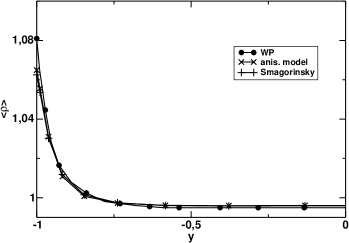
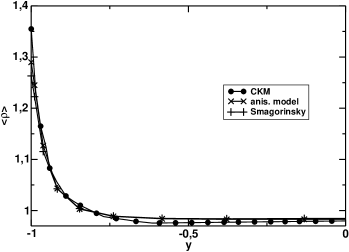
Figure 1: Mean density profiles at $Ma=0.7$ (Fig.1) and $Ma=1.5$ (Fig.1).

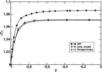
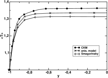
Figure 2: Mean temperature profiles at $Ma=0.7$ (Fig.2) and $Ma=1.5$ (Fig.2).

Figure 1 confirms the mean density values reported in Table 2. The excess in the density profiles at the channel center is related to the temperature values lower than the DNS ones far from the wall (see Figure 2). In spite of this, in Figure 2 the mean temperature profiles demonstrate the improvement due to the modeling of subgrid terms in the energy equations with the anisotropic model with respect to the Smagorinsky one, especially in the supersonic case. Figure 3 shows instead the mean velocity profiles. It is apparent that the anisotropic model approximates better the DNS results close to the wall.

Figure 4 shows the mean profile of the non-solenoidal term$\frac{\partial}{\partial y}<\nolinebreak v\nolinebreak>$ in the supersonic case. With the anisotropic model, the compression near the wall is underestimated, but the peak position is well captured, while this is not the case for the Smagorinsky model. At the center of the channel, while for the DNS a small dilatation is present, for the LES a small compression is probably necessary to compensate the excess of dilatation taking place in the buffer layer between the wall region and the logarithmic layers.

In figures 5-7, the root mean square values of the resolved velocity fluctuations are displayed. Figure 5 for the streamwise turbulence intensity shows that the Smagorinsky model presents different behavior depending on the Mach number. In the incompressible limit, the dissipative character of the Smagorinsky model leads to an overprediction of the streamwise turbulence intensity in the wall region, as often verified in other LES experiments (see for instance [33]). We recall that these quantities represent the resolved contributions only, so that their overestimation with respect to the DNS value is an undesired result. In the compressible simulations, instead, the Smagorinsky model predicts well the value of the peak but not the position. Moreover, the fluctuations are larger than those of the DNS far from the wall. On the other hand, the fluctuation peak is always well captured by the anisotropic model. Furthermore, while for $Ma=0.2$ the streamwise intensities are overpredicted by the anisotropic model in the center region, in the other tests they are well estimated.

The fluctuations of the velocity components normal to the wall (Figure 6) and spanwise (Figure 7) in the wall region are underestimated by both models with respect to the DNS values, although we recall that these are the resolved contribution only. For these components the difference between the Smagorinsky and the anisotropic model become less evident as the Mach number increases, but the anisotropic model always performs better. As it usually happens in LES experiments, lower values of the wall normal components obtained with the Smagorinsky model are associated to the overprediction of the streamwise fluctuations. In the centerline region, where the turbulence presents a more isotropic character, the anisotropic model tends to recover the Smagorinsky model results, especially at $Ma=0.2$.

In Figure 8 results for the total (modelled plus resolved) turbulent kinetic energy are displayed. For the Smagorinsky model, this corresponds to the resolved turbulent kinetic energy, since the isotropic part of the subgrid stresses is neglected. It can be observed that also for this quantity the DNS results are very well reproduced by the anisotropic model.

Since during the simulations a constant mass flow is imposed, the wall shear stress $\tau_{{\rm w}}$ can differ from the expected DNS value (see Table 2) and relevant differences affect also the wall normal turbulent shear stress (modeled + resolved) reported in Figure 9. Here, the stress is rescaled by the corresponding $u_{\tau}$ wall friction velocity obtained by each simulation. In spite of the application of the damping function, the Smagorinsky model does not present the correct trend at the wall and the shear stress is overestimated. This behaviour is probably the cause of the underprediction of the mean velocity profile in the wall region and of its difficulties in connecting properly the wall region to the the logarithmic layer. On the other hand, the anisotropic model is in quite good agreement with the DNS results for simulations at all Mach numbers.

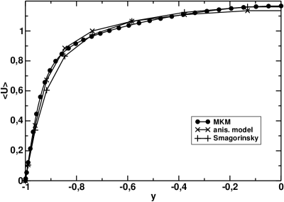
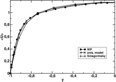
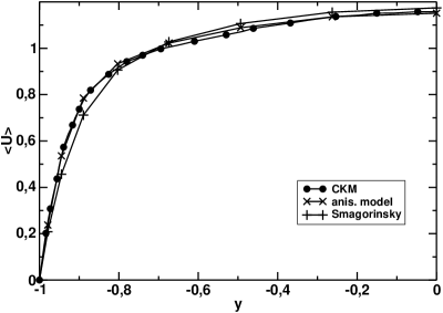
Figure 3: Mean streamwise velocity profiles at (a) $Ma=0.2,$ (b) $Ma=0.7$ and (c) $Ma=1.5.$

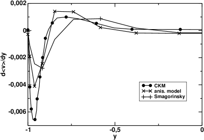
Figure 4: Mean dilatation profiles at $Ma=1.5.$

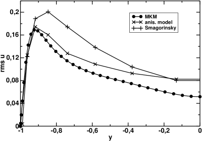
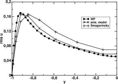
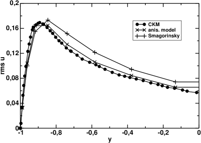
Figure 5: Root mean square profiles of the streamwise velocity component at (a) $Ma=0.2$, (b) $Ma=0.7$ and (c) $Ma=1.5$.

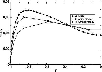
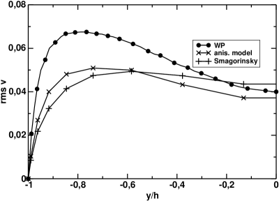
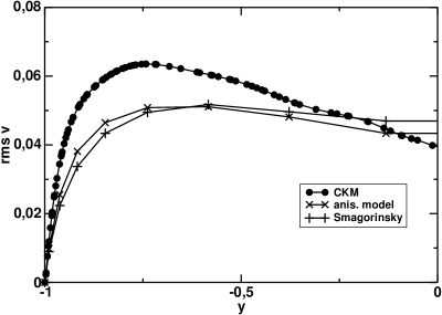
Figure 6: Root mean square profiles of the wall normal velocity component at (a) $Ma=0.2$, (b) $Ma=0.7$ and (c) $Ma=1.5$.

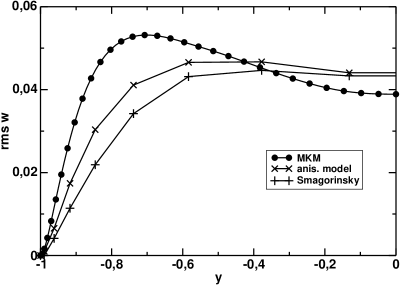
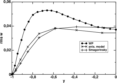
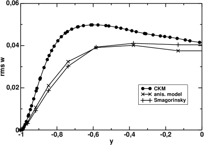
Figure 7: Root mean square profiles of the spanwise velocity components at (a) $Ma=0.2$, (b) $Ma=0.7$ and (c) $Ma=1.5$.

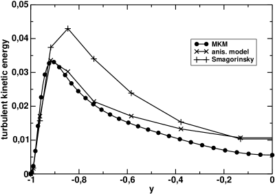
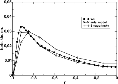
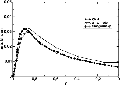
Figure 8: Total modelled+resolved turbulent kinetic energy at (a) $Ma=0.2$, (b) $Ma=0.7$ and (c) $Ma=1.5$.

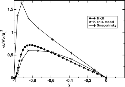
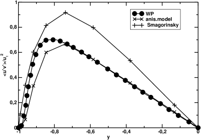
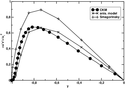
Figure 9: Total modelled+resolved turbulent wall normal shear stress at (a) $Ma=0.2$, (b) $Ma=0.7$ and (c) $Ma=1.5$. The stress is normalized by the corresponding $u_{\tau}$ wall friction velocity obtained by the simulation.

6 Conclusions and future perspectives

We have investigated the potential benefits resulting from the application of the anisotropic dynamic model [2] in the context of a high order DG model. This approach contrasts with other attempts at implementing LES in a DG framework, in which only Smagorinsky closures have been applied so far. Furthermore, the hierarchical nature of the DG finite element basis was exploited to implement the LES grid and test filters via projections on the finite dimensional subspaces that define the numerical approximation, along the lines of similar proposals in the VMS framework. A comparison with the DNS experiment results reported in [7], [37] and [51] has been carried out. The results of the comparison show a clear improvement in the prediction of several key features of the flow with respect to the Smagorinsky closure implemented in the same framework. The proposed approach appears to lead to significant improvements both in the low and high Mach number regimes. On this basis, we plan to investigate further extensions of this approach to flows in presence of gravity, with the goal of improving the turbulence models for applications to environmental stratified flows. Furthermore, the numerical framework that has been validated by the comparison reported in this paper will be employed for the assessment of the proposal presented in [36] for the extension of the eddy viscosity model to compressible flows.

References

- [1] A. Abbà, C. Cercignani, G. Picarella, and L. Valdettaro. A 3D turbulent boundary layer test for LES models. In Computational Fluid Dynamics 2000, 2001.
- [2] A. Abbà, C. Cercignani, and L. Valdettaro. Analysis of Subgrid Scale Models. Computer and Mathematics with Applications, 46:521–535, 2003.
- [3] D.N. Arnold, F. Brezzi, B. Cockburn, and L.D. Marini. Unified analysis of Discontinuous Galerkin methods for elliptic problems. SIAM Journal of Numerical Analysis, 39:1749–1779, 2002.
- [4] F. Bassi and S. Rebay. A High Order Accurate Discontinuous Finite Element Method for the Numerical Solution of the Compressible Navier-Stokes Equations. Journal of Computational Physics, 131:267–279, 1997.
- [5] P. Castillo, B. Cockburn, I. Perugia, and D. Schötzau. An a priori analysis of the Local Discontinuous Galerkin method for elliptic problems. SIAM Journal of Numerical Analysis, 38:1676–1706, 2000.
- [6] B. Cockburn and C. Shu. The Local Discontinuous Galerkin Method for Time-Dependent Convection-Diffusion Systems. SIAM Journal of Numerical Analysis, 35:2440–2463, 1998.
- [7] G.N. Coleman, J. Kim, and R.D. Moser. A numerical study of turbulent supersonic isothermal-wall channel flow. Journal of Fluid Mechanics, 305:159–183, 1995.
- [8] S. S. Collis. Discontinuous Galerkin methods for turbulence simulation. In Proceedings of the 2002 Center for Turbulence Research Summer Program, pages 155–167, 2002.
- [9] S. S. Collis and Y. Chang. The DG/VMS method for unified turbulence simulation. AIAA paper, 3124:24–27, 2002.
- [10] R. Cools. An Encyclopaedia of Cubature Formulas. Journal of Complexity, 19:445–453, 2003.
- [11] F.van der Bos, J.J.W. van der Vegt, and B.J. Geurts. A multi-scale formulation for compressible turbulent flows suitable for general Variational discretization techniques. Computer Methods in Applied Mechanics and Engineering, 196:2863–2875, 2007.
- [12] T.M. Eidson. Numerical simulation of turbulent Rayleigh-Bénard problem using subgrid modeling. Journal of Fluid Mechanics, 158:245–268, 1985.
- [13] G. Erlebacher, M.Y. Hussaini, C.G. Speziale, and T.A. Zang. Large Eddy Simulation of compressible turbulent flows. Journal of Fluid Mechanics, 238:155–185, 1992.
- [14] FEMilaro, a finite element toolbox. https://code.google.com/p/femilaro/. Available under GNU GPL v3.
- [15] F. Garcia, L. Bonaventura, M. Net, and J. Sánchez. Exponential versus IMEX high-order time integrators for thermal convection in rotating spherical shells. Journal of Computational Physics, 264:41–54, 2014.
- [16] E. Garnier, N. Adams, and P. Sagaut. Large Eddy Simulation for Compressible Flows. Springer Verlag, 2009.
- [17] M. Germano. Turbulence: the filtering approach. Journal of Fluid Mechanics, 238:325–336, 1992.
- [18] M. Germano, U. Piomelli, P. Moin, and W. H. Cabot. A Dynamic Subgrid-Scale Eddy Viscosity Model. Physics of Fluids, 3(7):1760–1765, 1991.
- [19] G. Gibertini, A. Abbà, F. Auteri, and M. Belan. Flow around two in-tandem flat plates: Measurements and computations comparison. In 5th International Conference on Vortex Flows and Vortex Models (ICVFM2010), 2010.
- [20] F.X. Giraldo and M. Restelli. A study of spectral element and discontinuous Galerkin methods for the Navier-Stokes equations in nonhydrostatic mesoscale atmospheric modeling: equation sets and test cases. Journal of Computational Physics, 227:3849–3877, 2008.
- [21] F.X. Giraldo, M. Restelli, and M. Läuter. Semi-implicit formulations of the Navier-Stokes equations: application to nonhydrostatic atmospheric modeling. SIAM Journal of Scientific Computing, 32:3394–3425, 2010.
- [22] T.J.R. Hughes, G.R. Feijoo, L. Mazzei, and J.B. Quincy. The Variational Multiscale method-a paradigm for computational mechanics. Computer Methods in Applied Mechanics and Engineering, 166:3–24, 1998.
- [23] T.J.R. Hughes, L. Mazzei, and K. Jansen. Large Eddy Simulation and the Variational Multiscale method. Computing and Visualization in Science, 3:47–59, 2000.
- [24] T.J.R. Hughes, L. Mazzei, A.A. Oberai, and A.A. Wray. The Multiscale formulation of Large Eddy Simulation: Decay of homogeneous isotropic turbulence. Physics of Fluids, 13:505–512, 2001.
- [25] T.J.R. Hughes, A.A. Oberai, and L. Mazzei. LargeEddy Simulation of turbulent channel flows by the Variational Multiscale method. Physics of Fluids, 13:1784–1799, 2001.
- [26] T.J.R. Hughes, G. Scovazzi, and L.P. Franca. Multiscale and stabilized methods. Wiley, 2004.
- [27] V. John and A. Kindl. Numerical studies of finite element Variational Multiscale Methods for turbulent flow simulations. Computer Methods in Applied Mechanics and Engineering, 199:841–852, 2010.
- [28] V. John and M. Roland. Simulations of the turbulent channel flow at with projection-based finite element Variational Multiscale Methods. International Journal of Numerical Methods in Fluids, 55:407–429, 2007.
- [29] D. Knight, G. Zhou, N. Okong’o, and V.Shukla. Compressible Large Eddy Simulation using unstructured grids. Technical Report 98-0535, American Institute of Aeronautics and Astronautics, 1998.
- [30] B. Koobus and C. Farhat. A Variational Multiscale method for the Large Eddy Simulation of compressible turbulent flows on unstructured meshes—-application to vortex shedding. Computer Methods in Applied Mechanics and Engineering, 193:1367–1383, 2004.
- [31] J. Lander and B.J. Hoskins. Believable scales and parameterizations in a spectral transform model. Monthly Weather Review, 125:292–303, 1997.
- [32] B. Landmann, M. Kessler, S. Wagner, and E. Krämer. A parallel, high-order discontinuous Galerkin code for laminar and turbulent flows. Computers & Fluids, 37:427–438, 2008.
- [33] E. Lenormand, P.Sagaut, and L. Ta Phuoc. Large Eddy Simulation of subsonic and supersonic channel flow at moderate Reynolds number. International Journal of Numerical Methods in Fluids, 32:369–406, 2000.
- [34] A. Maggioni. Formulazione DG-LES per flussi turbolenti comprimibili: modelli e validazione in un canale piano. Master’s thesis, School of Industrial Engineering, Politecnico di Milano, 2012.
- [35] M. Pino Martin, U. Piomelli, and G.V. Candler. Subgrid-Scale Models for Compressible Large-Eddy Simulations. Theoretical and Computational Fluid Dynamics, 13:361–376, 2000.
- [36] M.Germano, A. Abbà, R. Arina, and L. Bonaventura. On the extension of the eddy viscosity model to compressible flows. Physics of Fluids, 26(4):041702, 2014.
- [37] R.D. Moser, J. Kim, and N.N. Mansour. Direct numerical simulation of turbulent channel flow up to . Physics of Fluids, 11:943–945, 1999.
- [38] E.A. Munts, S.J. Hulshoff, and R. de Borst. A modal-based multiscale method for large eddy simulation. Journal of Computational Physics, 224:389–402, 2007.
- [39] M. Restelli and F.X. Giraldo. A conservative Discontinuous Galerkin semi-implicit formulation for the Navier-Stokes equations in nonhydrostatic mesoscale modeling. SIAM Journal of Scientific Computing, 31:2231–2257, 2009.
- [40] P. Sagaut. Large Eddy Simulation for Incompressible Flows: An Introduction. Springer Verlag, 2006.
- [41] H. Schlichting. Boundary-layer theory.7th edition. McGraw-Hill, 1979.
- [42] F.G. Schmitt. About Boussinesq’s turbulent viscosity hypothesis: historical remarks and a direct evaluation of its validity. Comptes Rendus Mécanique, 335:617–627, 2007.
- [43] J. C. Schulze, P. J. Schmid, and J. L. Sesterhenn. Exponential time integration using Krylov subspaces. International Journal of Numerical Methods in Fluids, 60:591–609, 2009.
- [44] A. Scotti, C. Meneveau, and D. Lilly. Generalized Smagorinsky Model for Anisotropic Grids. Physics of Fluids, 5(9):2306–2308, 1993.
- [45] K. Sengupta, F. Mashayek, and G.B. Jacobs. Large Eddy Simulation using a discontinuos Galerkin spectral method. In 45th AIAA Aerospace Sciences Meeting and Exhibit. AIAA, AIAA-2007-402 2007.
- [46] R.J. Spiteri and S.J. Ruuth. A New Class of Optimal High-Order Strong-Stability-Preserving Time Discretization Methods. SIAM Journal of Numerical Analysis, 40:469–491, 2002.
- [47] G. Tumolo, L. Bonaventura, and M. Restelli. A semi-implicit, semi-Lagrangian, p-adaptive Discontinuous Galerkin method for the shallow water equations. Journal of Computational Physics, 232:46 67, 2013.
- [48] A. Uranga, P.O. Persson, M. Drela, and J. Peraire. Implicit Large Eddy Simulation of transition to turbulence at low Reynolds numbers using a Discontinuous Galerkin method. International Journal for Numerical Methods in Engineering, 87:232–261, 2011.
- [49] F. van der Bos and B.J. Geurts. Computational error-analysis of a Discontinuous Galerkin discretization applied to large-eddy simulation of homogeneous turbulence. Computer Methods in Applied Mechanics and Engineering, 199:903–915, 2010.
- [50] B. Vreman, B.J. Geurts, and H. Kuerten. .subgrid-modeling in LES of compressible flow. Applied Scientific Research, 54:191–203, 1995.
- [51] L. Wei and A. Pollard. Direct numerical simulation of compressible turbulent channel flows using the Discontinuous Galerkin method. Computers and Fluids, 47:85–100, 2011.
- [52] K.S. Yang and J.H. Ferziger. Large-Eddy Simulation of turbulent obstacle flow using a dynamic subgrid-scale model. AIAA Journal, 31:1406–1413, 1993.
- [53] A. Yoshizawa. Statistical theory for compressible turbulent flows with the application to subgrid modeling. Physics of Fluids, 29:2152–2164, 1986.
- [54] Y. Zang, R.L. Street, and J.R. Koseff. A dynamic mixed subgrid-scale model and its application to turbulent recirculating flows. Physics of Fluids, 5:3186–3196, 1993.