Combined analysis of the decays $\tau^{-}\to K_{S}\pi^{-}\nu_{\tau}$ and $\tau^{-}\to K^{-}\eta\nu_{\tau}$

Abstract

In a combined study of the decay spectra of $\tau^{-}\to K_{S}\pi^{-}\nu_{\tau}$ and $\tau^{-}\to K^{-}\eta\nu_{\tau}$ decays within a dispersive representation of the required form factors, we illustrate how the $K^{*}(1410)$ resonance parameters, defined through the pole position in the complex plane, can be extracted with improved precision as compared to previous studies. While we obtain a substantial improvement in the mass, the uncertainty in the width is only slightly reduced, with the findings $M_{K^{*\prime}}=1304\pm 17\,$MeV and $\Gamma_{K^{*\prime}}=171\pm 62\,$MeV. Further constraints on the width could result from updated analyses of the $K\pi$ and/or $K\eta$ spectra using the full Belle-I data sample. Prospects for Belle-II are also discussed. As the $K^{-}\pi^{0}$ vector form factor enters the description of the decay $\tau^{-}\to K^{-}\eta\nu_{\tau}$, we are in a position to investigate isospin violations in its parameters like the form factor slopes. In this respect also making available the spectrum of the transition $\tau^{-}\to K^{-}\pi^{0}\nu_{\tau}$ would be extremely useful, as it would allow to study those isospin violations with much higher precision.

1 Introduction

Hadronic decays of the $\tau$ lepton constitute a distinguished set of processes to study the strong interactions in its non-perturbative regime under rather clean conditions Braaten:1991qm ; Braaten:1988hc ; Narison:1988ni ; Braaten:1988ea . This happens because the corresponding amplitudes can be factorised into a purely electroweak part corresponding to the decay of the $\tau$ lepton into a quark-antiquark pair and the associated $\tau$ neutrino, times the hadronization of the left-handed quark bilinear current under the action of QCD. The uncertainties of the first part are completely negligible with respect to those of the second one, which allows a direct access to the hadronic currents that has been exploited successfully for decades Pich:2013lsa .

The dominant strangeness-changing $\tau$ decays are into $K\pi$ meson systems and the corresponding observables have been measured with increasing precision at LEP aleph99 ; opal04 , BaBar Aubert:2007jh and Belle Epifanov:2007rf . We would like to note that the BaBar collaboration published their analysis for the $K^{-}\pi^{0}$ mode Aubert:2007jh , while Belle studied the $K_{S}\pi^{-}$ decay channel Epifanov:2007rf . Belle’s spectrum became publicly available but the published BaBar analysis only concerned the branching fraction while the corresponding spectrum has not been released yet. As a result, all dedicated studies of the $\tau^{-}\to(K\pi)^{-}\nu_{\tau}$ decays focused on the $K_{S}\pi^{-}$ system Jamin:2006tk ; Moussallam:2007qc ; Jamin:2008qg ; Boito:2008fq ; Boito:2010me ; Bernard:2013jxa . Consequently, even using data from semileptonic Kaon decays ($K\to\pi\ell\nu$, so-called $K_{\ell 3}$ decays) Boito:2010me ; Bernard:2013jxa , important information on isospin breaking effects in the low-energy expansion of the hadronic form factors could not be extracted. The quoted references succeeded in improving the determination of the $K^{*}(892)$ and $K^{*}(1410)$ resonance properties: their pole positions and relative weight, although the errors on the radial excitation were noticeably larger than in the $K^{*}(892)$ case.

The threshold for the decay $\tau^{-}\to K^{-}\eta\nu_{\tau}$ is above the region of $K^{*}(892)$-dominance which enhances its sensitivity to the properties of the heavier copy $K^{*}(1410)$. This observation was one of the motivations for the analysis of ref. Escribano:2013bca , where it was first shown that the considered decays were competitive to the $\tau^{-}\to(K\pi)^{-}\nu_{\tau}$ decays for the extraction of the $K^{*}(1410)$ meson parameters. This was made possible thanks to BaBar delAmoSanchez:2010pc and Belle Inami:2008ar data of the $K^{-}\eta$ spectrum which improved drastically the pioneering CLEO Bartelt:1996iv and ALEPH Buskulic:1996qs measurements.

The main purpose of this work is to illustrate the potential of a combined analysis of the decays $\tau^{-}\to(K\pi)^{-}\nu_{\tau}$ and $\tau^{-}\to K^{-}\eta\nu_{\tau}$ in the determination of the $K^{*}(1410)$ resonance properties. This study is presently limited by three facts: unfolding of detector effects has not been performed for the latter data, the associated errors of these are still relatively large and no measurement of the $K^{-}\pi^{0}$ spectrum has been published by the B-factories. We intend to demonstrate that an updated analysis of the $K_{S}\pi^{-}$ and/or $K^{-}\eta$ Belle spectrum including the whole Belle-I data sample could improve notably the knowledge of the $K^{*}(1410)$ pole position. Therefore, we hope that our paper strengths the case for a (re)analysis of the $(K\pi)^{-}$ and $K^{-}\eta$ spectra at the first generation B-factories including a larger data sample and also for devoted analyses in the forthcoming Belle-II experiment. Turning to the low-energy parameters, we emphasise the importance of (independent) measurements of the two $\tau^{-}\to(K\pi)^{-}\nu_{\tau}$ charge channels with the target of disentangling isospin violations in forthcoming studies.

While the $K\pi$-hadronization in the $\tau^{-}\to(K\pi)^{-}\nu_{\tau}$ decays is quite well understood, earlier analyses of $\tau^{-}\to K^{-}\eta\nu_{\tau}$ decays Pich:1987qq ; Braaten:1989zn ; Li:1996md were at odds with Belle data (also Kimura:2012 showed discrepancies) which motivated the claim in Belle’s paper Inami:2008ar that ‘further detailed studies of the physical dynamics in $\tau$ decays with $\eta$ mesons are required’, as also observed in ref. Actis:2010gg in a more general context. In ref. Escribano:2013bca , we showed that a simple Breit-Wigner parametrisation of the dominating vector form factor lead to a rather poor description of the data, while more elaborated approaches based on Chiral Perturbation Theory ($\chi PT$) Weinberg:1978kz ; Gasser:1983yg ; Gasser:1984gg including resonances as dynamical fields Ecker:1988te ; Ecker:1989yg and resumming final-state interactions (FSI) encoded in the chiral loop functions provided very good agreement with data. Since the $K^{-}\eta$ currents are presently modelled in TAUOLA Jadach:1990mz ; Jadach:1993hs (the standard Monte Carlo generator for $\tau$ lepton decays) relying on phase space, our form factors will enrich the Resonance Chiral Lagrangian-based currents Shekhovtsova:2012ra ; Nugent:2013hxa in the library (along these lines, the inclusion of the dispersive treatment for the $K\pi$ system is also in progress).

Our paper is organised as follows: in section 2, the differential decay width of the $\tau^{-}\to K_{S}\pi^{-}/K^{-}\eta\,\nu_{\tau}$ processes is written as a function of the contributing $K\pi$ vector and scalar form factors. The vector form factors will be described according to a dispersive representation along the lines of refs. Boito:2008fq ; Boito:2010me , while the scalar form factors are taken from refs. JOP00 ; JOP02 , thereby resumming FSI which is crucial to describe the considered decay spectra. Our previous analysis of the $\tau^{-}\to K^{-}\eta\nu_{\tau}$ decays Escribano:2013bca disfavoured strongly the use of Breit-Wigner functions, both from the theoretical and phenomenological perspective. In section 3, we describe our fits in detail and present the corresponding results for all parameters. It will be seen that we are able to improve the determination of the $K^{*}(1410)$ pole position. Furthermore, we discuss isospin violations on the slope parameters of the vector form factors and the prospects for improving them by analysing the full Belle-I data set or future measurements at Belle-II. Finally, we summarise our conclusions in section 4. A brief discussion of another so-called “exponential” parametrisation of the $K\pi$ vector form factor which was put forward in refs. Jamin:2006tk ; Jamin:2008qg is relegated to Appendix A.

2 Form factor representations

The differential decay width of the transition $\tau^{-}\to K_{S}\pi^{-}\nu_{\tau}$ as a function of the invariant mass of the two-meson system can be written as

$$\frac{{\rm d}\Gamma(\tau^{-}\to K_{S}\pi^{-}\nu_{\tau})}{{\rm d}\sqrt{s}} \,=\, \frac{G_{F}^{2}M_{\tau}^{3}}{96\pi^{3}s}S_{EW}\Big{|}V_{us}f_{+}^{K_{S}\pi^{-}}(0)\Big{|}^{2}\biggl{(}1-\frac{s}{M_{\tau}^{2}}\biggr{)}^{2}q_{K_{S}\pi^{-}}(s)$$ (1)

$$\times \biggl{\{}\left(1+\frac{2s}{M_{\tau}^{2}}\right)q_{K_{S}\pi^{-}}^{2}(s)\Big{|}\widetilde{f}_{+}^{K_{S}\pi^{-}}(s)\Big{|}^{2}+\frac{3\Delta_{K_{S}\pi^{-}}^{2}}{4s}\Big{|}\widetilde{f}_{0}^{K_{S}\pi^{-}}(s)\Big{|}^{2}\biggr{\}}\,,$$

where

$$q_{PQ}(s)\,=\,\frac{\sqrt{s^{2}-2s\Sigma_{PQ}+\Delta_{PQ}^{2}}}{2\sqrt{s}}\,,\quad\Sigma_{PQ}\,=\,m_{P}^{2}+m_{Q}^{2}\,,\quad\Delta_{PQ}\,=\,m_{P}^{2}-m_{Q}^{2}\,,$$ (2)

and

$$\widetilde{f}_{+,0}^{PQ}(s)\,\equiv\,\frac{f_{+,0}^{PQ}(s)}{f_{+,0}^{PQ}(0)}$$ (3)

are form factors normalised to unity at the origin. In this way, besides the global normalisation, all remaining uncertainties on the hadronization of the considered currents are encoded in the reduced form factors $\widetilde{f}_{+,0}^{PQ}(s)$. $S_{EW}=1.0201$ Erler:2002mv resums the short-distance electroweak corrections. Eq. (1) corresponds to the definitions of the vector, $f_{+}^{PQ}(s)$, and scalar, $f_{0}^{PQ}(s)$, form factors that separate the P- and S-wave contributions according to the conventions of ref. Gasser:1984ux . The corresponding formula for the $\tau^{-}\to K^{-}\eta\nu_{\tau}$ decays can be obtained by multiplying eq. (1) with the ratio between the corresponding SU(3) Clebsch-Gordan coefficients (three in this case) and replacing the $K_{S}$ and $\pi^{-}$ masses by those of the $K^{-}$ and $\eta$ mesons. A more detailed derivation of the differential distribution in the $K\eta$ case can be found in ref. Escribano:2013bca . Regarding the global normalisation, in the following we will employ $|V_{us}f_{+}^{K_{S}\pi^{-}}(0)|=0.2163(5)$ Antonelli:2010yf , from a global fit to $K_{\ell 3}$ data, and $|V_{us}f_{+}^{K^{-}\eta}(0)|=|V_{us}f_{+}^{K_{S}\pi^{-}}(0)|\cos\theta_{P}$, with $\theta_{P}=-(13.3\pm 1.0)^{\circ}$ Ambrosino:2006gk .

The required form factors cannot be computed analytically from first principles. Still, the symmetries of the underlying QCD Lagrangian are useful to determine their behaviour in specific limits, the chiral or low-energy limit and the high-energy behaviour, so that the model dependence is reduced to the interpolation between these known regimes. For our central fits, to be presented in the next section, we follow the dispersive representation of the vector form factors outlined in ref. Boito:2008fq , and briefly summarised below for the convenience of the reader. For the case of the $K_{S}\pi^{-}$ system, including two resonances, the $K^{*}=K^{*}(892)$ and the $K^{*\prime}=K^{*}(1410)$, the reduced vector form factor is taken to be of the form Boito:2008fq

$$\widetilde{f}_{+}^{K\pi}(s)\,=\,\frac{m_{K^{*}}^{2}-\kappa_{K^{*}}\,\widetilde{H}_{K\pi}(0)+\gamma s}{D(m_{K^{*}},\gamma_{K^{*}})}-\frac{\gamma s}{D(m_{K^{*\prime}},\gamma_{K^{*\prime}})}\,,$$ (4)

where

$$D(m_{n},\gamma_{n})\,=\,m_{n}^{2}-s-\kappa_{n}\widetilde{H}_{K\pi}(s)\,,$$ (5)

and

$$\kappa_{n}\,=\,\frac{192\pi}{\sigma_{K\pi}(m_{n}^{2})^{3}}\frac{\gamma_{n}}{m_{n}}\,.$$ (6)

The fit function for the vector form factor is expressed in terms of the unphysical “mass” and “width” parameters $m_{n}$ and $\gamma_{n}$. They are denoted by small letters, to distinguish them from the physical mass and width parameters $M_{n}$ and $\Gamma_{n}$, which will later be determined from the pole positions in the complex plane and are denoted by capital letters. The scalar one-loop integral function $\widetilde{H}_{K\pi}(s)$ is defined below eq. (3) of ref. Jamin:2006tk , however removing the factor $1/f_{\pi}^{2}$ which cancels if $\kappa_{n}$ is expressed in terms of the unphysical width $\gamma_{n}$. Finally, in eq. (6), the phase space function $\sigma_{K\pi}(s)$ is given by $\sigma_{K\pi}(s)=2q_{K\pi}(s)/\sqrt{s}$. Since the $K^{*}$ resonances that are produced through the $\tau$ decay are charged, and can decay or rescatter into both $K^{0}\pi^{-}$ as well as $K^{-}\pi^{0}$ channels, in the resonance propagators described by eqs. (4) to (6) we have chosen to employ the corresponding isospin average, that is

$$\widetilde{H}_{K\pi}(s)\,=\,\frac{2}{3}\,\widetilde{H}_{K^{0}\pi^{-}}(s)+\frac{1}{3}\,\widetilde{H}_{K^{-}\pi^{0}}(s)\,,$$ (7)

and analogously for $\sigma_{K\pi}(s)$, such that the resonance width contains both contributions. Little is known about a proper description of the width of the second vector resonance $K^{*\prime}$. The complicated $K^{*}\pi\sim K\pi\pi$ cuts may yield relevant effects which however necessitates a coupled-channel analysis like in refs. Moussallam:2007qc ; Bernard:2013jxa . This is beyond the scope of the present paper, in which for simplicity also for the second resonance only the two-meson cut is included. Similar remarks apply to a proper inclusion of the $K\eta$ and $K\eta^{\prime}$ channels into eq. (7) which would also require a coupled-channel analysis as was done for the corresponding scalar form factors in refs. JOP00 ; JOP02 .

Next, we further follow ref. Boito:2008fq in writing a three-times subtracted dispersive representation for the vector form factor,

$$\widetilde{f}_{+}^{K\pi}(s)\,=\,\exp\Biggl{[}\,\alpha_{1}\frac{s}{M_{\pi^{-}}^{2}}+\frac{1}{2}\alpha_{2}\frac{s^{2}}{M_{\pi^{-}}^{4}}+\frac{s^{3}}{\pi}\int\limits_{s_{K\pi}}^{s_{\rm cut}}{\rm d}s^{\prime}\frac{\delta_{1}^{K\pi}(s^{\prime})}{(s^{\prime})^{3}(s^{\prime}-s-i0)}\,\Biggr{]}\,,$$ (8)

where $s_{K\pi}=(M_{K}+M_{\pi})^{2}$ is the $K\pi$ threshold and the two subtraction constants $\alpha_{1}$ and $\alpha_{2}$ are related to the slope parameters appearing in the low-energy expansion of the form factor:

$$\widetilde{f}_{+}^{K\pi}(s)\,=\,1+\lambda_{+}^{{}^{\prime}}\frac{s}{M_{\pi^{-}}^{2}}+\frac{1}{2}\lambda_{+}^{{}^{\prime\prime}}\frac{s^{2}}{M_{\pi^{-}}^{4}}+\frac{1}{6}\lambda_{+}^{{}^{\prime\prime\prime}}\frac{s^{3}}{M_{\pi^{-}}^{6}}+\ldots\,.$$ (9)

Explicitly, the relations for the linear and quadratic slope parameters $\lambda_{+}^{{}^{\prime}}$ and $\lambda_{+}^{{}^{\prime\prime}}$ take the form:

$$\lambda_{+}^{{}^{\prime}}\,=\,\alpha_{1}\,,\qquad\lambda_{+}^{{}^{\prime\prime}}\,=\,\alpha_{2}+\alpha_{1}^{2}\,.$$ (10)

The incentive for employing a dispersive representation for the form factor is that in this way the influence of the less-well known higher energy region is suppressed. The associated error can be estimated by varying the cut-off $s_{\rm cut}$ in the dispersive integral. In order to obtain the required input phase $\delta_{1}^{K\pi}(s)$, like in Boito:2008fq we use the resonance propagator representation eq. (4) of the vector form factor. The phase can then be calculated from the relation

$$\tan\delta_{1}^{K\pi}(s)=\frac{{\rm Im}\widetilde{f}_{+}^{K\pi}(s)}{{\rm Re}\widetilde{f}_{+}^{K\pi}(s)}\,,$$ (11)

which completes our representation of the vector form factor $\widetilde{f}_{+}^{K\pi}(s)$.

The scalar form factors that are required for a complete description of the decay spectra according to eq. (1) will be taken from the coupled-channel dispersive representation of refs. JOP00 ; JOP02 . In particular, for the scalar $K\pi$ form factor, we employ the update presented in ref. JOP06 . For the scalar $K\eta$ form factor, the result of the three-channel analysis described in section 4.3 of JOP02 is used, choosing specifically the solution corresponding to fit (6.10) of ref. JOP00 . As a matter of principle, this is not fully consistent, since the employed $K\pi$ form factor was extracted from a two-channel analysis, only including the dominant $K\pi$ and $K\eta^{\prime}$ channels. But as our numerical analysis shows, anyway the influence of the scalar $K\eta$ form factor is insignificant so that this inconsistency can be tolerated.

3 Joint fits to $\tau^{-}\to K_{S}\pi^{-}\nu_{\tau}$ and $\tau^{-}\to K^{-}\eta\nu_{\tau}$ Belle data

The differential decay rate of eq. (1) is related to the distribution of the measured number of events by means of

$$\frac{{\rm d}N_{\rm events}}{{\rm d}\sqrt{s}}\,=\,\frac{{\rm d}\Gamma(\tau^{-}\to(PQ)^{-}\nu_{\tau})}{{\rm d}\sqrt{s}}\,\frac{N_{\rm events}}{\Gamma_{\tau}\bar{B}(\tau^{-}\to(PQ)^{-}\nu_{\tau})}\,\Delta\sqrt{s_{\rm bin}}\,,$$ (12)

where $N_{\rm events}$ is the total number of events measured for the considered process, $\Gamma_{\tau}$ is the inverse $\tau$ lifetime and $\Delta\sqrt{s_{\rm bin}}$ is the bin width. $\bar{B}(\tau^{-}\to(PQ)^{-}\nu_{\tau})\equiv\bar{B}_{PQ}$ is a normalisation constant that, for a perfect description of the spectrum, would equal the corresponding branching fraction.

For the $\tau^{-}\to K_{S}\pi^{-}\nu_{\tau}$ decays, an unfolded distribution measured by Belle is available Epifanov:2007rf . The corresponding number of events is $53113.21$ ($54157.59$ before unfolding) and the bin width $11.5\,$MeV. As discussed in the earlier analyses, the data points corresponding to bins $5$, $6$ and $7$ are difficult to bring into accord with the theoretical descriptions and have thus been excluded from the minimisation. The first point has not been included either, since the centre of the bin lies below the $K_{S}\pi^{-}$ production threshold. Following a suggestion from the experimentalists, as in the previous analyses we have furthermore excluded data corresponding to bin numbers larger than $90$.

On the other hand, the published $\tau^{-}\to K^{-}\eta\nu_{\tau}$ Belle data Inami:2008ar are only available still folded with detector effects. Lacking for a better alternative, we have assumed that the $K^{-}\eta$ unfolding function is reasonably estimated by the $K_{S}\pi^{-}$ one and we have extracted in this way pseudo-unfolded data that we employed in our analysis. The corresponding number of events turns out $1271.51$ for a bin width of $25$ MeV. In this case, we excluded the first three data points, which lie below the $K^{-}\eta$ production threshold, and discarded data above the $\tau$ mass.

The $\chi^{2}$ function minimised in our fits was chosen to be

$$\chi^{2}\,=\,\sum_{i,\;PQ=K_{S}\pi^{-},\,K^{-}\eta}{}^{{}^{\prime}}\hskip 25.60747pt\left(\frac{\mathcal{N}_{i}^{th}-\mathcal{N}_{i}^{exp}}{\sigma_{\mathcal{N}_{i}^{exp}}}\right)^{2}+\sum_{PQ=K_{S}\pi^{-},\,K^{-}\eta}\left(\frac{\bar{B}_{PQ}^{th}-B_{PQ}^{exp}}{\sigma_{B_{PQ}}^{exp}}\right)^{2}\,,$$ (13)

where $\mathcal{N}_{i}^{exp}$ and $\sigma_{\mathcal{N}_{i}^{exp}}$ are, respectively, the experimental number of events and the corresponding uncertainties in the $i$-th bin. The prime in the summation indicates that the points specified above have been excluded. Therefore, the number of fitted data points is $86$ ($28$) for the $K_{S}\pi^{-}$ ($K^{-}\eta$) spectrum, together with the respective branching fractions: hence $116$ data points in total. While it is possible to obtain stable fits without using the $K_{S}\pi^{-}$ branching fraction as a data point, this is not the case for the $K^{-}\eta$ channel. This is due to the fact that there are strong correlations between the branching ratio and the slope parameters of the vector form factor. While in the $K_{S}\pi^{-}$ case sufficiently many data points with small enough errors are available to determine all fit quantities from the spectrum, for the $K^{-}\eta$ decay mode this was not possible. As a consistency check, we will be comparing the fitted values of the respective branching ratios to the corresponding results obtained by directly integrating the spectrum in all our fits.

The fitted parameters within the dispersive representation of the form factors of eq. (8) then include:

• the respective branching fractions $\bar{B}_{K\pi}$ and $\bar{B}_{K\eta}$. For consistency, as our inputs in eq. (13) we employ the results obtained by Belle in correspondence with the employed decay distribution data: $(0.404\pm 0.013)\%$ Epifanov:2007rf as well as $(1.58\pm 0.10)\times 10^{-4}$ Inami:2008ar , respectively. This may be compared to the averages by the Particle Data Group, $(0.420\pm 0.020)\%$ and $(1.52\pm 0.08)\times 10^{-4}$ Beringer:1900zz and Heavy Flavour Averaging Group values Amhis:2012bh , $(0.410\pm 0.009)\%$ and $(1.53\pm 0.08)\times 10^{-4}$. The recent update by Belle Ryu:2014vpc including a 669 fb^-1 data sample was found to be $(0.416\pm 0.008)\%$ for the former decay mode.

• The slope parameters: $\lambda^{\prime(\prime)}_{K\pi}$ and $\lambda^{\prime(\prime)}_{K\eta}$. As was noted in ref. Escribano:2013bca , while the former ones correspond to the $K_{S}\pi^{-}$ channel, the latter ones are related to the $K^{-}\pi^{0}$ system. Therefore, small differences in these parameters due to isospin violations are expected, and in the most general fit we allow for independent parameters in the two channels. As consistency checks of our procedure, we have also considered some fits assuming $\lambda^{\prime}_{K\eta}=\lambda^{\prime}_{K\pi}$. The findings of ref. Boito:2008fq , $\lambda^{\prime}_{K\pi}=(24.66\pm 0.77)\times 10^{-3}$ and $\lambda^{\prime\prime}_{K\pi}=(11.99\pm 0.20)\times 10^{-4}$, should serve as a reference point for our present study, where however $\bar{B}_{K\pi}$ was fixed to the average $(0.418\pm 0.011)\%$ at that time.

• The pole parameters of the $K^{*}(892)$ and $K^{*}(1410)$ resonances. The masses and widths of these resonances are extracted from the complex pole position $s_{R}$ according to $\sqrt{s_{R}}=M_{R}-\frac{i}{2}\Gamma_{R}$ Escribano:2002iv . For the lowest-lying resonance our results for the pole mass and width should be compatible with $(892.0\pm 0.2)\,$MeV and $(46.2\pm 0.4)\,$MeV Boito:2010me , respectively, where the quoted uncertainties are only statistical. We expect that the extraction of the $K^{*}(1410)$ pole position should benefit from our present combined fit for which $(1273\pm 75)\,$MeV and $(185\pm 74)\,$MeV were obtained in ref. Boito:2008fq when the uncertainties are symmetrised.

• The relative weight $\gamma$ of the two resonances. In our isospin-symmetric way (4) of parametrising the resonance propagators in the form factor description, $\gamma$ should be the same for the $K_{S}\pi^{-}$ and $K^{-}\eta$ channels, which we shall assume for our central fit. Still, we have also tried to fit them independently, as differences might indicate inelastic or coupled-channel effects. As is seen below, our various fit results do not show a sizeable preference for this possibility which supports our choice $\gamma_{K\eta}=\gamma_{K\pi}$. Our findings may be compared to the value $\gamma=-0.039\pm 0.020$ of Boito:2008fq indicating the influence of including the $\tau^{-}\to K^{-}\eta\nu_{\tau}$ mode into our analysis.

In the fits we have furthermore employed the following numerical inputs: $M_{\tau}=1776.82\,$MeV, $\Gamma_{\tau}=2.265\times 10^{-12}\,$GeV and $G_{F}=1.16637(1)\times 10^{-5}\,$GeV^-2 Beringer:1900zz . Pseudoscalar meson masses were also taken according to their PDG values Beringer:1900zz . Finally, the next-to-leading order $\chi PT$ low-energy constants and the chiral logarithms depend on an arbitrary renormalisation scale $\mu$ (these dependencies cancel one another), which we have fixed to the physical mass scale of the problem, $M_{K^{*}}=892\,$MeV.

In Table 1, we display our results using slightly different settings, though in all of them eq. (11) is employed to obtain the input phaseshift for the dispersion relation (8) and $s_{\rm cut}$ is fixed to $4\,$GeV² (the uncertainty associated to its variation is discussed later on): our reference fit (second column) corresponds to fixing $\gamma_{K\pi}=\gamma_{K\eta}$, fit A (third column) assumes $\lambda^{\prime}_{K\pi}=\lambda^{\prime}_{K\eta}$, fit B (fourth column) is the result of letting all parameters float independently and finally, fit C (fifth column) enforces both restrictions $\gamma_{K\pi}=\gamma_{K\eta}$ and $\lambda^{\prime}_{K\pi}=\lambda^{\prime}_{K\eta}$. It is seen that our approach is rather stable against these variations, as the $\chi^{2}/$n.d.f. remains basically the same for the different scenarios. Also the values of the fitted parameters are always compatible across all fits. The largest modification is observed in fit A, where we fix $\lambda^{\prime}_{K\pi}=\lambda^{\prime}_{K\eta}$, but allow for independent resonance mixing parameters $\gamma$. This is partly expected since in the reference fit the former equality on the slope parameters is only fulfilled at the $2\sigma$ level. Letting all parameters float in fit B yields results which are nicely compatible with the reference fit, though for some parameters resulting in slightly larger uncertainties. Finally, enforcing both, the linear slopes as well as the mixing parameters to be equal also results in a compatible fit where now the largest shift by about $2\sigma$ is found in $\lambda^{{}^{\prime\prime}}_{K\eta}$.

Fitted value	Reference Fit	Fit A	Fit B	Fit C
$\bar{B}_{K\pi}(\%)$	$0.404\pm 0.012$	$0.400\pm 0.012$	$0.404\pm 0.012$	$0.397\pm 0.012$
$(B_{K\pi}^{th})(\%)$	$(0.402)$	$(0.394)$	$(0.400)$	$(0.394)$
$M_{K^{*}}$	$892.03\pm 0.19$	$892.04\pm 0.19$	$892.03\pm 0.19$	$892.07\pm 0.19$
$\Gamma_{K^{*}}$	$46.18\pm 0.42$	$46.11\pm 0.42$	$46.15\pm 0.42$	$46.13\pm 0.42$
$M_{K^{*\prime}}$	$1305^{+15}_{-18}$	$1308^{+16}_{-19}$	$1305^{+15}_{-18}$	$1310^{+14}_{-17}$
$\Gamma_{K^{*\prime}}$	$168^{+52}_{-44}$	$212^{+66}_{-54}$	$174^{+58}_{-47}$	$184^{+56}_{-46}$
$\gamma_{K\pi}\times 10^{2}$	$=\gamma_{K\eta}$	$-3.6^{+1.1}_{-1.5}$	$-3.3^{+1.0}_{-1.3}$	$=\gamma_{K\eta}$
$\lambda^{\prime}_{K\pi}\times 10^{3}$	$23.9\pm 0.7$	$23.6\pm 0.7$	$23.8\pm 0.7$	$23.6\pm 0.7$
$\lambda^{\prime\prime}_{K\pi}\times 10^{4}$	$11.8\pm 0.2$	$11.7\pm 0.2$	$11.7\pm 0.2$	$11.6\pm 0.2$
$\bar{B}_{K\eta}\times 10^{4}$	$1.58\pm 0.10$	$1.62\pm 0.10$	$1.57\pm 0.10$	$1.66\pm 0.09$
$(B_{K\eta}^{th})\times 10^{4}$	$(1.45)$	$(1.51)$	$(1.44)$	$(1.58)$
$\gamma_{K\eta}\times 10^{2}$	$-3.4^{+1.0}_{-1.3}$	$-5.4^{+1.8}_{-2.6}$	$-3.9^{+1.4}_{-2.1}$	$-3.7^{+1.0}_{-1.4}$
$\lambda^{\prime}_{K\eta}\times 10^{3}$	$20.9\pm 1.5$	$=\lambda^{\prime}_{K\pi}$	$21.2\pm 1.7$	$=\lambda^{\prime}_{K\pi}$
$\lambda^{\prime\prime}_{K\eta}\times 10^{4}$	$11.1\pm 0.4$	$11.7\pm 0.2$	$11.1\pm 0.4$	$11.8\pm 0.2$
$\chi^{2}/$n.d.f.	$108.1/105\sim 1.03$	$109.9/105\sim 1.05$	$107.8/104\sim 1.04$	$111.9/106\sim 1.06$

Table 1: Fit results for different choices regarding linear slopes and resonance mixing parameters at $s_{\rm cut}=4\,$GeV². See the main text for further details. Dimensionful parameters are given in MeV. As a consistency check, for each of the fits we provide (in brackets) the value of the respective branching fractions obtained by integrating eq. (1).

The theoretical uncertainty associated to the choice of $s_{\rm cut}$ is probed through the fits presented in Table 2 where, for the setting of our reference fit discussed previously, the values $3.24\,$GeV² (second column), $4\,$GeV² (third column), $9\,$GeV² (fourth column) and the $s_{\rm cut}\to\infty$ limit (last column) are used ($s_{\rm cut}=4\,$GeV² corresponds to our reference fit in the second column of Table 1 and is repeated here for ease of comparison). The dependence of the fitted parameters on the integral cut-off is similar to what was found in previous works (see, for instance refs. Boito:2008fq ; Boito:2010me ) and allows to estimate the corresponding systematic error. In order to corroborate our fits, we performed additional tests. We have also run fits considering two and four subtraction constants in order to test the stability of our results with respect to this choice. As in the previous analyses Boito:2008fq ; Boito:2010me of the $\tau^{-}\to K_{S}\pi^{-}\nu_{\tau}$ spectrum, the changes in the results are well within our uncertainties. It is furthermore confirmed that regarding final uncertainties three subtractions appears to be an optimal choice. This may, however, change if the representation of the higher-energy region is improved, for example through a coupled-channel analysis, such that this region requires less suppression. As a second test, we have employed a variant of the form factor Ansatz (4) in which the real part of the loop function $\widetilde{H}_{K\pi}(s)$ is not resummed into the propagator denominator, but into an exponential, as was for example suggested in refs. Jamin:2006tk ; Jamin:2008qg for the description of $\tau\to K\pi\nu_{\tau}$ decays. This type of Ansatz is further discussed in Appendix A where also direct fits of the corresponding form factors are described. Our test here, however, consists in extracting the corresponding phase from this type of form factor according to eq. (11) and plugging the respective phase into the dispersion relation (8). It is found that the corresponding fits are almost identical to the ones described before, providing additional faith on the robustness of the extracted parameters.

	$3.24$	$4$	$9$	$\infty$
$\bar{B}_{K\pi}(\%)$	$0.402\pm 0.013$	$0.404\pm 0.012$	$0.405\pm 0.012$	$0.405\pm 0.012$
$(B_{K\pi}^{th})(\%)$	$(0.399)$	$(0.402)$	$(0.403)$	$(0.403)$
$M_{K^{*}}$	$892.01\pm 0.19$	$892.03\pm 0.19$	$892.05\pm 0.19$	$892.05\pm 0.19$
$\Gamma_{K^{*}}$	$46.04\pm 0.43$	$46.18\pm 0.42$	$46.27\pm 0.42$	$46.27\pm 0.41$
$M_{K^{*\prime}}$	$1301^{+17}_{-22}$	$1305^{+15}_{-18}$	$1306^{+14}_{-17}$	$1306^{+14}_{-17}$
$\Gamma_{K^{*\prime}}$	$207^{+73}_{-58}$	$168^{+52}_{-44}$	$155^{+48}_{-41}$	$155^{+47}_{-40}$
$\gamma_{K\pi}$	$=\gamma_{K\eta}$	$=\gamma_{K\eta}$	$=\gamma_{K\eta}$	$=\gamma_{K\eta}$
$\lambda^{\prime}_{K\pi}\times 10^{3}$	$23.3\pm 0.8$	$23.9\pm 0.7$	$24.3\pm 0.7$	$24.3\pm 0.7$
$\lambda^{\prime\prime}_{K\pi}\times 10^{4}$	$11.8\pm 0.2$	$11.8\pm 0.2$	$11.7\pm 0.2$	$11.7\pm 0.2$
$\bar{B}_{K\eta}\times 10^{4}$	$1.57\pm 0.10$	$1.58\pm 0.10$	$1.58\pm 0.10$	$1.58\pm 0.10$
$(B_{K\eta}^{th})\times 10^{4}$	$(1.43)$	$(1.45)$	$(1.46)$	$(1.46)$
$\gamma_{K\eta}\times 10^{2}$	$-4.0^{+1.3}_{-1.9}$	$-3.4^{+1.0}_{-1.3}$	$-3.2^{+0.9}_{-1.1}$	$-3.2^{+0.9}_{-1.1}$
$\lambda^{\prime}_{K\eta}\times 10^{3}$	$18.6\pm 1.7$	$20.9\pm 1.5$	$22.1\pm 1.4$	$22.1\pm 1.4$
$\lambda^{\prime\prime}_{K\eta}\times 10^{4}$	$10.8\pm 0.3$	$11.1\pm 0.4$	$11.2\pm 0.4$	$11.2\pm 0.4$
$\chi^{2}/$n.d.f.	$105.8/105$	$108.1/105$	$111.0/105$	$111.1/105$

Table 2: Reference fit results obtained for different values of $s_{\rm cut}$ in the dispersive integral are displayed. Dimensionful parameters are given in MeV. As a consistency check, for each of the fits we give (in brackets) the value of the respective branching ratios obtained integrating eq. (1).

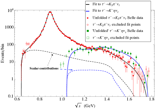
Figure 1: Belle $\tau^{-}\to K_{S}\pi^{-}\nu_{\tau}$ (red solid circles) Epifanov:2007rf and $\tau^{-}\to K^{-}\eta\nu_{\tau}$ (green solid squares) Inami:2008ar measurements as compared to our best fit results (solid black and blue lines, respectively) obtained in combined fits to both data sets, as presented in eq. (3). Empty circles (squares) correspond to data points which have not been included in the analysis. The small scalar contributions have been represented by black and blue dashed lines showing that while the former plays a role for the $K\pi$ spectrum close to threshold, the latter is irrelevant for the $K\eta$ distribution.

For presenting our final results, we have added to the statistical fit error a systematic uncertainty due to the variation of $s_{\rm cut}$. To this end, we have taken the largest variation of central values while varying $s_{\rm cut}$ (which is always found at $s_{\rm cut}=3.24\,$GeV²) and have added this variation in quadrature to the statistical uncertainty. We then obtain

$$\bar{B}_{K\pi}\,=\,\left(0.404\pm 0.012\right)\%\,,\quad M_{K^{*}}\,=\,892.03\pm 0.19\,,\quad\Gamma_{K^{*}}\,=\,46.18\pm 0.44\,,$$

$$M_{K^{*\prime}}\,=\,1305^{+16}_{-18}\,,\quad\Gamma_{K^{*\prime}}\,=\,168^{+65}_{-59}\,,\quad\gamma_{K\pi}=\gamma_{K\eta}=\left(-3.4^{+1.2}_{-1.4}\right)\cdot 10^{-2}\,,$$

$$\lambda^{\prime}_{K\pi}\,=\,\left(23.9\pm 0.9\right)\cdot 10^{-3}\,,\quad\lambda^{\prime\prime}_{K\pi}\,=\,\left(11.8\pm 0.2\right)\cdot 10^{-4}\,,\quad\bar{B}_{K\eta}\,=\,\left(1.58\pm 0.10\right)\cdot 10^{-4}\,,$$

$$\lambda^{\prime}_{K\eta}\,=\,\left(20.9\pm 2.7\right)\cdot 10^{-3}\,,\quad\lambda^{\prime\prime}_{K\eta}\,=\,\left(11.1\pm 0.5\right)\cdot 10^{-4}\,,$$ (14)

were like before all dimensionful quantities are given in MeV. Our final fit results are compared to the measured Belle $\tau^{-}\to K_{S}\pi^{-}\nu_{\tau}$ and $\tau^{-}\to K^{-}\eta\nu_{\tau}$ distributions Epifanov:2007rf ; Inami:2008ar in Figure 1. Satisfactory agreement with the experimental data, in accord with the observed $\chi^{2}$/n.d.f. of order one, is seen for all data points. The $K\pi$ spectrum is dominated by the contribution of the $K^{*}(892)$ resonance, whose peak is neatly visible. The scalar form factor contribution, although small in most of the phase space, is important to describe the data immediately above threshold. There is no such clear peak structure for the $K\eta$ channel as a consequence of the interplay between both $K^{*}$ resonances. The corresponding scalar form factor in this case is numerically insignificant.

The correlation coefficients corresponding to our reference fit with $s_{\rm cut}=4$ GeV² can be read from Table 3. As anticipated, there is a large correlation between the set $\{\bar{B}_{K\pi},\,\lambda^{\prime}_{K\pi},\,\lambda^{{}^{\prime\prime}}_{K\pi}\}$ which enables stable fits removing one of these parameters (the fit then becomes somewhat less restrictive, though). Despite the correlation between $\lambda^{\prime}_{K\eta}$ and $\lambda^{{}^{\prime\prime}}_{K\eta}$ also being nearly maximal, these parameters are less correlated with $\bar{B}_{K\eta}$, implying that all three are needed to reach convergence in the minimisation. For this reason we prefer to keep $\bar{B}_{K\eta}$ as a data point in the joint analysis. Finally, we note a large correlation between the parameters $\gamma_{K\pi}=\gamma_{K\eta}$ and $\Gamma_{K^{*\prime}}$ which seems to be enhancing the corresponding errors (this effect may in part be due to the three subtractions employed, which decrease the sensitivity to the higher-energy region). In the fits where $\gamma_{K\pi}=\gamma_{K\eta}$ is not enforced, their correlation coefficient is $\approx 0.67$. This suggests that with more precise data in the future it might be possible to resolve the current degeneracy between both.

	$\bar{B}_{K\pi}$	$M_{K^{*}}$	$\Gamma_{K^{*}}$	$M_{K^{*\prime}}$	$\Gamma_{K^{*\prime}}$	$\lambda^{\prime}_{K\pi}$	$\lambda^{\prime\prime}_{K\pi}$	$\bar{B}_{K\eta}$	$\gamma_{K\eta}=\gamma_{K\pi}$	$\lambda^{\prime}_{K\eta}$	$\lambda^{\prime\prime}_{K\eta}$
$M_{K^{*}}$	$-0.163$	$1$
$\Gamma_{K^{*}}$	$0.028$	$-0.060$	$1$
$M_{K^{*\prime}}$	$-0.063$	$-0.104$	$-0.142$	$1$
$\Gamma_{K^{*\prime}}$	$0.126$	$0.130$	$0.292$	$-0.556$	$1$
$\lambda^{\prime}_{K\pi}$	$0.800$	$-0.100$	$0.457$	$-0.244$	$0.432$	$1$
$\lambda^{\prime\prime}_{K\pi}$	$0.928$	$-0.215$	$0.328$	$-0.166$	$0.304$	$0.942$	$1$
$\bar{B}_{K\eta}$	$-0.003$	$-0.005$	$-0.010$	$0.003$	$-0.001$	$-0.015$	$-0.009$	$1$
$\gamma_{K\eta}=\gamma_{K\pi}$	$-0.155$	$-0.173$	$-0.378$	$0.498$	$-0.878$	$-0.565$	$-0.373$	$0.019$	$1$
$\lambda^{\prime}_{K\eta}$	$0.058$	$0.028$	$0.117$	$0.050$	$0.337$	$0.182$	$0.128$	$0.434$	$-0.340$	$1$
$\lambda^{\prime\prime}_{K\eta}$	$0.035$	$-0.017$	$0.037$	$0.106$	$0.218$	$0.080$	$0.064$	$0.561$	$-0.174$	$0.971$	$1$

Table 3: Correlation coefficients corresponding to our reference fit with $s_{\rm cut}=4$ GeV², second column of Table 1. In the fits where $\gamma_{K\pi}=\gamma_{K\eta}$ is not enforced, their correlation coefficient turns out to be $\approx 0.67$.

Several comments regarding our final results of eq. (3) and the reference fit of Table 1 are in order:

• Concerning the branching fractions, we observe that in the $K_{S}\pi^{-}$ channel our fit value $\bar{B}_{K\pi}$, which is mainly driven by the explicit input, and the result when integrating the fitted spectrum $B_{K\pi}^{th}$, are in very good agreement, pointing to a satisfactory description of the experimental data. On the other hand, for the $K\eta$ case, one notes a trend that the integrated branching fraction $B_{K\eta}^{th}$ turns out about $10\%$ smaller than the fit result $\bar{B}_{K\eta}$, which points to slight deficiencies in the theoretical representation of this spectrum. This issue should be investigated further in the future with more precise data.

• The $K_{S}\pi^{-}$ slope parameters are well compatible with previous analogous analysis Boito:2008fq ; Boito:2010me . For the corresponding $K^{-}\eta$ slopes, we obtain somewhat smaller values, which are, however, compatible with the crude estimates in Ref. Escribano:2013bca . The fact that the $K^{-}\eta$ slopes are about $2\sigma$ lower than the $K_{S}\pi^{-}$ slopes could be an indication of isospin violations, or could be a purely statistical effect. (Or a mixture of both.) To tackle this question and make further progress to disentangle isospin violations in the $K\pi$ form factor slopes, it is indispensable to study the related distribution for the $\tau^{-}\to K^{-}\pi^{0}\nu_{\tau}$ decay, and the experimental groups should make every effort to also publish the corresponding spectrum for this process.

• The pole parameters of the $K^{*}(892)$ resonance are in nice accord with previous values Boito:2008fq ; Boito:2010me and have similar statistical fit uncertainties which is to be expected as these parameters are driven by the data of the $\tau^{-}\to K_{S}\pi^{-}\nu_{\tau}$ decay, which was the process analysed previously. Regarding the parameters of the $K^{*}(1410)$ resonance, adding the $\tau^{-}\to K^{-}\eta\nu_{\tau}$ spectral data into the fit results in a substantial improvement in the determination of the mass, while only a slight improvement in the width is observed. Part of the large uncertainty in the width of the second $K^{*}$ resonance can be traced back to the strong fit correlation with the mixing parameter $\gamma$, which is also not very well determined. Future data of either $\tau^{-}\to(K\pi)^{-}\nu_{\tau}$ or $\tau^{-}\to K^{-}\eta\nu_{\tau}$ hadronic invariant mass distributions should enable a more precise evaluation. Prospects updating the Belle-I analyses with the complete data sample or studying Belle-II data are discussed next.

In Table 4, we have simulated the impact of future data on our fitted parameters. For this purpose we have kept the same central values of the data points and reduced the errors according to the expected increase in luminosity. Specifically, we have used that the $K_{S}\pi^{-}$ ($K^{-}\eta$) Belle analysis employed $351$ ($490$) fb^-1 for a complete data sample of $1000$ fb^-1 accumulated at Belle-I for general purpose studies (we have assumed the same resolution and efficiencies as in the published analyses following a suggestion from the Collaboration). Similarly, we have also compared our current results, eq. (3), to the prospects for Belle-II at the end of its data taking, with $50$ ab^-1 neglecting again possible improvements in the detector response and data analysis. In the different columns of Table 4, we recall our results, eq. (3), and compare them, in turn, to the cases where both decay modes are reanalysed using the whole Belle-I data sample, the same when only one of the analysis is updated and analogously for Belle-II.

	Current	Belle-I	Belle-I $K\pi$	Belle-I $K\eta$	Belle-II	Belle-II $K\pi$	Belle-II $K\eta$
$\bar{B}_{K\pi}(\%)$	$0.404\pm 0.012$	$\pm 0.005$	$\pm 0.005$	$\pm 0.012$	†($0.001$)	†($0.001$)	$\pm 0.012$
$M_{K^{*}}$	$892.03\pm 0.19$	$\pm 0.09$	$\pm 0.09$	$\pm 0.19$	†($0.02$)	†($0.02$)	$\pm 0.19$
$\Gamma_{K^{*}}$	$46.18\pm 0.44$	$\pm 0.20$	$\pm 0.20$	$\pm 0.44$	†($0.02$)	†($0.03$)	$\pm 0.42$
$M_{K^{*\prime}}$	$1304\pm 17$	†($7$)	†($9$)	†($8$)	†($1$)	†($1$)	†($1$)
$\Gamma_{K^{*\prime}}$	$168\pm 62$	†($19$)	†($24$)	†($25$)	†($3$)	†($4$)	†($11$)
$\lambda^{\prime}_{K\pi}\times 10^{3}$	$23.9\pm 0.9$	†($0.3$)	†($0.3$)	$\pm 0.8$	†($0.04$)	†($0.04$)	$\pm 0.8$
$\lambda^{\prime\prime}_{K\pi}\times 10^{4}$	$11.8\pm 0.2$	$\pm 0.07$	$\pm 0.07$	$\pm 0.2$	†($0.01$)	†($0.01$)	$\pm 0.2$
$\bar{B}_{K\eta}\times 10^{4}$	$1.58\pm 0.10$	$\pm 0.05$	$\pm 0.10$	$\pm 0.05$	†($0.01$)	$\pm 0.10$	†($0.01$)
$\gamma_{K\eta}(=\gamma_{K\pi})\times 10^{2}$	$-3.3\pm 1.3$	†($0.3$)	†($0.3$)	†($0.4$)	†($0.04$)	†($0.04$)	∘($0.3$)
$\lambda^{\prime}_{K\eta}\times 10^{3}$	$20.9\pm 2.7$	†($0.7$)	$\pm 2.7$	†($0.8$)	†($0.10$)	$\pm 2.7$	∘($0.4$)
$\lambda^{\prime\prime}_{K\eta}\times 10^{4}$	$11.1\pm 0.5$	†($0.2$)	$\pm 0.5$	†($0.2$)	†($0.02$)	$\pm 0.5$	†($0.06$)

Table 4: The errors of our final results (3) are compared, in turn, to those achievable by analysing the complete Belle-I data sample, and updating only the $K_{S}\pi^{-}$ or $K^{-}\eta$ analyses. The last three columns show the potential of fitting all data collected by Belle-II and the same only for $K_{S}\pi^{-}$ or for $K^{-}\eta$ (assuming the other mode has not been updated to include the complete Belle-I data sample). Current Belle $K_{S}\pi^{-}$ ($K^{-}\eta$) data correspond to $351$ ($490$) fb^-1 for a complete data set of $\sim 1000$ fb${}^{-1}=1$ ab^-1. Expectations for Belle-II correspond to 50 ab^-1. All errors include both statistical and systematic uncertainties. ^† means that statistical errors (in brackets) will become negligible, while ^∘ signals a tension with the current reference best fit values. We thank Denis Epifanov for conversations on these figures and on expected performance of Belle-II at the detector and analysis levels. All errors have been symmetrised for simplicity.

The majority of the expected errors for Belle-II will make completely negligible the statistical error with respect to the theoretical uncertainties, which then will most likely demand more elaborated approaches than those considered here. This would also happen in the case of the $K^{*}(1410)$ parameters with any updated Belle-I study. The impact of $\tau^{-}\to K^{-}\pi^{0}\nu_{\tau}$ on the $K^{*}(892)$ and $K^{*}(1410)$ meson parameters can be estimated by means of the $\tau^{-}\to K_{S}\pi^{-}\nu_{\tau}$ simulation. Such a measurement will be more significant in the determination of the $K^{-}\eta$ slope parameters than an updated study of this latter decay mode. In passing, we also mention that Belle-II statistics could be able to pinpoint possible inconsistencies between $\tau^{-}\to(K\pi)^{-}\nu_{\tau}$ and $\tau^{-}\to K^{-}\eta\nu_{\tau}$ data.

4 Conclusions

Hadronic decays of the $\tau$ lepton remain to be an advantageous tool for the investigation of the hadronization of QCD currents in the non-perturbative regime of the strong interaction. In this work we have explored the benefits of a combined analysis of the $\tau^{-}\to K_{S}\pi^{-}\nu_{\tau}$ and $\tau^{-}\to K^{-}\eta\nu_{\tau}$ decays. This study was motivated by (our) separate earlier works on the two decay modes considering them as independent data sets. In particular, it was noticed in Escribano:2013bca that the $K\eta$ decay channel was rather sensitive to the properties of the $K^{*}(1410)$ resonance as the higher-energy region is less suppressed by phase space.

Our description of the dominant vector form factor follows the work of ref. Boito:2008fq , and proceeds in two stages. First, we write a Breit-Wigner type representation (4) which also fulfils constraints from $\chi$PT at low-energies. In eq. (4), we have resummed the real part of the loop function in the resonance denominators, but as was discussed above, employing the following dispersive treatment, this is not really essential. It mainly entails a shift in the unphysical mass and width parameters $m_{n}$ and $\gamma_{n}$. Second, we extract the phase of the vector form factor according to eq. (11) and plug it into the three-times subtracted dispersive representation of eq. (8). This way, the higher-energy region of the form factor, which is less well know, is suppressed, and the form factor slopes emerge as subtraction constants of the dispersion relation. A drawback of this description is that the form factor does not automatically satisfy the expected $1/s$ fall-off at very large energies. Still, in the region of the $\tau$ mass (and beyond), our form-factor representation is a decreasing function such that the deficit should be admissible without explicitly enforcing the short-distance constraint, thereby leaving more freedom for the slope parameters to assume their physical values.

In our combined dispersive analysis of the $(K\pi)^{-}$ and $K^{-}\eta$ decays we are currently limited by three facts: there are only published measurements of the $K_{S}\pi^{-}$ spectrum (and not of the corresponding $K^{-}\pi^{0}$ channel), the available $K^{-}\eta$ spectrum is not very precise and the corresponding data are still convoluted with detector effects. The first restriction prevents us from cleanly accessing isospin violations in the slope parameters of the vector form factor. From our joint fits, we have however managed to get an indication of this effect. The second one constitutes the present limitation in determining the $K^{*}(1410)$ resonance parameters but one should be aware that our approach to avoid the last one (assuming that the $K_{S}\pi^{-}$ unfolding function gives a good approximation to the one for the $K^{-}\eta$ case) adds a small (uncontrolled) uncertainty to our results that can only be fixed by a dedicated study of detector resolution and efficiency. In this respect it would be most beneficial, if unfolded measured spectra would be made available by the experimental groups, together with the corresponding bin-to-bin correlation matrices.

In Table 1, we have compared slightly different options to implement constraints from isospin into the fits, and in Table 2, we studied the dependence of our fits on the cut-off $s_{\rm cut}$ in the dispersion integral. Our reference fit is given by the second column of Table 1 and adding together the statistical fit uncertainties with systematic errors from the variation of $s_{\rm cut}$, our final results are summarised in eq. (3). The pole position we find for the $K^{*}(892)$ resonance is in perfect agreement with previous studies. The main motivation of this work was, however, to exploit the synergy of the $K\pi$ and $K\eta$ decay modes in characterising the $K^{*}(1410)$ meson. According to our results, the relative weight $\gamma$ of both vector resonances is compatible in the $K\pi$ and $K\eta$ vector form factors, which supports our assumption of their universality. With current data we succeed in improving the determination of the $K^{*}(1410)$ pole mass, but regarding the width, substantial uncertainties remain. Our central result for these two quantities is

$$M_{K^{*\prime}}\,=\,\left(1304\pm 17\right)\,\mathrm{MeV}\,,\quad\Gamma_{K^{*\prime}}\,=\,\left(171\pm 62\right)\,\mathrm{MeV}\,,$$ (15)

where we have symmetrised the uncertainties listed in eq. (3).

We have then estimated the impact of future re-analyses including the complete Belle-I data sample and all expected data from Belle-II on these decay modes. This projection reveals (in both cases) that the increased statistics will most probably require a refined theoretical framework to match the experimental precision in the determination of the $K^{*}(1410)$ resonance parameters. While our description so far is purely elastic, this may include incorporation of coupled channels to take into account inelastic effects along the lines of refs. Moussallam:2007qc ; Bernard:2013jxa , which would allow for a proper inclusion of higher channels in the resonance widths. Belle-II data would also lead to much improved tests of our low-energy description and the $K^{*}(892)$ dominance region. Knowledge of isospin breaking effects on the slope parameters could be drastically improved by measuring the hadronic invariant mass distribution in $\tau^{-}\to K^{-}\pi^{0}\nu_{\tau}$ decays, which would by the way increase the accuracy in the extraction of the $K^{*}(892)$ pole position. We hope that this study will give additional motivation to the B-factory collaborations for performing the respective analyses.

Appendix A Exponential parametrisation of the vector form factor

The exponential parametrisation of $f_{+}^{K\pi}(s)$ is a variant of the form factor Ansatz (4) in which the real part of $\tilde{H}_{K\pi}(s)$ is resummed into an exponential function Jamin:2006tk ; Jamin:2008qg ; Guerrero:1997ku ,

$$f_{+}^{K\pi}(s)\,=\,\left[\,\frac{m_{K^{*}}^{2}+\gamma s}{D(m_{K^{*}},\gamma_{K^{*}})}-\frac{\gamma s}{D(m_{K^{*\prime}},\gamma_{K^{*\prime}})}\,\right]{\rm e}^{\frac{3}{2}{\rm Re}\widetilde{H}_{K\pi}(s)}\,,$$ (16)

where now $D(m_{n},\gamma_{n})\,=\,m_{n}^{2}-s-i\,m_{n}\gamma_{n}(s)$ and the energy-dependent resonance widths, defined as

$$\gamma_{n}(s)\,=\,\gamma_{n}\,\frac{s}{m_{n}^{2}}\,\frac{\sigma_{K\pi}^{3}(s)}{\sigma_{K\pi}^{3}(m_{n}^{2})}\,,$$ (17)

are equal to the imaginary part of the propagator in eq. (5) through the identification $\kappa_{n}\,{\rm Im}\widetilde{H}_{K\pi}(s)=m_{n}\gamma_{n}(s)$. This representation of $f_{+}^{K\pi}(s)$ in the elastic limit was used beyond this approximation in refs. Jamin:2006tk ; Jamin:2008qg including the $K\eta$ channel and ref. Escribano:2013bca also incorporating the $K\eta^{\prime}$ effects. However, in order to perform a fair comparison of the results obtained from this parametrisation and the dispersive representation in eq. (8) we work in the elastic limit and use for $\widetilde{H}_{K\pi}(s)$ the isospin average of eq. (7). Needless to say, the unphysical “mass” and “width” parameters $m_{n}$ and $\gamma_{n}$ in this parametrisation will be different from their analogues in the dispersive treatment but the corresponding pole parameters should not differ significantly. It is worth mentioning, however, that when the normalised version of the form factor in eq. (16) is directly confronted with experimental data the slope parameters are not fitted but deduced from the Taylor expansion of the form factor (unlike the test proposed in the main text where the phase of the form factor is calculated first and then inserted into the dispersive relation).

In Table 5, we display the results of the direct application of the exponential vector form factor in eq. (16) using three different settings: a combined fit of the two sets of data with $\gamma_{K\pi}=\gamma_{K\eta}$ (Fit I, which implies $\lambda_{K\pi}^{\prime(\prime)}=\lambda_{K\eta}^{\prime(\prime)}$); the same but $\gamma_{K\pi}\neq\gamma_{K\eta}$ (Fit II); and fitting the data sets separately (Fit III). In the last case, the pole position of the $K^{*}(892)$ resonance is obtained from the fit to $K\pi$ data and then plugged into the $K\eta$ fit. On the contrary, the $K^{*}(1410)$ pole position is kept free in both fits (in brackets the results from the fit to $K\eta$ data alone). Looking at the various $\chi^{2}/$n.d.f. of Table 5, one immediately realises the meagre performance exhibited by the exponential parametrisation as compared to the dispersive representation achievements shown in Table 1. In the $K\eta$ part of Fit III (fourth column) the $\chi^{2}/$n.d.f.$\,\sim 2$. Particularly inept are the values obtained for the $K\eta$ branching ratio which are in all cases far from the experimental measurement. Therefore, a combined analysis of the $\tau^{-}\to K_{S}\pi^{-}\nu_{\tau}$ and $K^{-}\eta\nu_{\tau}$ decays clearly disfavours the direct exponential treatment as compared to the dispersive approach, a conclusion which was already hinted at by the independent analysis of $K\eta$ data in ref. Escribano:2013bca . Now comparing, for instance, Fit II in Table 5 with its analogue Fit B in Table 1, it is seen that the pole positions of both resonances are quite in agreement in the two approximations as also happens with their relative weights. However, somewhat larger values with smaller errors are obtained for all the different slope parameters, in accord this time with the previous analyses in refs. Jamin:2006tk ; Jamin:2008qg .

Fitted value	Fit I	Fit II	Fit III
$\bar{B}_{K\pi}(\%)$	$0.394\pm 0.008$	$0.398\pm 0.009$	$0.401\pm 0.009$
$(B_{K\pi}^{th})(\%)$	$(0.391)$	$(0.394)$	$(0.398)$
$M_{K^{*}}$	$892.35\pm 0.25$	$892.31\pm 0.25$	$892.39\pm 0.23$
$\Gamma_{K^{*}}$	$47.19\pm 0.51$	$47.21\pm 0.49$	$47.15\pm 0.46$
$M_{K^{*\prime}}$	$1318\pm 10$	$1318\pm 11$	$1265\pm 16\,(1340\pm 19)$
$\Gamma_{K^{*\prime}}$	$146\pm 31$	$165\pm 36$	$145\pm 42\,(218\pm 65)$
$\gamma_{K\pi}\times 10^{2}$	$=\gamma_{K\eta}$	$-4.1\pm 0.9$	$-3.8\pm 1.0$
$\lambda^{\prime}_{K\pi}\times 10^{3}$	$25.02\pm 0.13$	$25.08\pm 0.14$	$25.16\pm 0.14$
$\lambda^{\prime\prime}_{K\pi}\times 10^{4}$	$12.56\pm 0.10$	$12.61\pm 0.10$	$12.66\pm 0.11$
$\bar{B}_{K\eta}\times 10^{4}$	$1.34\pm 0.07$	$1.35\pm 0.08$	$1.25\pm 0.11$
$(B_{K\eta}^{th})\times 10^{4}$	$(1.15)$	$(1.16)$	$(1.06)$
$\gamma_{K\eta}\times 10^{2}$	$-4.6\pm 0.8$	$-6.2\pm 1.6$	$-8.4\pm 2.7$
$\lambda^{\prime}_{K\eta}\times 10^{3}$	$=\lambda^{\prime}_{K\pi}$	$24.80\pm 0.23$	$24.47\pm 0.40$
$\lambda^{\prime\prime}_{K\eta}\times 10^{4}$	$=\lambda^{\prime\prime}_{K\pi}$	$12.40\pm 0.17$	$12.18\pm 0.29$
$\chi^{2}/$n.d.f.	$188.4/109\sim 1.72$	$184.0/108\sim 1.70$	$(117.9+49.5)/(81+25)\sim 1.58$

Table 5: Fit results obtained using the exponential parametrisation for different settings: a combined fit of $K\pi$ and $K\eta$ data with $\gamma_{K\pi}=\gamma_{K\eta}$ (Fit I), the same but $\gamma_{K\pi}\neq\gamma_{K\eta}$ (Fit II); and fitting the data separately (Fit III). See the main text for further details. Dimensionful parameters are given in MeV. As a consistency check, for each of the fits we provide (in brackets) the value of the respective branching ratios obtained by integrating eq. (1)

- (1) E. Braaten, S. Narison and A. Pich, QCD analysis of the hadronic width, Nucl. Phys. B 373 (1992) 581.
- (2) E. Braaten, QCD predictions for the decay of the lepton, Phys. Rev. Lett. 60 (1988) 1606.
- (3) S. Narison and A. Pich, QCD formulation of the decay and determination of , Phys. Lett. B 211 (1988) 183.
- (4) E. Braaten, The perturbative QCD corrections to the ratio R for decay, Phys. Rev. D 39 (1989) 1458.
- (5) A. Pich, Precision physics, Prog. Part. Nucl. Phys. 75 (2014) 41, arXiv:1310.7922 [hep-ph].
- (6) R. Barate et al. [ALEPH Collaboration], Study of decays involving kaons, spectral functions and determination of the strange quark mass, Eur. Phys. J. C 11 (1999) 599, hep-ex/9903015.
- (7) G. Abbiendi et al. [OPAL Collaboration], Measurement of the strange spectral function in hadronic decays, Eur. Phys. J. C 35 (2004) 437, [hep-ex/0406007].
- (8) B. Aubert et al. [BaBar Collaboration], Measurement of the branching fraction, Phys. Rev. D 76 (2007) 051104, arXiv:0707.2922 [hep-ex].
- (9) D. Epifanov et al. [Belle Collaboration], Study of decay at Belle, Phys. Lett. B 654 (2007) 65, arXiv:0706.2231 [hep-ex].
- (10) B. Aubert et al. [BaBar Collaboration], Measurement of using the BaBar detector, Nucl. Phys. Proc. Suppl. 189 (2009) 193, arXiv:0808.1121 [hep-ex].
- (11) S. Ryu et al. [Belle Collaboration], Measurements of branching fractions of lepton decays with one or more , Phys. Rev. D 89 (2014) 072009, arXiv:1402.5213 [hep-ex].
- (12) M. Jamin, A. Pich and J. Portolés, Spectral distribution for the decay , Phys. Lett. B 640 (2006) 176, hep-ph/0605096.
- (13) B. Moussallam, Analyticity constraints on the strangeness changing vector current and applications to , , Eur. Phys. J. C 53 (2008) 401, arXiv:0710.0548 [hep-ph].
- (14) M. Jamin, A. Pich and J. Portolés, What can be learned from the Belle spectrum for the decay , Phys. Lett. B 664 (2008) 78, arXiv:0803.1786 [hep-ph].
- (15) D. R. Boito, R. Escribano and M. Jamin, vector form-factor, dispersive constraints and decays, Eur. Phys. J. C 59 (2009) 821, arXiv:0807.4883 [hep-ph].
- (16) D. R. Boito, R. Escribano and M. Jamin, vector form factor constrained by and decays, JHEP 1009 (2010) 031, arXiv:1007.1858 [hep-ph].
- (17) V. Bernard, First determination of from a combined analysis of decay and scattering with constraints from decays, JHEP 1406 (2014) 082, arXiv:1311.2569 [hep-ph].
- (18) R. Escribano, S. González-Solís and P. Roig, decays in chiral perturbation theory with resonances, JHEP 1310 (2013) 039, arXiv:1307.7908 [hep-ph].
- (19) P. del Amo Sanchez et al. [BaBar Collaboration], Studies of and at BaBar and a search for a second-class current, Phys. Rev. D 83 (2011) 032002, arXiv:1011.3917 [hep-ex].
- (20) K. Inami et al. [Belle Collaboration], Precise measurement of hadronic -decays with an meson, Phys. Lett. B 672 (2009) 209, arXiv:0811.0088 [hep-ex].
- (21) J. E. Bartelt et al. [CLEO Collaboration], First observation of the decay , Phys. Rev. Lett. 76 (1996) 4119.
- (22) D. Buskulic et al. [ALEPH Collaboration], A study of decays involving and mesons, Z. Phys. C 74 (1997) 263.
- (23) A. Pich, ’Anomalous’ production in decay, Phys. Lett. B 196 (1987) 561.
- (24) E. Braaten, R. J. Oakes and S. -M. Tse, An effective Lagrangian calculation of the semileptonic decay modes of the lepton, Int. J. Mod. Phys. A 5 (1990) 2737.
- (25) B. A. Li, Theory of mesonic decays, Phys. Rev. D 55 (1997) 1436, [hep-ph/9606402].
- (26) D. Kimura, K. Y. Lee, T. Morozumi, The form factors of and the predictions for CP violation beyond the standard model, Prog. Theor. Exp. Phys. 2013 (2013) 053803, arXiv:1201.1794 [hep-ph].
- (27) S. Actis et al., Quest for precision in hadronic cross sections at low energy: Monte Carlo tools vs. experimental data, Eur. Phys. J. C 66 (2010) 585, arXiv:0912.0749 [hep-ph].
- (28) S. Weinberg, Phenomenological Lagrangians, Physica A 96 (1979) 327.
- (29) J. Gasser and H. Leutwyler, Chiral perturbation theory to one loop, Annals Phys. 158 (1984) 142;
- (30) J. Gasser and H. Leutwyler, Chiral perturbation theory: expansions in the mass of the strange quark, Nucl. Phys. B 250 (1985) 465.
- (31) G. Ecker, J. Gasser, A. Pich and E. de Rafael, The role of resonances in chiral perturbation theory, Nucl. Phys. B 321 (1989) 311.
- (32) G. Ecker, J. Gasser, H. Leutwyler, A. Pich and E. de Rafael, Chiral lagrangians for massive spin 1 fields, Phys. Lett. B 223 (1989) 425.
- (33) S. Jadach, J. H. Kühn and Z. Was, TAUOLA: A library of Monte Carlo programs to simulate decays of polarized leptons, Comput. Phys. Commun. 64 (1990) 275.
- (34) S. Jadach, Z. Was, R. Decker and J. H. Kühn, The decay library TAUOLA: Version 2.4, Comput. Phys. Commun. 76 (1993) 361.
- (35) O. Shekhovtsova, T. Przedzinski, P. Roig and Z. Was, Resonance chiral Lagrangian currents and decay Monte Carlo, Phys. Rev. D 86 (2012) 113008, arXiv:1203.3955 [hep-ph].
- (36) I. M. Nugent, T. Przedzinski, P. Roig, O. Shekhovtsova and Z. Was, Resonance chiral Lagrangian currents and experimental Data for , Phys. Rev. D 88 (2013) 093012, arXiv:1310.1053 [hep-ph].
- (37) M. Jamin, J. A. Oller and A. Pich, S wave scattering in chiral perturbation theory with resonances, Nucl. Phys. B 587 (2000) 331, hep-ph/0006045.
- (38) M. Jamin, J. A. Oller and A. Pich, Strangeness changing scalar form-factors, Nucl. Phys. B 622 (2002) 279, hep-ph/0110193.
- (39) J. Erler, Electroweak radiative corrections to semileptonic decays, Rev. Mex. Fis. 50 (2004) 200, hep-ph/0211345.
- (40) M. Antonelli, V. Cirigliano, A. Lusiani and E. Passemar, Predicting the strange branching ratios and implications for , JHEP 1310 (2013) 070, arXiv:1304.8134 [hep-ph].
- (41) J. Gasser and H. Leutwyler, Low-energy expansion of meson form factors, Nucl. Phys. B 250 (1985) 517.
- (42) M. Antonelli, V. Cirigliano, G. Isidori, F. Mescia, et al., An Evaluation of and precise tests of the Standard Model from world data on leptonic and semileptonic kaon decays, Eur. Phys. J. C 69 (2010) 399, arXiv:1005.2323 [hep-ph].
- (43) F. Ambrosino et al. [KLOE Collaboration], Measurement of the pseudoscalar mixing angle and gluonium content with KLOE detector, Phys. Lett. B 648 (2007) 267, hep-ex/0612029.
- (44) M. Jamin, J. A. Oller and A. Pich, Scalar form factor and light quark masses, Phys. Rev. D 74 (2006) 074009, hep-ph/0605095.
- (45) J. Beringer et al. [Particle Data Group], Review of Particle Physics (RPP), Phys. Rev. D 86 (2012) 010001.
- (46) Y. Amhis et al. [Heavy Flavor Averaging Group], Averages of B-Hadron, C-Hadron, and tau-lepton properties as of early 2012, arXiv:1207.1158 [hep-ex].
- (47) R. Escribano, A. Gallegos, J. L. Lucio M, G. Moreno and J. Pestieau, On the mass, width and coupling constants of the , Eur. Phys. J. C 28 (2003) 107, hep-ph/0204338.
- (48) F. Guerrero and A. Pich, Effective field theory description of the pion form factor, Phys. Lett. B 412 (1997) 382, arXiv:hep-ph/9707347.