Quantum quenches in the thermodynamic limit. II. Initial ground gtates

Abstract

A numerical linked-cluster algorithm was recently introduced to study quantum quenches in the thermodynamic limit starting from thermal initial states [M. Rigol, Phys. Rev. Lett. 112, 170601 (2014)]. Here, we tailor that algorithm to quenches starting from ground states. In particular, we study quenches from the ground state of the antiferromagnetic Ising model to the $XXZ$ chain. Our results for spin correlations are shown to be in excellent agreement with recent analytical calculations based on the quench action method. We also show that they are different from the correlations in thermal equilibrium, which confirms the expectation that thermalization does not occur in general in integrable models even if they cannot be mapped to noninteracting ones.

Interest in the far-from-equilibrium dynamics of isolated quantum systems is on the rise Rigol et al. (2008); Cazalilla and Rigol (2010); Dziarmaga (2010); Polkovnikov et al. (2011). Among the questions that are currently being addressed are Rigol et al. (2008); Cazalilla and Rigol (2010); Dziarmaga (2010); Polkovnikov et al. (2011): (i) How do observables evolve and equilibrate in isolated systems far from equilibrium? (ii) How can one determine expectation values of observables after equilibration (if it occurs)? (iii) Do equilibrated values of observables admit a statistical mechanics description? (iv) Is the relaxation dynamics and description of observables after relaxation different in integrable and nonintegrable systems? In this work we address questions (ii)–(iv) in the context of quantum quenches.

We start with a system characterized by an initial density matrix $\hat{\rho}^{I}$ (which is stationary under an initial Hamiltonian $\hat{H}_{I}$) and study the result of its time evolution under unitary dynamics dictated by $\hat{H}$, $\hat{\rho}(\tau)=\exp[-\imath\hat{H}\tau/\hbar]\hat{\rho}^{I}\exp[\imath\hat{H}\tau/\hbar]$, where $\tau$ denotes time. We assume that $\hat{\rho}^{I}$ is not stationary under $\hat{H}$. As discussed in numerical Rigol et al. (2008); Rigol (2009a, b); Gramsch and Rigol (2012); Ziraldo et al. (2012); He et al. (2013); Ziraldo and Santoro (2013); Zangara et al. (2013); Sorg et al. and analytical Cramer et al. (2008); Barthel and Schollwöck (2008); Reimann (2008); Linden et al. (2009); Cramer and Eisert (2010); Gogolin et al. (2011); Campos Venuti and Zanardi (2013) studies, if an observable $\hat{O}$ equilibrates, its expectation value after equilibration can be computed as $\hat{O}^{\text{DE}}=\text{Tr}[\hat{\rho}^{\text{DE}}\hat{O}]$. $\hat{\rho}^{\text{DE}}\equiv\text{lim}_{\tau^{\prime}\rightarrow\infty}1/\tau^{\prime}\int_{0}^{\tau^{\prime}}d\tau\,\hat{\rho}(\tau)=\sum_{\alpha}W_{\alpha}|\alpha\rangle\langle\alpha|$ is the density matrix in the so-called diagonal ensemble (DE) Rigol et al. (2008) and $W_{\alpha}$ are the diagonal matrix elements of $\hat{\rho}^{I}$ in the basis of the eigenstates $|\alpha\rangle$ of $\hat{H}$, which are assumed to be nondegenerate. For initial thermal states, $\hat{O}^{\text{DE}}$ can be computed using numerical linked-cluster expansions (NLCEs) as discussed in Ref. Rigol (2014). Here we show how to use NLCEs when the initial state is a ground state.

Linked-cluster expansions Oitmaa et al. (2006) allow one to compute expectation values of extensive observables (per lattice site, $\mathcal{O}$) in translationally invariant lattice systems in the thermodynamic limit. This is done by summing over the contributions from all connected clusters $c$ that can be embedded on the lattice

$$\mathcal{O}=\sum_{c}M(c)\times\mathcal{W}_{\mathcal{O}}(c),$$ (1)

where $M(c)$ is the multiplicity of $c$ (number of ways per site in which $c$ can be embedded on the lattice) and $\mathcal{W}_{\mathcal{O}}(c)$ is the weight of a given observable $\hat{O}$ in $c$. $\mathcal{W}_{\mathcal{O}}(c)$ is calculated using the inclusion-exclusion principle:

$$\mathcal{W}_{\mathcal{O}}(c)=\mathcal{O}(c)-\sum_{s\subset c}\mathcal{W}_{\mathcal{O}}(s).$$ (2)

In Eq. (2), the sum runs over all connected sub-clusters of $c$ and

$$\mathcal{O}(c)={\textrm{Tr}[\hat{\mathcal{O}}\,\hat{\rho}_{c}]}/{\textrm{Tr}[\hat{\rho}_{c}]}$$ (3)

is the expectation value of $\hat{\mathcal{O}}$ calculated for the finite cluster $c$, with the many-body density matrix $\hat{\rho}_{c}$. In thermal equilibrium, linked-cluster calculations are usually implemented in the grand-canonical ensemble (GE), so $\hat{\rho}_{c}\equiv\hat{\rho}^{\text{GE}}_{c}=e^{-(\hat{H}_{c}-\mu\hat{N}_{c})/k_{B}T}/\textrm{Tr}[e^{-(\hat{H}_{c}-\mu\hat{N}_{c})/k_{B}T}]$. $\hat{H}_{c}$ and $\hat{N}_{c}$ are the Hamiltonian and the total particle number operators in cluster $c$, $\mu$ and $T$ are the chemical potential and the temperature, respectively, and $k_{B}$ is the Boltzmann constant ($k_{B}$ is set to unity in what follows).

Within NLCEs, $\mathcal{O}(c)$ in Eq. (3) is calculated using exact diagonalization Rigol et al. (2006a, 2007a, 2007b) (for a pedagogical introduction to numerical linked-cluster expansions and their implementation, see Ref. Tang et al. (2013)). For various lattice models of interest in thermal equilibrium, NLCEs typically converge at lower temperatures than high-temperature expansions Rigol et al. (2006a, 2007a, 2007b). In order to use NLCEs to make calculations in the DE after a quench starting from a thermal state Rigol (2014), the system is assumed to be disconnected from the bath at the time of the quench, at which, in each cluster $c$, $\hat{H}^{I}_{c}\rightarrow\hat{H}_{c}$. One can then write the density matrix of the DE in each cluster as

$$\hat{\rho}^{\text{DE}}_{c}=\sum_{\alpha}W^{c}_{\alpha}|\alpha_{c}\rangle\langle\alpha_{c}|,$$ (4)

where $W_{\alpha}^{c}=(\sum_{a}e^{-(E^{c}_{a}-\mu_{I}N^{c}_{a})/{T_{I}}}|\langle\alpha_{c}|a_{c}\rangle|^{2})/Z^{I}_{c}$, $|\alpha_{c}\rangle$ are the eigenstates of $\hat{H}_{c}$, $|a_{c}\rangle$ ($E_{a}^{c}$) are the eigenstates (eigenvalues) of $\hat{H}^{I}_{c}$, $N_{a}^{c}$ is the number of particles in $|a_{c}\rangle$, $\mu_{I}$, $T_{I}$, and $Z^{I}_{c}=\sum_{a}e^{-(E^{c}_{a}-\mu_{I}N_{a}^{c})/{T_{I}}}$ are the initial chemical potential, temperature, and partition function, respectively. Using $\hat{\rho}^{\text{DE}}_{c}$ instead of $\hat{\rho}^{\text{GE}}_{c}$ in the calculation of $\mathcal{O}(c)$, NLCEs can be used to compute observables in the DE after a quench in the thermodynamic limit Rigol (2014).

For initial Hamiltonians in which correlations are short ranged at all temperatures, one can, in principle, use NLCEs as described to compute $\hat{O}^{\text{DE}}$ after a quench starting from the ground state. The idea would be to take $T_{I}$ to be low enough so that the initial state is essentially the ground state of the system. For equilibrium properties, this was shown to work for two-dimensional lattice systems in Refs. Rigol et al. (2006a, 2007a). However, it is much more efficient to implement a NLCE only considering the ground state. The latter can be calculated, e.g., using the Lanczos algorithm Khatami et al. (2011), without the need of fully diagonalizing the Hamiltonian. Furthermore, if one is interested in quenches from known initial states, then there is no need to perform any diagonalization at all.

In order to discuss how NLCEs can be implemented for initial ground states, or potentially any pure state, we focus on the ground state of the antiferromagnetic (AF) Ising chain as the initial state, and consider quenches to the (integrable) $XXZ$ chain Cazalilla et al. (2011) with

$$\hat{H}=J\left(\sum_{i}\sigma_{i}^{x}\sigma_{i+1}^{x}+\sigma_{i}^{y}\sigma_{i+1}^{y}+\Delta\sigma_{i}^{z}\sigma_{i+1}^{z}\right),$$ (5)

where $\sigma^{x}$, $\sigma^{y}$, and $\sigma^{z}$ are the Pauli matrices, we set $J$ (and $\hbar$) to unity, and $\Delta$($\geq 1$) is the anisotropy parameter. The ground state of the AF Ising chain is degenerate, $|\uparrow\downarrow\uparrow\downarrow\ldots\rangle$ and $|\downarrow\uparrow\downarrow\uparrow\ldots\rangle$. Their even and odd superposition, which preserve translational invariance in the thermodynamic limit, are the ones that enter in the NLCE. This follows from the fact that, to diagonalize Eq. (5) and compute $\hat{\rho}^{\text{DE}}_{c}$ efficiently, we exploit the parity invariance of $\hat{H}$ to work in either the even or the odd sector. Since $[\hat{H},\hat{S}^{z}]=0$, where $\hat{S}^{z}=(\sum_{i}\sigma_{i}^{z})/2$, we also diagonalize each $S^{z}$ sector independently. The latter results in another major advantage of using an NLCE tailored for the initial ground state. Whereas for finite-temperature NLCEs all $S^{z}$ sectors need to be diagonalized, for ground-state NLCEs only the $S^{z}$ sector (or sectors) that contains the initial state need to be diagonalized.

For the $XXZ$ model, which only has nearest-neighbor interactions, there is one cluster (with $l$ contiguous sites) in the $l^{\text{th}}$ order of the NLCE. For that cluster, $\hat{\rho}^{\text{DE}}_{c}$ [Eq. (4)] only needs to be computed in the following two sectors: (i) if $l$ is even, the ground states of the AF Ising chain are in the $S^{z}=0$ sector, so only that sector needs to be considered. Within the $S^{z}=0$ sector, one has to consider both the even ($e$) parity sector, for which $W^{c,e}_{\alpha}=|\langle\alpha^{e}_{c}|a^{e}_{c}\rangle|^{2}$ with $|a^{e}_{c}\rangle=(|\ldots\uparrow\downarrow\uparrow\downarrow\ldots\rangle+|\ldots\downarrow\uparrow\downarrow\uparrow\ldots\rangle)/\sqrt{2}$, and the odd ($o$) parity sector, for which $W^{c,o}_{\alpha}=|\langle\alpha^{o}_{c}|a^{o}_{c}\rangle|^{2}$ with $|a^{o}_{c}\rangle=(|\ldots\uparrow\downarrow\uparrow\downarrow\ldots\rangle-|\ldots\downarrow\uparrow\downarrow\uparrow\ldots\rangle)/\sqrt{2}$. Note that $|a^{e}_{c}\rangle$ ($|a^{o}_{c}\rangle$) is the even (odd) parity ground state of the AF Ising chain, while $|\alpha^{e}_{c}\rangle$ ($|\alpha^{o}_{c}\rangle$) are the even (odd) parity eigenstates of the $XXZ$ Hamiltonian. (ii) If $l$ is odd, the ground states of the AF Ising chain are in the $S^{z}=1/2$ and $S^{z}=-1/2$ sectors. In each of those sectors, one only needs to consider the one with even parity. For $S^{z}=1/2$, one needs to calculate $W^{c,e}_{\alpha}=|\langle\alpha^{e}_{c}|a^{e}_{c}\rangle|^{2}$, with $|a^{e}_{c}\rangle=|\ldots\uparrow\downarrow\uparrow\downarrow\uparrow\ldots\rangle$ being one of the ground states of the AF Ising chain when $l$ is odd, and, for $S^{z}=-1/2$, one needs to calculate $W^{c,e}_{\alpha}=|\langle\alpha^{e}_{c}|a^{e}_{c}\rangle|^{2}$ with $|a^{e}_{c}\rangle=|\ldots\downarrow\uparrow\downarrow\uparrow\downarrow\ldots\rangle$ being the other ground state of the AF Ising chain when $l$ is odd. $|\alpha^{e}_{c}\rangle$ are the even parity eigenstates of the $XXZ$ Hamiltonian in the corresponding $S^{z}$ sector. Our calculations are further simplified by the fact that the $|a^{e}_{c}\rangle$’s and $|\alpha^{e}_{c}\rangle$’s for $S^{z}=1/2$ and $S^{z}=-1/2$ are trivially related by a $\uparrow\,\rightleftarrows\,\downarrow$ transformation. The procedure we have discussed can be straightforwardly extended to consider ground states of other Hamiltonians or other specific pure states.

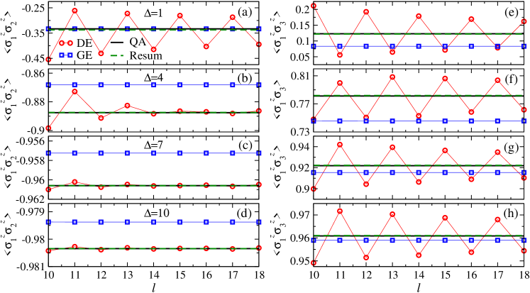
Figure 1: (Color online) Nearest [(a)–(d)] and next-nearest [(e)–(h)] neighbor $\sigma^{z}\sigma^{z}$ correlations for quenches with $\Delta=1$ [(a),(e)], $\Delta=4$ [(b),(f)],  $\Delta=7$ [(c),(g)], and $\Delta=10$ [(d),(h)]. We show results for the last nine orders of the NLCE for the diagonal ensemble (DE) and for the grand-canonical ensemble (GE). Lines joining the symbols are provided to guide the eye. For all $\Delta$’s, the GE results are essentially converged for all orders shown here. The horizontal continuous lines are the results from the quantum action method (QA) Wouters et al. ; Pozsgay et al. , and the horizontal dashed lines are the NLCE results after resummations (see text) using Wynn’s algorithm (Resum). The results of the resummations, and of the NLCE bare sums when converged, are virtually indistinguishable from those of the quantum action method. The GE results, on the other hand, are clearly different except for $\langle\sigma^{z}_{1}\sigma^{z}_{2}\rangle$ when $\Delta=1$ (see text).

As in Ref. Rigol (2014), here we perform a NLCE for observables in the DE considering clusters with up to 18 sites. For 18 sites, the sector with $S_{z}=0$ (the largest one) has 48620 states. Using parity, it is split into the even and odd sectors that have each 24310 states. Those are the largest ones in which the $XXZ$ Hamiltonian needs to be diagonalized. Since, (i) we do not need to diagonalize the initial Hamiltonian to obtain the ground state (which we know), (ii) we only need to diagonalize the sectors of the final Hamiltonian discussed previously, and (iii) the calculation of $W^{c}_{\alpha}$ is computationally trivial, our computation times are greatly reduced from those in Ref. Rigol (2014). In what follows, we denote as $\mathcal{O}^{\text{ens}}_{l}$ (the superscript “ens” stands for the ensemble used) the result obtained for an observable $\mathcal{O}$ when adding the contribution of all clusters with up to $l$ sites.

In Fig. 1, we show results for nearest [(a)–(d)] and next-nearest [(e)–(h)] neighbor $\sigma^{z}\sigma^{z}$ correlations as obtained using NLCEs for the DE. Results are reported for quenches with different values of $\Delta$ and for $l$ between 10 and 18. For $\Delta=1$, $\langle\sigma^{z}_{1}\sigma^{z}_{2}\rangle^{\text{DE}}_{l}$ [Fig. 1(a)] oscillates for even and odd values of $l$, but the amplitude of the oscillation decreases with increasing $l$. This suggests that, for larger clusters than the ones considered here, the series converges. With increasing $\Delta$, Figs. 1(b)–1(d), one can see that the amplitudes of the oscillations of $\langle\sigma^{z}_{1}\sigma^{z}_{2}\rangle^{\text{DE}}_{l}$ decrease, and (within the scale of the plots) the results appear converged. The results for $\langle\sigma^{z}_{1}\sigma^{z}_{3}\rangle^{\text{DE}}_{l}$ [Figs. 1(e)–1(h)] are qualitatively similar to those for $\langle\sigma^{z}_{1}\sigma^{z}_{2}\rangle^{\text{DE}}_{l}$, except that convergence does not appear to be achieved (oscillations are visible) for the values of $\Delta$ reported. As expected, with increasing nonlocality larger clusters are required to achieve convergence. However, as for $\langle\sigma^{z}_{1}\sigma^{z}_{2}\rangle^{\text{DE}}_{l}$, the ratio between the amplitude of the oscillations of $\langle\sigma^{z}_{1}\sigma^{z}_{3}\rangle^{\text{DE}}_{l}$ and its mean value generally decreases as $\Delta$ increases. Hence, the convergence of the NLCE calculations improves as $\Delta$ increases. This results from the fact that the ground state of the final (gapped) Hamiltonian approaches the initial (trivial) state.

The results for $\langle\sigma^{z}_{1}\sigma^{z}_{2}\rangle^{\text{DE}}_{l}$ and $\langle\sigma^{z}_{1}\sigma^{z}_{3}\rangle^{\text{DE}}_{l}$ in Fig. 1 exemplify the possible outcomes of a NLCE. In some instances, results for an observable converge to a desired accuracy within the cluster sizes accessible in the calculations [e.g., Figs. 1(b)–1(d)] and in others they do not [e.g., Figs. 1(a), 1(e)–1(h)]. In the former case, the results of the bare NLCE sums are all one needs. This was the case in Ref. Rigol (2014) for the initial temperatures selected in the quenches studied. On the other hand, if the bare NLCE sums do not converge to a desired accuracy, one can use resummation techniques to accelerate convergence and improve accuracy. Useful resummation techniques that have been implemented in the context of NLCEs can be found in Ref. Rigol et al. (2007a). Two of them, Wynn’s and Brezinski’s algorithms, provide particularly accurate results for our series. In a “cycle” of these algorithms, a series for an observable ($\mathcal{O}^{\text{DE}}_{l}$, with $l=1,\ldots,18$ in our case) is transformed into a different series with fewer elements. Each cycle is expected to improve convergence, with the last element converging to the thermodynamic limit result, but can also lead to numerical instabilities. We find that, after one cycle, the last elements provided by both algorithms are very similar to each other and representative of the outcome of the resummations (except for $\langle\sigma^{z}_{1}\sigma^{z}_{2}\rangle$ when $\Delta=1$ for which 5 cycles are required). In Fig. 1, we report Wynn’s algorithm results for the correlation functions (horizontal dashed lines).

In order to gauge the accuracy of the NLCE bare sums and resummations, we compare our results to recent analytic ones for $\langle\sigma^{z}_{1}\sigma^{z}_{2}\rangle$ Wouters et al. and $\langle\sigma^{z}_{1}\sigma^{z}_{3}\rangle$ Pozsgay et al. obtained within the quench action method Caux and Essler (2013); De Nardis et al. (2014). The latter are depicted in Fig. 1 as continuous horizontal lines. Within the scales in the plots, the NLCE results after resummations are virtually indistinguishable from the quench action results. The same is true when the NLCE bare sums appear converged, for which the results are indistinguishable from the resummed and the quench action ones.

After a quench in integrable systems, such as the $XXZ$ chain Cazalilla et al. (2011) studied here, observables are expected to relax to the predictions of a generalized Gibbs ensemble (GGE) Rigol et al. (2007c), which maximizes the entropy Jaynes (1957a, b) given the constraints imposed by the conserved quantities that make the system integrable. This has been shown to occur in numerical and analytical studies of integrable models that are mappable to noninteracting ones Rigol et al. (2007c, 2006b); Cazalilla (2006); Kollar and Eckstein (2008); Iucci and Cazalilla (2009); Fioretto and Mussardo (2010); Iucci and Cazalilla (2010); Cassidy et al. (2011); Calabrese et al. (2011); Gramsch and Rigol (2012); Cazalilla et al. (2012); Calabrese et al. (2012); Essler et al. (2012); Collura et al. (2013); Caux and Essler (2013); Fagotti (2013, 2013), where the conserved quantities have been taken to be either the occupation of the single-particle eigenstates of the noninteracting model or local quantities. In Refs. Wouters et al. ; Pozsgay et al. , it was shown that the results from the quantum action method (expected to predict the outcome of the relaxation dynamics) and from the GGE based on known local conserved quantities are different for quenches in the $XXZ$ chain. This has opened a debate as to which other conserved quantities, if any, should be included in the GGE so that it can describe observables after relaxation fagotti_essler_13 ; fagotti_collura_14 ; Mierzejewski et al. (2014); Goldstein and Andrei ; Pereira et al. ; Pozsgay .

For the quenches studied here, the differences between the quantum action method and the GGE are so small that, except for $\langle\sigma^{z}_{1}\sigma^{z}_{3}\rangle$ close to the Heisenberg point Wouters et al. , they cannot be resolved within our NLCEs. For example, (i) for $\Delta=7$ we obtain from NLCE after resummations that $\langle\sigma^{z}_{1}\sigma^{z}_{2}\rangle^{\text{NLCE}}=-0.96060$ while the quantum action predicts $\langle\sigma^{z}_{1}\sigma^{z}_{2}\rangle^{\text{QA}}=-0.960601$ and the GGE predicts $\langle\sigma^{z}_{1}\sigma^{z}_{2}\rangle^{\text{GGE}}=-0.960597$; and (ii) for $\Delta=10$ we obtain from NLCE after resummations that $\langle\sigma^{z}_{1}\sigma^{z}_{2}\rangle^{\text{NLCE}}=-0.980344$ while the quantum action predicts $\langle\sigma^{z}_{1}\sigma^{z}_{2}\rangle^{\text{QA}}=-0.9803452$ and the GGE predicts $\langle\sigma^{z}_{1}\sigma^{z}_{2}\rangle^{\text{GGE}}=-0.9803447$.

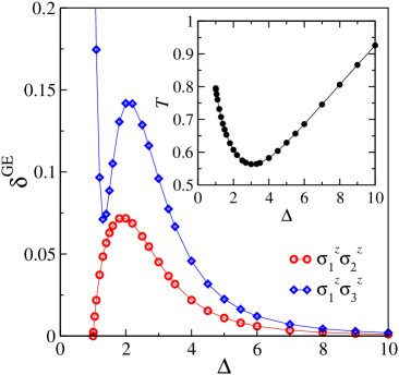
Figure 2: (Color online) Relative differences $\delta_{\sigma^{z}_{1}\sigma^{z}_{2}}$ and $\delta_{\sigma^{z}_{1}\sigma^{z}_{3}}$ between the GE and the quantum action method vs $\Delta$. The differences are seen to go to zero as $\Delta\rightarrow 1$ and $\Delta\rightarrow\infty$ and peak for $\Delta\approx 2.0$. (Inset) Effective temperature of the GE vs $\Delta$.

An important question for experiments is whether the differences between the results after equilibration following a quantum quench in an integrable system and the GE results are large enough that they can be resolved. This would allow experimentalists to prove that standard statistical mechanics ensembles are unable to describe observables in interacting integrable systems after relaxation. In order to address this question, we also compute the GE predictions for nearest- and next-nearest-neighbor $\sigma^{z}\sigma^{z}$ correlations, which we denote as $\langle\sigma^{z}_{1}\sigma^{z}_{2}\rangle^{\text{GE}}$ and $\langle\sigma^{z}_{1}\sigma^{z}_{3}\rangle^{\text{GE}}$, respectively. We impose that the GE must have the same mean energy ($E^{\text{GE}}$) and expectation value of $\hat{S}_{z}$ ($\langle\hat{S}^{z}\rangle^{\text{GE}}$), per site, as the state after the quench. Given that the $XXZ$ Hamiltonian is unchanged under a transformation $\uparrow\,\rightleftarrows\,\downarrow$, a final chemical potential $\mu=0$ ensures that $\langle\hat{S}^{z}\rangle^{\text{GE}}=0$ as in our initial state. Hence, given the energy per site after the quench ($E^{\text{DE}}$), all we need is to find the temperature $T$ at which $E^{\text{GE}}=E^{\text{DE}}$. We compute $T$ by requiring that the normalized [as in Eq. (6)] energy difference between $E^{\text{DE}}_{18}$ and $E^{\text{GE}}_{18}$ is smaller than $10^{-11}$. We should stress that, in all our calculations, $E^{\text{DE}}_{18}$ and $E^{\text{GE}}_{18}$ are fully converged within machine precision.

In the inset in Fig. 2, we plot $T$ versus $\Delta$. That plot shows that $T$ decreases as $\Delta$ departs from $1$, reaches a minimum near $\Delta\approx 3$, and then increases almost linearly with $\Delta$ for large values of $\Delta$. The latter behavior is the result of the increase of the ground-state gap with increasing $\Delta$, and the fact that the initial state is not an eigenstate of Hamiltonian Eq. (5) for any finite value of $\Delta$. This behavior is qualitatively similar to the one seen in quenches in the Bose-Hubbard model when the initial state is a Fock state with one particle per site Sorg et al. .

Results for $\langle\sigma^{z}_{1}\sigma^{z}_{2}\rangle^{\text{GE}}$ and $\langle\sigma^{z}_{1}\sigma^{z}_{3}\rangle^{\text{GE}}$ versus $l$ are plotted in Fig. 1. In all cases one can see that, for the values of $l$ reported, the NLCE results for the GE are converged within the scale of the plots. Furthermore, they are clearly different from the results after the quench in all cases but for $\langle\sigma^{z}_{1}\sigma^{z}_{2}\rangle$ and $\Delta=1$. At the Heisenberg point, the $SU(2)$ symmetry of the model results in $\langle\sigma^{z}_{1}\sigma^{z}_{2}\rangle^{\text{QA}}=\langle\sigma^{z}_{1}\sigma^{z}_{2}\rangle^{\text{GGE}}=\langle\sigma^{z}_{1}\sigma^{z}_{2}\rangle^{\text{GE}}$.

In order to quantify the differences between the results after relaxation following the quench and the GE predictions, we compute the normalized differences

$$\delta^{\text{GE}}_{\sigma^{z}_{i}\sigma^{z}_{j}}=\frac{|\langle\sigma^{z}_{i}\sigma^{z}_{j}\rangle^{\text{GE}}-\langle\sigma^{z}_{i}\sigma^{z}_{j}\rangle^{\text{QA}}|}{|\langle\sigma^{z}_{i}\sigma^{z}_{j}\rangle^{\text{QA}}|}.$$ (6)

$\delta^{\text{GE}}_{\sigma^{z}_{1}\sigma^{z}_{2}}$ is plotted in the main panel of Fig. 2 versus $\Delta$. This quantity first increases as $\Delta$ departs from 1, reaches a maximum around $\Delta=2.0$ and then decreases. This is qualitatively similar to the behavior reported in Ref. Wouters et al. for the differences between $\langle\sigma^{z}_{1}\sigma^{z}_{2}\rangle^{\text{GGE}}$ and $\langle\sigma^{z}_{1}\sigma^{z}_{2}\rangle^{\text{QA}}$. There is an important quantitative difference though, $\delta^{\text{GE}}_{\sigma^{z}_{1}\sigma^{z}_{2}}$ is much larger. $\delta^{\text{GE}}_{\sigma^{z}_{1}\sigma^{z}_{3}}$ exhibits a qualitatively similar behavior to $\delta^{\text{GE}}_{\sigma^{z}_{1}\sigma^{z}_{2}}$ except that, for $\Delta\gtrsim 1$, it first sharply decreases (from $\delta^{\text{GE}}_{\sigma^{z}_{1}\sigma^{z}_{3}}=0.32$ for $\Delta=1$) before increasing as $\delta^{\text{GE}}_{\sigma^{z}_{1}\sigma^{z}_{2}}$ does for $\Delta\gtrsim 1$. We note that, for all values of $\Delta>1$, the “memory” of the initial state (due to integrability) leads to $|\langle\sigma^{z}_{1}\sigma^{z}_{2,3}\rangle^{\text{QA}}|>|\langle\sigma^{z}_{1}\sigma^{z}_{2,3}\rangle^{\text{GE}}|$. The large values attained by $\delta^{\text{GE}}_{\sigma^{z}_{1}\sigma^{z}_{2}}$ and $\delta^{\text{GE}}_{\sigma^{z}_{1}\sigma^{z}_{3}}$ make them potentially accessible to experimental verification.

In summary, we have shown that NLCEs for the DE, recently introduced in Ref. Rigol (2014), can be used to study quenches starting from ground states or other engineered initial states of interest. Here we have studied the particular case of quenches in the (integrable) $XXZ$ chain starting from the ground state of the AF Ising chain. Our bare NLCE sums (when converged), and the results after resummations, were shown to be in excellent agreement with analytic results in the thermodynamic limit. Furthermore, we have shown that the differences between the outcome of the relaxation dynamics for $\langle\sigma^{z}_{1}\sigma^{z}_{2}\rangle$ and $\langle\sigma^{z}_{1}\sigma^{z}_{3}\rangle$ in such quenches and the thermal predictions are large enough that they could potentially be resolved in experiments.