Magnetic Reconnection in Astrophysical Environments

Abstract

Magnetic reconnection is a process that changes magnetic field topology in highly conducting fluids. Traditionally, magnetic reconnection was associated mostly with solar flares. In reality, the process must be ubiquitous as astrophysical fluids are magnetized and motions of fluid elements necessarily entail crossing of magnetic frozen in field lines and magnetic reconnection. We consider magnetic reconnection in realistic 3D geometry in the presence of turbulence. This turbulence in most astrophysical settings is of pre-existing nature, but it also can be induced by magnetic reconnection itself. In this situation turbulent magnetic field wandering opens up reconnection outflow regions, making reconnection fast. We discuss Lazarian & Vishniac (1999) model of turbulent reconnection, its numerical and observational testings, as well as its connection to the modern understanding of the Lagrangian properties of turbulent fluids. We show that the predicted dependences of the reconnection rates on the level of MHD turbulence make the generally accepted Goldreich & Sridhar (1995) model of turbulence self-consistent. Similarly, we argue that the well-known Alfvén theorem on flux freezing is not valid for the turbulent fluids and therefore magnetic fields diffuse within turbulent volumes. This is an element of magnetic field dynamics that was not accounted by earlier theories. For instance, the theory of star formation that was developing assuming that it is only the drift of neutrals that can violate the otherwise perfect flux freezing, is affected and we discuss the consequences of the turbulent diffusion of magnetic fields mediated by reconnection. Finally, we briefly address the first order Fermi acceleration induced by magnetic reconnection in turbulent fluids which is discussed in detail in the chapter by de Gouveia Dal Pino and Kowal in this volume.

1 Introduction

Magnetic fields modify fluid dynamics and it is generally believed that magnetic fields embedded in a highly conductive fluid retain their topology for all time due to the magnetic fields being frozen-in Alfven42 ; Parker79 . Nevertheless, highly conducting ionized astrophysical objects, like stars and galactic disks, show evidence of changes in topology, i.e. “magnetic reconnection”, on dynamical time scales Parker70 ; Lovelace76 ; PriestForbes02 . Historically, magnetic reconnection research was motivated by observations of the solar corona Innesetal97 ; YokoyamaShibata95 ; Masudaetal94 and this influenced attempts to find peculiar conditions conducive for flux conservation violation, e.g. special magnetic field configurations or special plasma conditions. For instance, much work has concentrated on showing how reconnection can be rapid in plasmas with very small collision rates Shayetal98 ; Drake01 ; Drakeetal06 ; Daughtonetal06 . However, it is clear that reconnection is a ubiquitous process taking place in various astrophysical environments, e.g. magnetic reconnection can be inferred from the existence of large-scale dynamo activity inside stellar interiors Parker93 ; Ossendrijver03 , as well as from the eddy-type motions in magnetohydrodynamic turbulence. Without fast magnetic reconnection magnetized fluids would behave like Jello or felt, rather than as a fluid.

In fact, solar flares Sturrock66 are just one vivid example of reconnection activity. Some other reconnection events, e.g. $\gamma$-ray bursts ZhangYan11 ; Lazarianetal04 ; Foxetal05 ; Galamaetal98 also occur in collisionless media, while others take place in collisional media. Thus attempts to explain only collisionless reconnection substantially limits astrophysical applications of the corresponding reconnection models. We also note that magnetic reconnection occurs rapidly in computer simulations due to the high values of resistivity (or numerical resistivity) that are employed at the resolutions currently achievable. Therefore, if there are situations where magnetic fields reconnect slowly, numerical simulations do not adequately reproduce astrophysical reality. This means that if collisionless reconnection is the only way to make reconnection rapid, then numerical simulations of many astrophysical processes, including those of the interstellar medium (ISM), which is collisional, are in error. Fortunately, this scary option is not realistic, as recent observations of the collisional parts of the solar atmosphere indicate fast reconnection ShibataMagara11 .

What makes reconnection enigmatic is that it is not possible to claim that reconnection must always be rapid empirically, as solar flares require periods of flux accumulation time, which correspond to slow reconnection. Thus magnetic reconnection should have some sort of trigger, which should not depend on the parameters of the local plasma. In this review we argue that the trigger is turbulence.

We may add that some recent reviews dealing with turbulent magnetic reconnection include BrowningLazarian13 and KarimabadiLazarian13 . The first one analyzes the reconnection in relation to solar flares, the other provides the comparison of the PIC simulations of the reconnection in collisionless plasmas with the reconnection in turbulent MHD regime.

In the review below we provide a simple description of the basics of magnetic reconnection and astrophysical turbulence in §2, present the theory of magnetic reconnection in the presence of turbulence and its testing in §3 and §4, respectively. Observational tests of the magnetic reconnection are described in §5 while the extensions of the reconnection theory are discussed in §6 and its astrophysical implications are summarized in §7. In §8 we present a discussion and summary of the review.

2 Basics of Magnetic Reconnection and Astrophysical Turbulence

2.1 Models of laminar reconnection

Turbulence is usually not a welcome ingredient in theoretical modeling. Turbulence carries an aura of mystery, especially magnetic turbulence, which is still a subject of ongoing debates. Thus, it is not surprising that researchers prefer to consider laminar models whenever possible.

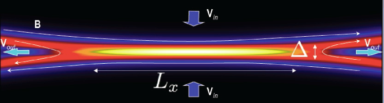
Figure 1: Sweet-Parker reconnection. Simulations of laminar reconnection from Kowaletal09 are used. The current sheet has $L_{x}$ extension, while the ejection of matter and shared component of magnetic field happens through $\Delta$. The cross-section of the reconnection is shown. Generically, the shared component of magnetic field is directed perpendicular to the picture plane. This component should be also ejected through $\Delta$.

The classical Sweet-Parker model, the first analytical model for magnetic reconnection, was proposed by Parker Parker57 and Sweet Sweet58 . Sweet-Parker reconnection has the virtue that it relies on a robust and straightforward geometry (see Figure 1). Two regions with uniform laminar magnetic fields are separated by thin current sheet. The speed of reconnection is given roughly by the resistivity divided by the sheet thickness, i.e.

$$V_{rec1}\approx\eta/\Delta.$$ (1)

One might incorrectly assume that by decreasing the current sheet thickness one can increase the reconnection rate. In fact, for steady state reconnection the plasma in the current sheet must be ejected from the edge of the current sheet at the Alfvén speed, $V_{A}$. Thus the reconnection speed is

$$V_{rec2}\approx V_{A}\Delta/L,$$ (2)

where $L$ is the length of the current sheet, which requires $\Delta$ to be large for a large reconnection speed.

In other words, we face two contradictory requirements on the outflow thickness, namely, $\Delta$ should be large so as to not constrain the outflow of plasma and $\Delta$ should be small for the Ohmic diffusivity to do its job of dissipating magnetic field lines. As a result, the steady state Sweet-Parker reconnection rate is a compromise between the two contradictory requirements. If $\Delta$ becomes small, the reconnection rate $V_{rec1}$ increases, but the insufficient outflow of plasma from the current sheet will lead to an increase in $\Delta$ and slow down the reconnection process. If $\Delta$ increases, the outflow will speed up but the oppositely directed magnetic field lines get further apart and $V_{rec1}$ drops. The slow reconnection rate limits the supply of plasma into the outflow and decreases $\Delta$. This self regulation ensures that in the steady state $V_{rec1}=V_{rec2}$ which determines both the steady state reconnection rate and the steady state $\Delta$. As a result, the overall reconnection speed is reduced from the Alfvén speed by the square root of the Lundquist number, $S\equiv L_{x}V_{A}/\eta$, i.e.

$$V_{rec,SP}=V_{A}S^{-1/2}.$$ (3)

For astrophysical conditions the Lundquist number $S$ may easily be $10^{16}$ and larger. The corresponding Sweet-Parker reconnection speed is negligible. If this sets the actual reconnection speed then we should expect magnetic field lines in the fluid not to change their topology, which in the presence of chaotic motions should result in a messy magnetic structure with the properties of Jello. On the contrary, the fast reconnection suggested by solar flares, dynamo operation etc. requires that the dependence on $S$ be erased.

A few lessons can be learned from the analysis of the Sweet-Parker reconnection. First of all, it is a self-regulated process. Second, even with the Sweet-Parker scheme the instantaneous rates of reconnection are not restricted. Indeed, under the external forcing the Ohmic annihilation rate given by $V_{rec1}$ can be arbitrary large, which, nevertheless does not mean that the time averaged rate of reconnection is also large. This should be taken into account when the probability distribution functions of currents are interpreted in terms of magnetic reconnection (see §4.5).

The low efficiency of the Sweet-Parker reconnection arises from the disparity of the scales of $\Delta$, which is determined by microphysics, i.e. depends on $\eta$, and $L_{x}$ that has a huge, i.e. astronomical, size. The introduction of plasma effects does not change this problem as in this case $\Delta$ should be of the order of the ion Larmor radius, which is $\ll L_{x}$. There are two ways to make the reconnection speed faster. One way is to reduce $L_{x}$, by changing the geometry of reconnection region, e.g. making magnetic field lines come at a sharp angle rather than in a natural Sweet-Parker way. This is called X-point reconnection. The most famous example of this is Petschek reconnection Petschek64 (see Figure 2). The other way is to extend $\Delta$ and make it comparable to $L_{x}$. Obviously, a factor different from resistivity should be involved. In this review we provide evidence that turbulence can do the job of increasing $\Delta$. However, before focusing on this process, we shall first discuss very briefly the Petschek reconnection model, which for a few decades served as the default model of fast reconnection.

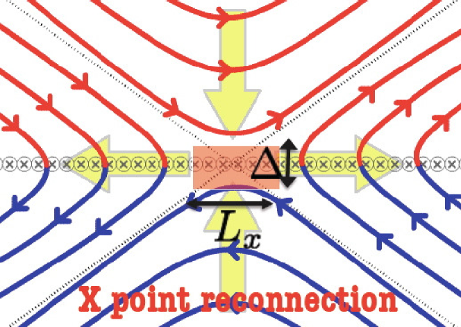
Figure 2: Petschek reconnection is an X-point reconnection where due to the formation of shocks the magnetic field lines are bent sharply towards the reconnection “point” with $L_{x}\sim\Delta$.

Figure 2 illustrates the Petschek model of reconnection. The model suggests that extended magnetic bundles come into contact over a tiny area determined by the Ohmic diffusivity. This configuration differs dramatically from the expected generic configuration when magnetic bundles try to press their way through each other. Thus the first introduction of this model raised questions of dynamical self-consistency. An X-point configuration has to persist in the face of compressive bulk forces. However, numerical simulations have shown that an initial X-point configuration of magnetic field reconnection is unstable in the MHD limit for small values of the Ohmic diffusivity Biskamp96 and the magnetic field will relax to a Sweet-Parker configuration. The physical explanation for this effect is simple. In the Petschek model shocks are required in order to maintain the geometry of the X-point. These shocks must persist and be supported by the flows driven by fast reconnection. The simulations showed that the shocks fade away and the contact region spontaneously increases.

X-point reconnection can be stabilized when the plasma is collisionless. Numerical simulations Shayetal98 ; Shayetal04 have been encouraging in this respect and created the hope that there was at last the solution of the long-standing problem of magnetic reconnection. However, there are several important issues that remain unresolved. First, it is not clear that this kind of fast reconnection persists on scales greater than the ion inertial scale Bhattacharjeeetal03 . Several numerical studies Wangetal01 ; Smithetal04 ; Fitzpatrick04 have found large scale reconnection speeds which are not fast in the sense that they show dependence on resistivity. There are countervailing analytical studies Malyshkin08 ; Shivamoggi11 which suggest that Hall X-point reconnection rates are independent of resistivity or other microscopic plasma mechanisms of line slippage, but the rates determined in these studies become small when the ion inertial scale is much less than $L_{x}$. Second, in many circumstances the magnetic field geometry does not allow the formation of X-point reconnection. For example, a saddle-shaped current sheet cannot be spontaneously replaced by an X-point. The energy required to do so is comparable to the magnetic energy liberated by reconnection, and must be available beforehand. Third, the stability of the X-point is questionable in the presence of the external random forcing, which is common, as we discuss later, for most of the astrophysical environments. Finally, the requirement that reconnection occurs in a collisionless plasma restricts this model to a small fraction of astrophysical applications. For example, while reconnection in stellar coronae might be described in this way, stellar chromospheres can not. This despite the fact that we observe fast reconnection in those environments ShibataMagara11 . More generally, Yamada Yamada07 estimated that the scale of the reconnection sheet should not exceed about 40 times the electron mean free path. This condition is not satisfied in many environments which one might naively consider to be collisionless, among them the interstellar medium. The conclusion that stellar interiors and atmospheres, accretion disks, and the interstellar medium in general does not allow fast reconnection is drastic and unpalatable.

Petschek reconnection requires an extended X-point configuration of reconnected magnetic fluxes and Ohmic dissipation concentrated within a microscopic region. As we discuss in this review (see §5), neither of these predictions were supported by solar flare observations. This suggests that neither Sweet-Parker nor Petschek models present a universally applicable mechanism of astrophysical magnetic reconnection. This does not preclude that these processes are important in particular special situations. In what follows we argue that Petschek-type reconnection may be applicable for magnetospheric current sheets or any collisionless plasma systems, while Sweet-Parker can be important for reconnection at small scales in partially ionized gas.

2.2 Turbulence in Astrophysical fluids

Neither of these models take into account turbulence, which is ubiquitous in astrophysical environments. Indeed, plasma flows at high Reynolds numbers are generically turbulent, since laminar flows are then prey to numerous linear and finite-amplitude instabilities. This is sometimes driven turbulence due to an external energy source, such as supernova in the ISM NormanFerrara96 ; Ferriere01 , merger events and AGN outflows in the intercluster medium (ICM) Subramanianetal06 ; EnsslinVogt06 ; Chandran05 , and baroclinic forcing behind shock waves in interstellar clouds. In other cases, the turbulence is spontaneous, with available energy released by a rich array of instabilities, such as the MRI in accretion disks BalbusHawley98 , the kink instability of twisted flux tubes in the solar corona GalsgaardNordlund97a ; GerrardHood03 , etc. Whatever its origin, observational signatures of astrophysical turbulence are seen throughout the universe. The turbulent cascade of energy leads to long “inertial ranges” with power-law spectra that are widely observed, e.g. in the solar wind Leamonetal98 ; Baleetal05 , and in the ICM Schueckeretal04 ; VogtEnsslin05 .

Figure 3 illustrates the so-called “Big Power Law in the Sky” of the electron density fluctuations. The original version of the law was presented by Armstrong et al. Armstrongetal95 for electron scattering and scintillation data. It was later extended by Chepurnov et al. ChepurnovLazarian10 who used Wisconsin H$\alpha$ Mapper (WHAM) electron density data. We clearly see the power law extending over many orders of of spatial scales and suggesting the existence of turbulence in the interstellar medium. With more surveys, with more developed techniques we are getting more evidence of the turbulent nature of astrophysical fluids. For instance, for many years non-thermal line Doppler broadening of the spectral lines was used as an evidence of turbulence. The development of new techniques, namely, Velocity Channel Analysis (VCA) and Velocity Correlation Spectrum (VCS) in a series of papers by Lazarian & Pogosyan LazarianPogosyan00 ; LazarianPogosyan04 ; LazarianPogosyan06 ; LazarianPogosyan08 enabled researchers to use HI and CO spectral lines to obtain the power spectra of turbulent velocities (see Lazarian09 for a review and references therein).

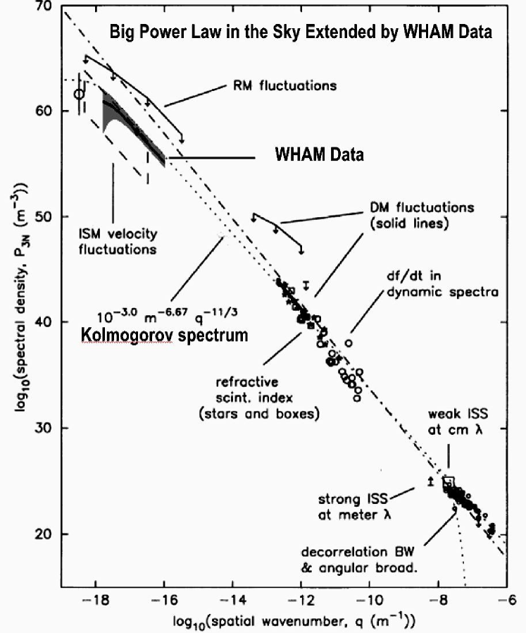
Figure 3: Turbulence in the interstellar gas of the Milky Way as revealed by electron density fluctuations. “Big Power Law in the Sky” Armstrongetal95 extended using WHAM data. The slope corresponds to that of Kolmogorov turbulence. From ChepurnovLazarian10 .

As turbulence is known to change dramatically many processes, in particular, diffusion and transport processes, it is natural to pose the question to what extent the theory of astrophysical reconnection must take into account the pre-existing turbulent environment. We note that even if the plasma flow is initially laminar, kinetic energy release by reconnection due to some slower plasma process is expected to generate vigorous turbulent motion in high Reynolds number fluids.

2.3 MHD description of plasma motions

Turbulence in plasma happens at many scales, from the largest to those below the proton Larmor radius. The effect of turbulence on magnetic reconnection is different for different types of turbulence. For instance, micro turbulence can change the microscopic resistivity of plasmas and induce anomalous resistivity effects (see Vekshteinetal70 ). In this review we advocate the idea that for solving the problem of magnetic reconnection in most astrophysical important cases the approach invoking MHD rather than plasma turbulence is adequate. To provide an initial support for this point, we shall reiterate a few known facts about the applicability of MHD approximation (Kulsrud83 , Eyinketal11 ). Below we argue that MHD description is applicable to many settings that include both collisional and collisionless plasmas, provided that we deal with plasmas at sufficiently large scales. To describe magnetized plasma dynamics one should deal with three characteristic length-scales: the ion gyroradius $\rho_{i},$ the ion mean-free-path length $\ell_{mfp,i}$ arising from Coulomb collisions, and the scale $L$ of large-scale variation of magnetic and velocity fields.

One case of reconnection that is clearly not dealt with by the popular models of collisionless reconnection (see above) is the “strongly collisional” plasma with $\ell_{mfp,i}\ll\rho_{i}$. This is the case e.g. of star interiors and most accretion disk systems. For such “strongly collisional” plasmas a standard Chapman-Enskog expansion provides a fluid description of the plasma Braginsky65 , with a two-fluid model for scales between $\ell_{mfp,i}$ and the ion skin-depth $\delta_{i}=\rho_{i}/\sqrt{\beta_{i}}$ and an MHD description at scales much larger than $\delta_{i}$. This is the most obvious case of MHD description for plasmas.

Hot and rarefied astrophysical plasmas are often “weakly collisional” with $\ell_{mfp,i}\gg\rho_{i}$. Indeed, the relation that follows from the standard formula for the Coulomb collision frequency (e.g. see Fitzpatrick11 , Eq. 1.25) is

$$\frac{\ell_{mfp,i}}{\rho_{i}}\propto\frac{\Lambda}{\ln\Lambda}\frac{V_{A}}{c},$$ (4)

where $\Lambda=4\pi n\lambda_{D}^{3}$ is the plasma parameter, or the number of particles within the Debye screening sphere, which indicates that $\Lambda$ can be very large. Typical values for some weakly coupled cases are shown in Table LABEL:tab:parameters Eyinketal11 .

Table 1: Representative Parameters for Some Weakly-Coupled Astrophysical Plasmas (from Eyinketal11 )

Parameter	warm ionized	post-CME	solar wind at
	ISM${\,\!}^{a}$	current sheets${\,\!}^{b}$	magnetosphere${\,\!}^{c}$
density $n,\,cm^{-3}$	.5	$7\times 10^{7}$	10
temperature $T,\,eV$	.7	$10^{3}$	10
plasma parameter $\Lambda$	$4\times 10^{9}$	$2\times 10^{10}$	$5\times 10^{10}$
ion thermal velocity $v_{th,i},\,cm/s$	$10^{6}$	$3\times 10^{7}$	$5\times 10^{6}$
ion mean-free-path $\ell_{mfp,i},\,cm$	$6\times 10^{11}$	$10^{10}$	$7\times 10^{12}$
magnetic diffusivity $\lambda,\,cm^{2}/s$	$10^{7}$	$8\times 10^{2}$	$6\times 10^{5}$
magnetic field $B,\,G$	$10^{-6}$	1	$10^{-4}$
plasma beta $\beta$	14	3	1
Alfvén speed $V_{A},\,cm/s$	$3\times 10^{5}$	$3\times 10^{7}$	$7\times 10^{6}$
ion gyroradius $\rho_{i},\,cm$	$10^{8}$	$3\times 10^{3}$	$6\times 10^{6}$
large-scale velocity $U,\,cm/s$	$10^{6}$	$4\times 10^{6}$	$5\times 10^{6}$
large length scale $L,\,cm$	$10^{20}$	$5\times 10^{10}$	$10^{8}$
Lundquist number $S_{L}=\frac{V_{A}L}{\lambda}$	$3\times 10^{18}$	$2\times 10^{15}$	$10^{9}$
resistive length${\,\!}^{*}$ $\ell_{\eta}^{\perp},\,cm$	$5\times 10^{5}$	1	20
${\,\!}^{a}$NormanFerrara96 ; Ferriere01      ${\,\!}^{b}$Bemporad08      ${\,\!}^{c}$Zimbardoetal10
*This nominal resistive scale is calculated from $\ell_{\eta}^{\perp}\simeq L(V_{A}/U)S_{L}^{-3/4}$, assuming GS95 turbulence holds
down to that scale, and should not be taken literally when $\ell_{\eta}^{\perp}<\rho_{i}.$

For the “weakly collisional” but well magnetized plasmas one can invoke the expansion over the small ion gyroradius. This results in the “kinetic MHD equations” for lengths much larger than $\rho_{i}$. The difference between these equations and the MHD ones is that the pressure tensor in the momentum equation is anisotropic, with the two components $p_{\|}$ and $p_{\perp}$ of the pressure parallel and perpendicular to the local magnetic field direction Kulsrud83 . “Weakly collisional”, i.e. $L\gg\ell_{mfp,i}.$, and collisionless, i.e. $\ell_{mfp,i}\gg L$ systems have been studied recently Kowaletal11 ; SantosLimaetal13 . While the direct collisions are infrequent, compressions of the magnetic field induces anisotropies, as a consequence of the adiabatic invariant conservation, in the phase space particle distribution. This induces instabilities that act upon plasma causing particle scattering SchekochihinCowley06 ; LazarianBeresnyak06 . Thus instead of Coulomb collisional frequency a new frequency of scattering is invoked. In other words, particles do not interact between each other, but each particle interacts with the ensemble of small scale perturbations induced by instabilities in the compressed magnetized plasmas. By adopting the in-situ measured distribution of particles in the collisionless solar wind Santos-Lima et al. SantosLimaetal13 showed numerically that the dynamics of such plasmas is identical to that of MHD.

Even without invoking instabilities, one can approach “weakly collisional” plasmas solving for the magnetic field using an ideal induction equation, if one ignores all collisional effects. In many cases, e.g. in the ISM and the magnetosphere (see Table LABEL:tab:parameters) the resistive length-scale $\ell_{\eta}^{\perp}$ is much smaller than both $\rho_{i}$ and $\rho_{e}\approx\frac{1}{43}\rho_{i}$. Magnetic field-lines are, at least formally, well “frozen-in” on these scales. In the “weakly collisional” case the“kinetic MHD” description can be simplified at scales greater than $\ell_{mfp,i}$ by including the Coulomb collision operator and making a Chapman-Enskog expansion. This reproduces a fully MHD description at those large scales. The idealized warm ionized phase of ISM represents “weakly collisional” plasmas in Table LABEL:tab:parameters.

We can also note that additional simplifications that justify the MHD approach occur if the turbulent fluctuations are small compared to the mean magnetic field, and having length-scales parallel to the mean field much larger than perpendicular length-scales. Treating wave frequencies that are low compared to the ion cyclotron frequency we enter the domain of “gyrokinetic approximation” which is commonly used in fusion plasmas. This approximation was advocated for application in astrophysics by Schekochihinetal07 ; Schekochihinetal09 .

For the “gyrokinetic approximation” at length-scales larger than the ion gyroradius $\rho_{i}$ the incompressible shear-Alfvén wave modes get decoupled from the compressive modes and can be described by the simple “reduced MHD” (RMHD) equations. As we argue later in the review, the shear-Alfvén modes are the modes that induce fast magnetic reconnection, while the other modes are of auxiliary importance for the process.

All in all, our considerations in this part of the review support the generally accepted notion that the MHD approximation is adequate for most astrophysical fluids at sufficiently large scales. A lot of work on reconnection is concentrated on the small scale dynamics, but if magnetic reconnection is determined by large scale motions, as we argue in this review, then the MHD description of magnetic reconnection is appropriate.

2.4 Modern understanding of MHD turbulence

Within this volume MHD turbulence is described in the chapter by Beresnyak & Lazarian (see also a description of MHD turbulence in the star formation context in the chapter by H. Vazquez-Semadeni). Therefore in presenting the major MHD turbulence results that are essential for our further derivation in the review, we shall be very brief. We will concentrate on Alfvénic modes, while disregarding the slow and fast magnetosonic modes that in principle contribute to MHD turbulence ChoLazarian02 ; ChoLazarian03 ; KowalLazarian10 . The interaction between the modes is in many cases not significant, which allows the separate treatment of Alfvén modes ChoLazarian02 ; GoldreichSridhar95 ; LithwickGoldreich01 .

While having a long history of competing ideas, the theory of MHD turbulence has become testable recently due to the advent of numerical simulations (see Biskamp03 ) which confirmed the prediction of magnetized Alfvénic eddies being elongated in the direction of the local magnetic field (see Shebalinetal83 ; Higdon84 ) and provided results consistent with the quantitative relations for the degree of eddy elongation obtained in the fundamental study by GoldreichSridhar95 (henceforth GS95).

The relation between the parallel and perpendicular dimensions of eddies in GS95 picture are presented by the so called critical balance condition, namely,

$$\ell_{\|}^{-1}V_{A}\sim\ell_{\bot}^{-1}\delta u_{\ell},$$ (5)

where $\delta u_{\ell}$ is the eddy velocity, while $\ell_{\|}$ and $\ell_{\bot}$ are, respectively, eddy scales parallel and perpendicular to the local direction of magnetic field. The local system of reference is that determined by the direction of magnetic field at the scale in the vicinity of the eddy. It should be definitely distinguished from the mean magnetic field reference frame LithwickGoldreich01 ; LazarianVishniac99 ; ChoVishniac00 ; MaronGoldreich01 ; Choetal02 , where no universal relations between the eddy scale exist. This is very natural, as small scale turnover eddies can be influenced only by the magnetic field around these eddies.

The motions perpendicular to the local magnetic field are essentially hydrodynamic. Therefore, combining (5) with the Kolmogorov cascade notion, i.e. that the energy transfer rate is $\delta u^{2}_{\ell}/(\ell_{\bot}/\delta u_{\ell})=const$ one gets $\delta u_{\ell}\sim\ell_{\bot}^{1/3}$, which coincides with the known Kolmogorov relation between the turbulent velocity and the scale. For the relation between the parallel and perpendicular scales one gets

$$\ell_{\|}\propto L_{i}^{1/3}\ell_{\bot}^{2/3},$$ (6)

where $L_{i}$ is the turbulence injection scale. Note that recent measurements of anisotropy in the solar wind are consistent with Eq. (6) Podesta10 ; Wicksetal10 ; Wicksetal11 .

In its original form the GS95 model was proposed for energy injected isotropically with velocity amplitude $u_{L}=V_{A}$. If the turbulence is injected at velocities $u_{L}\ll V_{A}$ (or anisotropically with $L_{i,\|}\ll L_{i,\bot}$), then the turbulent cascade is weak and $\ell_{\bot}$ decreases while $\ell_{\|}=L_{i}$ stays the same LazarianVishniac99 ; MontgomeryMatthaeus95 ; Galtieretal00 ; NgBhattacharjee96 . In other words, as a result of the weak cascade the eddies become thinner, but preserve the same length along the local magnetic field. It is possible to show that the interactions within weak turbulence increase and transit to the regime of the strong MHD turbulence at the scale

$$l_{trans}\sim L_{i}(u_{L}/V_{A})^{2}\equiv L_{i}M_{A}^{2}~{}~{}~{}M_{A}<1$$ (7)

and the velocity at this scale is $v_{trans}=u_{L}M_{A}$, with $M_{A}=u_{L}/V_{A}\ll 1$ beeing the Alfvénic Mach number of the turbulence LazarianVishniac99 ; Lazarian06 . Thus, weak turbulence has a limited, i.e. $[L_{i},L_{i}M_{A}^{2}]$ inertial range and at small scales it transits into the regime of strong turbulence.

Table 2 illustrates different regimes of MHD turbulence both when it is injected isotropically at superAlfvénic and subAlfvénic velocities. Naturally, superAlfvénic turbulence at large scales is similar to the ordinary hydrodynamic turbulence, as weak magnetic fields cannot strongly affect turbulent motions. However, at the scale

$$l_{A}=L_{i}(V_{A}/u_{L})^{3}=L_{i}M_{A}^{-3}~{}~{}~{}M_{A}>1$$ (8)

the motions become Alfvénic.

Table 2: Regimes and ranges of MHD turbulence.

Type	Injection	Range	Motion	Ways
of MHD turbulence	velocity	of scales	type	of study
Weak	$u_{L}<V_{A}$	$[L_{i},L_{i}M_{A}^{2}]$	wave-like	analytical
Strong
subAlfvénic	$u_{L}<V_{A}$	$[L_{i}M_{A}^{2},l_{min}]$	eddy-like	numerical
Strong
superAlfvénic	$u_{L}>V_{A}$	$[l_{A},l_{min}]$	eddy-like	numerical
$L_{i}$ and $l_{min}$ are injection and dissipation scales, respectively
$M_{A}\equiv u_{L}/V_{A}$.

In this review we address the reconnection mediated by turbulence. For this the regime of weak, i.e. wave-like, perturbations can be an important part of the dynamics. A description of MHD turbulence that incorporates both weak and strong regimes was presented in LazarianVishniac99 (henceforth LV99). In the range of length-scales where turbulence is strong, this theory implies that

$$\ell_{\|}\approx L_{i}\left(\frac{\ell_{\bot}}{L_{i}}\right)^{2/3}M_{A}^{-4/3}$$ (9)

$$\delta u_{\ell}\approx u_{L}\left(\frac{\ell_{\bot}}{L_{i}}\right)^{1/3}M_{A}^{1/3},$$ (10)

when the turbulence is driven isotropically on a scale $L_{i}$ with an amplitude $u_{L}$. These are equations that we will use further to derive the magnetic reconnection rate.

Here we do not discuss attempts to modify GS95 theory by adding concepts like “dynamical alignment”, “polarization”, “non-locality” Boldyrev06 ; BeresnyakLazarian06 ; BeresnyakLazarian09 ; Gogoberidze07 . First of all, those do not change the nature of turbulence to affect the reconnection of the weakly turbulent magnetic field. Indeed, in LV99 the calculations were provided for a wide range of possible models of anisotropic Alfvénic turbulence and provided fast reconnection. Moreover, more recent studies BeresnyakLazarian10 ; Beresnyak11 ; Beresnyak12 support the GS95 model. A more detailed discussion of MHD turbulence can be found in the recent review (e.g. BrandenburgLazarian13 ) and in Beresnyak and Lazarian’s Chapter in this volume.

GS95 presents a model of 3D MHD turbulence that exists in our 3D world. Historically, due to computational reasons, many MHD related studies were done in 2D. The problem of such studies in application to magnetic turbulence is that shear Alfvén waves that play the dominant role for 3D MHD turbulence are entirely lacking in 2D. Furthermore, all magnetized turbulence in 2D is transient, because the dynamo mechanism required to sustain magnetic fields is lacking in 2D Zeldovich57 . Thus the relation of 2D numerical studies invoking MHD turbulence, e.g. magnetic reconnection in 2D turbulence, and the processes in the actual 3D geometry is not clear. A more detailed discussion of this point can be found in Eyinketal11 .

3 Magnetic reconnection in the presence of turbulence

3.1 Initial attempts to invoke turbulence to accelerate magnetic reconnection

The first attempts to appeal to turbulence in order to enhance the reconnection rate were made more than 40 years ago. For instance, some papers have concentrated on the effects that turbulence induces on the microphysical level. In particular, Speiser Speiser70 showed that in collisionless plasmas the electron collision time should be replaced with the electron retention time in the current sheet. Also Jacobson Jacobson84 proposed that the current diffusivity should be modified to include the diffusion of electrons across the mean field due to small scale stochasticity. However, these effects are insufficient to produce reconnection speeds comparable to the Alfvén speed in most astrophysical environments.

“Hyper-resistivity” Strauss86 ; BhattacharjeeHameiri86 ; HameiriBhattacharjee87 ; DiamondMalkov03 is a more subtle attempt to derive fast reconnection from turbulence within the context of mean-field resistive MHD. The form of the parallel electric field can be derived from magnetic helicity conservation. Integrating by parts one obtains a term which looks like an effective resistivity proportional to the magnetic helicity current. There are several assumptions implicit in this derivation. The most important objection to this approach is that by adopting a mean-field approximation, one is already assuming some sort of small-scale smearing effect, equivalent to fast reconnection. Furthermore, the integration by parts involves assuming a large scale magnetic helicity flux through the boundaries of the exact form required to drive fast reconnection. The problems of the hyper-resistivity approach are discussed in detail in Eyinketal11 .

A more productive development was related to studies of instabilities of the reconnection layer. Strauss Strauss88 examined the enhancement of reconnection through the effect of tearing mode instabilities within current sheets. However, the resulting reconnection speed enhancement is roughly what one would expect based simply on the broadening of the current sheets due to internal mixing. Waelbroeck Waelbroeck89 considered not the tearing mode, but the resistive kink mode to accelerate reconnection. The numerical studies of tearing have become an important avenue for more recent reconnection research Loureiroetal09 ; Bhattacharjeeetal09 . As we discuss later in realistic 3D settings tearing instability develops turbulence Karimabadietal13 ; Beresnyak13b ) which induces a transfer from laminar to turbulent reconnection.

Finally, a study of 2D magnetic reconnection in the presence of external turbulence was done by MatthaeusLamkin85 ; MatthaeusLamkin86 . An enhancement of the reconnection rate was reported, but the numerical setup precluded the calculation of a long term average reconnection rate. As we discussed in §2.1 bringing in the Sweet-Parker model of reconnection magnetic field lines closer to each other one can enhance the instantaneous reconnection rate, but this does not mean that averaged long term reconnection rate increases. This, combined with the absence of the theoretical predictions of the expected reconnection rates makes it difficult to make definitive conclusions from the study. Note that, as we discussed in §2.4, the nature of turbulence is different in 2D and 3D. Therefore, the effects accelerating magnetic reconnection mentioned in the study, i.e. formation of X-points, compressions, may be relevant for 2D set ups, but not relevant for the 3D astrophysical reconnection. These effects are not invoked in the model of the turbulent reconnection that we discuss below. We also may note that a more recent study along the approach in MatthaeusLamkin85 is one in Watsonetal07 , where the effects of small scale turbulence on 2D reconnection were studied and no significant effects of turbulence on reconnection were reported for the setup chosen by the authors.

In a sense, the above study is the closest predecessor of LV99 work that we deal below. However, there are very substantial differences between the approach of LV99 and MatthaeusLamkin85 . For instance, LV99, as is clear from the text below, uses an analytical approach and, unlike MatthaeusLamkin85 , (a) provides analytical expressions for the reconnection rates; (b) identifies the broadening arising from magnetic field wandering as the mechanism for inducing fast reconnection; (c) deals with 3D turbulence and identifies incompressible Alfvénic motions as the driver of fast reconnection.

3.2 Model of magnetic reconnection in weakly turbulent media

As we discussed earlier, considering astrophysical reconnection in laminar environments is not normally realistic. As a natural generalization of the Sweet-Parker model it is appropriate to consider 3D magnetic field wandering induced by turbulence as in LV99. The corresponding model of magnetic reconnection is illustrated by Figure 4.

Figure 4: Upper plot: Sweet-Parker model of reconnection. The outflow is limited to a thin width $\delta$, which is determined by Ohmic diffusivity. The other scale is an astrophysical scale $L\gg\delta$. Magnetic field lines are assumed to be laminar. Middle plot: Turbulent reconnection model that accounts for the stochasticity of magnetic field lines. The stochasticity introduced by turbulence is weak and the direction of the mean field is clearly defined. The outflow is limited by the diffusion of magnetic field lines, which depends on macroscopic field line wandering rather than on microscales determined by resistivity. Low plot: An individual small scale reconnection region. The reconnection over small patches of magnetic field determines the local reconnection rate. The global reconnection rate is substantially larger as many independent patches reconnect simultaneously. Conservatively, the LV99 model assumes that the small scale events happen at a slow Sweet-Parker rate. Following Lazarianetal04 .

Like the Sweet-Parker model, the LV99 model deals with a generic configuration, which should arise naturally as magnetic flux tubes try to make their way one through another. This avoids the problems related to the preservation of wide outflow which plagues attempts to explain magnetic reconnection via Petscheck-type solutions. In this model if the outflow of reconnected flux and entrained matter is temporarily slowed down, reconnection will also slow down, but, unlike Petscheck solution, will not change the nature of the solution.

The major difference between the Sweet-Parker model and the LV99 model is that while in the former the outflow is limited by microphysical Ohmic diffusivity, in the latter model the large-scale magnetic field wandering determines the thickness of outflow. Thus LV99 model does not depend on resistivity and, depending on the level of turbulence, can provide both fast and slow reconnection rates. This is a very important property for explaining observational data related to reconnection flares.

For extremely weak turbulence, when the range of magnetic field wandering becomes smaller than the width of the Sweet-Parker layer $LS^{-1/2}$, the reconnection rate reduces to the Sweet-Parker rate, which is the ultimate slowest rate of reconnection. As a matter of fact, this slow rate holds only for Lundquist numbers less than $S_{c}$, the critical value for tearing mode instability of the Sweet-Parker solution. At higher Lundquist numbers, self-generated turbulence will be the inevitable outcome of unstable breakdown of the Sweet-Parker current sheet and this will yield the minimal reconnection rate in an otherwise quiet environment (see, in particular, Beresnyak13b ).

We note that LV99 does not appeal to a chaotic field created within a hydrodynamic weakly magnetized turbulent flow. On the contrary, the model considers the case of a large scale, well-ordered magnetic field, of the kind that is normally used as a starting point for discussions of reconnection. In the presence of turbulence one expects that the field will have some small scale ‘wandering’ and this effect changes the nature of magnetic reconnection.

Ultimately, the magnetic field lines will dissipate due to microphysical effects, e.g. Ohmic resistivity. However, it is important to understand that in the LV99 model only a small fraction of any magnetic field line is subject to direct Ohmic annihilation. The fraction of magnetic energy that goes directly into heating the fluid approaches zero as the fluid resistivity vanishes. In addition, 3D Alfvénic turbulence enables many magnetic field lines to enter the reconnection zone simultaneously, which is another difference between 2D and 3D reconnection.

3.3 Opening up of the outflow region via magnetic field wandering

To get the reconnection speed one should calculate the thickness of the outflow $\Delta$ that is determined by the magnetic field wandering. This was done in LV99, where the scaling relations for the wandering field lines were established.

The scaling relations for Alfvénic turbulence discussed in §2.4 allow us to calculate the rate of magnetic field spreading. A bundle of field lines confined within a region of width $y$ at some particular point spreads out perpendicular to the mean magnetic field direction as one moves in either direction following the local magnetic field lines. The rate of field line diffusion is given by

$${d\langle y^{2}\rangle\over dx}\sim{\langle y^{2}\rangle\over\lambda_{\|}},$$ (11)

where $\lambda_{\|}^{-1}\approx\ell_{\|}^{-1}$, $\ell_{\|}$ is the parallel scale and the corresponding transversal scale, $\ell_{\perp}$, is $\sim\langle y^{2}\rangle^{1/2}$, and $x$ is the distance along an axis parallel to the magnetic field. Therefore, using equation (9) one gets

$${d\langle y^{2}\rangle\over dx}\sim L_{i}\left({\langle y^{2}\rangle\over L_{i}^{2}}\right)^{2/3}\left({u_{L}\over V_{A}}\right)^{4/3}$$ (12)

where we have substituted $\langle y^{2}\rangle^{1/2}$ for $\ell_{\perp}$. This expression for the diffusion coefficient will only apply when $y$ is small enough for us to use the strong turbulence scaling relations, or in other words when $\langle y^{2}\rangle<L_{i}^{2}(u_{L}/V_{A})^{4}$. Larger bundles will diffuse at the rate of $L_{i}^{2}(u_{L}/V_{A})^{4}$, which is the maximal rate. For $\langle y^{2}\rangle$ small, equation (12) implies that a given field line will wander perpendicular to the mean field line direction by an average amount

$$\langle y^{2}\rangle^{1/2}\approx{x^{3/2}\over L_{i}^{1/2}}\left({u_{L}\over V_{A}}\right)^{2}~{}~{}~{}x<L_{i}$$ (13)

in a distance $x$. The fact that the rms perpendicular displacement grows faster than $x$ is significant. It implies that if we consider a reconnection zone, a given magnetic flux element that wanders out of the zone has only a small probability of wandering back into it. We also note that $y$ proportional to $x^{3/2}$ is a consequence of the process of Richardson diffusion that we discuss below.

When the turbulence injection scale is less than the extent of the reconnection layer, i.e. $Lx\gg L_{i}$ magnetic field wandering obeys the usual random walk scaling with $L_{x}/L_{i}$ steps and the mean squared displacement per step equal to $L_{i}^{2}(u_{L}/V_{A})^{4}$. Therefore

$$\langle y^{2}\rangle^{1/2}\approx(L_{i}x)^{1/2}(u_{L}/V_{A})^{2}~{}~{}~{}x>L_{i}$$ (14)

Using Eqs. (13) and (14) one can derive the thickness of the outflow $\Delta$ (see Figure 1) and obtain (LV99):

$$V_{rec}\approx V_{A}\min\left[\left({L_{x}\over L_{i}}\right)^{1/2},\left({L_{i}\over L_{x}}\right)^{1/2}\right]M_{A}^{2},$$ (15)

where $V_{A}M_{A}^{2}$ is proportional to the turbulent eddy speed. This limit on the reconnection speed is fast, both in the sense that it does not depend on the resistivity, and in the sense that it represents a large fraction of the Alfvén speed when $L_{i}$ and $L_{x}$ are not too different and $M_{A}$ is not too small. At the same time, Eq. (15) can lead to rather slow reconnection velocities for extreme geometries or small turbulent velocities. This, in fact, is an advantage, as this provides a natural explanation for flares of reconnection, i.e. processes which combine both periods of slow and fast magnetic reconnection. The parameters in Eq. (15) can change in the process of magnetic reconnection, as the energy injected by the reconnection will produce changes in $M_{A}$ and $L_{i}$. In fact, we claim that in the process of magnetic reconnection and the energy injection that this entails for magnetically dominated plasmas, one can expect both $L_{i}\rightarrow L_{x}$ and $M_{A}\rightarrow 1$, which will induce efficient reconnection with $V_{rec}\sim V_{A}$.

3.4 Richardson diffusion and LV99 model

It is well known that at scales larger than the turbulence injection scale the fluid exhibits diffusive properties. At the same time, at scales less than the turbulence injection scale the properties of diffusion are different. Since the velocity difference increases with separation, one expects that accelerated diffusion, or super diffusion should take place. This process was first described by Richardson for hydrodynamic turbulence. A similar effect is present for MHD turbulence (see EyinkBenveniste13 and references therein).

Richardson diffusion can be illustrated with a simple model. Consider the growth of the separation between two particles $dl(t)/dt\sim v(l),$ which for Kolmogorov turbulence is $\sim\alpha_{t}l^{1/3}$, where $\alpha_{t}$ is proportional to the energy cascading rate, i.e. $\alpha_{t}\approx V_{L}^{3}/L$ for turbulence injected with superAlvénic velocity $V_{L}$ at the scale $L$. The solution of this equation is

$$l(t)=[l_{0}^{2/3}+\alpha_{t}(t-t_{0})]^{3/2},$$ (16)

which at late times leads to Richardson diffusion or $l^{2}\sim t^{3}$ compared with $l^{2}\sim t$ for ordinary diffusion.

Richardson diffusion provides explosive separation of magnetic field lines. It is clear from Eq. (16) that the separation of magnetic field lines does not depend on the initial separation $l_{0}$ after sufficiently long intervals of time $t$. Potentially, one can make $l_{0}$ very small, but, realistically, $l_{0}$ should not be smaller than the scale of the marginally damped eddies $l_{damp}$, as the derivation of the Richardson diffusion assumes the existence of inertial-range turbulence at the scales under study. At scales less than $l_{damp}$ diffusion is determined by the shearing by the marginally damped eddies. This is known to result in Lagrangian chaos and Lyapunov exponential separation of the points. Separation at long times in this regime does depend on the initial separation of points. In other words, in realistic turbulence up to the scale of $l_{damp}$ the distance between the points preserves the memory of the initial separation of points, while at scales larger than $l_{damp}$ this dependence is washed out.

Richardson diffusion is important in terms of spreading magnetic fields. In fact, the magnetic field line spread as a function of the distance measured along magnetic field lines, which we discussed in the previous subsection, is also a manifestation of Richardson diffusion, but in space rather than in time. Below, we, however, use the time dependence of Richardson diffusion to re-derive the LV99 results.

Sweet-Parker reconnection can serve again as our guide. There we deal with Ohmic diffusion. The latter induces the mean-square distance across the reconnection layer that a magnetic field-line can diffuse by resistivity in a time $t$ given by

$$\langle y^{2}(t)\rangle\sim\lambda t.$$ (17)

where $\lambda=c^{2}/4\pi\sigma$ is the magnetic diffusivity. The field lines are advected out of the sides of the reconnection layer of length $L_{x}$ at a velocity of order $V_{A}$. Therefore, the time that the lines can spend in the resistive layer is the Alfvén crossing time $t_{A}=L_{x}/V_{A}$. Thus, field lines that can reconnect are separated by a distance

$$\Delta=\sqrt{\langle y^{2}(t_{A})\rangle}\sim\sqrt{\lambda t_{A}}=L_{x}/\sqrt{S},$$ (18)

where $S$ is Lundquist number. Combining Eqs. (2) and (18) one gets again the well-known Sweet-Parker result, $v_{rec}=V_{A}/\sqrt{S}$.

Below, following Eyinketal11 (henceforth ELV11) we provide a different derivation of the reconnection rate within the LV99 model. We make use of the fact that in Richardson diffusion Kupiainen03 the mean squared separation of particles $\langle|x_{1}(t)-x_{2}(t)|^{2}\rangle\approx\epsilon t^{3}$, where $t$ is time, $\epsilon$ is the energy cascading rate and $\langle...\rangle$ denote an ensemble averaging. For subAlfvénic turbulence $\epsilon\approx u_{L}^{4}/(V_{A}L_{i})$ (see LV99) and therefore analogously to Eq. (18) one can write

$$\Delta\approx\sqrt{\epsilon t_{A}^{3}}\approx L(L/L_{i})^{1/2}M_{A}^{2}$$ (19)

where it is assumed that $L<L_{i}$. Combining Eqs. (2) and (19) one gets

$$v_{rec,LV99}\approx V_{A}(L/L_{i})^{1/2}M_{A}^{2}.$$ (20)

in the limit of $L<L_{i}$. Similar considerations allow to recover the LV99 expression for $L>L_{i}$, which differs from Eq. (20) by the change of the power $1/2$ to $-1/2$. These results coincide with those given by Eq. (15).

3.5 Role of plasma effects for magnetic reconnection

In the LV99 model the outflow is determined by turbulent motions that are determined by the motions on the small scales. The small scale physics in this situation gets irrelevant if the level of turbulence is fixed. Following Eyinketal11 it is possible to define the criterion for the Hall effect to be important within the LV99 reconnection model.

Using the GS95 model one can estimate the pointwise ratio of the Hall electric field to the MHD motional field as

$$\frac{J/en}{u_{L}}\simeq\frac{c\delta B(\ell_{\eta}^{\perp})/4\pi ne\ell_{\eta}^{\perp}}{u_{L}}\simeq\frac{\delta_{i}}{L_{i}}M_{A}S_{L}^{1/2}$$ (21)

where $S_{L}=V_{A}L_{i}/\lambda$ is the Lundquist number based on the forcing length-scale of the turbulence and $M_{A}=u_{L}/V_{A}$ is the Alfvénic Mach number, $\ell_{\eta}^{\perp}$ is the resistive cutoff length, $J$ current density, and $n$ electron density. This can be expressed as a ratio $(J/en)/u_{L}\simeq\delta_{i}/\delta_{T}$ of ion skin depth to the turbulent Taylor scale

$$\delta_{T}=L_{i}M_{A}^{-1}S_{L}^{-1/2},$$ (22)

which can be interpreted heuristically as the current sheet thickness of small-scale Sweet-Parker reconnection layers. If the magnetic diffusivity in the definition of the Lundquist number is assumed to be that based on the Spitzer resistivity, given by $\lambda=\delta_{e}^{2}v_{th,e}/\ell_{ei}$ where $\delta_{e}$ is the electron skin depth, $v_{th,e}$ is the electron thermal velocity, and $\ell_{ei}$ is the electron mean-free-path length for collisions with ions, then $S_{L}=\left(\frac{m_{e}}{m_{i}}\right)^{1/2}\beta^{-1/2}\left(\frac{\ell_{ei}}{\delta_{e}}\right)^{2}\left(\frac{L_{i}}{\ell_{ei}}\right),$ with $\beta=v_{th,i}^{2}/V_{A}^{2}$ the plasma beta. Substituting into (21) provides

$$\frac{\delta_{i}}{\delta_{SP}}\simeq\left(\frac{m_{i}}{m_{e}}\right)^{1/4}(v_{th,i}/u_{*})\beta^{1/4}\left(\frac{\ell_{ei}}{L_{i}}\right)^{1/2},$$ (23)

which coincides precisely with the ratio defined by Yamadaetal06 (see their Eq. (6)), who proposed a ratio $\delta_{i}/\delta_{SP}>1$ as the applicability criterion for Hall reconnection rather than Sweet-Parker. However, satisfaction of this criterion does not imply that the LV99 model is inapplicable! Eq. (23) states only that small scale reconnection occurs via collisionless effects and the structure of local, small-scale reconnection events should be strongly modified by Hall or other collisionless effects, possibly with an $X$-type structure, an ion layer thickness $\sim\delta_{i},$ quadrupolar magnetic fields, etc. However, these local effects do not alter the resulting reconnection velocity. See Eyinketal11 , Appendix B, for a more detailed discussion.

The LV99 model assumes that the thickness $\Delta$ of the reconnection layer is set by turbulent MHD dynamics (line-wandering and Richardson diffusion). Thus, self-consistency requires that the length-scale $\Delta$ must be within the range of scales where shear-Alfvén modes are correctly described by incompressible MHD. This implies a criterion for collisionless reconnection in the presence of turbulence

$$\rho_{i}\geq\Delta$$ (24)

with $\Delta$ calculated from Eq. (19) and $\rho_{i}$ the ion cyclotron radius. Since $\Delta\propto L_{x},$ the large length-scale of the reconnecting flux structures, this criterion is far from being satisfied in most astrophysical settings. For example, in the three cases of Table LABEL:tab:parameters, one finds using $\Delta=LM_{A}^{2}$ that $\rho_{i}/\Delta\simeq 10^{-13}$ for the warm ISM, $\simeq 10^{-6}$ for post-CME sheets, and $\simeq.1$ for the magnetosphere. In the latter case the criterion (24) implies that the effect of collisonless plasmas are important. This is not a typical situation, however. To what extent turbulence below the Larmor radius should be accounted for is an interesting open issue that we address only very briefly in §5.

4 Numerical testing of theory predictions

4.1 Approach to numerical testing

Numerical studies have proven to be a very powerful tool of the modern astrophysical research. However, one must admit their limits. The dimensionless ratios that determine the importance of Ohmic resistivity are the Lundquist and magnetic Reynolds numbers. The difference between the two numbers is not big and they are usually of the same order. Indeed, the magnetic Reynolds number, which is the ratio of the magnetic field decay time to the eddy turnover time, is defined using the injection velocity $v_{l}$ as a characteristic speed instead of the Alfvén speed $V_{A}$, as in the Lundquist number. Therefore for the sake of simplicity we shall be talking only about the Lundquist number.

As we discussed in §2.1 because of the very large astrophysical length-scales $L_{x}$ involved, astrophysical Lundquist numbers are huge, e.g. for the ISM they are about $10^{16}$, while present-day MHD simulations correspond to $S<10^{4}$. As the numerical resource requirements scale as $N^{4}$, where $N$ is the ratio between the maximum and minimum scales resolved in a computational model, it is feasible neither at present nor in the foreseeable future to have simulations with realistically large Lundquist numbers. In this situation, numerical results involving magnetic reconnection cannot be directly related to astrophysical situation and a brute force approach is fruitless.

Fortunately, numerical approach is still useful for testing theories and the LV99 theory presents clear predictions to be tested for the moderate Lundquist numbers available with present-day computational facilities. Below we present the results of theory testing using this approach.

4.2 Numerical simulations

To simulate reconnection a code that uses a higher-order shock-capturing Godunov-type scheme based on the essentially non oscillatory (ENO) spatial reconstruction and Runge-Kutta (RK) time integration was used to solve isothermal non-ideal MHD equations. For selected simulations plasma effects were simulated using accepted procedures Kowaletal09 .

The driving of turbulence was performed using wavelets in Kowaletal09 and in real space in Kowaletal12 . In both cases the driving was supposed to simulate pre-existing turbulence. The visualization of simulations is provided in Figure 5.

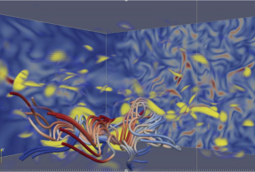
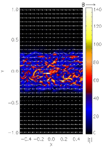
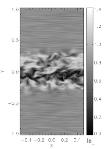
Figure 5: Visualization of reconnection simulations in Kowaletal09 ; Kowaletal12 . Left panel: Magnetic field in the reconnection region. Large perturbations of magnetic field lines arise from reconnection rather than driving; the latter is subAlfvénic. The color corresponds to the polarization of magnetic component $B_{x}$. Central panel: Current intensity and magnetic field configuration during stochastic reconnection. We show a slice through the middle of the computational box in the xy plane after twelve dynamical times for a typical run. The guide field is perpendicular to the page. The intensity and direction of the magnetic field is represented by the length and direction of the arrows. The color bar gives the intensity of the current. The reversal in $B_{x}$ is confined to the vicinity of y=0 but the current sheet is strongly disordered with features that extend far from the zone of reversal. Right panel: Representation of the magnetic field in the reconnection zone with textures.

4.3 Dependence on resistivity, turbulence injection power and turbulence scale

As we show below, simulations in Kowaletal09 ; Kowaletal12 provided very good correspondence to the LV99 analytical predictions for the dependence on resistivity, i.e. no dependence on resistivity for sufficiently strong turbulence driving, and the injection power, i.e. $V_{rec}\sim P_{inj}^{1/2}$. The corresponding dependence is shown in Figure 6.

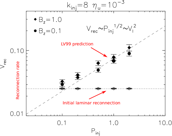
Figure 6: The dependence of the reconnection velocity on the injection power for different simulations with different drivings. The predicted LV99 dependence is also shown. $P_{inj}$ and $k_{inj}$ are the injection power and scale, respectively, $B_{z}$ is the guide field strength, and $\eta_{u}$ the value of unifor resistivity coefficient. From Kowaletal12 .

The measured dependence on the turbulence scale was a bit more shallow compared to the LV99 predictions (see Figure 7). This may be due to the existence of an inverse cascade that changes the driving from the idealized assumptions in LV99 theory.

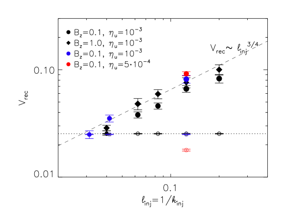
Figure 7: The dependence of the reconnection velocity on the injection scale. From Kowaletal12 .

4.4 Dependence on guide field strength, anomalous resistivity and viscosity

The simulations did not reveal any dependence on the strength of the guide field $B_{z}$ (see Figure 6). This raises an interesting question. In the limit where the parallel wavelength of the strong turbulent eddies is less than the length of the current sheet, we can rewrite the reconnection speed as

$$V_{rec}\approx\left({PL_{x}\over V_{Ax}}\right)^{1/2}{1\over k_{\|}V_{A}}.$$ (25)

Here $P$ is the power in the strong turbulent cascade, $L_{x}$ and $V_{Ax}$ are the length scale and Alfvén velocity in the direction of the reconnecting field, and $V_{A}$ is the total Alfvén velocity, including the guide field. The parallel wavenumber, $k_{\|}$, is characteristic of the large scale strongly turbulent eddies. We have assumed that such eddies are smaller than the size of the current sheet. The point of rewriting the reconnection speed in this way is that it is insensitive to assumptions about the connection between the input power and driving scale and the parameters of the strongly turbulent cascade.

In a physically realistic situation, the dynamics that drive the turbulence, whatever they are, provide a characteristic frequency and input power. Since the guide field enters only in the combination $k_{\|}V_{A}$, i.e. through the eddy turn over rate, this implies that varying the guide field will not change the reconnection speed. However, in the numerical simulations cited above the driving forces are independent of time scale, and sensitive to length scale, so getting the physically realistic scaling is unexpected. Further complicating matters, we note that the dependence on length scale, described in the previous section, is roughly what we expect if $k_{\|}$ is given by the forcing wavenumber.

This is the only clear discrepancy between the simulations and our predictions. It is clearly important to understand its nature. One possibility is that the transfer of energy from the weak turbulence driven by isotropic forcing to the strongly turbulent eddies does not proceed in the expected manner. This may be due to the effect of the strong magnetic shear when a guide field is present. Alternatively, the periodicity of the box, or the possibility that some wave modes may leave the computational box faster than the nonlinear decay rate, may skew the weakly turbulent spectrum. The latter possibilities can be tested by simulating strong turbulence and comparing the results with equation (25). The former will require a more detailed theoretical and computational study of the nature of the strong turbulence in the presence of strong magnetic shear.

The left panel of Figure 8 shows the dependence of the reconnection rate on viscosity. This can be explained as the effect of the finite inertial range of turbulence. For an extended range of motions, LV99 does not predict any viscosity dependence. However, for numerical simulations the range of turbulent motions is very limited and any additional viscosity decreases the resulting velocity dispersion and therefore the field wandering.

LV99 predicted that in the presence of sufficiently strong turbulence, plasma effects should not play a role. The accepted way to simulate plasma effects within MHD code is to use anomalous resistivity. The results of the corresponding simulations are shown in the right panel of Figure 8 and they confirm that the change of the anomalous resistivity does not change the reconnection rate.

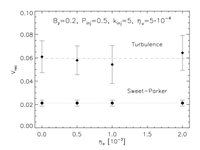
Figure 8: Left panel. The dependence of the reconnection velocity on viscosity. From Kowaletal12 . Right panel. The dependence of reconnection velocity on anomalous resistivity. From Kowaletal09 .

4.5 Structure of the reconnection region

The internal structure of the reconnection region is important, both for the role it plays in determining the overall reconnection speed, and for what it tells us about the nature of local electric currents. We can imagine two extreme pictures. First, the magnetic shear might be concentrated in a narrow, albeit highly distorted sheet, whose width is determined by microphysics. In this case the outflow region would be much broader than the current sheet and particle acceleration would take place in a nearly two dimensional, and highly singular, region. The electric field in the current sheet would be very large, much larger than one would be able to simulate directly. At the other extreme, the current sheet and the outflow zone may roughly coincide. In this case the current sheet is broad and the currents are distributed widely within a three dimensional volume. The electric fields would be roughly similar to what we expect in homogeneous turbulence. In the former case the turbulence within the current sheet is difficult to estimate. In the latter case, it would be similar to the turbulence within a statistically homogeneous volume, of the sort that we can simulate. This would imply that the basic derivation of reconnection speeds in LV99 is valid and particle acceleration takes place in a broad volume. While both of these models are caricatures, they give a good sense of the basic issues at stake.

The structure of the reconnection region was analyzed by Vishniac et al. Vishniacetal12 based on the numerical work by Kowal et al. Kowaletal09 . While this paper only examined simulations with relatively large forcing, the results seem to favour the latter picture, in which the reconnection region is broad, the magnetic shear is more or less coincident with the outflow zone, and the turbulence within it is broadly similar to turbulence in a homogeneous system. In particular, this analysis showed that peaks in the current were distributed throughout the reconnection zone, and that the width of these peaks were not a strong function of their strength. The single best illustration of the results is shown in Figure 9 which shows histograms of magnetic field gradients in the simulations with strong and moderate driving power, with no magnetic field reversal but with driven turbulence, and with no driven turbulence at all, but a passive magnetic field reversal (i.e. Sweet-Parker reconnection). A few features stand out in this figure. First, all the simulations with driven turbulence have a roughly gaussian distribution of magnetic field gradients. In the case with no field reversal (panel c) the peak is narrow and symmetric around zero. In the presence of a large scale field reversal the peak is slightly broadened, and skewed. (The simulation without reconnection was run at a lower resolution, so the total number of cells is smaller by a factor of 8.) Finally, the last panel shows a very spiky distribution of points to the right of the origin. The spikiness is an artifact of the numerical grid. In the absence of turbulence the same values tend to repeat. That occupied bins are all for positive magnetic field gradients is a trivial consequence of the background solution and the laminar nature of Sweet-Parker reconnection.

It is striking that turbulent reconnection does not produce any strong feature corresponding to a preferred value of the magnetic field gradient. Instead one sees a systematic bias towards large positive values. We conclude from the lack of coherent features within the outflow zone, and the broad distribution of values of the gradient of the magnetic field, that the second picture is best. The current sheet and the outflow zone are roughly coincident and this volume is filled with turbulent structures.

One weakness of this analysis is that it has been tested only for relatively strong magnetic turbulence. Although the driven turbulence in these simulations was subalfvenic, they were not very weak. We can expect that the skew in figure 9 will become stronger at as the turbulent velocities are turned down. At some point the mean gradient should begin to affect the turbulent spectrum.

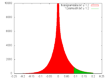
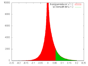
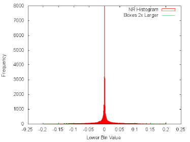
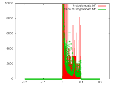
Figure 9: These figures show histograms of the gradient of the reversing component of the large scale magnetic field in the direction normal to the unperturbed current sheet, i.e. $\partial_{y}B_{x}$. Upper left panel is for the highest power simulation, P=1. Upper right panel is for P=0.5. Lower left is for P=1 but with no large scale magnetic field reversal, i.e. simply locally driven strong turbulence. Bins with twice the number of cells as the corresponding bin with the opposite sign of $\partial_{y}B_{x}$ are shown in green. Lower right shows the first simulation in the absence of turbulent forcing. From Vishniacetal12 .

4.6 Testing of magnetic Richardson diffusion

As we discussed, the LV99 model is intrinsically related to the concept of Richardson diffusion in magnetized fluids. Thus by testing the Richardson diffusion of magnetic field, one also provides tests for the theory of turbulent reconnection.

The first numerical tests of Richardson diffusion were related to magnetic field wandering predicted in LV99 Maronetal04 ; Lazarianetal04 ; Beresnyak13a . In Figure 10 we show the results obtained in Lazarianetal04 . There we clearly see different regimes of magnetic field diffusion, including the $y\sim x^{3/2}$ regime. This is a manifestation of the spatial Richardson diffusion.

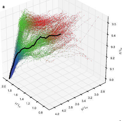
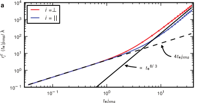
Figure 10: Left panel. Stochastic trajectories that arrive at a fixed point in the archived MHD flow, color-coded redred, greengreen, and blueblue from earlier to later times. From Eyinketal13 . Right panel. Mean-square dispersion of field-lines backwards in time, with redred for direction parallel and blueblue for direction perpendicular to the local magnetic field. From Eyinketal13 .

A direct testing of the temporal Richardson diffusion of magnetic field-lines was performed recently in Eyinketal13 . For this experiment, stochastic fluid trajectories had to be tracked backward in time from a fixed point in order to determine which field lines at earlier times would arrive to that point and be resistively “glued together”. Hence, many time frames of an MHD simulation were stored so that equations for the trajectories could be integrated backward. The results of this study are illustrated in Figure 10. The left panel shows the trajectories of the arriving magnetic field-lines, which are clearly widely dispersed backward in time, more resembling a spreading plume of smoke than a single “frozen-in” line. Quantitative results are presented in the right panel, which plots the root-mean-square line dispersion in directions both parallel and perpendicular to the local mean magnetic field. Times are in units of the resistive time $1/j_{rms}$ determined by the rms current value and distances in units of the resistive length $\lambda/j_{rms}$. The dashed line shows the standard diffusive estimate $4\lambda t,$ while the solid line shows the Richardson-type power-law $t^{8/3}$. Note that this simulation exhibited a $k^{-3/2}$ energy spectrum (or Hölder exponent 1/4) for the velocity and magnetic fields, similar to other MHD simulations at comparable Reynolds numbers, and the self-consistent Richardson scaling is with exponent 8/3 rather 3. Although a $t^{8/3}$ power-law holds both parallel and perpendicular to the local field direction, the prefactor is greater in the parallel direction, due to backreaction of the magnetic field on the flow via the Lorentz force. The implication of these results is that standard diffusive motion of field-lines holds for only a very short time, of order of the resistive time, and is then replaced by super-diffusive, explosive separation by turbulent relative advection. This same effect should occur not only in resistive MHD but whenever there is a long power-law turbulent inertial range. Whatever plasma mechanism of line-slippage holds at scales below the ion gyroradius— electron inertia, pressure anisotropy, etc.—will be accelerated and effectively replaced by the ideal MHD effect of Richardson dispersion.

5 Observational consequences and tests

Historically, studies of reconnection were motivated by observations of Solar flares. There we deal with the collisionless turbulent plasmas and it is important to establish whether plasma microphysics or LV99 turbulent dynamics determine the observed solar reconnection.

Qualitatively, one can argue that there is observational evidence in favor of the LV99 model. For instance, observations of the thick reconnection current outflow regions observed in the Solar flares CiaravellaRaymond08 were predicted within LV99 model at the time when the competing plasma Hall term models were predicting X-point localized reconnection. However, as plasma models have evolved to include tearing and formation of magnetic islands (see Drakeetal10 ) it is necessary to get to a quantitative level to compare the predictions from the competing theories and observations.

To be quantitative one should relate the idealized model LV99 turbulence driving to the turbulence driving within solar flares. In LV99 the turbulence driving was assumed isotropic and homogeneous at a distinct length scale $L_{inj}.$ A general difficulty with observational studies of turbulent reconnection is the determination of $L_{inj}$. One possible approach is based on the the relation $\varepsilon\simeq u_{L}^{4}/V_{A}L_{inj}$ for the weak turbulence energy cascade rate. The mean energy dissipation rate $\varepsilon$ is a source of plasma heating, which can be estimated from observations of electromagnetic radiation (see more in ELV11). However, when the energy is injected from reconnection itself, the cascade is strong and anisotropic from the very beginning. If the driving velocities are sub-Alfvénic, turbulence in such a driving is undergoing a transition from weak to strong at the scale $LM_{A}^{2}$ (see §3.4). The scale of the transition corresponds to the velocity $M_{A}^{2}V_{A}$. If turbulence is driven by magnetic reconnection, one can expect substantial changes of the magnetic field direction corresponding to strong turbulence. Thus it is natural to identify the velocities measured during the reconnection events with the strong MHD turbulence regime. In other words, one can use:

$$V_{rec}\approx U_{obs,turb}(L_{inj}/L_{x})^{1/2},$$ (26)

where $U_{obs,turb}$ is the spectroscopically measured turbulent velocity dispersion. Similarly, the thickness of the reconnection layer should be defined as

$$\Delta\approx L_{x}(U_{obs,turb}/V_{A})(L_{inj}/L_{x})^{1/2}.$$ (27)

Naturally, this is just a different way of presenting LV99 expressions, but taking into account that the driving arises from reconnection and therefore turbulence is strong from the very beginning (see more in Eyinketal13 . The expressions given by Eqs. (26) and (27) can be compared with observations in (CiaravellaRaymond08 ). There, the widths of the reconnection regions were reported in the range from 0.08$L_{x}$ up to 0.16$L_{x}$ while the the observed Doppler velocities in the units of $V_{A}$ were of the order of 0.1. It is easy to see that these values are in a good agreement with the predictions given by Eq. (27). We note, that if we associate the observed velocities with isotropic driving of turbulence, which is unrealistic for the present situation, then a discrepancy with Eq. (27) would appear. Because of that CiaravellaRaymond08 did not get quite as good quantitative agreement between observations and theory as we did, but still within observational uncertainties. In Sychetal09 , authors explaining quasi-periodic pulsations in observed flaring energy releases at an active region above the sunspot, proposed that the wave packets arising from the sunspots can trigger such pulsations. This is exactly what is expected within the LV99 model.

As we discussed in §3.5 the criterion for the application of LV99 theory is that the outflow region is much larger than the ion Larmor radius $\Delta\gg\rho_{i}$. This is definitely satisfied for the solar atmosphere where the ratio of $\Delta$ to $\rho_{i}$ can be larger than $10^{6}$. Plasma effects can play a role for small scale reconnection events within the layer, since the dissipation length based on Spitzer resistivity is $\sim 1$ cm, whereas $\rho_{i}\sim 10^{3}$ cm (Table LABEL:tab:parameters). However, as we discussed earlier, this does not change the overall dynamics of turbulent reconnection.

Reconnection throughout most of the heliosphere appears similar to that in the Sun. For example, there are now extensive observations of reconnection jets (outflows, exhausts) and strong current sheets in the solar wind Gosling12 . The most intense current sheets observed in the solar wind are very often not observed to be associated with strong (Alfvénic) outflows and have widths at most a few tens of the proton inertial length $\delta_{i}$ or proton gyroradius $\rho_{i}$ (whichever is larger). Small-scale current sheets of this sort that do exhibit observable reconnection have exhausts with widths at most a few hundreds of ion inertial lengths and frequently have small shear angles (strong guide fields) Goslingetal07 ; GoslingSzabo08 . Such small-scale reconnection in the solar wind requires collisionless physics for its description, but the observations are exactly what would be expected of small-scale reconnection in MHD turbulence of a collisionless plasma Vasquezetal07 . Indeed, LV99 predicted that the small-scale reconnection in MHD turbulence should be similar to large-scale reconnection, but with nearly parallel magnetic field lines and with “outflows” of the same order as the local, shear-Alfvénic turbulent eddy motions. It is worth emphasizing that reconnection in the sense of flux-freezing violation and disconnection of plasma and magnetic fields is required at every point in a turbulent flow, not only near the most intense current sheets. Otherwise fluid motions would be halted by the turbulent tangling of frozen-in magnetic field lines. However, except at sporadic strong current sheets, this ubiquitous small-scale turbulent reconnection has none of the observable characteristics usually attributed to reconnection, e.g. exhausts stronger than background velocities, and would be overlooked in observational studies which focus on such features alone.

However, there is also a prevalence of very large-scale reconnection events in the solar wind, quite often associated with interplanetary coronal mass ejections and magnetic clouds or occasionally magnetic disconnection events at the heliospheric current sheet Phanetal09 ; Gosling12 . These events have reconnection outflows with widths up to nearly $10^{5}$ of the ion inertial length and appear to be in a prolonged, quasi-stationary regime with reconnection lasting for several hours. Such large-scale reconnection is as predicted by the LV99 theory when very large flux-structures with oppositely-directed components of magnetic field impinge upon each other in the turbulent environment of the solar wind. The “current sheet” producing such large-scale reconnection in the LV99 theory contains itself many ion-scale, intense current sheets embedded in a diffuse turbulent background of weaker (but still substantial) current. Observational efforts addressed to proving/disproving the LV99 theory should note that it is this broad zone of more diffuse current, not the sporadic strong sheets, which is responsible for large-scale turbulent reconnection. Note that the study Eyinketal13 showed that standard magnetic flux-freezing is violated at general points in turbulent MHD, not just at the most intense, sparsely distributed sheets. Thus, large-scale reconnection in the solar wind is a very promising area for LV99. The situation for LV99 generally gets better with increasing distance from the sun, because of the great increase in scales. For example, reconnecting flux structures in the inner heliosheath could have sizes up to $\sim$100 AU, much larger than the ion cyclotron radius $\sim 10^{3}$ km LazarianOpher09 .

The magnetosphere is another example that is under active investigation by the reconnection community. The situation there is different, as $\Delta\sim\rho_{i}$ is the general rule and we expect plasma effects to be dominant. Turbulence of whistler waves, e.g. electron MHD (EMHD) turbulence may play its role, however. For instance, Huangetal12 reported a magnetotail event in which they claim that turbulent electromotive force is responsible for reconnection. The turbulence at those scales is not MHD. We may speculate that the LV99 can be generalized for the case of EMHD and apply to such events. This should be the issue of further studies.

It may be worth noting that the possibility of in-situ measurements of magnetospheric reconnection make it a very attractive subject for the reconnection community. Upcoming missions like the Magnetospheric Multiscale Mission (MMS), set to launch in 2014, will provide detailed observations of reconnection diffusion regions, energetic particle acceleration, and micro-turbulence in the magnetospheric plasma. In addition to the exciting prospect of better understanding of the near-Earth space environment, the hope has been expressed that this mission will provide insight into magnetic reconnection in a very wide variety of astrophysical and terrestial plasmas. We believe that magnetospheric observations may indeed shed light on magnetic reconnection in man-made settings such as fusion machines (tokamaks or spheromaks) and laboratory reconnection experiments, which also involve collisionless plasmas and overall small length scales. However, magnetospheric reconnection is a rather special, non-generic case in astrophysics, with $\Delta$ of the order or less than $\rho_{i}$, while the larger scales involved in most astrophysical processes imply that $\Delta\gg\rho_{i}$. We claim that this is the domain where turbulence and the broadening of $\Delta$ that it entails must be accounted for. Thus, magnetospheric reconnection, in the opinion of the present reviewers, is a special case which will provide insight mainly into micro-scale aspects of reconnection, which are of more limited interest in general astrophysical environments. Reconnection elsewhere in the solar system, including the sun, its atmosphere, and the larger heliosphere (solar wind, heliosheath, etc.) are better natural laboratories for observational study of generic astrophysical reconnection in both collisionless and collisional environments.

6 Extending LV99 theory

6.1 Reconnection in partially ionized gas

Turbulence in the partially ionized gas is different from that in fully ionized plasmas. One of the critical differences arises from the viscosity caused by neutrals atoms. This results in the media viscosity being substantially larger than the media resistivity. The ratio of the former to the latter is called the Prandtl number and in what follows we consider high Prandtl number turbulence. In reality, MHD turbulence in the partially ionized gas is more complicated as decoupling of ions and neutrals and other complicated effects occur at sufficiently small scale. The discussion of these regimes is given in Lazarianetal04 . However, for the purposes of reconnection, we believe that a simplified discussion below is adequate, as follows from the fact that we discussed earlier, namely, that the LV99 reconnection is determined by the dynamics of large scales of turbulent motions.

The high Prandtl number turbulence was studied numerically in Choetal02 ; Choetal03 ; SchekochihinCowley04 and theoretically in Lazarianetal04 . What is important for our present discussion is that for scales larger than the viscous damping scale the turbulence follows the usual GS95 scaling, while it develops a shallow power law magnetic tail and steep velocity spectrum below the viscous damping scale $\ell_{\perp,crit}$. The existence of the GS95 scaling at sufficiently large scales means that our considerations about Richardson diffusion and magnetic reconnection that accompany it should be valid at these scales. Thus, our goal is to establish the scale of current sheets starting from where the Richardson diffusion will induce the accelerated separation of magnetic field lines.

In high Prandtl number media the GS95-type turbulent motions decay at the scale $l_{\bot,crit}$, which is much larger than the scale at which Ohmic dissipation becomes important. Thus over a range of scales less than $l_{\bot,crit}$ to some much smaller scale magnetic field lines preserve their identity. These magnetic field lines are being affected by the shear on the scale $l_{\bot,crit}$, which induces a new regime of turbulence described in Choetal02 and Lazarianetal04 .

To establish the range of scales at which magnetic fields perform Richardson diffusion one can observe that the transition to the Richardson diffusion is expected to happen when field lines get separated by the perpendicular scale of the critically damped eddies $l_{\bot,crit}$. The separation in the perpendicular direction starts with the scale $r_{init}$ following the Lyapunov exponential growth with the distance $l$ measured along the magnetic field lines, i.e. $r_{init}\exp(l/l_{\|,crit})$, where $l_{\|,crit}$ corresponds to critically damped eddies with $l_{\perp,crit}$. It seems natural to associate $r_{init}$ with the separation of the field lines arising from the action of Ohmic resistivity on the scale of the critically damped eddies

$$r_{init}^{2}=\eta l_{\|,crit}/V_{A},$$ (28)

where $\eta$ is the Ohmic resistivity coefficient.

The problem of magnetic line separation in turbulent fluids was considered for chaotic separation in smooth, laminar flows by Rechester & Rosenbluth RechesterRosenbluth78 and for superdiffusive separation in turbulent plasmas by Lazarian Lazarian06 . Following the logic in the paper and taking into account that the largest shear arises from the critically damped eddies, it is possible to determine the distance to be covered along magnetic field lines before the lines separate by the distance larger than the perpendicular scale of viscously damped eddies is equal to

$$L_{RR}\approx l_{\|,crit}\ln(l_{\bot,crit}/r_{init})$$ (29)

Taking into account Eq. (28) and that

$$l_{\bot,crit}^{2}=\nu l_{\|,crit}/V_{A},$$ (30)

where $\nu$ is the viscosity coefficient. Thus Eq. (29) can be rewritten

$$L_{RR}\approx l_{\|,crit}\ln Pt$$ (31)

where $Pt=\nu/\eta$ is the Prandtl number.

If the current sheets are much longer than $L_{RR}$, then magnetic field lines undergo Richardson diffusion and according to Eyinketal11 the reconnection follows the laws established in LV99. In other words, on scales significantly larger than the viscous damping scale LV99 reconnection is applicable. At the same time on scales less than $L_{RR}$ magnetic reconnection may be slow. This small scale reconnection regime requires further studies. For instance, results of laminar reconnection in the partially ionized gas obtained analytically in VishniacLazarian99 and studied numerically by HeitschZweibel03 can be applicable. This approach has been recently used by Leakeetal12 to explain chromospheric reconnection that takes place in weakly ionized plasmas. In this review we, however, are interested at reconnection at large scales and therefore do not dwell on small scale phenomena.

For the detailed structure of the reconnection region in the partially ionized gas the study in Lazarianetal04 is relevant. There the magnetic turbulence below the scale of the viscous dissipation is accounted for. However, those magnetic structures on the small scales cannot change the overall reconnection velocities.

6.2 Development of turbulence due to magnetic reconnection

Astrophysical fluids are generically turbulent. However, even if the initial magnetic field configuration is laminar, magnetic reconnection ought to induce turbulence due to the outflow (LV99, LazarianVishniac09 ). This effect was confirmed by observing the development of turbulence both in recent 3D Particle in Cell (PIC) simulations (Karimabadietal13 ) and 3D MHD simulations (Beresnyak13b ; Kowaletal13 ).

Earlier on, the development of chaotic structures due to tearing was reported in Loureiroetal09 as well as in subsequent publications (see Bhattacharjeeetal09 ). However, we should stress that there is a significant difference between turbulence development in 2D and 3D simulations. As we discussed in §3.2 the very nature of turbulence is different in 2D and 3D. In addition, the effect of the outflow is very different in simulations with different dimentionality. For instance, in 2D the development of the Kelvin-Hemholtz instability is suppressed by the field that is inevitably directed parallel to the outflow. On the contrary, the outflow can induce this instability in the generic 3D configuration. In general, we do expect realistic 3D systems to be more unstable and therefore prone to development of turbulence. This corresponds well to the results of 3D simulations that we refer to.

Beresnyak Beresnyak13b studied the properties of reconnection-driven turbulence and found its correspondence to those expected for MHD turbulence (see §3.2). The difference with isotropically driven turbulence is that magnetic energy is observed to be dominant compared with kinetic energy. The periodic boundary conditions adopted in Beresnyak13b limits the time span over which magnetic reconnection can be studied and therefore the simulations focus on the process of establishing reconnection. Nevertheless, as the simulations reveal a nice turbulence power law behavior, one can apply the approach of turbulent reconnection and closely connected to it, Richardson diffusion (see §3.4).

Beresnyak (2013, private communication) used LV99 approach and obtained expressions describing the evolution of the reconnection layer in the transient regime of turbulence development that he observes. Below we provide our theoretical account of the results in Beresnyak13b using our understanding of turbulent reconnection also based on LV99 theory. However, we get expressions which differ from those by Beresnyak.

The logic of our derivation is really simple. As the magnetic fluxes get into contact the width of the reconnection layer $\Delta$ is growing. The rate at which this happens is limited by the mixing rate induced by the eddies at the scale $\Delta$, i.e.

$$\frac{1}{\Delta}\frac{d\Delta}{dt}\approx g\frac{V_{\Delta}}{\Delta}$$ (32)

with a factor $g$ which takes into account possible inefficiency in the diffusion process. As $V_{\Delta}$ is a part of the turbulent cascade, i.e. the mean value of $V_{\Delta}^{2}\approx\int\Phi(k_{1})dk_{1}$, where

$$\Phi=C_{k}\epsilon^{2/3}k^{-5/3}_{1},$$ (33)

and $C_{k}$ is a Kolmogorov constant, which for ordinary MHD turbulence is calculated in Beresnyak12 , but in our special case may be different. If the energy dissipation rate $\varepsilon$ were time-independent, then the layer width would be implied by Eqs. (32) and (33) to grow according to Richardson’s law $\Delta^{2}\sim\varepsilon t^{3}.$ However, in the transient regime considered, energy dissipation rate is evolving. If the y-component of the magnetic field is reconnecting and the cascade is strong, then the mean value of the dissipation rate $\epsilon$ is

$$\epsilon\approx\beta V_{Ay}^{2}/(\Delta/V_{\Delta}),$$ (34)

where $\beta$ is another coefficient measuring the efficiency of conversion of mean magnetic energy into turbulent fluctuations. This coefficient can be obtained from numerical simulations.

The ability of the cascade to be strong from the very beginning follows from the large perturbations of the magnetic fields by magnetic reconnection, while magnetic energy can still dominate the kinetic energy. The latter factor that can be experimentally measured is given by a parameter $r_{A}$. With this factor and making use of Eqs.(33) and (34), the expression for $V_{\Delta}$ can be rewritten in the following way:

$$V_{\Delta}\approx C_{k}r_{A}(V_{Ay}^{2}V_{\Delta}\beta)^{2/3}$$ (35)

where the dependences on $k_{1}\sim 1/\Delta$ cancel out.

This provides the expression for the turbulent velocity at the injection scale $V_{\Delta}$

$$V_{\Delta}\approx(C_{K}r_{A})^{3/4}V_{Ay}\beta^{1/2}$$ (36)

as a function of the experimentally measurable parameters of the system. Thus the growth of the turbulent reconnection zone is according to Eq.(32)

$$\frac{d\Delta}{dt}\approx g\beta^{1/2}(C_{K}r_{A})^{3/4}V_{Ay}$$ (37)

which predicts the nearly constant growth of the outflow region as seen in Fig.3 in Beresnyak13b .

Using the values of the numerical constants provided to us by Beresnayk we get a fair correspondence with the results of simulations in Beresnyak13b . However, we feel that further testings are necessary.

As the reconnection gets into the steady state regime, one expects the outflow to play an important role and therefore the reconnection rate gets modified. This regime cannot be studied in periodic box simulations like those in Beresnyak13b as they require studies for more than one Alfven crossing time. Studies with open boundary conditions are illustrated by Figure 11 from our new study.

The equations for the reconnection rate were obtained in LV99 for the isotropic injection of energy. For the case of anisotropic energy injection of turbulence we should apply the approach in § 5. Using Eq. (27) and identifying $V_{\Delta}$ with the total velocity dispersion, which is similar to the use of $U_{obs,turb}$ in Eq. (26) one can get

$$V_{rec}\approx V_{\Delta}(\Delta/L_{x})^{1/2}$$ (38)

where the mass conservation condition provides the relation $V_{rec}L_{x}\approx V_{Ay}\Delta$. Using the latter condition one gets

$$V_{rec}\approx V_{Ay}(C_{K}r_{A})^{3/2}\beta$$ (39)

which somewhat slower than the rate at which the reconnection layer was growing initially. The latter behavior of reconnection is also present for the Sweet-Parker reconnection, since the reconnection rate can be faster even before the formation of steady state current sheet (see Kowaletal09 ).

We are going to compare the prediction given by Eq. (LABEL:ref_self) against the results of recent simulations illustrated by Figure 11. The figure shows a few slices of the magnetic field strength $|\vec{B}|$ through the three-dimensional computational domain with dimensions $L_{x}=1.0$ and $L_{y}=L_{z}=0.25$. The simulation was done with the resolution $2048\times 512\times 512$. Open boundary conditions along the X and Y directions allowed studies of steady state turbulence. At the presented time $t=1.0$ the turbulence strength increased by two orders of magnitude from its initial value of $E_{kin}\approx 10^{-4}E_{mag}$. Initially, only the seed velocity field at the smallest scales was imposed (a random velocity vector was set for each cell). We expect that most of the injected energy comes from the Kelvin-Helmholtz instability induced by the local interactions between the reconnection events, which dominates in the Z-direction, along which a weak guide field is imposed ($B_{z}=0.1B_{x}$). As seen in the planes perpendicular to $B_{x}$ in Figure 11, Kelvin-Helmholtz-like structures are already well developed at time $t=1.0$. Turbulent structures are also observed within the XY-plane, which probably are generated by the strong interations of the ejected plasma from the neighboring reconnection events. More detailed analysis of the spectra of turbulence and efficiency of the Kelvin-Helmholtz instability as the turbulent injection mechanism are presented in Kowaletal13 .

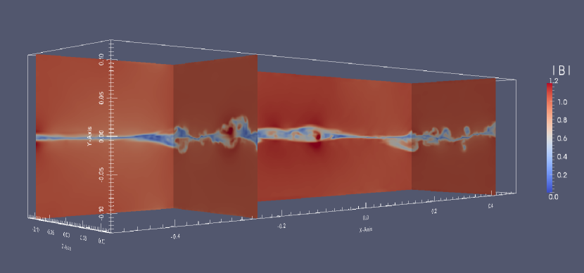
Figure 11: Visualization of the model of turbulence generated by the seed reconnection from Kowaletal13 . Three different cuts (one XY plane at Z=-0.1 and two YZ-planes at X=-0.25 and X=0.42) through the computational domain show the strength of magnetic field $|\vec{B}|$ at the evolution time $t=1.0$. Kelvin-Helmholtz-type structures are well seen in the planes perpendicular to the reconnecting magnetic component $B_{x}$. In the Z direction, the Kelvin-Helmholtz instability is slightly suppressed by the guide field of the strength $B_{z}=0.1B_{x}$ (with $B_{x}=1.0$ initially). The initial current sheet is located along the XZ plane at Y=0.0. A weak ($E_{kin}\approx 10^{-4}E_{mag}$) random velocity field was imposed initialy in order to seed the reconnection.

6.3 Effect of energy dissipation in the reconnection layer

In the original LV99 paper it was argued that only a small fraction of the energy stored in the magnetic field is lost during large-scale reconnection and the magnetic energy is instead converted nearly losslessly to kinetic energy of the outflow. This can only be true, however, when the Alfvénic Mach number $M_{A}=u_{L}/V_{A}$ is small enough. If $M_{A}$ becomes too large, then it was argued in ELV11 that energy dissipation in the reconnection layer becomes non-negligible compared to the available magnetic energy and there is a consequent reduction of the outflow velocity. Note that even if $M_{A}$ is initially small, reconnection may drive stronger turbulence (see previous subsection) and increase the fluctuation velocities $u_{L}$ in the reconnection layer. This scenario may be relevant to post-CME reconnection, for example, where there is empirical evidence that the energy required to heat the plasma in the reconnection layer (“current sheet”) to the observed high temperatures is from energy cascade due to turbulence generated by the reconnection itself Susinoetal13 . In addition, $V_{A}$ within the reconnection layer will be smaller than the upstream values, because of annihilation of the anti-parallel components, which will further increase the Alfvénic Mach number. If $M_{A}$ rises to a sufficiently large value, then the energy dissipated becomes large enough to cause a reduction in the outflow velocity $v_{out}$ below the value $V_{A}$ assumed in LV99 and the predictions of the theory must be modified. We consider here briefly the modification proposed in ELV11 and some of its consequences.

The effect of turbulent dissipation can be estimated from steady-state energy balance in the reconnection layer:

$$\frac{1}{2}v_{out}^{3}\Delta=\frac{1}{2}V_{A}^{2}v_{ren}L_{x}-\varepsilon L_{x}\Delta,$$ (40)

where kinetic energy carried away in the outflow is balanced against magnetic energy transported into the layer minus the energy dissipated by turbulence. Here we estimate the turbulent dissipation using the formula $\varepsilon=u_{L}^{4}/V_{A}L_{i}$ for sub-Alfvénic turbulence Kraichnan65 . If one divides (40) by $\Delta=L_{x}v_{rec}/v_{out}$, one gets

$$v_{out}^{3}=V_{A}^{2}v_{out}-2\frac{u_{L}^{4}}{V_{A}}\frac{L_{x}}{L_{i}},$$ (41)

which is a cubic polynomial for $v_{out}$. The solutions are easiest to obtain by introducing the ratios $f=v_{out}/V_{A}$ and $r=2M_{A}^{4}(L_{x}/L_{i})$ which measure, respectively, the outflow speed as a fraction of $V_{A}$ and the energy dissipated by turbulence in units of the available magnetic energy, giving

$$r=f-f^{3}.$$ (42)

When $r=0$, the only solution of (42) with $f>0$ is $f=1,$ recovering the LV99 estimate $v_{out}=V_{A}$ for $M_{A}\ll 1.$ For somewhat larger values of $r,$ $f\simeq 1-(r/2)$, in agreement with the formula $f=(1-r)^{1/2}$ that follows from eq.(65) in ELV11, implying a slight decrease in $v_{out}$ compared with $V_{A}.$ Note that formula (42) cannot be used to determine $f$ for too large $r$, because it has then no positive, real solutions! This is easiest to see by considering the graph of $r$ vs. $f$. The largest value of $r$ for which a positive, real $f$ exists is $r_{max}=2/\sqrt{27}\approx 0.385$ and then $f$ takes on its minimum value $f_{min}=1/\sqrt{3}\approx 0.577$. This implies that the LV99 approach is limited to $M_{A}$ sufficiently small, because of the energy dissipation inside the reconnection layer and the consequent reduction of the outflow velocity. This is not a very stringent limitation, however, because $r$ is proportional to $M_{A}^{4}$. If one assumes $L_{x}\simeq L_{i}$, one may consider values of $M_{A}$ up to $0.662$. Given the neglect of constants of order unity in the above estimate, we may say only that the LV99 approach is limited to $M_{A}\lesssim 1.$ At the extreme limit of applicability of LV99, $v_{out}$ is still a sizable fraction of $V_{A}$, i.e. 0.577, not a drastically smaller value.

The effect of the reduced outflow velocity may be, somewhat paradoxically, to increase the reconnection rate. The reason is that field-lines now spend a time $L_{x}/v_{out}$ exiting from the reconnection layer, greater than assumed in LV99 by a factor of $1/f.$ This implies a thicker reconnection layer $\Delta$ due to the longer time-interval of Richardson diffusion in the layer, greater than LV99 by a factor of $(1/f)^{3/2}.$ The net reconnection speed $v_{rec}=v_{out}\Delta/L_{x}$ is thus larger by a factor of $(1/f)^{1/2}.$ The increased width $\Delta$ more than offsets the reduced outflow velocity $v_{out}.$ However, this effect can give only a very slight increase, at most by a factor of $3^{1/4}\simeq 1.31$ for $f_{min}=1/\sqrt{3}.$ We see that for the entire regime $M_{A}\lesssim 1$ where LV99 theory is applicable, energy dissipation in the reconnection layer implies only very modest corrections. It is worth emphasizing that “large-scale reconnection” in super-Alfvénic turbulence with $M_{A}>1$ is a very different phenomenon, because magnetic fields are then so weak that they are easily bent and twisted by the turbulence. Any large-scale flux tubes initially present will be diffused by the turbulence through a process much different than that considered by LV99. For a discussion of this regime, see KimDiamond01 .

6.4 Relativistic reconnection

Magnetic turbulence in a number of astrophysical highly magnetized objects, accretion disks near black holes, pulsars, gamma ray bursts may be in the relativistic regime when the Alfvén velocity approaches that of light. The equations that govern magnetized fluid in this case look very different from the ordinary MHD equations. However, studies by Cho05 and ChoLazarian13 show that for both balanced and imbalanced turbulence, the turbulence spectrum and turbulence anisotropies are quite similar in this regime and the non-relativistic one. This suggests that the Richardson diffusion and related processes of LV99-type magnetic reconnection should cary on to the relativistic case (see Lazarian & Yan 2012). This prediction was confirmed by the recent numerical simulations Makoto Takomoto (2014, private communication) who with his relativistic code adopted the approach in Kowal et al (2009) and showed that the rate of 3D relativistic magnetic reconnection gets independent of resistivity.

The suggestion that LV99 is applicable to relativistic reconnection motivated the use of the model for explaining gamma ray bursts in Lazarianetal03 and ZhangYan11 studies (see also §7.2) and in accretion disks around black holes and pulsars studies deGouveiadalPinoLazarian05 ; Giannios13 . Now, as the extension of the model to relativistic case has be confirmed these and other cases where the relativistic analog of LV99 process was discussed to be applicable (see Lyutikov & Lazarian 2013) are given numerical support.

Naturally, more detailed studies of both relativistic MHD turbulence and relativistic magnetic reconnection are required (see also chapter by de Gouveia Dal Pino and Kowal in this volume and references therein). It is evident that in magnetically-dominated, low-viscous plasmas turbulence is a generic ingredient and thus it must be taken into account for relativistic magnetic reconnection. As we discuss elsewhere in the review the driving of turbulence may by external forcing or it can be driven by reconnection itself.

7 Implications of fast reconnection in turbulent fluids

7.1 Flux freezing in astrophysical fluids

Since the concept was first proposed by Hannes Alfvén in 1942, the principle of frozen-in field lines has provided a powerful heuristic which allows simple, back-of-the-envelope estimates in place of full solutions (analytical or numerical) of the MHD equations (Parker79 , Kulsrud05 ). As such, the flux-freezing principle has been applied to gain insight into diverse processes, such as star formation, stellar collapse, magnetic dynamo, solar wind magnetospheric interactions, etc. However, it has long been understood that magnetic flux-conservation, if strictly valid, would forbid magnetic reconnection, because field-lines frozen into a continuous plasma flow cannot change their topology. Thus, the flux-freezing principle is in apparent contradiction with numerous observations of fast reconnection in high-conductivity plasmas.

Quite apart from these serious empirical difficulties, the flux-freezing principle has recently been shaken by a fundamental theoretical problem. Standard mathematical proofs of flux-freezing in MHD always assume, implicitly, that velocity and magnetic fields remain smooth as $\eta\rightarrow 0$. However, MHD solutions with small resistivities and viscosities (high magnetic and kinetic Reynolds numbers) are generally turbulent. These solutions exhibit long ranges of power-law spectra corresponding to very non-smooth or “rough” magnetic and velocity fields. Fluid particle (Lagrangian) trajectories in such rough flows are known to be non-unique and stochastic (see Bernardetal98 ; GawedzkiVergassola00 ; EEijnden00a ; EEijnden00b ; EEijnden01 ; Chavesetal03 , and, for reviews, Kupiainen03 and Gawedzki08 ). In fact, it is possible to show that, in the limit of infinite Reynolds number, there is an infinite random ensemble of particle motions for the same initial conditions! This remarkable phenomenon has been called spontaneous stochasticity. It view of the above, it is immediately clear as a consequence that standard flux-freezing cannot hold in turbulent plasma flows. After all, the usual idea is that magnetic field-lines at high conductivity are tied to the plasma flow and follow the fluid motion. However, if the latter is non-unique and stochastic, then which fluid element will the field-line follow?

The phenomenon of spontaneous stochasticity in magnetic field was shown to be inseparably related to LV99 reconnection theory in ELV11. It provides, however, a new outlook on the problem of magnetic field in turbulent fluids. The notion of the violation of the flux conservation Alfvén theorem is implicit in LV99 (but it is expressed explicitly in VishniacLazarian99 ). At the moment we can definitively assert that the domain of the Alfvén theorem on flux freezing is limited to laminar fluids only.

In view of the longstanding misconceptions about the general validity of magnetic flux-conservation for high-conductivity MHD, it is worth making a few more detailed remarks. The standard textbook proofs of flux-conservation (e.g. Chandrasekhar61 ) all make implicit assumptions that are violated in turbulent flow. The proofs typically start with the ideal induction equation

$$\partial_{t}{\bf B}=\nabla\times({\bf u}\times{\bf B})$$

and consider a material surface $S(t)$ advected by velocity ${\bf u}$. Then the time-derivative of the flux integral becomes

$$\frac{d}{dt}\int_{S(t)}{\bf B}(t)\cdot d{\bf A}=\int_{S(t)}\partial_{t}{\bf B}(t)\cdot d{\bf A}+\int_{C(t)}{\bf B}(t)\cdot({\bf u}\times d{\bf x}).$$

The first term from the evolution of ${\bf B}$ and the second term from the motion of the surface cancel identically, implying constant flux through the surface. Of course, in reality, there is always a finite conductivity $\sigma$, however large, and the induction equation is

$$\partial_{t}{\bf B}=\nabla\times({\bf u}\times{\bf B})+\lambda\triangle{\bf B},$$

with $\lambda=c^{2}/4\pi\sigma$. The last term represents a diffusion of magnetic field lines in or out of the surface element, so that flux is no longer exactly conserved.

For a laminar velocity field, this diffusion effect is small. It is not hard to see that a pair of field lines will attain a displacement ${\bf r}(t)$ apart under the combined effect of advection and diffusion obeying

$$\frac{d}{dt}\langle r^{2}\rangle=12\lambda+2\langle{\bf r}\cdot\delta{\bf u}({\bf r})\rangle$$

where $\delta{\bf u}({\bf r})$ is the relative advection velocity at separation ${\bf r}$. Thus,

$$\frac{d}{dt}\langle r^{2}\rangle\leq 12\lambda+2\|\nabla{\bf u}\|\langle r^{2}\rangle,$$

where $\|\nabla{\bf u}\|$ is the maximum value of the velocity-gradient $\nabla{\bf u}$. It follows that two lines initially at the same point, by time $t$ can have separated at most

$$\langle r^{2}(t)\rangle\leq 6\lambda\frac{e^{2\|\nabla{\bf u}\|t}-1}{\|\nabla{\bf u}\|}.$$ (43)

If we thus consider a smooth laminar flow with a fixed, finite value of $\|\nabla{\bf u}\|$, then $\langle r^{2}(t)\rangle\rightarrow 0$ as $\lambda\rightarrow 0$. Under such an assumption, magnetic field lines do not diffuse a far distance away from the solution of the deterministic ordinary differential equation $d{\bf x}/dt={\bf u}({\bf x},t)$, and the magnetic line-diffusion becomes a negligible effect. In that case, magnetic flux is conserved better as $\lambda$ decreases.

However, in a turbulent flow, the above argument fails! The inequality (43) still holds, of course, but it no longer restricts the dispersion of field-lines under the joint action of resistivity and advection. As is well-known, a longer and longer inertial range of power-law spectrum $E(k)$ occurs as viscosity $\nu$ decreases and the maximum velocity gradient $\|\nabla{\bf u}\|$ becomes larger and larger. In fact, energy dissipation $\varepsilon=\nu\|\nabla{\bf u}\|^{2}$ is observed to be non-vanishing as $\nu\rightarrow 0$ in turbulent flow, requiring velocity gradients to grow unboundedly. Estimating $\|\nabla{\bf u}\|\sim(\varepsilon/\nu)^{1/2}$, the upper bound (43) becomes

$$\langle r^{2}(t)\rangle\leq 6\lambda(\nu/\varepsilon)^{1/2}[\exp(2t(\varepsilon/\nu)^{1/2})-1].$$ (44)

This bound allows unlimited diffusion of field-lines. Consider first the case $\lambda=\nu$ or $Pt=1$, for simplicity, where Richardson’s theory implies that

$$\langle r^{2}(t)\rangle\sim 12\lambda t+\varepsilon t^{3}.$$ (45)

The rigorous upper bound always lies strictly above Richardson’s prediction and, in fact, goes to infinity as $\nu=\lambda\rightarrow 0$! The case of large Prandtl number is just slightly more complicated, as previously discussed in §6.1. When $Pt\gg 1,$ the inequality (44) holds as an equality for times $t\ll t_{trans}$ with

$$t_{trans}=\frac{\ln(Pt)}{2(\varepsilon/\nu)}.$$ (46)

This is then followed by a Richardson diffusion regime

$$\langle r^{2}(t)\rangle\sim 6(\nu^{3}/\varepsilon)^{1/2}+\varepsilon(t-t_{trans})^{3},\,\,\,\,\,\,\,\,\,\,\,\,\,\,\,\,t\gg t_{trans},$$ (47)

assuming that the kinetic Reynolds number is also large and a Kolmogorov inertial range exists at scales greater than the Kolmogorov length $(\nu^{3}/\varepsilon)^{1/4}.$ Once again, the upper bound (44) is much larger than Richardson’s prediction and, at times longer than $t_{trans},$ the dispersion of field lines is independent of resistivity.

The textbook proofs of magnetic flux-freezing for ideal MHD are therefore based on unstated assumptions which are explicitly violated in turbulent flows. They are mathematically valid derivations with appropriate assumptions, but physically inapplicable in typical astrophysical systems with plasma turbulence at MHD scales. It is worth emphasizing that any attempt to obtain fast reconnection (independent of resistivity) within a similar hydromagnetic description must likewise account for flux-freezing violation. For example, it has been conjectured Mandtetal94 ; ShayDrake98 that reconnection rates are independent of resistivity in Hall MHD X-point reconnection. This proposal faces the same a priori theoretical difficulty as MHD-based theories, since magnetic field-lines remain frozen-in to the electron fluid in ideal Hall MHD. The conjectured failure of flux-freezing in Hall MHD X-point reconnection even as $\lambda\rightarrow 0$ must therefore be explained. Analytical studies of Hall reconnection indicate that the mechanism may be mathematically similar to the turbulent LV99 case, in that gradients of the electron fluid velocity ${\bf u}^{e}$ in the direction of the outgoing reconnection jets are predicted to diverge proportional to $S,$ the Lundquist number Malyshkin08 ; Shivamoggi11 .

The Hall effects discussed above, as well as other microscopic plasma effects, are not expected to modify the Richardson diffusion of magnetic field lines at length scales much greater than the ion Larmor radius (see Appendix B of ELV11 and section 3.5 of this review). However, one may worry that additional hydrodynamic effects at large scales may fundamentally alter Richardson diffusion. For example, in the Kraichnan-Kazantsev turbulence model Kraichnan65 , where “spontaneous stochasticity” was first predicted, it was shown that a sufficiently high degree of compressibility may eliminate Richardson dispersion entirely and replace it with instead a coalescence of fluid particles GawedzkiVergassola00 ; EvandenEijnden01 . If such effects were found in compressible MHD turbulence, then they could strongly alter the quantitative predictions of LV99, at the very least. This is a particular source of concern because most astrophysical plasmas are compressible, with Mach numbers ranging from a bit less than unity (subsonic) to very large (hypersonic). Note that the numerical tests of Richardson dispersion reported in section 4.6 were for incompressible MHD turbulence. Could compressible MHD turbulence be fundamentally different?

There is at this time no complete theory of Richardson dispersion for MHD turbulence (or, for that matter, for hydrodynamic turbulence), but there are several reasons to believe that compressibility effects will be minimal on the turbulent motion of field lines relevant to reconnection. First, very high degrees of compressibility are required in the Kraichnan model Kraichnan65 to eliminate spontaneous stochasticity. In 3D the kinetic energy in the potential part of the flow must be 10 times greater than in the solenoidal part! Such extreme compressibility is rare in astrophysics. Of course, the Kraichnan model velocity is Gaussian and contains no compressible coherent structures like shocks, which may magnify the compressibility effects. It is well-known that the simple Burgers model, which is entirely potential flow, exhibits no spontaneous stochasticity but instead coalescence of particles in shocks BauerBernard99 . However, Burgers differs in another crucial respect from the Kraichnan model in that it is time-irreversible. As discussed in Eyink11 and ELV11, it is the Richardson dispersion of magnetic field lines backward in time which is relevant to breakdown of flux-freezing. As shown in Eyinketal13 , the Burgers model does exhibit spontaneous stochasticity backward in time and field lines will thus not be “frozen-in” for vanishing resistivities. This is completely unlike the Kraichnan model for pure potential flow in which fluid particles coalesce backward in time as well as forward. In the Burgers model, therefore, magnetic field lines which arrive together at the shock become glued together to produce a resultant magnetic field at the shock. This is the same thing that happens at each point in incompressible MHD turbulence! Our second argument is thus that micro-scale shocklets in compressible MHD turbulence will probably glue field lines together in a manner almost indistinguishable from the surrounding “sea” of rough turbulence with continuous velocities. Finally, we note that the compressible MHD wave modes (slow and fast magnetosonic waves) are found in numerical simulations to decouple dynamically from the solenoidal shear-Alfvén modes, which exhibit turbulence characteristics very similar to those of incompressible MHD ChoLazarian02 ; ChoLazarian03 . Since shear-Alfvén waves produce the dominant fluid motions normal to the direction of the mean magnetic field, they will be the principal drivers of magnetic field-line diffusion across a turbulent reconnection layer. While more research into compressible MHD turbulence is desirable, the above facts support the view that compressibility effects will not strongly alter turbulent magnetic reconnection.

7.2 Solar flares and gamma ray bursts

Preexisting turbulence is a rule for astrophysical systems. However, for sufficiently low $M_{A}$ the LV99 reconnection rates may be quite small. Would this mean that the reconnection will stay slow? LV99 model predicts reconnection instability that can drive reconnection in a bursty fashion in low $\beta$ plasmas. If initially $M_{A}$ is very small, the magnetic field wandering is small and therefore the reconnection is going to proceed at a slow pace. However, the system of two highly magnetized flux tubes being in contact is unstable to the development of turbulence arising from magnetic reconnection. Indeed, if the outflow gets turbulent, turbulence should, first of all, increase the magnetic field wandering thus increasing the width of the outflow $\Delta$. Second, the increase of $\Delta$ increases the energy injection in the system via the increase of $V_{rec}$. Both factors drive up the level of turbulence in the system inducing a positive feedback which in magnetically dominated media will lead to explosive reconnection.

A characteristic feature of this reconnection instability is that it has a threshold and therefore it can allow the accumulation of the flux prior to reconnection. In other words, as remarked before, LV99 model predicts that the reconnection can be both fast and slow, which is the necessary requirement of bursty reconnection frequently observed in nature, e.g. in solar flares. This process may be related to the bursts of reconnection observed in simulations in Lapenta08 . In addition, LV99 predicted the process of triggered reconnection when reconnection in one part of the volume sends perturbations that initiate reconnection in adjacent volumes. Such process was, as we mentioned earlier, also reported recently in the observations of Sychetal09 .

The value of the threshold for initiating the burst depends on the system. For instance, tearing instability associated with magnetic reconnection (see Loureiroetal09 ; Bhattacharjeeetal09 ) in 3D should create turbulence in agreement with the numerical simulations that we discussed in §4. This shows how the tearing and turbulent mechanisms may be complementary, with tearing triggering turbulent reconnection. Note that, once turbulence develops, the LV99 mechanism can provide much faster reconnection compared to tearing and tearing becomes a subdominant process. Depending on the value of the Reynolds number of the outflow, the emerging turbulence may completely supplant the tearing instability as the driver of reconnection. We believe that such flares of turbulent reconnection can explain a wide variety of astrophysical processes ranging from solar flares to gamma ray bursts as well as bursty reconnection in the pulsar winds (eg. deGouveiadalPinoLazarian05 ).

A simple quantitative model of flares was presented in LazarianVishniac09 . There it is assumed that since stochastic reconnection is expected to proceed unevenly, with large variations in the thickness of the current sheet, one can expect that some unknown fraction of this energy will be deposited inhomogeneously, generating waves and adding energy to the local turbulent cascade.

For the sake of simplicity, the plasma density is assumed to be uniform so that the Alfvén speed and the magnetic field strength are interchangeable. The nonlinear dissipation rate for waves is

$$\tau_{nonlinear}^{-1}\sim\max\left[{k_{\perp}^{2}v_{wave}^{2}\over k_{\|}V_{A}},k_{\perp}^{2}VL\right],$$ (48)

where the first rate is the self-interaction rate for the waves and the second is the dissipation rate induced by the ambient turbulence (see BeresnyakLazarian08 ). The important point here is that $k_{\perp}$ for the waves falls somewhere in the inertial range of the strong turbulence. Eddies at that wavenumber will disrupt the waves in one eddy turnover time, which is necessarily less than $L/V_{A}$. Therefore, the bulk of the wave energy will go into the turbulent cascade before escaping from the reconnection zone.

An additional simplification is achieved by assuming that some fraction $\epsilon$ of the energy liberated by stochastic reconnection is fed into the local turbulent cascade. The evolution of the turbulent energy density per area is

$${d\over dt}\left(\Delta V^{2}\right)=\epsilon V_{A}^{2}V_{rec}-V^{2}\Delta{V_{A}\over L_{x}},$$ (49)

where the loss term covers both the local dissipation of turbulent energy, and its advection out of the reconnection zone. Since $V_{rec}\sim v_{turb}$ and $\Delta\sim L_{x}(V/V_{A})$, it is possible to rewrite this by defining $\tau\equiv tV_{A}/L_{x}$ so that

$${d\over d\tau}M_{A}^{3}\approx\epsilon M_{A}-M^{3}_{A}.$$ (50)

If $\epsilon$ is a constant then

$$V\approx V_{A}\epsilon^{1/2}(1-e^{-2\tau/3})^{1/2}.$$ (51)

This implies that the time during which reconnection rate rises to $\epsilon^{1/2}V_{A}$ is comparable to the ejection time from the reconnection region ($\sim L_{x}/V_{A}$).

Within this toy model $\epsilon$ is not defined. Its value can be constrained through observations. Given that reconnection events in the solar corona seem to be episodic, with longer periods of quiescence, this is suggestive that $\epsilon$ is very small, for example, depends strongly on the ratio of the thickness of the current sheet to $L_{x}$. In particular, if it scales as $M_{A}$ to some power greater than two then initial conditions dominate the early time evolution.

Another route by which magnetic reconnection might be self-sustaining via turbulence injection would be in the context of a series of topological knots in the magnetic field, each of which is undergoing reconnection. For simplicity, one can assume that as each knot undergoes reconnection it releases a characteristic energy into a volume which has the same linear dimension as the distance to the next knot. The density of the energy input into this volume is roughly $\epsilon V_{A}^{2}V/L_{x}$, where here $\epsilon$ is defined as the efficiency with which the magnetic energy is transformed into turbulent energy. Thus one gets

$$\epsilon{V_{A}^{2}V\over L_{x}}\sim{v^{\prime 3}\over L_{k}},$$ (52)

where $L_{k}$ is the distance between knots and $v^{\prime}$ is the turbulent velocity created by the reconnection of the first knot. This process will proceed explosively if $v^{\prime}>V$ or

$$V_{A}^{2}L_{k}\epsilon>V^{2}L_{x}.$$ (53)

The condition above is easy to fulfill. The bulk motions created by reconnection can generate turbulence as they interact with their surrounding, so $\epsilon$ should be of order unity. Moreover the length of any current sheet should be at most comparable to the distance to the nearest distinct magnetic knot. The implication is that each magnetic reconnection event will set off its neighbors, boosting their reconnection rates from $V_{L}$, set by the environment, to $\epsilon^{1/2}V_{A}(L_{k}/L_{x})^{1/2}$ (as long as this is less than $V_{A}$). The process will take a time comparable to the crossing time $L_{x}/V_{L}$ to begin, but once initiated will propagate through the medium with a speed comparable to speed of reconnection in the individual knots. The net effect can be a kind of modified sandpile model for magnetic reconnection in the solar corona and chromosphere. As the density of knots increases, and the energy available through magnetic reconnection increases, the chance of a successfully propagating reconnection front will increase.

This picture is broadly supported by current observations and numerical simulations of solar flares and CME’s. For example, simulations by Lynchetal08 of the “breakout model” of CME initiation show that an extremely complex magnetic line structure develops in the ejecta during and after the initial breakout reconnection phase, even under the severe numerical resolution constraints of such simulations. In the very high Lundquist-number solar environment, this complex field must correspond to a strongly turbulent state, within which the subsequent “anti-breakout reconnection” and post-CME current sheet occur. Direct observations of such current sheets CiaravellaRaymond08 ; Bemporad08 verify the presence of strong turbulence and greatly thickened reconnection zones, consistent with the LV99 model. In the numerical simulations, the “trigger” of the initial breakout reconnection is numerical resistivity and there is no evidence of turbulence or complex field-structure during the eruptive flare onset. This is very likely to be a result of the limitations on resolution, however, and we expect that developing turbulence will accelerate reconnection in this phase of the flare as well.

While the details of the physical processes discussed above can be altered, it is clear that LV99 reconnection induces bursts in highly magnetized plasmas. This can be applicable not only to the solar environment but also to more exotic environments, e.g. to gamma ray bursts. The model of gamma ray bursts based on LV99 reconnection was suggested in Lazarianetal03 . It was elaborated and compared with observations in ZhangYan11 . Currently, the latter model is considered promising and it attracts a lot of attention of researchers. Flares of reconnection that we described above can also be important for compact sources, like pulsars and black holes in microquasars and AGNs deGouveiadalPinoLazarian05 . They seem like a more natural way of explaining the observed phenomenon compared to e.g. individual plasmoids (cf. Giannios13 ).

7.3 Reconnection diffusion and star formation

Star formation theory was formulated several decades ago with an explicit assumption that the fully ionized gas and magnetic field are coupled to very high degree. Therefore, the source of the decoupling was identified with the presence of neutral atoms which do not directly feel magnetic fields, but interact with ions that tend to follow magnetic field lines. The slippage of matter in respect to magnetic field was called ambipolar diffusion and became the textbook explanation for the processes of star formation in magnetized gas (see more details in the Chapters of E. Zweibel and of Lizano and Galli in this volume).

Naturally, fast magnetic reconnection changes the situation dramatically. It is clear that in turbulent astrophysical media the dynamics of matter and gas are different from the idealized picture above and this presents a serious shift in the conventional paradigm of star formation.

The process of moving of matter in respect to magnetic field was identified in Lazarian05 (see also LazarianVishniac09 ) and successfully tested in the subsequent publications for the case of molecular clouds and protostellar disks, e.g. SantosLimaetal10 ; SantosLimaetal12 ; SantosLimaetal13 ; degouv12 ; leao13 . The theory of transporting matter in turbulent magnetized medium is discussed at length in Lazarian11a and Lazarianetal12 and we refer our reader to these publications. The process was termed “reconnection diffusion” to stress the importance of reconnection in the the diffusive transport.

The peculiarity of reconnection diffusion is that it requires nearly parallel magnetic field lines to reconnect, while the textbook description of reconnection is usually associated with anti-parallel description of magnetic field lines. One should understand that the configuration shown in Figure 4 is just a cross section of the magnetic fluxes depicting the anti-parallel components of magnetic field. Generically, in 3D reconnection configurations the sheared component of magnetic field is present. The process of reconnection diffusion is closely connected with the reconnection between adjacent Alfvénic eddies (see Figure 12). As a result, adjacent flux tubes exchange their segments with entrained plasmas and flux tubes of different eddies get connected. This process involves eddies of all the sizes along the cascade and ensures fast diffusion which has similarities with turbulent diffusion in ordinary hydrodynamic flows.

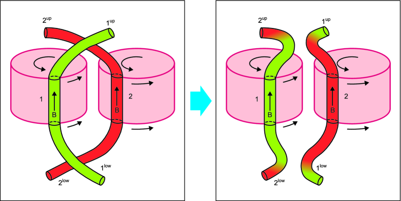
Figure 12: Reconnection diffusion: exchange of flux with entrained matter. Illustration of the mixing of matter and magnetic fields due to reconnection as two flux tubes of different eddies interact. Only one scale of turbulent motions is shown. In real turbulent cascade such interactions proceed at every scale of turbulent motions. From Lazarian11a .

Finally, a number of studies attempted to understand the role of joint action of turbulence and ambipolar diffusion. For instance, Heitschetal04 (henceforth HX04) performed 2.5D simulations of turbulence with two-fluid code and examined the decorrelation of neutrals and magnetic field in the presence of turbulence (see also the Chapter by Zweibel in this volume). The study reported an enhancement of diffusion rate compared to the ambipolar diffusion in a laminar fluid. HX04 correctly associated the enhancement with turbulence creating density gradients that are being dissolved by ambipolar diffusion (see also Zweibel02 ). However, in 2.5D simulations of HX04 the numerical set-up precluded reconnection from taking place as magnetic field was perpendicular to the plane of 2D mixing and therefore magnetic field lines were absolutely parallel to each other. This will not happen in realistic astrophysical situations where reconnection will be an essential part of the physical picture. Therefore, we claim that a treatment of “turbulent ambipolar diffusion” without addressing the reconnection issue is of academic interest.

Incidentally, the authors of HX04 reported an enhanced rate that is equal to the turbulent diffusion rate $LV_{L}$. The fact that ambipolar diffusion rate does not enter the result in HX04 suggests that ambipolar diffusion is irrelevant for the diffusion of matter in the presence of turbulence. This is another reason not to call the observed process “turbulent ambipolar diffusion” .

Therefore we believe that HX04 captured in their simulations a special degenerate case of 2.5D turbulent diffusion where due to a special set up the reconnection is avoided and magnetic field lines do not intersect. We also note that, in the presence of turbulence, the independence of the gravitational collapse from the ambipolar diffusion rate was reported in numerical simulations by Balsaraetal01 , although further higher resolution studies are still missing..

A comprehensive review dealing with reconnection diffusion is presented in Lazarian13 .

7.4 Heat and cosmic ray transport in the presence of reconnection

Magnetic reconnection is a very fundamental basic process that happens in all magnetized fluids. As we discussed in §3 magnetic reconnection is closely related to the turnover processes of magnetic eddies as well as magnetic field wandering. The former is essential for the heat advection via turbulent mixing of magnetized gas. The process was invoked by Choetal03 to explain the suppression of cooling flows in galaxy clusters. Fast LV99 magnetic reconnection was invoked to justify the existence of magnetic eddies for the very high Lundquist number plasmas (see more Lazarian09 ; Lazarian11b ).

Heat transport is also possible in magnetized plasma if electrons are streaming along meandering magnetic field lines. In Lazarian06 the heat transfer by electron streaming was compared with that induced by turbulent eddies and it was concluded that in typical clusters of galaxies the latter dominates.

Transport of cosmic rays along meandering magnetic field was invoked to solve the problem of perpendicular diffusion in Milky Way in classical studies Jokipii73 . For the propagation of cosmic rays the dynamics of turbulent magnetized plasmas is not important as $c/V_{A}$ is usually large. However, the formation of the complicated web of the wandering magnetic field lines that is consistent with the Kolmogorov-type scaling of turbulence statistics does necessarily require fast magnetic reconnection.

7.5 Reconnection and First-order Fermi acceleration

The process of LV99 reconnection invokes shrinking magnetic loops. It is clear from Figure 1 in the Chapter by de Gouveia Dal Pino and Kowal in this volume that particles entrained on such a loop will experience acceleration. This process that naturally follows from the LV99 model was invoked by deGouveiadalPinoLazarian05 to predict efficient First-Order Fermi acceleration of cosmic rays in the reconnection regions (see also Lazarian05 ). The latter are traditionally associated with the acceleration of particles in shocks. Later research revealed the high promise of the process for explaining various physical processes. Recently, the acceleration of cosmic rays in reconnection has been invoked to explain results on the anomalous cosmic rays obtained by Voyager spacecrats (LazarianOpher09 ; Drakeetal10 ), the local anisotropy of cosmic rays (LazarianDesiati10 ) and the acceleration of cosmic rays in clusters of galaxies (LazarianBrunetti11 ), as well as in the surrounds of compact sources and black holes deGouveiadalPinoLazarian05 and relativistic jets Giannios13 . Naturally, the process of acceleration is much more widespread and not limited to the explored examples.

In addition to the acceleration of cosmic rays parallel to magnetic field, acceleration perpendicular to the magnetic field is also possible, as discussed in Kowaletal12b ; Lazarianetal12b . The advantage of such a perpendicular acceleration is that the gain of energy is taking place every Larmor period of the cosmic ray. The efficiency of perpendicular acceleration was observed in simulations of Kowaletal12b , where the simulations of turbulent reconnection were used to study the acceleration of cosmic rays (see more details in de Gouveia Dal Pino and Kowal’s chapter in this volume).

7.6 Dissipation of turbulence in current sheets

MHD turbulence cascade does not depend on the details of microphysics. However, at sufficiently small scales current sheets are formed and those may dissipate a substantial part of the turbulent cascade. As we discussed in §3 within LV99 model small scale reconnection events may happen due to ordinary Ohmic or plasma effects. In particular, the small scale current sheets can be in the collisionless regime. Therefore it is not easy to distinguish the nature of magnetic reconnection by studying the processes of electron and proton heating.

8 Discussion

8.1 Interrelation of LV99 reconnection and modern understanding of MHD turbulence

MHD turbulence has advanced considerably in the last 20 years. It is easy to understand that strong Alfvénic turbulence that induces Richardson diffusion does require fast reconnection. Indeed, eddy type motions that are produced by such turbulence can happen only if the magnetic field of the eddies relaxes on the time scale of eddy turnover. Calculations in LV99 showed that the GS95 theory GoldreichSridhar95 is self-consistent when the small-scale magnetic reconnection between adjacent turbulent eddies happens with the LV99 predicted rate. This result also follows from the Richardson diffusion that we discussed in the chapter.

by a factor . This rate varies from $\sim V_{A}$ for largest eddies in transAlfvénic turbulence to a small fraction of $V_{A}$ for the smallest eddies. Obviously, no mechanism that produces a fixed reconnection rate, e.g. the rate of $0.1V_{A}$ that for decades was a sort of Holy Grail rate for the researchers attempting to explain Solar flares, can make modern theories of MHD turbulence, both the GS95 and its existing modifications, self-consistent. At the same time, ELV11 showed that the Lagrangian dynamics of turbulent fluids do require fast magnetic reconnection. Or, reversing the role of cause and effect, the Lagrangian phenomenon of Richardson dispersion produces a breakdown in the standard form of flux-freezing for a turbulent MHD flow. The reconnection rates that are dictated by the well-established process of Richardson diffusion coincide with those predicted by LV99.

In other words, LV99 reconnection is an intrinsic and inseparable element of MHD turbulence. There can be other types of magnetic reconnection, that are important in particular circumstances, but in turbulent fluids the LV99 type seems inevitable.

8.2 Suggestive evidence on fast reconnection

A study of tearing instability of current sheets in the presence of background 2D turbulence that observed the formation of large-scale islands was performed in Politanoetal89 . While one can argue that observed long-lived islands are the artifact of adopted 2D geometry, the authors present evidence for fast energy dissipation in 2D MHD turbulence and show that this result does not change as they change the resolution. A more recent work of MininniPouquet09 provides evidence for fast dissipation also in 3D MHD turbulence. This phenomenon is consistent with the idea of fast reconnection, but cannot be treated as a direct evidence of the process. Although related, fast dissipation and fast magnetic reconnection are rather different physical processes, dealing with decrease of energy on the one hand and decrease of magnetic flux on the other.

Works by Galsgaard and Nordlund, in particular GalsgaardNordlund97b , could also be interpreted as an indirect support for fast reconnection. The authors showed that in their simulations they could not produce highly twisted magnetic fields. One possible interpretation of this result could be the fast relaxation of magnetic field via reconnection. In this case, these observations could be related to the numerical finding of LapentaBettarini11 which shows that reconnecting magnetic configurations spontaneously get chaotic and dissipate, which, as discussed in LapentaLazarian12 , may be related to the LV99 model. However, in view of many uncertainties of the numerical studies, this relation is unclear. The highest resolution simulations of GalsgaardNordlund97b were only $136^{3}$ and with Reynolds number so small that they could not allow a turbulent inertial-range.

8.3 Convergence of different approaches to fast reconnection

The LV99 model of magnetic reconnection in the presence of weakly stochastic magnetic fields was proposed more than a decade ago. In fact, LV99 and the idea of collisionless X-point reconnection mediated by the Hall effect are essentially coeval. At the same time, due to a few objective factors, it met less enthusiasm in the community than the X-point collisionless reconnection. One can speculate what were the factors responsible for this slow start. For one thing, the collisionless X-point reconnection was initiated and supported by numerical simulations, while the numerical testing of LV99 became possible only recently. In addition, the acceptance of the idea of astrophysical fluids generically being in turbulent state was only taking roots in 1999 (but see Chandrasekhar49 !) and at that time it had much less observational support. By now we have much more evidence which justifies the claim that models ignoring pre-existent turbulence have little relevance to astrophysics. Finally, the analytical solutions of LV99 were based on the use and extension of the GS95 model of turbulence. However, the GS95 theory was far from being universally accepted at the time LV99 was published.

The situation has changed substantially by now. With GS95, as we discussed earlier, being widely accepted, with more observational evidence of ubiquitous turbulence in astrophysical environments and with the successful testing of the LV99 model, it is more difficult to argue against the importance of turbulence for astrophysical reconnection. Moreover, the LV99 model has received more support from solar observations §5, which both showed that magnetic reconnection can be fast in collisional media, where the aforementioned collisionless reconnection does not work. Solar observations also confirmed LV99 predictions on the thickness of reconnection regions and on triggering reconnecttion by the neighboring reconnection events. Last, but not the least, a very important development took place, namely, the LV99 model was connected to the modern developments in the Lagrangian description of magnetized fluids and the equivalence of the approach in LV99 and that based on spontaneous stochasticity was established (see §3 and §4).

One can argue that we have observed the convergence of LV99 with other directions of reconnection research. In particular, recent models of collisionless reconnection have acquired several features in common with the LV99 model. In particular, they have moved to consideration of volume-filling reconnection (see Drakeetal06 ). While much of the discussion may still be centered around 2D magnetic islands produced by reconnection, in three dimensions these islands are expected to evolve into contracting 3D loops or ropes Daughtonetal08 , which is broadly similar to what is depicted in Figure 11, at least in the sense of introducing stochasticity to the reconnection zone. Moreover, it is more and more realized that the 3D geometry of reconnection is essential and that the 2D physics is not adequate and may be misleading. This essentially means the end of the epoch of the dominance of collisionless X-point reconnection. The interest of the models alternative to LV99 shifted to chaotically broadened extended Y-shaped outflow regions, which were advocated in LV99 and confirmed by observations.

The departure from the concept of laminar reconnection and the introduction of magnetic stochasticity is also apparent in a number of recent papers appealing to the tearing mode instability to drive fast reconnection (see Loureiroetal09 , Bhattacharjeeetal09 ). These studies showed that tearing modes do not require collisionless environments and thus collisionality is not a necessary ingredient of fast reconnection. Finally, the reported development of turbulence in 3D numerical simulations clearly testifies that the reconnection induces turbulence even if the initial reconnection conditions are laminar. Naturally, one should expect that turbulence modifies tearing instability and induces its own laws for reconnection thus making for many situations the tearing modes only the trigger to self-supported turbulent reconnection. If this is the case, the final non-linear stage of the reconnection should allow a theoretical description based on the LV99 model.

All in all, in the last decade, the models competing with LV99 have undergone a substantial evolution, from 2D collisionless X-point reconnection based mostly on Hall effect to 3D reconnection where the collisionless condition is no more required, Hall effect is not employed, but magnetic stochasticity and turbulence play an important role in the thick Y-shaped reconnection regions. In other words, a remarkable convergence has taken place.

Saying all the above, we want to stress that collisionless X-point reconnection may nevertheless be suitable for the description of reconnection when the reconnecting flux-structures are comparable with the ion gyro scale, which is the case of the reconnection studied situ in the magnetosphere (see Table LABEL:tab:parameters). However, this is a special case of magnetic reconnection with, we argue, atypical features compared with most astrophysical reconnection.

8.4 Recent attempts to relate turbulence and reconnection

Gue et al. Guoetal12 proposed a model based on the earlier idea of mean field approach suggested initially in KimDiamond01 . In the latter paper the author concluded that the reconnection rate should be always slow in the presence of turbulence. On the contrary, models in Guoetal12 invoke hyperresistivity and get fast reconnection rates. Similarly, invoking the mean field approach HigashimoriHoshino12 presented their model of turbulent reconnection.

The mean field approach invoked in the aforementioned studies was critically analyzed by Eyink11 , and below we briefly present some arguments from that study. The principal difficulty is with the justification of using the mean field approaches to explain fast magnetic reconnection. In such an approach effects of turbulence are described using parameters such as anisotropic turbulent magnetic diffusivity and hyper-resistivity experienced by the fields once averaged over ensembles. The problem is that it is the lines of the full magnetic field that must be rapidly reconnected, not just the lines of the mean field. ELV11 stress that the former implies the latter, but not conversely. No mean-field approach can claim to have explained the observed rapid pace of magnetic reconnection unless it is shown that the reconnection rates obtained in the theory are strictly independent of the length and timescales of the averaging. More detailed discussion of the conceptual problems of the hyper-resistivity concept and mean field approach to magnetic reconnection is presented in Lazarianetal04 and ELV11.

8.5 Reconnection and numerical simulations

As discussed in section §4.1, a brute force numerical approach to astrophysical reconnection is impossible. Therefore our numerical studies of reconnection diffusion in SantosLimaetal10 ; SantosLimaetal12 ; SantosLimaetal13 ; leao13 deal with a different domain of Lundquist numbers and the theoretical justification why for the given problem the Lundquist number regime is not essential. For the case of reconnection diffusion simulations, LV99 theory predicts that the dynamics of reconnection is independent from the Lundquist number and therefore the reconnection in the computer simulations in the presence of turbulence adequately represents the astrophysical process.

The above numerical results explored the consequences of reconnection diffusion. Similarly, as numerical studies of ambipolar diffusion do not “prove” the very concept of ambipolar diffusion, our studies were not intended to “prove” the idea of reconnection diffusion. Our goal was to demonstrate that, in agreement with the theoretical expectations, the process of reconnection diffusion is important for a number of astrophysical set-ups relevant to star formation.

8.6 Plasma physics and reconnection

We have been primarily interested in this review in reconnection phenomena at scales much larger than the ion gyro-radius $\rho_{i}.$ We have also made the claim— which may appear paradoxical to some—that these phenomena can be explained by hydrodynamical processes in turbulent MHD regimes. Microscopic plasma processes do play a role, however, which should be briefly explained. Consider a collisionless turbulent plasma, such as the solar wind, in which the MHD description of the cascade terminates at the ion gyro radius. At scales smaller than $\rho_{i}$ but larger than $\rho_{e}$, the plasma is described by an ion kinetic equation and a system of “electron reduced MHD” (ERMHD) equations for kinetic Alfvén waves Schekochihinetal07 ; Schekochihinetal09 . This system exhibits the “Hall effect”, with distinct ion and electron mean flow velocities and magnetic field-lines frozen-in to the electron fluid. The ERMHD equations (or the more general “electron MHD” or EMHD equations) produce the typical features of “Hall reconnection” such as quadrupolar magnetic fields in the reconnection zone UzdenskyKuslrud06 . At length scales smaller than $\rho_{e},$ kinetic equations are required to describe both the ions and the electrons. It is at these scales that the magnetic flux finally “unfreezes” from the electron fluid, due to effects such as Ohmic resistivity, electron inertia, finite electron gyroradius, etc. However, as we have discussed at length in this review, these weak effects are vastly accelerated by turbulent advection and manifested, in surprising ways, at far larger length scales.

- (1) Alfvén, H. 1942, Ark. Mat., Astron. o. Fys., 29B, 1
- (2) Parker, E. N. 1979, Oxford, Clarendon Press; New York, Oxford University Press, 1979, 858 p.,
- (3) Parker, E. N. 1970, The Astrophysical Journal, 162, 665
- (4) Lovelace, R. V. E. 1976, Nature, 262, 649
- (5) Priest, E. R., & Forbes, T. G. 2002, Astronomy & Astrophysics Reviews, 10, 313
- (6) Innes, D. E., Inhester, B., Axford, W. I., & Wilhelm, K. 1997, Nature, 386, 811
- (7) Yokoyama, T., & Shibata, K. 1995, Nature, 375, 42
- (8) Masuda, S., Kosugi, T., Hara, H., Tsuneta, S. & Ogawara, Y. 1994, Nature, 371, 495
- (9) Shay, M. A., Drake, J. F., Denton, R. E., & Biskamp, D. 1998, Journal of Geophysical Research, 103, 9165
- (10) Drake, J. F. 2001, Nature, 410, 525
- (11) Drake, J. F., Swisdak, M., Che, H., & Shay, M. A. 2006, Nature, 443, 553
- (12) Daughton, W., Scudder, J., & Karimabadi, H. 2006, Physics of Plasmas, 13, 072101
- (13) Parker, E. N. 1993, The Astrophysical Journal, 408, 707
- (14) Ossendrijver, M. 2003, Astronomy & Astrophysics Reviews, 11, 287
- (15) Sturrock, P. A. 1966, Nature, 211, 695
- (16) Zhang, B., & Yan, H. 2011, The Astrophysical Journal, 726, 90
- (17) Lazarian, A., Vishniac, E. T., & Cho, J. 2004, The Astrophysical Journal, 603, 180
- (18) Fox, D. B., et al. 2005, Nature, 437, 845
- (19) Galama, T. J., et al. 1998, Nature, 395, 670
- (20) Shibata, K. & Magara, T. 2001, Living Reviews in Solar Physics, 8, 6
- (21) Browning, P., & Lazarian, A., 2013, Space Science Reviews, 178, 325
- (22) Karimabadi, H. & Lazarian, A. 2013, Physics of Plasmas, in press
- (23) Kowal, G., Lazarian, A., Vishniac, E. T., & Otmianowska-Mazur, K. 2009, The Astrophysical Journal, 700, 63
- (24) Parker, E. N. 1957, Journal of Geophysical Research, 62, 509
- (25) Sweet, P. A. 1958, Proceedings from IAU Symposium no. 6. edited by Bo Lehnert, Cambridge University Press, p. 123
- (26) Petschek, H. E. 1964, The Physics of Solar Flares, AAS-NASA Symposium (NASA SP-50), ed. W. H. Hess (Greenbelt, MD: NASA), 425
- (27) Biskamp, D. 1996, Astrophysics and Space Science, 242, 165
- (28) Shay, M. A., Drake, J. F., & Swisdak, M. M. 2004, Physics of Plasmas, 11, 2199
- (29) Bhattacharjee, A., Ma, Z. W., & Wang, X. 2003, Lecture Notes in Physics, 614, 351
- (30) Wang, X., Bhattacharjee, A., & Ma, Z. W. 2001, Physical Review Letters, 87, 265003
- (31) Smith, D., Ghosh, S., Dmitruk, P., & Matthaeus, W. H. 2004, Geophysysical Research Letters, 31, L02805
- (32) Fitzpatrick, R. 2004, Physics of Plasmas, 11, 937
- (33) Malyshkin, L. M. 2008, Physical Review Letters, 101, 225001
- (34) B. K. Shivamoggi, 2011, Phys. Plasmas 18, 052304
- (35) Yamada, M. 2007, Physics of Plasmas, 14, 058102
- (36) Norman, C. A., & Ferrara, A. 1996, The Astrophysical Journal, 467, 280
- (37) Ferrière, K. M. 2001, Reviews of Modern Physics, 73, 1031
- (38) Subramanian, K., Shukurov, A., & Haugen, N. E. L. 2006, Monthly Notices of Royal Astronomical Society, 366, 1437
- (39) Enßlin, T. A., & Vogt, C. 2006, Astronomy & Astrophysics, 453, 44
- (40) Chandran, B. D. G. 2005, The Astrophysical Journal, 632, 809
- (41) Balbus, S. A., & Hawley, J. F. 1998, Reviews of Modern Physics, 70, 1
- (42) Galsgaard, K., & Nordlund, Å. 1997, Journal of Geophysical Research, 102, 219
- (43) Gerrard, C. L., & Hood, A. W. 2003, Solar Physics, 214, 151
- (44) Leamon, R. J., Smith, C. W., Ness, N. F., Matthaeus, W. H., & Wong, H. K. 1998, Journal of Geophysical Research, 103, 4775
- (45) Bale, S. D., Kellogg, P. J., Mozer, F. S., Horbury, T. S., & Reme, H. 2005, Physical Review Letters, 94, 215002
- (46) Schuecker, P., Finoguenov, A., Miniati, F., Böhringer, H., & Briel, U. G. 2004, Astronomy & Astrophysics, 426, 387
- (47) Vogt, C., & Enßlin, T. A. 2005, Astronomy & Astrophysics, 434, 67
- (48) Armstrong, J. W., Rickett, B. J., & Spangler, S. R. 1995, The Astrophysical Journal, 443, 209
- (49) Chepurnov, A. & Lazarian, A. 2010, The Astrophysical Journal, 710, 853
- (50) Eyink, G. L. 2008, Physica D Nonlinear Phenomena, 237, 1956
- (51) Lazarian, A. & Pogosyan, D. 2000, The Astrophysical Journal, 537, 720
- (52) Lazarian, A. & Pogosyan, D. 2004, The Astrophysical Journal, 616, 943
- (53) Lazarian, A. & Pogosyan, D. 2006, The Astrophysical Journal, 652, 1348
- (54) Lazarian, A. & Pogosyan, D. 2008, The Astrophysical Journal, 686, 350
- (55) Lazarian, A. 2009, Space Science Reviews, 143, 357
- (56) Vekshtein, G. E., Ryutov, D. D., & Sagdeev, R. Z. 1970, Soviet Journal of Experimental and Theoretical Physics Letters, 12, 291
- (57) Kulsrud, R. 1983, Handbook of Plasma Physics, eds. M. N. Rosenbluth & R. Z. Sagdeev (North Holland, New York)
- (58) Eyink, G. L., Lazarian, A., & Vishniac, E. T. 2011, The Astrophysical Journal, 743, 51
- (59) Braginsky, S. I. 1965. Rev. Plasma Phys. 1, 205.
- (60) Fitzpatrick, R. 2011, “Introduction to Plasma Physics”, online lecture notes, URL: http://farside.ph.utexas.edu/teaching/plasma/plasma.html
- (61) Bemporad, A. 2008, The Astrophysical Journal, 689, 572
- (62) Zimbardo, G., Greco, A., Sorriso-Valvo, L., Perri, S., Vörös, Z., Aburjania, G., Chargazia, K., & Alexandrova, O. 2010, Space Science Reviews, 156, 89
- (63) Kowal, G., Falceta-Gonçalves, D. A., & Lazarian, A. 2011, New Journal of Physics, 13, 053001
- (64) Santos-Lima, R., de Gouveia Dal Pino, E. M., Kowal, G., Falceta-Gonçalves, D. A., Lazarian, A., & Nakwacki, M. S. 2013, The Astrophysical Journal, in press, arXiv:1305.5654
- (65) Schekochihin, A. A., Cowley, S. C., Maron, J. L., & McWilliams, J. C. 2004, The Astrophysical Journal, 612, 276
- (66) Schekochihin, A. A., & Cowley, S. C. 2006, Physics of Plasmas, 13, 056501
- (67) Lazarian, A., & Beresnyak, A. 2006, Monthly Notices of the Royal Astronomical Society, 373, 1195
- (68) Schekochihin, A. A., Cowley, S. C., & Dorland, W. 2007, Plasma Physics and Controlled Fusion, 49, 195
- (69) Schekochihin, A. A., Cowley, S. C., Dorland, W., Hammett, G. W., Howes, G. G., Quataert, E., & Tatsuno, T. 2009, The Astrophysical Journals, 182, 310
- (70) Cho, J., & Lazarian, A. 2002, Physical Review Letters, 88, 245001
- (71) Cho, J., & Lazarian, A. 2003, Monthly Notices of Royal Astronomical Society, 345, 325
- (72) Kowal, G., & Lazarian, A. 2010, The Astrophysical Journal, 720, 742
- (73) Goldreich, P. & Sridhar, S. 1995, The Astrophysical Journal, 438, 763
- (74) Lithwick, Y., & Goldreich, P. 2001, The Astrophysical Journal, 562, 279
- (75) Biskamp, D. 2003, Magnetohydrodynamic Turbulence, by Dieter Biskamp, pp. 310. ISBN 0521810116. Cambridge, UK: Cambridge University Press, September 2003.,
- (76) Shebalin, J. V., Matthaeus, W. H., & Montgomery, D. 1983, Journal of Plasma Physics, 29, 525
- (77) Higdon, J. C. 1984, The Astrophysical Journal, 285, 109
- (78) Lazarian, A. & Vishniac, E. T. 1999, The Astrophysical Journal, 517, 700
- (79) Cho, J., & Vishniac, E. T. 2000, The Astrophysical Journal, 539, 273
- (80) Maron, J., & Goldreich, P. 2001, The Astrophysical Journal, 554, 1175
- (81) Cho, J., Lazarian, A., & Vishniac, E. T. 2002, The Astrophysical Journal, 564, 291
- (82) Podesta, J. J. 2010, Twelfth International Solar Wind Conference, 1216, 128
- (83) Wicks, R. T., Horbury, T. S., Chen, C. H. K. & Schekochihin, A. A. 2010, Monthly Notices of Royal Astronomical Society, 407, L31
- (84) Wicks, R. T., Horbury, T. S., Chen, C. H. K. & Schekochihin, A. A. 2011, Physical Review Letters, 106, 045001
- (85) Montgomery, D. & Matthaeus, W. H. 1995, The Astrophysical Journal, 447, 706
- (86) Galtier, S., Nazarenko, S. V., Newell, A. C. & Pouquet, A. 2000, J. Plasma Phys., 63, 447
- (87) Ng, C. S. & Bhattacharjee, A. 1996, The Astrophysical Journal, 465, 845
- (88) Lazarian, A. 2006, The Astrophysical Journal Letters, 645, L25
- (89) Cho, J., Lazarian, A., & Vishniac, E. T. 2003, Turbulence and Magnetic Fields in Astrophysics, 614, 56
- (90) Boldyrev, S. 2006, Phys. Rev. Lett., 96, 115002
- (91) Beresnyak, A., & Lazarian, A. 2006, The Astrophysical Journal Letters, 640, L175
- (92) Beresnyak, A., & Lazarian, A. 2009, The Astrophysical Journal, 702, 1190
- (93) Gogoberidze, G. 2007, Physics of Plasmas, 14, 022304
- (94) Beresnyak, A., & Lazarian, A. 2010, The Astrophysical Journal Letters, 722, L110
- (95) Beresnyak, A. 2011, Physical Review Letters, 106, 075001
- (96) Beresnyak, A. 2012, Monthly Notices of the Royal Astronomical Society, 422, 3495
- (97) Brandenburg, A. & Lazarian, A., 2013, Space Science Reviews, in press
- (98) Ya B Zeldovich, 1957, JETP Phys 4, 460
- (99) Speiser, T. W. 1970, Planetary Space Science, 18, 613
- (100) Jacobson, A. R., & Moses, R. W. 1984, Physical Review A, 29, 3335
- (101) Strauss, H. R. 1986, Physics of Fluids, 29, 3668
- (102) Bhattacharjee, A., & Hameiri, E. 1986, Physical Review Letters, 57, 206
- (103) Hameiri, E., & Bhattacharjee, A. 1987, Physics of Fluids, 30, 1743
- (104) Diamond, P. H., & Malkov, M. 2003, Physics of Plasmas, 10, 2322
- (105) Strauss, H. R. 1988, The Astrophysical Journal, 326, 412
- (106) Shibata, K. & Tanuma, S. 2001, Earth Planets Space, 53, 473
- (107) Waelbroeck, F. L. 1989, Physics of Fluids B, 1, 2372
- (108) Loureiro, N. F., Uzdensky, D. A. , Schekochihin, A. A., Cowley, S. C. & Yousef, T. A. 2009, Mon. Not. R. Astron. Soc., 399, L146
- (109) Bhattacharjee, A., Huang, Y.-M., Yang, H. & Rogers, B. 2009, Phys. Plasmas, 16, 112102
- (110) Karimabadi, H., Roytershteyn, V., Wan, M., et al. 2013, Physics of Plasmas, 20, 012303
- (111) Beresnyak, A. 2013, arXiv:1301.7424
- (112) Dahlburg, R. B., Antiochos, S. K., & Zang, T. A. 1992, Physics of Fluids B, 4, 3902
- (113) Dahlburg, R. B., & Karpen, J. T. 1994, Space Science Reviews, 70, 93
- (114) Dahlburg, R. B. 1997, Journal of Plasma Physics, 57, 35
- (115) Ferraro, N. M., & Rogers, B. N. 2004, Physics of Plasmas, 11, 4382
- (116) Matthaeus, W. H. & Lamkin, S. L. 1985, Physics of Fluids, 28, 303
- (117) Matthaeus, W. H. & Lamkin, S. L. 1986, Physics of Fluids, 29, 2513
- (118) Watson, P. G., Oughton, S. & Craig, I. J. D. 2007, Physic. Plasmas, 14, 032301
- (119) Eyink, G. L., & Benveniste, D. 2013, Phys. Rev. E, 88, 041001
- (120) Kupiainen, A. 2003, Ann. Henri Poincaré, 4, Suppl. 2, S713
- (121) Yamada, M., Ren, Y., Ji, H., Breslau, J., Gerhardt, S., Kulsrud, R., & Kuritsyn, A. 2006, Physics of Plasmas, 13, 052119
- (122) Kowal, G., Lazarian, A., Vishniac, E. T., & Otmianowska-Mazur, K. 2012, Nonlinear Processes in Geophysics, 19, 297
- (123) Vishniac, E. T., Pillsworth, S., Eyink, G. L., Kowal, G., Lazarian, A., Murray, S. 2012, Nonlinear Processes in Geophysics, 19, 605
- (124) Maron, J., Chandran, B. D., & Blackman, E. 2004, Physical Review Letters, 92, 045001
- (125) Beresnyak, A. 2013, The Astrophysical Journal Letters, 767, L39
- (126) Eyink, G. L., Vishniac, E. T., Lalescu, C., Aluie, H., Kanov, K., Bürger, K., Burns, R., Meneveau, C. and Szalay, A. 2013. Nature, 497, 466
- (127) Ciaravella, A., & Raymond, J. C. 2008, The Astrophysical Journal, 686, 1372
- (128) Drake, J. F., Opher, M., Swisdak, M., & Chamoun, J. N. 2010, The Astrophysical Journal, 709, 963
- (129) Sych, R., Nakariakov, V. M., Karlicky, M., & Anfinogentov, S. 2009, Astronomy & Astrophysics, 505, 791
- (130) Gosling, J. T., 2012, Space Science Reviews, 172, 187
- (131) J. T. Gosling,T. D. Phan, R. P. Lin, and A. Szabo 2007, Geophys. Res. Lett. 34, L15110
- (132) J. T. Gosling and A. Szabo 2008, J. Geophys. Res. 113, A10103
- (133) B. J. Vasquez, V. I. Abramenko, D. K. Haggerty, and C. W. Smith 2007, J. Geophys. Res. 112, A11102
- (134) T. D. Phan, J. T. Gosling, and M. S. Davis 2009, Geophys. Res. Lett. 36, L09108
- (135) Lazarian, A. and Opher, M. 2009, The Astrophysical Journal, 703, 8
- (136) S.-Y. Huang et al. 2012, Geophys. Res. Lett., 39, L11104
- (137) Rechester, A. B., & Rosenbluth, M. N. 1978, Physical Review Letters, 40, 38
- (138) Vishniac, E. & Lazarian, A. 1999, in: Plasma Turbulence and Energetic Particles in Astrophysics; Proceedings of the International Conference, Cracow, Poland, 5-10 September, 1999 eds. M. Ostrowski & R. Schlickeiser. Obserwatorium Astronomiczne, Uniwersytet Jagielloński, Kraków.
- (139) Heitsch, F., & Zweibel, E. G. 2003, The Astrophysical Journal, 583, 229
- (140) Leake, J. E., Lukin, V. S., Linton, M. G., & Meier, E. T. 2012, The Astrophysical Journal, 760, 109
- (141) Lazarian, A., & Vishniac, E. T. 2009, Revista Mexicana de Astronomia y Astrofisica Conference Series, 36, 81
- (142) Kowal, G., Lazarian, A., Falceta-Gonçalves, D. A., & Vishniac, E. T., in preparation
- (143) R. Susino, A. Bemporad, and S. Kruker, arXiv:1310.2853v1 [astro-ph.SR]
- (144) Kraichnan, R. H. 1965, Phys. Fluids, 8, 1385
- (145) Kim, E.-j., & Diamond, P. H. 2001, The Astrophysical Journal, 556, 1052
- (146) Cho, J., 2005, The Astrophysical Journal, 621, 324
- (147) Cho, J. & Lazarian, A. 2013, The Astrophysical Journal Letters, in press
- (148) Lazarian, A., Petrosian, V., Yan, H., & Cho, J. 2003, arXiv:astro-ph/0301181
- (149) Kulsrud, R. 2005 Princeton University Press, Princeton, NJ
- (150) Bernard, D., Gawȩdzki, K. & Kupiainen, A. 1998, J. Stat. Phys., 90, 519
- (151) Gawȩdzki, K. & Vergassola, M. 2000, Physica D, 138, 63
- (152) E, W. & vanden-Eijnden, E. 2001, Physica D, 152-153, 636
- (153) E, W., & Vanden-Eijnden, E. 2000a, Physics of Fluids, 12, 149
- (154) E, W. & Vanden-Eijnden, E. 2000b, Proceedings of National Academy of Sciences of the United States of America, 97, 8200
- (155) E, W. & Vanden-Eijnden, E. 2001, Physica D: Nonlinear Phenomena, 152, 636
- (156) Chaves, M., Gawȩdzki, K., Horvai, P., Kupiainen, A. & Vergassola, M. 2003, J. Stat. Phys., 113, 643
- (157) Gawȩdzki, K. 2008, arXiv:0806.1949
- (158) S. Chandrasekhar, 1961, Hydrodynamic and Hydromagnetic Stability, Oxford University Press
- (159) M. E. Mandt, R. E. Denton, and J. F. Drake, 1994, Geophys. Res. Lett. 21, 73 (1994)
- (160) Shay, M. A., & Drake, J. F. 1998, Geophysical Review Letters, 25, 3759
- (161) M. Bauer & D. Bernard 1999, J. Phys. A: Math. Gen., 32, 5179
- (162) Eyink, G. L. 2011, Physical Review E, 83, 056405
- (163) Lapenta, G. 2008, Phys. Rev. Lett., 100, 235001
- (164) Beresnyak, A., & Lazarian, A. 2008, The Astrophysical Journal, 682, 1070
- (165) B. J. Lynch et al, 2008, Astrophys. J. 683: 1192
- (166) Giannios, D. 2013, Monthly Notices of the Royal Astronomical Society, 431, 355
- (167) Lazarian, A. 2005, Magnetic Fields in the Universe: From Laboratory and Stars to Primordial Structures., 784, 42
- (168) Santos-Lima, R., Lazarian, A., de Gouveia Dal Pino, E. M., & Cho, J. 2010, The Astrophysical Journal, 714, 442
- (169) Santos-Lima, R., de Gouveia Dal Pino, E. M., & Lazarian, A. 2012, The Astrophysical Journal, 747, 21
- (170) Lazarian, A. 2011a, arXiv:1108.2280
- (171) Lazarian, A., Esquivel, A., & Crutcher, R. 2012, The Astrophysical Journal, 757, 154
- (172) Heitsch, F., Zweibel, E. G., Slyz, A. D., & Devriendt, J. E. G. 2004, The Astrophysical Journal, 603, 165
- (173) Zweibel, E. G. 2002, The Astrophysical Journal, 567, 962
- (174) Balsara, D. S., Crutcher, R. M., & Pouquet, A. 2001, The Astrophysical Journal, 557, 451
- (175) Lazarian, 2013, Space Science Reviews, accepted
- (176) Lazarian, A. 2011b, arXiv:1111.0694
- (177) Jokipii, J. R. 1973, The Astrophysical Journal, 183, 1029.
- (178) de Gouveia dal Pino, E. M., & Lazarian, A. 2005, Astronomy & Astrophysics, 441, 845
- (179) Lazarian, A., & Desiati, P. 2010, The Astrophysical Journal, 722, 188
- (180) Lazarian, A., & Brunetti, G. 2011, Memorie della Societa Astronomica Italiana, 82, 636
- (181) Lazarian, A., Kowal, G., Vishniac, E., & de Gouveia Dal Pino, E. 2011, Planetary and Space Science, 59, 537
- (182) Lazarian, A., Vlahos, L., Kowal, G., Yan, H., Beresnyak, A., de Gouveia Dal Pino, E. M. 2012, Space Science Reviews, 173, 557
- (183) Kowal, G., de Gouveia Dal Pino, E. M., & Lazarian, A. 2012, Physical Review Letters, 108, 241102
- (184) Politano, H., Pouquet, A. & Sulem, P. L. 1989, Physics of Fluids B, 1, 2330
- (185) de Gouveia Dal Pino, E. M., Leão, M. R. M., Santos-Lima, R., Guerrero, G., & Lazarian, A. 2012, Phys. Scripta, 86, 018401
- (186) Leão, M. R. M., de Gouveia Dal Pino, E. M., Santos-Lima, R. & Lazarian, A. 2013, The Astrophysical Journal, 777, 46L
- (187) Mininni, P. D. & Pouquet, A. 2009, Physical Review E, 80, 025401
- (188) Galsgaard, K. & Nordlund, Å. 1997, Journal of Geophysical Research, 102, 231
- (189) Lapenta, G., & Bettarini, L. 2011, arXiv:1102.4791
- (190) Lapenta, G., & Lazarian, A. 2012, Nonlinear Processes in Geophysics, 19, 251
- (191) S. Chandrasekhar, 1949, Astrophys. J. 110, 329
- (192) Daughton, W., Roytershteyn, V., Albright, B. J., Bowers, K., Yin, L., & Karimabadi, H. 2008, AGU Fall Meeting Abstracts, A1705
- (193) Y.-M. Huang et al., 2011, Phys. Plasmas 18, 072109
- (194) Guo, Z. B., Diamond, P. H., & Wang, X. G., 2012, The Astrophysical Journal, 757, 173
- (195) Higashimori, K., & Hoshino, M., 2012, Journal of Geophysical Research (Space Physics), 117, 1220
- (196) Uzdensky, D. A. & Kulsrud, R. M. 2006, Physics of Plasmas, 13, 062305
- (197) Shay, M. A., Drake, J. F., Rogers, B. N., & Denton, R. E. 1999, Geophysical Review Letters, 26, 2163
- (198) Wang, X., Bhattacharjee, A., & Ma, Z. W. 2000, Journal of Geophysical Research, 105, 27 633
- (199) Birn, J., et al. 2001, Journal of Geophysical Research, 106, 3715
- (200) Malakit, K., Cassak, P. A., Shay, M. A., & Drake, J. F. 2009, Geophysical Review Letters, 36, 7107
- (201) Cassak, P. A., Shay, M. A., & Drake, J. F. 2010, Physics of Plasmas, 17, 062105
- (202) Yamada, M. 1999, Journal of Geophysical Research, 104, 14529
- (203) Yamada, M., Kulsrud, R., & Ji, H. 2010, Reviews of Modern Physics, 82, 603