Properties of the Homogeneous Cooling State of a Gas of Inelastic Rough Particles

Abstract

In this work we address the question of whether a low-density system composed of identical rough particles may reach hydrodynamic states (also called normal states), even if energy is not conserved in particle collisions. As a way to measure the ability of the system to present a hydrodynamic behavior, we focus on the so-called homogeneous cooling state of the granular gas and look at the corresponding relaxation time as a function of inelasticity and roughness. We report computer simulation results of the sixth- and eighth-order cumulants of the particle velocity distribution function and study the influence of roughness on their relaxation times and asymptotic values. This extends the results of a previous work [Phys. Rev. E 89, 020202(R) (2014], where lower-order cumulants were measured. Our results confirm that the relaxation times are not necessarily longer for stronger inelasticities. This implies that inelasticity by itself does not preclude hydrodynamics. It is also observed that the cumulants associated with the angular velocity distribution may reach very high values in a certain region of (small) roughness and that these maxima coincide with small orientational correlation points.

1 Introduction

Matter is inherently a many-body system. Logically, for a system with a very large number of particles the accurate description of each entity’s dynamics becomes irrelevant, whereas a statistical picture of the system can yield a meaningful account of the underlying physics Pauli (2000). In matter systems where particles are atoms or molecules, and if the internal dynamics is not relevant in the process of dynamical exchange between particles (henceforth, collisions), we may have two separated dynamics levels: a quantum one for atom dynamics description and a classical one for particle dynamics exchange description Pauli (2000). Therefore, under certain conditions, a classical statistical-mechanical theory is appropriate for the physics resulting from particles collisions. In this case, and for low-density fluids, the classical Boltzmann equation applies Chapman and Cowling (1970).

Furthermore, the statistical description resulting from the Boltzmann equation is amenable to a higher level description called hydrodynamics Batchelor (1953, 1967); Chaikin and Lubensky (2000). In the hydrodynamic approach, low density states are characterized by a single particle distribution function (“normal” solution) whose spatial dependence may be written entirely through a functional dependence on the relevant average fields. These fields appear in the appropriate balance equations of the system Chaikin and Lubensky (2000); Goldhirsch (2003). The three basic fields are density, flow velocity, and temperature, resulting from mass, momentum, and energy balance, respectively.

Let us now suppose that our system has indeed a large number of particles at low density but that these are not atoms or molecules but much larger particles (typical size of at least $1~{}\mu$m), that we can call grains Bagnold (1954). Would then the hydrodynamic description work at a theoretical level? Would the behavior of this kind of systems look like that of a classical fluid? Dufty and Brey (2011) Obviously, “fluid” properties are present in some peculiar way. In fact, many phenomena present in classical fluids, such as instabilities, convection, diffusion, thermal segregation, laminar flow, etc., are analogously present in low-density granular systems Goldhirsch (2003); Jaeger et al. (1996). Thus, at a theoretical and fundamental level an important question arises: are the equations of fluid mechanics appropriate for a many-particle system at low density, independently of the size of its particles, even if collisions dissipate energy? At a “real life” level the answer to this question is important and far reaching since a positive answer would imply that we can find fluid-like behavior (and apply the appropriate tools) in a wealth of very common systems (sands, asteroid rings, powders, stone avalanches, cereal mills, etc.) Jaeger et al. (1996).

The aim of this work is to support the growing evidence that, indeed, fluid mechanics should in principle be appropriate for low-density granular systems without a priori limitation on the degree of inelasticity in particle collisions Dufty and Brey (2011), even if particle roughness is significant. Our results will also allow us to show that, on the other hand, the distribution function of the granular gas of rough spheres may strongly deviate from the Maxwellian.

In this work, we consider a system with a large number of identical particles that may eventually collide loosing a fraction of their kinetic energy. The system is at very low density and thus collisions are always binary and instantaneous. Therefore, our system is a granular gas that may be described by the inelastic versions of the Boltzmann and/or Enskog equations Brilliantov and Pöschel (2004); Garzó et al. (2007); Vega Reyes et al. (2010, 2014). We let our particle velocities have translational and rotational degrees of freedom. For simplicity, we will assume that the momentum transfer in collisions occurs with no sliding between the particles. Therefore, collisions may be characterized by the coefficients of normal and tangential restitution Brilliantov et al. (2007), measuring the degrees of inelasticity and roughness, respectively. We also assume that those coefficients are constant (i.e., they do not depend on the velocities of the colliding particles).

For this rough hard-sphere model, we show by computer simulations that, after a transient, the undriven system relaxes always to a “normal” (or hydrodynamic) state, the so-called homogeneous cooling state (HCS), the relaxation stage length being practically not related to the degree of inelasticity (coefficient of normal restitution) in the collisions. Furthermore, in the range of interest for experiments (medium or large roughness), this relaxation time does not present a clear tendency with respect to the degree of roughness of the particles (coefficient of tangential restitution) either. However, the system seems to have very long relaxation times near the smooth collision limit (i.e., at small particle roughness). Moreover, strong non-Maxwellian effects are present within a certain range of roughness. These findings are based on measurements of sixth- and eighth-order velocity cumulants, thus complementing a previous study based on the fourth-order cumulants Vega Reyes et al. (2014).

2 The inelastic rough hard-sphere model

We consider in a volume $V$ a set of $N=nV$ identical hard spheres with diameter $\sigma$, mass $m$, and moment of inertia $I$. Each sphere possesses a translational and an angular velocity $\mathbf{v}$ and $\bm{\omega}$, respectively, and collisions are binary and instantaneous. In addition, the spheres are dissipative, i.e., a fraction of kinetic energy is lost during collisions.

The collisional model we will use is the inelastic rough hard-sphere model Chapman and Cowling (1970); Brilliantov et al. (2007); Goldhirsch et al. (2005), in which collisions are characterized by two (constant) coefficients of restitution: $\alpha$ for normal restitution and $\beta$ for tangential restitution Vega Reyes et al. (2014):

$$\widehat{\bm{\sigma}}\cdot\mathbf{v}^{\prime}_{12}=-\alpha\widehat{\bm{\sigma}}\cdot\mathbf{v}_{12},\quad\widehat{\bm{\sigma}}\times\mathbf{v}^{\prime}_{12}=-\beta\widehat{\bm{\sigma}}\times\mathbf{v}_{12},$$ (1)

where $\widehat{\boldsymbol{\sigma}}$ is a unit vector directed along the centers of the two colliding particles, $\mathbf{v}_{12}$ is the relative velocity of the contact points of the colliding pair of particles, and primes denote post-collisional values. The coefficient of normal restitution ranges from $\alpha=0$ (completely inelastic collision) to $\alpha=1$ (perfectly elastic collision), while the coefficient of tangential restitution (or “roughness” parameter) ranges from $\beta=-1$ (perfectly smooth particles, with no reversal of tangential relative velocity) to $\beta=1$ (perfectly rough particles, with perfect reversal of tangential relative velocity). For a complete description of the collisional rules, we refer the reader to Refs. Brilliantov et al. (2007); Santos et al. (2011).

Under spatially homogeneous conditions, the Enskog kinetic equation in its inelastic version applies,

$$\frac{\partial f}{\partial t}={\chi(n)J}[\mathbf{v},\bm{\omega}|f],$$ (2)

where $f(\mathbf{v},\bm{\omega},t)$ is the one-body velocity distribution function, $\chi(n)$ is the pair correlation function at contact (Enskog factor) Hansen and McDonald (2006), and $J$ is the Boltzmann collision operator for inelastic rough hard spheres (for an explicit expression of this operator, see Ref. Santos et al. (2011)). Given a certain dynamical variable $A(\mathbf{v},\bm{\omega})$, its average value is given by

$${\langle A\rangle=\frac{1}{n}\int d\mathbf{v}\int d\bm{\omega}\,A(\mathbf{v},\bm{\omega})f(\mathbf{v},\bm{\omega},t)}.$$ (3)

As usual Brilliantov et al. (2007); Santos et al. (2011), the translational and rotational temperatures are defined as

$${T_{t}=\frac{m}{3}\langle(\mathbf{v}-\mathbf{u}_{f})^{2}\rangle,\quad T_{r}=\frac{I}{3}\langle\omega^{2}\rangle,}$$ (4)

respectively, where $\mathbf{u}_{f}=\langle\mathbf{v}\rangle$ is the flow velocity. Due to energy dissipation, the total temperature $T=\frac{1}{2}(T_{t}+T_{r})$ decays monotonically with time (unless $\alpha=\beta^{2}=1$). Since for the kinetic equation (2) both the density $n$ and $\mathbf{u}_{f}$ are constant, $T$ is the only relevant hydrodynamic quantity of the system. Thus, if a hydrodynamic regime does exist, the whole temporal dependence of $f$ must occur through a dependence on $T$ van Noije and Ernst (1998).

It is then convenient to rescale the translational and angular velocities with the respective temperatures and define the reduced quantities

$${\mathbf{c}(t)\equiv\frac{\mathbf{v}-\mathbf{u}_{f}}{\sqrt{2T_{t}(t)/m}}},\quad{\mathbf{w}(t)\equiv\frac{\bm{\omega}}{\sqrt{2T_{r}(t)/I}}}.$$ (5)

Consequently, the reduced distribution function is

$${\phi(\mathbf{c},\mathbf{w},t)\equiv\frac{1}{n}\left[\frac{4T_{t}(t)T_{r}(t)}{mI}\right]^{3/2}f(\mathbf{v},\bm{\omega},t)}.$$ (6)

In this undriven and spatially homogeneous situation, the existence of a hydrodynamic state (the HCS) implies that, at given $\alpha$ and $\beta$, both the temperature ratio $\theta(t)\equiv T_{r}(t)/T_{t}(t)$ and the reduced distribution function $\phi(\mathbf{c},\mathbf{w},t)$ reach well defined stationary values after a certain relaxation time. This expectation was recently confirmed Vega Reyes et al. (2014) at the level of $\theta(t)$ and of the fourth-order velocity cumulants by computer simulations and a Grad approximation. As said in the Introduction, our main aim here is to extend the simulation test to sixth- and eighth-order cumulants, checking whether the relaxation times are sensitive or not to the order of the cumulants.

3 Velocity cumulants

Now we assume that the state is isotropic. This means that $\phi(\mathbf{c},\mathbf{w},t)$ must be a function of the three scalar quantities $c^{2}=\mathbf{c}\cdot\mathbf{c}$, $w^{2}=\mathbf{w}\cdot\mathbf{w}$, and $(\mathbf{c}\cdot\mathbf{w})^{2}$, so we can represent it as a polynomial expansion of the form Vega Reyes et al. (2014); Santos and Kremer (2012)

$$\phi(\mathbf{c},\mathbf{w},t)={\frac{e^{-c^{2}-w^{2}}}{\pi^{3}}}\sum_{j=0}^{\infty}\sum_{k=0}^{\infty}\sum_{\ell=0}^{\infty}a_{jk}^{(\ell)}(t)\Psi_{jk}^{(\ell)}(\mathbf{c},\mathbf{w}),$$ (7)

where

$$\Psi_{jk}^{(\ell)}(\mathbf{c},\mathbf{w})=L_{j}^{(2\ell+\frac{1}{2})}(c^{2})L_{k}^{(2\ell+\frac{1}{2})}(w^{2})\left(c^{2}w^{2}\right)^{\ell}P_{2\ell}(u)$$ (8)

is a polynomial of total degree $2(j+k+2\ell)$ in velocity. Here, $L_{j}^{(\alpha)}(x)$ and $P_{2\ell}(x)$ are Laguerre and Legendre polynomials, respectively, and $u\equiv(\mathbf{c}\cdot\mathbf{w})/cw$. The set of polynomials $\{\Psi_{jk}^{(\ell)}\}$ constitute a complete orthogonal basis Vega Reyes et al. (2014), i.e.,

$${\langle\Psi_{jk}^{(\ell)}|\Psi_{j^{\prime}k^{\prime}}^{(\ell^{\prime})}\rangle=N_{jk}^{(\ell)}\delta_{j,j^{\prime}}\delta_{k,k^{\prime}}\delta_{\ell,\ell^{\prime}}},$$ (9)

where the normalization constants are

$${N_{jk}^{(\ell)}=\frac{\Gamma(j+2\ell+\frac{3}{2})\Gamma(k+2\ell+\frac{3}{2})}{[\Gamma(\frac{3}{2})]^{2}(4\ell+1)j!k!},}$$ (10)

and the scalar product of two arbitrary isotropic (real) functions $\Phi(\mathbf{c},\mathbf{w})$ and $\Phi^{\prime}(\mathbf{c},\mathbf{w})$ is defined as

$${\langle\Phi|\Phi^{\prime}\rangle\equiv\pi^{-3}\int d\mathbf{c}\int d\mathbf{w}\,e^{-c^{2}-w^{2}}\Phi(\mathbf{c},\mathbf{w})\Phi^{\prime}(\mathbf{c},\mathbf{w})}.$$ (11)

Because of the normalization condition of $\phi$, $a_{00}^{(0)}=1$. Also, the definitions (4) and (5) imply that $\langle c^{2}\rangle=\langle w^{2}\rangle=\frac{3}{2}$, so that $a_{10}^{(0)}=a_{01}^{(0)}=0$. The rest of the expansion coefficients $a_{jk}^{(\ell)}$ (with $j+k+2\ell\geq 2$) represent the velocity cumulants of order $2(j+k+2\ell)$ and measure the deviation of the reduced distribution function from the Maxwellian. Thanks to the property (9), the cumulants are given by

$${a_{jk}^{(\ell)}=\frac{\langle\Psi_{jk}^{(\ell)}\rangle}{N_{jk}^{(\ell)}}}.$$ (12)

Therefore, $a_{jk}^{(\ell)}$ is a linear combination of the moments $\langle c^{2p}w^{2q}(\mathbf{c}\cdot\mathbf{w})^{2r}\rangle$ with $p+q+2r\leq j+k+2\ell$. In particular, the fourth-order ($j+k+2\ell=2$) cumulants are

$$a_{20}^{(0)}=\frac{4}{15}\langle c^{4}\rangle-1,\quad a_{02}^{(0)}=\frac{4}{15}\langle w^{4}\rangle-1,$$ (13)

$$a_{11}^{(0)}=\frac{4}{9}\langle c^{2}w^{2}\rangle-1,\quad a_{00}^{(1)}=\frac{8}{15}\left[\langle(\mathbf{c}\cdot\mathbf{w})^{2}\rangle-\frac{1}{3}\langle c^{2}w^{2}\rangle\right].$$ (14)

In Ref. Vega Reyes et al. (2014) we constructed a Grad theory by truncating the expansion (7) after the fourth-order cumulants and neglecting nonlinear terms in the collision operator.

If a hydrodynamic state is to be reached, then the scaled distribution function $\phi$ becomes independent of time since all the associated cumulants are also stationary (all of them are reduced with thermal velocities). Thus, we measured in our previous work Vega Reyes et al. (2014) (by Grad theory and by computer simulations) the relaxation times (duration of the transient before the steady state is reached) of the fourth-order cumulants and of the temperature ratio $\theta$. The results we obtained showed that the hydrodynamic solution relaxation time is practically insensitive to inelasticity (i.e., the value of the coefficient $\alpha$). However, the relaxation time takes increasingly higher (finite) values as one approaches the nearly-smooth limit ($\beta\to-1$). Additionally, we showed that in a “critical” region of small roughness (but not in the limit $\beta\to-1$) the fourth-order cumulants (most notably, $a_{02}^{(0)}$) may become very large, signaling that the distribution function strongly deviates in this region from the Maxwellian. On the other hand, even in this region, the relaxation times are finite and thus the hydrodynamic solution is always reached.

A natural question is whether the above conclusions remain being valid when higher-order cumulants are considered. For this reason, we have used the direct simulation Monte Carlo (DSMC) method Bird (1994) to measure all the sixth- and eighth-order cumulants with $\ell=0$, i.e., $a_{jk}\equiv a_{jk}^{(0)}$ with $j+k=3$ and $j+k=4$. More specifically, the sixth-order cumulants are defined by

$$a_{30}=-\frac{8}{105}\langle c^{6}\rangle+\frac{4}{5}\langle c^{4}\rangle-2,\quad a_{03}=-\frac{8}{105}\langle w^{6}\rangle+\frac{4}{5}\langle w^{4}\rangle-2,$$ (15)

$$a_{21}=-\frac{8}{45}\langle c^{4}w^{2}\rangle+\frac{4}{15}\langle c^{4}\rangle{+\frac{8}{9}\langle c^{2}w^{2}\rangle}-2,\quad a_{12}=-\frac{8}{45}\langle c^{2}w^{4}\rangle+\frac{4}{15}\langle w^{4}\rangle{+\frac{8}{9}\langle c^{2}w^{2}\rangle}-2.$$ (16)

The eighth-order cumulants are

$$a_{40}=\frac{16}{945}\langle c^{8}\rangle-\frac{32}{105}\langle c^{6}\rangle+\frac{8}{5}\langle c^{4}\rangle-3,\quad a_{04}=\frac{16}{945}\langle w^{8}\rangle-\frac{32}{105}\langle w^{6}\rangle+\frac{8}{5}\langle w^{4}\rangle-3,$$ (17)

$$a_{31}=\frac{16}{315}\langle c^{6}w^{2}\rangle-\frac{8}{105}\langle c^{6}\rangle-\frac{8}{15}\langle c^{4}w^{2}\rangle+\frac{4}{5}\langle c^{4}\rangle+\frac{4}{3}\langle c^{2}w^{2}\rangle-3,$$ (18)

$$a_{13}=\frac{16}{315}\langle c^{2}w^{6}\rangle-\frac{8}{105}\langle w^{6}\rangle-\frac{8}{15}\langle c^{2}w^{4}\rangle+\frac{4}{5}\langle w^{4}\rangle+\frac{4}{3}\langle c^{2}w^{2}\rangle-3,$$ (19)

$$a_{22}=\frac{16}{225}\langle c^{4}w^{4}\rangle-\frac{16}{45}\langle c^{4}w^{2}\rangle-\frac{16}{45}\langle c^{2}w^{4}\rangle+\frac{4}{15}\langle c^{4}\rangle+\frac{4}{15}{\langle w^{4}\rangle}+\frac{16}{9}\langle c^{2}w^{2}\rangle-3.$$ (20)

4 Results

4.1 Relaxation toward the HCS

Figure 1: DSMC results for the time evolution of the sixth-order cumulants [panels (a)–(d)] and the eighth-order cumulants [panels (e)–(h)] for a granular gas with $\alpha=0.9$, $\beta=-0.575$, and $I=m\sigma^{2}/10$. Time is represented in units of the accumulated number of collisions per particle ($\mathcal{N}$). In panel (g), crosses and squares stand for $a_{31}$ and $a_{22}$, respectively.

We plot in Fig. 1 the time evolution of the cumulants (15)–(20) for the inelastic rough hard-sphere granular gas in a representative case with $\alpha=0.9$, $\beta=-0.575$, and $I=m\sigma^{2}/10$ (particles with uniform mass density). The initial state was that of a Maxwellian distribution with equal temperatures, i.e., $\theta(0)=1$.

As we can see, most cumulants are relatively small and, therefore, exhibit strong fluctuations. On the other hand, the magnitudes of those cumulants with higher order in the rotational part (namely, $a_{03}$, $a_{13}$, and, especially, $a_{04}$) reach high values at about $\mathcal{N}\approx 30$ collisions per particle and then relax to their steady-state values with a relaxation time of about $\mathcal{N}_{r}\approx 100$ collisions per particle. These findings are in accordance with previous results for the fourth-order cumulants Vega Reyes et al. (2014), where almost systematically the cumulant $a_{02}$ was the one with the largest magnitude.

The temperature ratio and each cumulant have their own independent relaxation time, conveniently defined as the value of $\mathcal{N}$ after which the deviations from the stationary value are smaller than 5% Vega Reyes et al. (2014). We then define the global relaxation time $\mathcal{N}_{r}$ as the maximum value obtained from the set of relaxation times measured for the cumulants and the temperature ratio. Let us call $\mathcal{N}_{r}^{\text{I}}$ to the value of $\mathcal{N}_{r}$ obtained from the temperature ratio and the fourth-order cumulants, as measured in our previous work Vega Reyes et al. (2014). Similarly, we call $\mathcal{N}_{r}^{\text{II}}$ to the value of $\mathcal{N}_{r}$ obtained from the set of sixth- and eighth-order cumulants. The interesting question is whether $\mathcal{N}_{r}^{\text{II}}$ is higher than $\mathcal{N}_{r}^{\text{I}}$ or, even more, whether $\mathcal{N}_{r}^{\text{II}}$ does not present finite values.

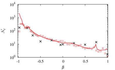
Figure 2: DSMC results for the relaxation times $\mathcal{N}_{r}^{\text{I}}$ and $\mathcal{N}_{r}^{\text{II}}$, as functions of the roughness parameter $\beta$, for a granular gas with $\alpha=0.9$ and $I=m\sigma^{2}/10$. The red line (Grad theory) and the squares (DSMC) stand for $\mathcal{N}_{r}^{\text{I}}$, as obtained in Ref. Vega Reyes et al. (2014) from the temperature ratio and the fourth-order cumulants. Crosses stand for $\mathcal{N}_{r}^{\text{II}}$, as extracted in the present work from the set of sixth- and eighth-order cumulants.

The two quantities $\mathcal{N}_{r}^{\text{I}}$ and $\mathcal{N}_{r}^{\text{II}}$ are compared in Fig. 2 for $\alpha=0.9$ and $-1\leq\beta\leq 1$. As can be seen, the results clearly show that, for the whole range of roughness $\beta$, $\mathcal{N}_{r}^{\text{II}}$ is not significantly different from $\mathcal{N}_{r}^{\text{I}}$. This implies that the global description of the relaxation to hydrodynamics in our previous work remains essentially the same. Thus, we can keep the conclusion that a hydrodynamic HCS is always reached for a granular gas of rough particles. It was also observed in Ref. Vega Reyes et al. (2014) that the values of $\mathcal{N}_{r}$ were rather insensitive to the degree of inelasticity (i.e., to the value of $\alpha$). Although we have not analyzed in Fig. 2 a value different from $\alpha=0.9$, the good agreement found in that case reinforces the latter observation. Figure 2 additionally shows that the relaxation time is relatively short ($\mathcal{N}_{r}\lesssim 10$) for the typical roughness values ($\beta\gtrsim 0$) of experimental relevance Louge (1999).

4.2 Stationary values

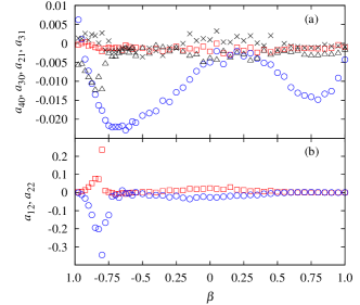
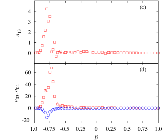
Figure 3: DSMC results for the stationary values of the sixth- and eighth-order cumulants, as functions of roughness $\beta$, for a granular gas with $\alpha=0.9$ and $I=m\sigma^{2}/10$. In panel (a), crosses, triangles, squares, and circles stand for $a_{30}$, $a_{21}$, $a_{40}$, and $a_{31}$, respectively. In panel (b), circles and squares stand for $a_{12}$ and $a_{22}$, respectively. In panel (d) circles and squares stand for $a_{03}$ and $a_{04}$, respectively.

It is interesting to note in Fig. 2 that the relaxation time tends to significantly grow in a roughness region close to the smooth limit $\beta\to-1$. One could expect that this signals a maximum in the magnitude of the asymptotic stationary values of the cumulants in the limit $\beta\to-1$, However, we saw in our previous work Vega Reyes et al. (2014) that the maxima actually occur before $\beta=-1$. This picture appears again in the stationary values of the higher-order cumulants analyzed in the present work, as we can see in Fig. 3. The magnitude of all these cumulants present a maximum value in a nearly-smooth region, and approximately at the same value of $\beta$ as in the case of the fourth-order cumulants. For $\alpha=0.9$ this occurs at $\beta\simeq-0.775$.

We can also observe that $|a_{03}|$ and $|a_{04}|$ reach maximum values that are significantly higher than the rest of cumulants. Those maxima are actually much higher than that of $|a_{02}|$, which is the largest fourth-order cumulant in the critical region. This result is important since it confirms that, at least in this special region of roughness values, the Maxwellian approximation dramatically fails. Actually, the result $|a_{04}|>|a_{03}|>|a_{02}|$ indicates that the polynomial expansion is not convergent Brilliantov and Pöschel (2006). Kinetic theories for granular gases are usually based on perturbative solutions around the Maxwellian and for all cases studied in the literature this approach works reasonably well Brilliantov and Pöschel (2000); Huthmann et al. (2000); Ahmad and Puri (2006, 2007); Santos and Montanero (2009). To the best of our knowledge, we report for the first time here and in Ref. Vega Reyes et al. (2014) such huge deviations from the Maxwellian for a homogeneous distribution of a granular gas.

5 Concluding remarks

Looking back at the results in the present work and in our previous work Vega Reyes et al. (2014), we may distinguish between two qualitatively different roughness regions in the HCS of a granular gas of inelastic rough hard spheres. First, a region where the velocity distribution function is weakly non-Maxwellian (WNM). In such a case, the distribution can be well represented by a Sonine polynomial series expansion around the Maxwellian and a linearized Grad approximation works well. We see from Fig. 3 that with $\alpha=0.9$ this WNM region corresponds to $-1\leq\beta\lesssim-0.9$ and $-0.6\lesssim\beta\leq 1$. In the complementary (and narrower) second region ($-0.9\lesssim\beta\lesssim-0.6$ if $\alpha=0.9$) the velocity distribution is strongly non-Maxwellian (SNM), especially in what concerns the distribution of angular velocities. Note that the SNM region was termed “critical” above. Figures 4(a) and 4(b) show representative examples of the velocity distribution function in the WNM and SNM regions, respectively.

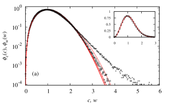
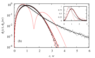
Figure 4: DSMC results (in logarithmic scale) for the marginal distribution functions $\phi_{c}(c)=4\pi c^{2}\int d\mathbf{w}\,\phi(\mathbf{c},\mathbf{w})$ ($\square$) and $\phi_{w}(w)=4\pi w^{2}\int d\mathbf{c}\,\phi(\mathbf{c},\mathbf{w})$ ($+$) at (a) $\alpha=0.7$, $\beta=0.5$ and (b) $\alpha=0.9$, $\beta=-0.75$. The solid lines stand for the (common) Maxwellian distribution function, while the dashed and dotted lines stand for the polynomial expansion (7) truncated after the fourth-order cumulants in the cases of $\phi_{c}(c)$ and $\phi_{w}(w)$, respectively. The insets show the distribution functions in normal scale.

Interestingly enough, as inelasticity increases (for instance, with $\alpha=0.7$), the SNM region widens and its non-Maxwellian features become less remarkable, while those of the WNM region become less negligible Vega Reyes et al. (2014). Therefore, an increase of inelasticity tends to smooth out the borders between the WNM and SNM regions. It is also worthwhile noting that orientational translational-rotational correlations, which imply $a_{00}^{(1)}\neq 0$ Brilliantov et al. (2007); Vega Reyes et al. (2014); Rongali and Alam (2014), are non-Maxwellian properties that are not especially large in the SNM region Vega Reyes et al. (2014).

While previous works already showed that the rough granular gas could be strongly non-Maxwellian Goldhirsch et al. (2005), only now really huge deviations have been measured and the complete spectrum of roughness values has been explored. Therefore, with our description of the fourth-order cumulants in our previous work Vega Reyes et al. (2014) and those of sixth- and eighth-order in the present work, we have a global picture of what the HCS velocity distribution function of the granular gas of rough spheres really looks like. Furthermore, the present results make now even more evident that the Maxwellian approximation does not work at all in a narrow interval of roughness values (what we called the SNM or critical region). This issue cannot be circumvented by just adding more terms in an expansion around the Maxwellian, as suggested recently Rongali and Alam (2014), since the series is likely not convergent, as we have shown. Outside the SNM region, this kind of Maxwellian-based approach still works. However, if we want to eventually attain a complete theoretical description of the velocity distribution function of this type of system, we would need to construct a novel approach.

On the other hand, and as we advanced, results in this work also confirm that the HCS hydrodynamic solution, whether or not close to a Maxwellian, is always attained. Furthermore, we can confirm that the aging time to hydrodynamics does not increase with increasing inelasticity (i.e., decreasing $\alpha$). This means that inelastic cooling alone, as long as the homogeneous base state lasts, does not break scale separation (i.e. that hydrodynamic fields variations continue to be slow compared to the microscopic reference time and length scales). This question is of interest since there has been concern about eventual restrictive effects of inelasticity over hydrodynamics. For instance, it sometimes has been used for the HCS an expansion in series of powers of the inelasticity (both for smooth and rough spheres) Sela and Goldhirsch (1998); Goldhirsch et al. (2005). As a consequence, the hydrodynamic solution is limited to the range of small inelasticities. In other cases, the Chapman-Enskog procedure is inherently limited to the quasi-elastic limit Jenkins and Richman (1985); Goldshtein and Shapiro (1995), based on the same concerns of lack of scale separation. However, the results in the present work and in Vega Reyes et al. (2014) help to clarify that scale separation occurs for the whole range of inelasticities in the HCS.

References

- Pauli (2000) W. Pauli, Pauli Lectures on Physics, vol. 4, Statistical Mechanics, Dover Publications, New York, 2000.
- Chapman and Cowling (1970) C. Chapman, and T. G. Cowling, The Mathematical Theory of Non-Uniform Gases, Cambridge University Press, Cambridge, UK, 1970, 3 edn.
- Batchelor (1953) G. K. Batchelor, The Theory of Homogeneous Turbulence, Cambridge University Press, Cambridge, UK, 1953.
- Batchelor (1967) G. K. Batchelor, An Introduction to Fluid Dynamics, Cambridge University Press, Cambridge, UK, 1967.
- Chaikin and Lubensky (2000) P. M. Chaikin, and T. C. Lubensky, Principles of Condensed Matter Physics, Cambridge University Press, Cambridge, UK, 2000.
- Goldhirsch (2003) I. Goldhirsch, Annu. Rev. Fluid Mech. 35, 267–293 (2003).
- Bagnold (1954) R. A. Bagnold, The Physics of Blown Sand and Desert Dunes, Dover Publications, Mineola, New York, 1954.
- Dufty and Brey (2011) J. W. Dufty, and J. J. Brey, Math. Model. Nat. Phenom. 6, 19–36 (2011).
- Jaeger et al. (1996) H. M. Jaeger, S. R. Nagel, and R. P. Behringer, Rev. Mod. Phys. 68, 1259–1273 (1996).
- Brilliantov and Pöschel (2004) N. V. Brilliantov, and T. Pöschel, Kinetic Theory of Granular Gases, Oxford University Press, Oxford, 2004.
- Garzó et al. (2007) V. Garzó, J. W. Dufty, and C. M. Hrenya, Phys. Rev. E 76, 031303 (2007).
- Vega Reyes et al. (2010) F. Vega Reyes, A. Santos, and V. Garzó, Phys. Rev. Lett. 104, 028001 (2010).
- Vega Reyes et al. (2014) F. Vega Reyes, A. Santos, and G. M. Kremer, Phys. Rev. E 89, 020202(R) (2014).
- Brilliantov et al. (2007) N. V. Brilliantov, T. Pöschel, W. T. Kranz, and A. Zippelius, Phys. Rev. Lett. 98, 128001 (2007).
- Goldhirsch et al. (2005) I. Goldhirsch, S. H. Noskowicz, and O. Bar-Lev, Phys. Rev. Lett. 95, 0682002 (2005).
- Santos et al. (2011) A. Santos, G. M. Kremer, and M. dos Santos, Phys. Fluids 23, 030604 (2011).
- Hansen and McDonald (2006) J.-P. Hansen, and I. R. McDonald, Theory of Simple Liquids, Academic Press, London, 2006.
- van Noije and Ernst (1998) T. P. C. van Noije, and M. H. Ernst, Granul. Matter 1, 57–64 (1998).
- Santos and Kremer (2012) A. Santos, and G. M. Kremer, “Relative Entropy of a Freely Cooling Granular Gas,” in 28th International Symposium on Rarefied Gas Dynamics 2012, edited by M. Mareschal, and A. Santos, AIP Conference Proceedings, Melville, NY, 2012, vol. 1501, pp. 1044–1050.
- Bird (1994) G. I. Bird, Molecular Gas Dynamics and the Direct Simulation of Gas Flows, Oxford University Press, Oxford, 1994.
- Louge (1999) M. Louge (1999), URL http://grainflowresearch.mae.cornell.edu/impact/data/Impact%20Results.html.
- Brilliantov and Pöschel (2006) N. Brilliantov, and T. Pöschel, Europhys. Lett. 74, 424–430 (2006).
- Brilliantov and Pöschel (2000) N. Brilliantov, and T. Pöschel, Phys. Rev. E 61, 2809–2812 (2000).
- Huthmann et al. (2000) M. Huthmann, J. A. G. Orza, and R. Brito, Granul. Matter 2, 189–199 (2000).
- Ahmad and Puri (2006) S. Ahmad, and S. Puri, Europhys. Lett. 75, 56–62 (2006).
- Ahmad and Puri (2007) S. Ahmad, and S. Puri, Phys. Rev. E 75, 031302 (2007).
- Santos and Montanero (2009) A. Santos, and J. M. Montanero, Granul. Matter 11, 157–168 (2009).
- Rongali and Alam (2014) R. Rongali, and M. Alam, Phys. Rev. E 89, 062201 (2014).
- Sela and Goldhirsch (1998) N. Sela, and I. Goldhirsch, J. Fluid Mech. 361, 41–74 (1998).
- Jenkins and Richman (1985) J. T. Jenkins, and M. W. Richman, Phys. Fluids 28, 3485–3494 (1985).
- Goldshtein and Shapiro (1995) A. Goldshtein, and M. Shapiro, J. Fluid Mech. 282, 75–114 (1995).