The loop-tree duality at work

Abstract:

We review the recent developments of the loop-tree duality method, focussing our discussion on analysing the singular behaviour of the loop integrand of the dual representation of one-loop integrals and scattering amplitudes. We show that within the loop-tree duality method there is a partial cancellation of singularities at the integrand level among the different components of the corresponding dual representation. The remaining threshold and infrared singularities are restricted to a finite region of the loop momentum space, which is of the size of the external momenta and can be mapped to the phase-space of real corrections to cancel the soft and collinear divergences.

1 Introduction

The recent discovery of the Higgs boson at the LHC represents a great success of the Standard Model (SM) of elementary particles. At the same time, the absence so far of a clear signal of physics beyond the SM during the first run of the LHC leaves a certain degree of dissatisfaction. Because of that, the high quality of data that the LHC will provide in the next run increases even more the relevance of high-precision theoretical predictions for the analysis of known phenomena and for finding innovative strategies to achieve new discoveries.

The loop-tree duality method [1, 2, 3, 4] establishes that generic loop quantities (loop integrals and scattering amplitudes) in any relativistic, local and unitary field theory can be written as a sum of tree-level objects obtained after making all possible cuts to the internal lines of the corresponding Feynman diagrams, with one single cut per loop and integrated over a measure that closely resembles the phase-space of the corresponding real corrections. This duality relation is realized by a modification of the customary +i0 prescription of the Feynman propagators. At one-loop, the new prescription compensates for the absence of multiple-cut contributions that appear in the Feynman Tree Theorem [5]. The modified phase-space raises the intriguing possibility that virtual and real corrections can be brought together under a common integral and treated with Monte Carlo techniques at the same time. In this talk, we review the actual state of development of the loop-tree duality method and focus our discussion on analysing the singular behaviour of the loop integrand of the dual representation of one-loop integrals and scattering amplitudes, as a necessary step towards a numerical implementation for the calculation of physical cross-sections.

2 The loop-tree duality relation at one-loop

The loop-tree duality relation is obtained by directly applying the Cauchy residue theorem to a general one-loop $N$-leg scalar integral

$$L^{(1)}(p_{1},\dots,p_{N})=\int_{\ell}\,\prod_{i\in\alpha_{1}}\,G_{F}(q_{i})~{},\quad\int_{\ell}\bullet=-i\int\frac{d^{d}\ell}{(2\pi)^{d}}\bullet~{},$$ (1)

where

$$G_{F}(q_{i})=\frac{1}{q_{i}^{2}-m_{i}^{2}+i0}$$ (2)

are Feynman propagators that depend on the loop momentum $\ell$, which flows anti-clockwise, and the four-momenta of the external legs $p_{i}$, $i\in\alpha_{1}=\{1,2,\ldots N\}$, which are taken as outgoing and are ordered clockwise (this kinematical configuration is shown in Fig. 1(left)). We use dimensional regularization with $d$ the number of space-time dimensions. The momenta of the internal lines $q_{i,\mu}=(q_{i,0},\mathbf{q}_{i})$, where $q_{i,0}$ is the energy (time component) and $\mathbf{q}_{i}$ are the spacial components, are defined as $q_{i}=\ell+k_{i}$ with $k_{i}=p_{1}+\ldots+p_{i}$, and $k_{N}=0$ by momentum conservation. We also define $k_{ji}=q_{j}-q_{i}$.

The dual representation of the scalar one-loop integral in Eq. (1) is thus the sum of $N$ dual integrals [1, 2]:

$$L^{(1)}(p_{1},\dots,p_{N}) = -\sum_{i\in\alpha_{1}}\,\int_{\ell}\;\tilde{\delta}\left(q_{i}\right)\,\prod_{\begin{subarray}{c}j\in\alpha_{1},j\neq i\end{subarray}}\,G_{D}(q_{i};q_{j})~{},$$ (3)

where

$$G_{D}(q_{i};q_{j})=\frac{1}{q_{j}^{2}-m_{j}^{2}-i0\,\eta\,k_{ji}}$$ (4)

are the so-called dual propagators, as defined in Ref. [1], with $\eta$ a future-like vector, $\eta^{2}\geq 0$, with positive definite energy $\eta_{0}>0$. The delta function $\tilde{\delta}\left(q_{i}\right)\equiv 2\pi\,i\,\theta(q_{i,0})\,\delta(q_{i}^{2}-m_{i}^{2})$ sets the internal lines on-shell by selecting the pole of the propagators with positive energy $q_{i,0}$ and negative imaginary part. The presence of the vector $\eta$ is a consequence of using the residue theorem and the fact that the residues at each of the poles are not Lorentz-invariant quantities. The Lorentz-invariance of the loop integral is recovered after summing over all the residues.

Figure 1: Momentum configuration of the one-loop (left) and two-loop (right) $N$-point scalar integrals.

3 Loop-tree duality relation at two-loops and beyond

The extension of the Duality theorem to two-loops and beyond has been discussed in detail in Ref. [2]. It is convenient to define the following functions combining different Feynman and dual propagators:

$$G_{F}(\alpha_{k})=\prod_{i\in\alpha_{k}}G_{F}(q_{i})~{},\qquad G_{D}(\alpha_{k})=\sum_{i\in\alpha_{k}}\,\tilde{\delta}\left(q_{i}\right)\,\prod_{\begin{subarray}{c}j\in\alpha_{k}\\ j\neq i\end{subarray}}\,G_{D}(q_{i};q_{j})~{},$$ (5)

where $\alpha_{k}$ is used to denote any set of internal momenta that depend on the same loop momentum or the sum of several independent loop momenta. At two loops we need three loop lines $\alpha_{k}$ to label all the internal momenta: $\alpha_{1}$, $\alpha_{2}$ and $\alpha_{3}$ for those momenta that depend on $\ell_{1}$, $\ell_{2}$ and $\ell_{1}+\ell_{2}$, respectively (see Fig. 1(right)). By definition $G_{D}(\alpha_{k})=\tilde{\delta}\left(q_{i}\right)$, when $\alpha_{k}=\{i\}$ consists of a single four-momentum. We also define:

$$G_{D}(-\alpha_{k})=\sum_{i\in\alpha_{k}}\,\tilde{\delta}\left(-q_{i}\right)\,\prod_{\begin{subarray}{c}j\in\alpha_{k}\\ j\neq i\end{subarray}}\,G_{D}(-q_{i};-q_{j})~{},$$ (6)

where the sign in front of $\alpha_{k}$ indicates that we have reversed the momentum flow of all the internal lines in $\alpha_{k}$.

The key ingredient necessary to extend the loop-tree duality theorem to higher orders is the following relationship relating the dual and Feynman functions of two subsets:

$$G_{D}(\alpha_{1}\cup\alpha_{2})=G_{D}(\alpha_{1})\,G_{D}(\alpha_{2})+G_{D}(\alpha_{1})\,G_{F}(\alpha_{2})+G_{F}(\alpha_{1})\,G_{D}(\alpha_{2})~{},$$ (7)

which can be generalized as well to the union of an arbitrary number of loop lines [2]. The application of the loop-tree duality theorem at higher orders proceeds in a recursive way. For the two-loop case, one starts by selecting one of the loops

$$L^{(2)}(p_{1},p_{2},\dots,p_{N}) = \int_{\ell_{1}}\,\int_{\ell_{2}}\,G_{F}(\alpha_{1}\cup\alpha_{2}\cup\alpha_{3})$$ (8)

$$= -\int_{\ell_{1}}\,\int_{\ell_{2}}\,G_{F}(\alpha_{2})\,G_{D}(\alpha_{1}\cup\alpha_{3})~{}.$$

As the loop-tree duality theorem applies to Feynman propagators only, we use Eq. (7) to re-express the dual propagators entering the second loop as Feynman propagators. The application of the loop-tree duality theorem to the second loop with momentum $\ell_{2}$ also requires to reverse the momentum flow in some of the loop lines. The final dual representation of a two-loop scalar integral reads:

$$L^{(2)}(p_{1},p_{2},\dots,p_{N}) = \int_{\ell_{1}}\int_{\ell_{2}}\,\{-G_{D}(\alpha_{1})\,G_{F}(\alpha_{2})\,G_{D}(\alpha_{3})$$

$$+ G_{D}(\alpha_{1})\,G_{D}(\alpha_{2}\cup\alpha_{3})+G_{D}(\alpha_{3})\,G_{D}(-\alpha_{1}\cup\alpha_{2})\}~{},$$

which is given by double cut contributions opening the loop diagram to a tree-level object.

4 The loop-tree duality relation for multiple poles

The appearance of identical propagators or powers of propagators can be avoided at one-loop by a convenient choice of the gauge [1], but not at higher orders. Identical propagators possess higher than single poles and the loop-tree duality theorem discussed so far, which is based on assuming single poles, must be extended to accommodate for this new feature. Two different strategies have been proposed in Ref. [3] to deal with this problem. The first one consists of extending the loop-tree duality theorem by using the Cauchy residue theorem for higher order poles. The second one consists of using Integration by Parts (IBP) [10, 11] to reduce integrals with multiple poles to integrals with single poles where the original loop-tree duality theorem can be applied directly. It is important to stress that in that case it is not necessary to perform a full reduction to a particular integral basis. Explicit examples at two- and three-loops have been presented in Ref. [3].

5 Cancellation of singularities among dual integrands

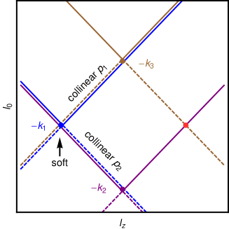
Figure 2: Light-cone hyperboloids for three arbitrary propagators in Cartesian coordinates in the ($\ell_{0}$,$\ell_{z}$) space (left). Kinematical configuration with infrared singularities (right).

Analysing the singular behaviour of the loop integrand in the loop momentum space is an attractive approach because it allows a rather direct physical interpretation of the singularities of the loop quantities [6]. This is particularly true for the case of the loop-tree duality method. The loop integrand becomes singular in regions of the loop momentum space in which subsets of internal lines go on-shell. In Cartesian coordinates, the Feynman propagator in Eq. (2) becomes singular at hyperboloids with origin in $-k_{i}$, where the minimal distance between each hyperboloid and its origin is determined by the internal mass $m_{i}$. This is illustrated in Fig. 2, where for simplicity we work in $d=2$ space-time dimensions. Figure 2 (left) shows a typical kinematical situation where two momenta, $k_{1}$ and $k_{2}$, are separated by a time-like distance, $k_{21}^{2}>0$, and a third momentum, $k_{3}$, is space-like separated with respect to the other two, $k_{31}^{2}<0$ and $k_{32}^{2}<0$. The forward light-cone hyperboloids ($q_{i,0}>0$) are represented in Fig. 2 by solid lines, and the backward light-cone hyperboloids ($q_{i,0}<0$) by dashed lines. The loop-tree duality method is equivalent to performing the loop integration along the forward light-cone hyperboloids. In the following, we take $\eta_{\mu}=(1,\mathbf{0})$, and thus $-i0\,\eta\,k_{ji}=-i0\,k_{ji,0}$.

Two or more Feynman propagators become simultaneously singular where their respective light-cone hyperboloids intersect. In most cases, these singularities, due to normal or anomalous thresholds [8, 9] of intermediate states, are integrable by contour deformation [7]. However, if two massless propagators are separated by a light-like distance, $k_{ji}^{2}=0$, then the overlap is tangential, as illustrated in Fig. 2 (right), and leads to non-integrable collinear singularities. In addition, massless propagators can generate soft singularities at $q_{i}=0$. In the dual representation of the integrand at least one propagator is already set on-shell, and we should analyse the singularities of the dual propagators. A crucial point of our discussion is the observation that dual propagators can be rewritten as

$$\tilde{\delta}\left(q_{i}\right)\,G_{D}(q_{i};q_{j})=i\,2\pi\,\frac{\delta(q_{i,0}-q_{i,0}^{(+)})}{2q_{i,0}^{(+)}}\,\frac{1}{(q_{i,0}^{(+)}+k_{ji,0})^{2}-(q_{j,0}^{(+)})^{2}}~{},$$ (10)

where

$$q_{i,0}^{(+)}=\sqrt{\mathbf{q}_{i}^{2}+m_{i}^{2}-i0}$$ (11)

is the loop energy measured along the light-cone hyperboloid with origin at $-k_{i}$. By definition we have ${\rm Re}(q_{i,0}^{(+)})\geq 0$. The factor $1/q_{i,0}^{(+)}$ can become singular for $m_{i}=0$, but the integral $\int_{\ell}\delta(q_{i,0}-q_{i,0}^{(+)})/q_{i,0}^{(+)}$ is still convergent by two powers in the infrared. For soft singularities to be generated two dual propagators, each one contributing with one power in the infrared, are required. From Eq. (10) it is obvious that dual propagators become singular, $G_{D}^{-1}(q_{i};q_{j})=0$, if one of the following conditions is fulfilled:

$$q_{i,0}^{(+)}+q_{j,0}^{(+)}+k_{ji,0}=0~{},$$ (12)

$$q_{i,0}^{(+)}-q_{j,0}^{(+)}+k_{ji,0}=0~{}.$$ (13)

The first condition, Eq. (12), is satisfied if the forward light-cone hyperboloid of $-k_{i}$ intersects with the backward light-cone hyperboloid of $-k_{j}$:

$$k_{ji}^{2}-(m_{j}+m_{i})^{2}\geq 0~{},\qquad k_{ji,0}<0~{},\qquad\rm{forward~{}with~{}backward~{}light-cones}~{}.$$ (14)

The second condition, Eq. (13), is true when the two forward light-cone hyperboloids intersect each other:

$$k_{ji}^{2}-(m_{j}-m_{i})^{2}\leq 0~{},\qquad\rm{two~{}forward~{}light-cones}~{}.$$ (15)

One of the main properties and advantages of the loop-tree duality method is that a partial cancellation of singularities occurs among different dual integrands [4]. For a qualitative discussion, let’s go back to Fig. 2 (left) where two of the Feynman propagators are separated by a space-like distance, $k_{31}^{2}<0$ (or more generally fulfilling Eq. (15)). In the corresponding dual representation one of these propagators is set on-shell while the other becomes dual, and the integration occurs along the respective forward light-cone hyperboloids. There, the two forward light-cone hyperboloids of $-k_{1}$ and $-k_{3}$ intersect at a single point. The integration over $\ell_{z}$ along the forward light-cone hyperboloid of $-k_{1}$ occurs outside the forward light-cone hyperboloid of $-k_{3}$ below the singular intersection point, and inside that light-cone above this point. The opposite occurs if we set $q_{3}$ on-shell; integration over $\ell_{z}$ happens from inside to outside the forward light-cone hyperboloid of $-k_{1}$. This leads to a change of sign and to the cancellation of the common singularity between the two dual contributions. Similarly, three and four space-like separated propagators do not lead to any common singularity. For a detailed analytic demonstration see Ref. [4]. If instead, the separation is time-like (in the sense of Eq. (14)), as is the case of $k_{2}$ with respect to $k_{1}$ in Fig. 2 (left), the common singularities are met only by one of the two forward light-cone hyperboloids, and then only one of the two dual integrands becomes singular.

A similar qualitative analysis is extensible to collinear singularities, occurring when two massless propagators are separated by a light-like distance, e.g. $k_{31}^{2}=0$ in Fig. 2 (right). In that case, the corresponding light-cone hyperboloids overlap tangentially along an infinite interval. The collinear singularity for $\ell_{0}>-k_{3,0}$, however, appears at the intersection of the two forward light-cone hyperboloids, with the forward light-cone hyperboloid of $-k_{3}$ located inside the forward light-cone hyperboloid of $-k_{1}$, equivalently with the forward light-cone hyperboloid of $-k_{1}$ located outside the forward light-cone hyperboloid of $-k_{3}$, and then the singularities cancel each other. For $-k_{1,0}<\ell_{0}<-k_{3,0}$, instead, it is the forward light-cone hyperboloid of $-k_{1}$ that intersects tangentially with the backward light-cone hyperboloid of $-k_{3}$ according to Eq. (12). The collinear divergences survive in this energy strip, which indeed also limits the range of the loop three-momentum. The soft singularity of the integrand at $q_{i,0}^{(+)}=0$ leads to soft divergences only if two other propagators, each one contributing with one power in the infrared, are light-like separated from $-k_{i}$. In Fig. 2 (right) this condition is fulfilled at $q_{1,0}^{(+)}=0$ only.

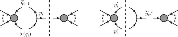
Figure 3: Factorization of the dual one-loop and tree-level squared amplitudes in the collinear limit. The dashed line represents the momentum conservation cut.

6 Cancellation of infrared singularities with real corrections

In the previous section we have seen that both threshold and infrared singularities are constrained in the dual representation of the loop integrand to a finite region of the loop three-momentum. Singularities outside this region, occurring in the intersection of forward light-cone hyperboloids, cancel in the sum of all the dual contributions. The size of this region is of the order of the external momenta, and can be mapped to the finite-size phase-space of the real corrections. To discuss the cancellation of infrared singularities with the real corrections we make use of collinear factorization and the splitting matrices, which encode the collinear singular behaviour of scattering amplitudes, as introduced in Ref. [12]. We consider the one-loop scattering amplitude ${\cal M}^{(1)}_{N}$ with the internal momenta $q_{i}$ on-shell and the limit where $\mathbf{p}_{i}$ and $\mathbf{q}_{i}$ become collinear

$$|{{\cal M}^{(0)}_{N}(p_{1},\ldots,p_{N})}\rangle \to |{{\cal M}^{(0)}_{N+2}(\ldots,p_{i},-q_{i},q_{i},p_{i+1},\ldots)}\rangle$$

$$= {\mathbf{Sp}}^{(0)}(p_{i},-q_{i};-\widetilde{q}_{i-1})\,|{\overline{\cal M}^{(0)}_{N+1}(\ldots,p_{i-1},-\widetilde{q}_{i-1},q_{i},p_{i+1},\ldots)}\rangle+{\cal O}(q_{i-1}^{2})~{},$$

where the reduced matrix element $\overline{\cal M}^{(0)}_{N+1}$ is obtained by replacing the two collinear partons of ${\cal M}^{(0)}_{N+2}$ by a single parent parton with light-like momentum $\widetilde{q}_{i-1}^{\mu}=q_{i-1}^{\mu}-\frac{q_{i-1}^{2}\,n^{\mu}}{2\,nq_{i-1}}$, with $n^{2}=0$. Its interference with the corresponding $N$-parton tree-level scattering amplitude ${\cal M}^{(0)}_{N}$, is integrated with the appropriate phase-space factor

$$\int d\Phi_{N}(p_{1};p_{2},\ldots,p_{N})=\left(\prod_{i=2}^{N}\int_{p_{i}}\tilde{\delta}\left(p_{i}\right)\right)\,\delta^{(d)}(\sum_{i=1}^{N}p_{i})\,\theta(p_{i,0}-q_{i,0}^{(+)})~{},$$ (17)

where we assume that only the external momentum $p_{1}$ is incoming ($p_{1,0}<0$). Notice that the loop energy in Eq. (17) is restricted by the energy of the external particle $p_{i}$ because we have selected the infrared divergent region. This restriction allows for the mapping with real corrections, as illustrated in Eq. (3).

Similarly, we consider the $N+1$ tree-level scattering amplitude where the parton $i$ radiates an extra parton $r$. Besides the initial state momentum $p_{1}$, we denote the external momenta of the real corrections as primed momenta because they are subject to the momentum conservation delta function. In the limit where $\mathbf{p}_{i}^{\prime}$ and $\mathbf{p}_{r}^{\prime}$ become collinear, ${\cal M}^{(0)}_{N+1}$ factorizes as

$$\langle{{\cal M}^{(0)}_{N+1}(p_{1},\ldots,p_{N+1}^{\prime})}|=\langle{\overline{\cal M}^{(0)}_{N}(\ldots,p_{i-1}^{\prime},\widetilde{p}_{ir}^{\prime},p_{i+1}^{\prime},\ldots)}|\,{\mathbf{Sp}}^{(0)\dagger}(p_{i}^{\prime},p_{r}^{\prime};\widetilde{p}_{ir}^{\prime})+{\cal O}(s_{ir}^{\prime})~{},$$ (18)

where $p_{ir}^{\prime}=p_{i}^{\prime}+p_{r}^{\prime}$, $s_{ir}^{\prime}=p_{ir}^{\prime 2}$, and $\widetilde{p}_{ir}^{\prime\mu}=p_{ir}^{\prime\mu}-\frac{s_{ir}^{\prime}\,n^{\mu}}{2\,np_{ir}^{\prime}}$. As Fig. 3 suggests the mapping between the four-momenta of the virtual and real matrix elements should be such that $p_{i}=\widetilde{p}_{ir}^{\prime}$, $p_{j}=p_{j}^{\prime}(j\neq i)$, $-\widetilde{q}_{i-1}=p_{i}^{\prime}$ and $q_{i}=p_{r}^{\prime}$, in the collinear limit. For more details see Ref. [4].

7 Conclusions and outlook

The loop-tree duality method presents quite attractive features for the calculation of multipartonic cross-sections at higher orders. Integrand singularities occurring in the intersection of forward light-cones, or equivalently from space-like separated propagators, cancel among dual integrals. The remaining singularities, excluding UV divergences, are found in the intersection of forward with backward light-cones and are produced by dual propagators that are time-like separated (or causally connected) and less energetic than the internal propagator that is set on-shell. Therefore, these singularities are restricted to a finite region of the loop three-momentum space, which is of the size of the external momenta. As a result, a local mapping at the integrand level is possible between one-loop and tree-level matrix elements to cancel soft and collinear divergences. One can anticipate that a similar analysis at higher orders of the loop-tree duality relation is expected to provide equally interesting results.

Acknowledgements: We thank S. Catani for a fruitful long-term collaboration. This work has been supported by the EU under the Grant Agreement PITN-GA-2010-264564 (LHCPhenoNet), the Spanish Government and EU ERDF funds (FPA2011-23778 and CSD2007-00042 CPAN) and GV (PROMETEUII/2013/007). SB acknowledges support from JAEPre (CSIC). GC from Marie Curie Actions (PIEF-GA-2011-298582). IB acknowledges support from the German Science Foundation (DFG) within the Collaborative Research Centre 676 “Particles, Strings and the Early Universe”.

References

- [1] S. Catani, T. Gleisberg, F. Krauss, G. Rodrigo and J. C. Winter, JHEP 0809 (2008) 065.
- [2] I. Bierenbaum, S. Catani, P. Draggiotis and G. Rodrigo, JHEP 1010 (2010) 073.
- [3] I. Bierenbaum, S. Buchta, P. Draggiotis, I. Malamos and G. Rodrigo, JHEP 1303 (2013) 025. I. Bierenbaum et al., Acta Phys. Polon. B 44 (2013) 11, 2207.
- [4] S. Buchta, G. Chachamis, P. Draggiotis, I. Malamos and G. Rodrigo, arXiv:1405.7850 [hep-ph].
- [5] R. P. Feynman, Acta Phys. Polon. 24 (1963) 697;
- [6] G. F. Sterman, Phys. Rev. D 17 (1978) 2773.
- [7] D. E. Soper, Phys. Rev. Lett. 81 (1998) 2638.
- [8] S. Mandelstam, Phys. Rev. Lett. 4 (1960) 84.
- [9] H. Rechenberg and E. C. G. Sudarshan, Nuovo Cim. A 12 (1972) 541.
- [10] K. G. Chetyrkin and F. V. Tkachov, Nucl. Phys. B 192 (1981) 159.
- [11] V.A. Smirnov, Feynman Integral Calculus, Springer-Verlag (2006)
- [12] S. Catani, D. de Florian and G. Rodrigo, Phys. Lett. B 586 (2004) 323. G. F. R. Sborlini, D. de Florian and G. Rodrigo, JHEP 1401 (2014) 018.