Scalar suppression on large scales in open inflation
Abstract
We consider two toy models of open inflation and investigate their ability to give a suppression of scalar power on large scales whilst also satisfying observational constraints on the spatial curvature of the universe. Qualitatively we find that both models are indeed capable of fulfilling these two requirements, but we also see that effects of the quantum tunnelling must be carefully taken into account if we wish to make quantitative predictions.
pacs:
98.80.CqI Introduction
Precision measurements of the cosmic microwave background (CMB) by the WMAP and Planck collaborations are in very good agreement with what has become the standard model of cosmology, namely inflation plus CDM Hinshaw et al. (2013); Ade et al. (2013a, b). There are, however, some anomalies, such as a 5–10% deficit in the temperature power spectrum on large scales () Ade et al. (2013c). Whilst the statistical significance of this anomaly is currently only –, the tension will be exacerbated if the recent findings of the BICEP2 team – who have reported a tensor-to-scalar ratio of Ade et al. (2014) – are confirmed Bousso et al. (2014); Smith et al. (2014). The reason for this increased tension is easy to understand: the temperature power spectrum on large scales () receives contributions from both scalar and tensor perturbations, meaning that for a given observed power the scalar contribution must be suppressed if there exists a non-negligible tensor contribution.
Perhaps the simplest way in which a suppression on large scales can be accommodated is to allow for a negative running of the spectral index, defined as . What one finds, however, is that the required value of is , Ade et al. (2014); Abazajian et al. (2014), which is one or two orders of magnitude larger than the running predicted in standard slow-roll models of inflation. Moreover, a large running also tends to spoil the fit to data on small scales. As such, it appears that a non-power-law scalar spectrum may be preferred Abazajian et al. (2014); Hazra et al. (2014a), namely one that is able to give a localised suppression on large scales. Note that one can also try to alleviate tensions between the BICEP2 results and those of Planck by allowing for a modified tensor spectrum Smith et al. (2014); Gong (2014); Gerbino et al. (2014), but here we focus on modifying the scalar spectrum.
In canonical single-field models of inflation the power spectrum takes the simple form
| (1) |
where the subscript denotes the fact that the quantity should be evaluated at the time when the scale left the Hubble horizon. Given the inverse dependence on , a natural way in which we might seek to suppress the spectrum would be to require that the field be rolling quickly during the period that large scales left the horizon, i.e. during the first few observable e-foldings of inflation.111Note that there are other possible mechanisms, see e.g. Contaldi et al. (2003); Cline et al. (2003); Powell and Kinney (2007); Kawasaki et al. (2014). This mechanism for suppression has been considered in the literature, see e.g. Contaldi et al. (2003); Jain et al. (2009); *Jain:2009pm; Pedro and Westphal (2014); Hazra et al. (2014b), and in canonical single-field inflation models an enhancement of is associated with a steepening of the potential towards the onset of inflation. Whilst such a tuned steepening might seem unnatural, this is not necessarily the case in the context of open inflation Bousso et al. (2013, 2014); Freivogel et al. (2006, 2014); Linde (1999); Linde et al. (1999).
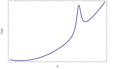
Models of open inflation involve potentials of the form shown in figure 1, and the last stage of observable inflation is preceded by tunnelling from a false vacuum described by a Coleman-De Luccia (CDL) instanton Coleman and De Luccia (1980). The universe nucleated in the tunnelling process has negative curvature, i.e. it is open. In general, CDL instantons require during the tunnelling process Jensen and Steinhardt (1984), which is in contradiction with the requirement for slow-roll inflation. As such, it is expected that between the end of the tunnelling process and the onset of standard slow-roll inflation one has an intervening stage of “fast-roll” inflation, during which the potential becomes progressively less steep. In order that observable signatures of this fast-roll phase remain, we require that the ensuing stage of slow-roll inflation does not last too long. If the number of e-foldings is too small, however, then the model becomes tightly constrained by observational constraints on today. The compatibility of these two competing effects was discussed by Freivogel et al. and Bousso et al. Freivogel et al. (2006, 2014); Bousso et al. (2013, 2014). It was found that models providing sufficient suppression of the scalar spectrum whilst satisfying bounds on are possible if the steepening of the potential towards the barrier is gradual enough.
In this paper we revisit the toy models of open inflation presented in Linde (1999) and Linde et al. (1999), and investigate their ability to produce a suppression of the large-scale scalar spectrum whilst evading observational constraints on . In section II we begin by giving a brief summary of open inflation and present the relevant background and perturbation equations. In section III we then analyse two of the toy models discussed in Linde (1999). Based on the two toy models, in section IV we then summarise more generally the nature of suppression from open inflation models and how they can be constrained using observations. Finally we conclude in section V
II Open inflation
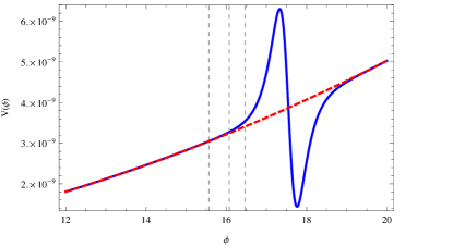
To describe the tunnelling process preceding single-field open inflation, we consider a class of model whose effective potential has a local minimal at and global minimum at with , as depicted in figure 1. The action is given by
| (2) |
Note that here and throughout the paper we set .
Conventionally, the instanton solution is explored under the assumption of symmetry, since it has been proved that the -symmetric solution gives the lowest value of the Euclidean action for a wide class of scalar-field theories Coleman et al. (1978). Hence, this solution is exponentially favoured when calculating the corresponding tunnelling probability. It is also reasonable to use this assumption with gravity included Coleman and De Luccia (1980). To be specific, the metric of an -invariant Euclidean spacetime can be written as
| (3) |
The corresponding Euclidean background equations are given as
| (4) | |||||
| (5) |
where a dot denotes differentiation with respect to and . For the CDL instanton solution, we choose to coincide with the centre of the nucleated -symmetric bubble, at which , and . We further set () in the false vacuum, where , and .
On making an analytic continuation to the Lorentzian space corresponding to our open universe, the metric takes the form Sasaki et al. (1995, 1995); Yamauchi et al. (2011); Sugimura and Komatsu (2013)
| (6) |
where , , and , and the background equations of motion become
| (7) | |||
| (8) |
where a dot now denotes taking the derivative with respect to . The initial conditions coming from the instanton solution are , , and . Using these equations of motion and initial conditions, we then need to solve for the ensuing inflationary dynamics.
Locating the observer at the centre of the spherical coordinates, the only tensor modes that contribute to the CMB temperature power spectrum are the even-parity modes, which can be expressed as
| (9) |
Here are the annihilation operators, are the even-parity tensor harmonics on a unit 3-hyperboloid and is the conformal time. The are found to satisfy Garriga et al. (1999)
| (10) |
where a prime denotes and .
The important scalar quantity is the comoving curvature perturbation , but this is more conveniently expressed in terms of a new variable as
| (11) |
The variable then satisfies the simple equation
| (12) |
The scalar and tensor power spectra are given in terms of and as
| (13) |
respectively. In this work we fit the power spectra using the following functional forms:
| (14) | ||||
| (15) |
where the subscripts and indicate that the quantity should be evaluated at the horizon-crossing time for scalar and tensor modes, respectively. The phase is irrelevant for large and behaves as for . In fact, we take throughout, which corresponds to the case where maximal suppression is achieved. The above expressions for and are based on analytic approximations derived in Yamamoto et al. (1996); Garriga et al. (1999). We can see that they differ from the standard expressions by the -dependent “suppression factors,” which tend to unity for large and for . This -dependent suppression is distinct from that associated with the fast-roll dynamics, and reflects the systems memory of the quantum tunnelling that preceded inflation Linde et al. (1999). The parameters and determine the scales at which this additional suppression becomes active for the scalar and tensor modes, respectively. Under the weak back-reaction approximation, the spectra were found to take the above form with and Yamamoto et al. (1996); Garriga et al. (1999). In Appendix C of Garriga et al. (1999), similar expressions were also found for an analytically soluble model, but with and . In this paper we take the two parameters and as free parameters that we use to fit the numerical results of Linde et al. (1999).
In order to determine the horizon-crossing conditions we return to the equations of motion. Firstly, for , we see from (10) that horizon crossing takes place when , as in the standard case. In order to determine , we first need to use (11) and (12) to find an equation of motion for . We find222This equation can also be derived using the action for given in Appendix B of Garriga et al. (1998).
| (16) |
with
| (17) | ||||
| (18) |
where . Note that in the limit of large ( large ) the equation of motion for reduces to the standard form, where, defining , and . Defining horizon crossing as when , noting and assuming and (which is always the case after curvature domination in our particular models), we find the condition
| (19) |
One can see that if the slow-roll condition is satisfied, then this reduces to the standard horizon-crossing condition for large .
III Toy Models
Having summarised the key features of open inflation models and the relevant background and perturbation equations, in this section we revisit two of the toy models that were introduced and analysed numerically in Linde et al. (1999).
III.1 Model 1
The potential of Model 1 takes the form
| (20) |
We consider the same parameter values as considered in Linde et al. (1999), except we work in reduced Planckian units instead of Planckian units. As such, our parameters are given as
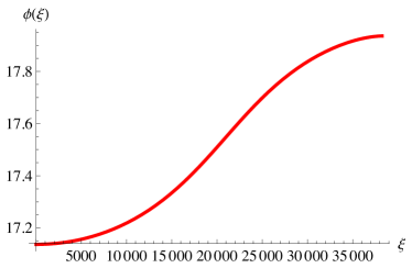
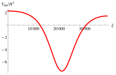
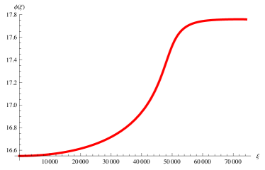
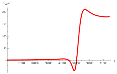
By solving Eqs. (4) and (5) numerically, one is able to find a CDL instanton solution, which is plotted in the upper panel of figure 2. The value of the field at the end of the tunnelling is given as
| (21) |
In the lower panel of figure 2 we plot along the CDL instanton trajectory, and we see that is indeed satisfied for most of the trajectory.
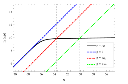
Using the value of found above, we then solve the background equations of motion (7) and (8) for and after the tunnelling. In figure 3 we plot the resulting evolution of the Hubble parameter as a function of the number of e-foldings before the end of inflation (solid black curve).333The end of inflation is taken to be when . We also plot three scales of interest, which are
-
1.
the curvature scale, corresponding to (blue dashed curve),
-
2.
the upper limit on the current Hubble scale, as determined by the constraint , i.e. (red dot-dashed curve), and
-
3.
the scale that approximately corresponds to the CMB multipole , as determined assuming that is given by the upper limit mentioned above (green dotted curve).
Finally, the times at which the last two of the aforementioned scales leave the horizon (as simply determined by ) are marked with vertical dashed lines approximately 64 and 60 e-foldings before the end of inflation, respectively. The third, left-most vertical dashed line, located approximately 66 e-foldings before the end of inflation, corresponds to the time of potential-curvature equality. Unless otherwise mentioned, the vertical dashed lines shown in all following plots will correspond to these same three events. As we will see later, it is also important to know the time at which the curvature becomes sub-dominant to the kinetic component of . Interestingly, in Model 1 this time almost exactly coincides with the time at which the scale left the horizon, i.e. e-foldings before the end of inflation. The evolution of the three components of are plotted explicitly in figure 4.
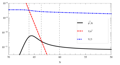
We emphasise that the discussed above corresponds to the current Hubble scale as determined assuming that the observational constraint on is saturated. For our choice of model parameters, we see that this scale would leave the horizon approximately e-foldings before the end of inflation. However, this would seem a little too early, as standard arguments dictate that the current horizon scale left the horizon e-foldings before the end of inflation Liddle and Leach (2003).
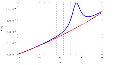
In order to help relate features in the background dynamics and power spectrum to the underlying potential, in figure 5 we indicate the location of the scalar field on the potential at the three times discussed above. Note that the order of the vertical dashed lines is the reverse of that in other plots. Looking at the form of the potential (20), we see that it naturally lends itself to being decomposed into a fiducial potential and a correction to this around the tunnelling barrier. As such, in figure 5 we also plot the fiducial potential. We see that the steepening of the potential relative to remains non-negligible until after the scale leaves the horizon. As such, we expect that observable scales will indeed be subject to suppression in this model.
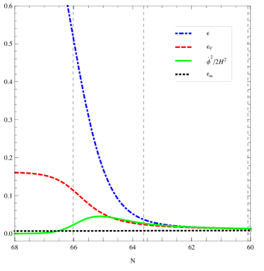
In the upper panel of figure 6 we compare the evolution of the three slow-roll parameters , and with the evolution of . As we can see from (14), the quantity that we are interested in evaluating is . In the case of a flat universe, this can be re-expressed in terms of as , which in turn, under the slow-roll approximation can be re-expressed as . In the case of open inflation, however, we have , meaning that we can no longer directly replace with . Moreover, as the slow-roll condition may be violated in the early stages of evolution after tunnelling, we are also not necessarily able to make the second approximation . Of course, at late times we expect the curvature to become negligible and for slow-roll inflation to take place, so it is interesting to explicitly see at what stage the equivalence of the three quantities is recovered. As we can see from figure 6, the equivalence is recovered approximately e-foldings before the end of inflation. This time is shortly after that at which the curvature term becomes negligible in comparison to both the potential and kinetic terms in the Friedmann equation. This is exactly as we would expect in light of the contribution of to . The fact that and also become approximately equal at this time tells us that the potential must already be relatively flat and the slow-roll approximation is a good one. Another point to note from this figure is the difference between and at early times. As a result of the initial conditions imposed by the CDL instanton and the initial curvature domination, asymptotes to unity whilst vanishes. This is evidently very important in determining the asymptotic behaviour of , as we will see shortly. Finally the that we have plotted corresponds to the slow-roll parameter associated with the fiducial potential. We can see that even 60 e-foldings before the end of inflation there is a non-negligible difference between and .
To leading order in the slow-roll approximation, the tilt of the power spectrum is given as
| (22) |
where . Using the fact that , this can be written in the perhaps more familiar form
| (23) |
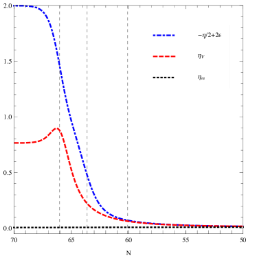
We know that the initial conditions prescribed by the CDL instanton dictate that be large, which will tend to give a blue-tilted spectrum. Given that the spectrum must be red-tilted on small scales, we are therefore interested in following the evolution of and in determining when the transition from a blue- to a red-tilted spectrum takes place. As such, in the lower panel of figure 6 we plot the evolution of , and , where the last quantity corresponds to the equivalent slow-roll parameter associated with the fiducial potential. Similar to the case with and , we note the different behaviour of and at early times. This is again due to the initial conditions imposed by the CDL instanton and the domination of curvature, which give and as . Comparing with the upper panel of figure 6, we also note that the time at which the three different definitions of become equivalent is somewhat later than the corresponding time for .
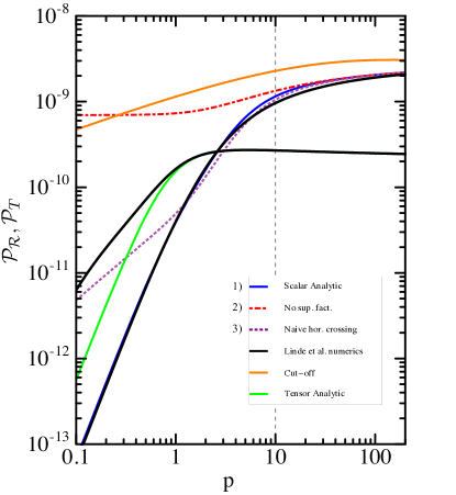
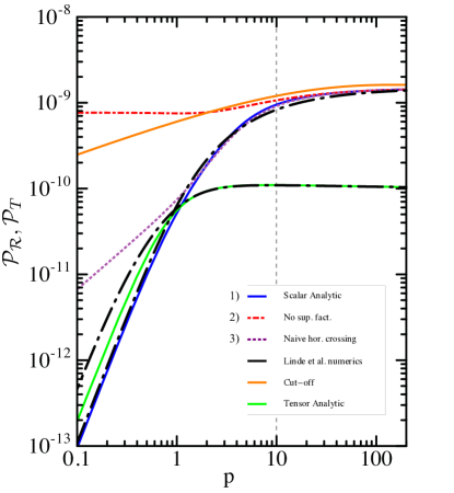
In figure 7 we plot the scalar and tensor power spectra associated with Model 1 as functions of the comoving scale . In the case of the scalar spectrum we plot four different curves. Three of these correspond to different variants of the analytic expression (14), namely 1) the full expression (14) (blue solid curve) 2) (14) without the -dependent suppression factor that distinguishes (14) from the standard flat-universe expression (red dot-dashed curve) and 3) (14) taking as the time when instead of when the condition (19) is satisfied (purple dotted curve). The upper solid black curve then corresponds to the numerical solution for found in Linde et al. (1999). We take in (14), which we find to give the best fit to the numerical results for small . Qualitatively, we see that the full analytic result (solid blue curve) matches the numerics well, especially for small and large . At intermediate scales, around , however, it tends to underestimate the amount of suppression, with the discrepancy being on the order of 10%. If we assume that the observational bound on is saturated, this scale coincides exactly with the current Horizon scale. As such, if we are interested in quantitatively constraining the suppression from open inflation, we see that numerical calculations are necessary.
From curves 2) and 3) we are able to appreciate the importance of corrections to the standard flat-universe expression for for small . The fact that curve 2) always underestimates the suppression of the scalar spectrum highlights the fact that the fast-rolling of the inflaton is not the only source of suppression, especially on very large scales. The additional suppression reflects the system’s memory of the tunnelling process preceding inflation Linde et al. (1999). We also see that curve 3) underestimates the suppression for . This reflects the fact that large-scale modes freeze out at later times than predicted by the standard horizon-crossing condition, leading to a suppression in their amplitude. As expected, all curves converge for large , where the effects of the tunnelling become negligible.
In addition to the four curves discussed above, for comparison we also plot the spectrum associated with the so-called cut-off model that has been considered in the literature, see e.g. Contaldi et al. (2003); Cline et al. (2003). The model – corresponding to the solid orange curve in figure 7 – is a phenomenological example of a spectrum with suppression on large scales, and takes the form
| (24) |
The Planck team found that such a form for the spectrum was preferred over power-law CDM with Ade et al. (2013b). The corresponding best-fit parameters were and , where the pivot scale was used. Whilst it is not our intention that our models quantitatively fit the data well, it is nevertheless interesting to qualitatively compare our spectra with this cut-off model. For the orange curve in figure 7 we have used Planck’s best-fit values for and and further assumed that and . The amplitude is adjusted so that our spectrum and the phenomenological model agree at , as both spectra have relaxed to the standard power-law form on these scales.
In comparing Model 1 with the cut-off spectrum, the main feature we note is that Model 1 gives substantially more suppression. This feature is favourable in light of the fact that Planck’s best-fit spectrum was found assuming no tensor modes. In order to be able to accommodate a tensor contribution to large-scale CMB temperature fluctuations (as suggested by BICEP2), we expect that a larger suppression of the scalar spectrum will be required. The discrepancy between the two models is, however, rather substantial, even at . Better agreement could perhaps be achieved by correcting our assumption that . As such, in Model 1 we may find that the best-fit value for is unobservably small.
For reference, we also plot the tensor spectrum, but this time only include the full analytic result given by (15) with (solid green curve) and the numerical results from Linde et al. (1999) (lower solid black curve). It is clear to see that the onset of suppression occurs at much smaller in the case of the tensor spectrum, i.e. on scales larger than the current Hubble horizon. In contrast with the scalar spectrum, the tensor spectrum is not affected by the fast rolling of the inflaton. As such, the suppression on large scales is purely a result of the pre-inflationary tunnelling and the presence of the bubble wall. See Linde et al. (1999) for a more detailed discussion.
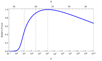
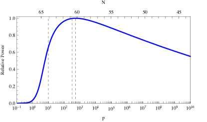
Finally, in figure 8 we plot the magnitude of the scalar power relative to that at the scale at which the spectrum transitions from being blue- to red-tilted. This transition occurs approximately 56 e-foldings before the end of inflation, when the scale left the horizon. Given that potential-curvature equality occurs approximately 66 e-foldings before the end of inflation, we find that we have roughly 10 e-foldings of the “fast roll” phase before the spectrum becomes red-tilted and standard slow-roll is achieved.
Even in the best-case scenario, it is only possible to detect a , which would correspond to . As such, we see that in Model 1 we have the possibility that suppression of the scalar spectrum is observed on large scales whilst remains undetectable. Indeed, if we were to make the usual assumption that leaves the horizon e-foldings before the end of inflation, this would correspond to , giving an unobservable . However, in such a scenario the scale would coincide with , and suppression on the order of 10% would be observed at scales corresponding to the current Hubble horizon.
III.2 Model 2
The second model considered in Linde et al. (1999) has a potential of the form
| (25) |
with parameters chosen as
The CDL instanton solution and the evolution of through the tunnelling process are shown in figure 9. From the upper plot we are able to obtain , and from the lower plot we see that the condition is indeed satisfied for most of the trajectory.
Qualitatively, the features of Model 2 are very similar to Model 1, except that the dependence of the potential on hyperbolic trigonometric functions makes deviations from the fiducial potential around the tunnelling barrier sharper and more localised. Given the similarities, we refrain from reproducing the full set of plots given in the case of Model 1, focusing only on those we feel highlight the differences between the two models.
In order to highlight the sharpness of the barrier feature, in figure 10 we plot Model 2’s equivalent of figure 5. Namely, we plot the potential, the corresponding fiducial potential and the position of the field at the time of potential-curvature equality, the time that left the horizon and the time that left the horizon. We see that the potential relaxes to the fiducial one at around the time that left the horizon, which is much sooner than in the case of Model 1. As such, we expect that a much smaller range of scales will be subject to suppression.
In figure 11 we plot the scalar and tensor power spectra as a function of , with the same set of curves included here as in figure 7. Regarding the scalar spectrum, in the case of Model 2 we find that using in (14) gives a better fit to the numerical results of Linde et al. for small . Once again we find that at intermediate scales, i.e. , the analytic fit differs from the numerical results by an amount on the order of 10%. We also see that neglecting the -dependent suppression factor in (14) and using only the naive horizon-crossing condition to determine have very similar effects as in the case of Model 1. The cut-off spectrum represented by the solid orange curve is constructed in exactly the same way as in the case of Model 1. As with Model 1, we find that the spectrum of Model 2 is much more suppressed on large scales compared to the cut-off model. A tensor contribution to CMB temperature fluctuations could therefore be accommodated in the case that the results of BICEP2 are confirmed. In comparison with Model 1, Model 2 is in much better agreement with the cut-off spectrum on smaller scales. Regarding the tensor spectrum, we once again use in our fit, and again we can see that suppression of the tensor spectrum only becomes active at much lower than in the case of the scalar spectrum.
Finally, in figure 12 we plot the magnitude of the scalar power spectrum relative to its value at the scale of the transition between a blue- and a red-tilted spectrum. It is in this plot that the differences between Models 1 and 2 become most apparent. Comparing with figure 8 we see that the transition from a blue- to a red-tilted spectrum occurs a few e-foldings earlier in Model 2, approximately 60 e-foldings before the end of inflation. Given that potential-curvature equality occurs approximately 66 e-foldings before the end of inflation, this means that we only have around 6 e-foldings of the “fast-roll” phase. Correspondingly, a suppression of the scalar power spectrum is observable over a much smaller range of scales, with the smallest affected scales being quite close to in the case that . Nevertheless, the model is still able to give rise to a suppression on observationally relevant scales whilst also satisfying constraints on . Unlike Model 1, however, we see that if is of non-detectable magnitude, i.e. , then this model likely gives no suppression on observable scales. Similarly, if we were to make the standard assumption that the current Hubble scale left the horizon e-foldings before the end of inflation, then we see that there would be no suppression on observable scales.
IV General constraints
As discussed in the introduction, our motivation for considering open inflation models is that they naturally give rise to a fast-roll phase between tunnelling from the false vacuum and the onset of slow-roll inflation, which in turn leads to a suppression of the scalar power spectrum for modes leaving the horizon during this period. However, in order for this suppression to be observable, we require that the total number of e-foldings of inflation be relatively small. This in turn means that the curvature of space may not get diluted enough to satisfy current observational constraints on . In this section we summarise how observational constraints on these two competing effects might be used to constrain models of open inflation.
As confirmed in the toy models of the preceding section, in general we expect that the dynamics can be considered in three stages. The first is the curvature-dominated stage, where , such that and . During this stage the Hubble friction term is large, meaning that is very small. After the time , defined by , the potential energy comes to dominate over the curvature term. In the initial potential-dominated stage the slope of the potential may still be somewhat steeper than usually dictated by the requirement for slow roll. As such, in this stage we might expect to be somewhat enhanced, leading to a suppression of the scalar power spectrum for modes leaving the horizon during this period. Finally, as the field evolves away from the barrier, the potential flattens and usual slow-roll inflation occurs. The above scenario is depicted schematically in figure 13.

In addition to the evolution of the Hubble parameter, figure 13 shows the evolution of the physical length scales associated with the curvature scale, , the current Hubble scale, , and the scale associated with the onset of power suppression, . These scales can all be constrained using observations, which allows us to determine the relative position of the corresponding curves on the plot. For a given open inflation model, we would then require that the time at which the scale associated with the onset of suppression leaves the horizon coincides with the onset of slow-roll inflation.
To determine the separation between the curvature scale and the current Hubble scale, we note that the current observational constraint on is . We therefore find , which corresponds to the vertical spacing between the blue and red lines in figure 13.
Next, in order to determine an estimate for the separation between the current Hubble scale and the scale at which the onset of scalar suppression is observed, we use the results of a recent analysis by Easther et al. Abazajian et al. (2014). In this work they considered a “broken” spectrum that is red-tilted up to some given scale and then blue-tilted for larger scales, thus explaining the suppression on large scales. The transition is assumed to take place instantaneously at , and the best fit is found to be , which can be compared to the value of . We thus find , which corresponds to the vertical separation between the red and green lines in figure 13.
Combining the above results, we find , which corresponds to the total vertical separation between the blue and green lines in figure 13. Of course, we stress that this is a very simple estimate, as defining and constraining the onset of suppression is non-trivial and model dependent.
By considering the evolution of the Hubble parameter during the transition from curvature domination to slow-roll inflation, we are able to convert this constraint on the separation in scales to constraints on the potential. Let us use the subscripts “” and “S” to denote quantities at the time of curvature-potential equality and the onset of slow-roll inflation respectively. Then, using the definition of , we have
| (26) |
By definition, we also have , where is the number of e-foldings between curvature-potential equality and the onset of slow-roll inflation. As such, for scales associated with the onset of power suppression, i.e. scales leaving the horizon at the time of the transition between the fast- and slow-roll phases, we have
| (27) |
where we have made the simplifying assumption that the horizon-crossing condition is valid, which should be true for these scales. We then note that prior to the time we have curvature domination, during which . As such, we can re-write the above expression as
| (28) |
Inserting the numbers discussed above, this gives
| (29) |
In the case that is constant during the fast-roll phase (as is the case in figure 13), this simplifies further to
| (30) |
Another way in which we can try to constrain the form of the potential after the tunnelling is by looking at how much the large-scale power spectrum is suppressed. Taking the naive relation , and further neglecting the variation in , the ratio of the power spectrum on large scales to that on small scales will tell us about the ratio of the slow-roll parameters, i.e.
| (31) |
where and indicates the value of when the scale left the horizon. In the schematic example depicted in figure 13, this approach is particularly simple as simply takes on two different but constant values in the fast- and slow-roll stages. As we have seen in Models 1 and 2, however, in more realistic models the slow-roll parameter is likely to vary with time during the fast-roll phase, so that the suppression becomes scale dependent. Furthermore, we have seen that the fast rolling of the field is not the only source of suppression for small . The additional suppression from quantum tunnelling effects is not captured in this simplified analysis.
V Conclusions
The latest CMB measurement from WMAP and hint at there being a deficit in the temperature power spectrum on large scales, and the possible detection of primordial gravitational waves by the BICEP2 team only stands to compound this tension. In light of this, the fact that open inflation models give rise to a suppression of scalar power on large scales has led to them receiving renewed interest. Intuitively, the main source of suppression in these models is the steepening of the potential towards the barrier that separates the true and false vacuums. This steepening leads to a fast-roll phase in which is enhanced, so that becomes suppressed. The requirement that this fast-rolling should affect observable scales puts a limit on the duration of ensuing slow-roll inflation. If inflation does not last long enough, however, then one risks violating observable constraints on .
In this paper we have revisited two of the toy models of single-field open inflation introduced in Linde et al. (1999), with potentials given by (20) and (25). We have seen that both models are indeed capable of giving suppression of the scalar power on the order of ten percent, and that they are also able to evade current constraints on . The steepening of the potential towards the barrier in Model 1 was of power-law form, and this gradual steepening meant that the onset of suppression was also gradual, potentially affecting three orders of magnitude of observable scales. In Model 2, however, the steepening was of exponential form, leading to a much shorter fast-roll phase. Correspondingly, the range of affected observable scales was much narrower.
Finally, in both models we found that in addition to the source of suppression mentioned above, one also has additional suppression that results from the system’s memory of the tunnelling phase. (See also Linde et al. (1999).) In the case that current bounds on are almost saturated, we saw that this additional suppression can be non-negligible on observable scales. As such, any quantitative analysis would need to take into account this additional suppression.
Acknowledgements.
We would like to thank R. Saito, K. Sugimura, T. Tanaka and D. Yeom for valuable discussions. This work was supported by the JSPS Grant-in-Aid for Scientific Research (A) No. 21244033.References
- Hinshaw et al. (2013) G. Hinshaw et al. (WMAP), Astrophys.J.Suppl. 208, 19 (2013), arXiv:1212.5226 [astro-ph.CO] .
- Ade et al. (2013a) P. Ade et al. (Planck Collaboration), (2013a), arXiv:1303.5076 [astro-ph.CO] .
- Ade et al. (2013b) P. Ade et al. (Planck Collaboration), (2013b), arXiv:1303.5082 [astro-ph.CO] .
- Ade et al. (2013c) P. Ade et al. (Planck Collaboration), (2013c), arXiv:1303.5075 [astro-ph.CO] .
- Ade et al. (2014) P. Ade et al. (BICEP2 Collaboration), Phys.Rev.Lett. 112, 241101 (2014), arXiv:1403.3985 [astro-ph.CO] .
- Bousso et al. (2014) R. Bousso, D. Harlow, and L. Senatore, (2014), arXiv:1404.2278 [astro-ph.CO] .
- Smith et al. (2014) K. M. Smith, C. Dvorkin, L. Boyle, N. Turok, M. Halpern, et al., (2014), arXiv:1404.0373 [astro-ph.CO] .
- Abazajian et al. (2014) K. N. Abazajian, G. Aslanyan, R. Easther, and L. C. Price, (2014), arXiv:1403.5922 [astro-ph.CO] .
- Hazra et al. (2014a) D. K. Hazra, A. Shafieloo, G. F. Smoot, and A. A. Starobinsky, JCAP 1406, 061 (2014a), arXiv:1403.7786 [astro-ph.CO] .
- Gong (2014) J.-O. Gong, (2014), 10.1088/1475-7516/2014/07/022, arXiv:1403.5163 [astro-ph.CO] .
- Gerbino et al. (2014) M. Gerbino, A. Marchini, L. Pagano, L. Salvati, E. Di Valentino, et al., (2014), arXiv:1403.5732 [astro-ph.CO] .
- Contaldi et al. (2003) C. R. Contaldi, M. Peloso, L. Kofman, and A. D. Linde, JCAP 0307, 002 (2003), arXiv:astro-ph/0303636 [astro-ph] .
- Cline et al. (2003) J. M. Cline, P. Crotty, and J. Lesgourgues, JCAP 0309, 010 (2003), arXiv:astro-ph/0304558 [astro-ph] .
- Powell and Kinney (2007) B. A. Powell and W. H. Kinney, Phys.Rev. D76, 063512 (2007), arXiv:astro-ph/0612006 [astro-ph] .
- Kawasaki et al. (2014) M. Kawasaki, T. Sekiguchi, T. Takahashi, and S. Yokoyama, (2014), arXiv:1404.2175 [astro-ph.CO] .
- Jain et al. (2009) R. K. Jain, P. Chingangbam, J.-O. Gong, L. Sriramkumar, and T. Souradeep, JCAP 0901, 009 (2009), arXiv:0809.3915 [astro-ph] .
- Jain et al. (2010) R. K. Jain, P. Chingangbam, L. Sriramkumar, and T. Souradeep, Phys.Rev. D82, 023509 (2010), arXiv:0904.2518 [astro-ph.CO] .
- Pedro and Westphal (2014) F. G. Pedro and A. Westphal, JHEP 1404, 034 (2014), arXiv:1309.3413 [hep-th] .
- Hazra et al. (2014b) D. K. Hazra, A. Shafieloo, G. F. Smoot, and A. A. Starobinsky, (2014b), arXiv:1404.0360 [astro-ph.CO] .
- Bousso et al. (2013) R. Bousso, D. Harlow, and L. Senatore, (2013), arXiv:1309.4060 [hep-th] .
- Freivogel et al. (2006) B. Freivogel, M. Kleban, M. Rodriguez Martinez, and L. Susskind, JHEP 0603, 039 (2006), arXiv:hep-th/0505232 [hep-th] .
- Freivogel et al. (2014) B. Freivogel, M. Kleban, M. R. Martinez, and L. Susskind, (2014), arXiv:1404.2274 [astro-ph.CO] .
- Linde (1999) A. D. Linde, Phys.Rev. D59, 023503 (1999), arXiv:hep-ph/9807493 [hep-ph] .
- Linde et al. (1999) A. D. Linde, M. Sasaki, and T. Tanaka, Phys.Rev. D59, 123522 (1999), arXiv:astro-ph/9901135 [astro-ph] .
- Coleman and De Luccia (1980) S. R. Coleman and F. De Luccia, Phys.Rev. D21, 3305 (1980).
- Jensen and Steinhardt (1984) L. G. Jensen and P. J. Steinhardt, Nucl.Phys. B237, 176 (1984).
- Coleman et al. (1978) S. R. Coleman, V. Glaser, and A. Martin, Commun.Math.Phys. 58, 211 (1978).
- Sasaki et al. (1995) M. Sasaki, T. Tanaka, and K. Yamamoto, Phys.Rev. D51, 2979 (1995), arXiv:gr-qc/9412025 [gr-qc] .
- Yamauchi et al. (2011) D. Yamauchi, A. Linde, A. Naruko, M. Sasaki, and T. Tanaka, Phys.Rev. D84, 043513 (2011), arXiv:1105.2674 [hep-th] .
- Sugimura and Komatsu (2013) K. Sugimura and E. Komatsu, JCAP 1311, 065 (2013), arXiv:1309.1579 [astro-ph.CO] .
- Garriga et al. (1999) J. Garriga, X. Montes, M. Sasaki, and T. Tanaka, Nucl.Phys. B551, 317 (1999), arXiv:astro-ph/9811257 [astro-ph] .
- Yamamoto et al. (1996) K. Yamamoto, M. Sasaki, and T. Tanaka, Phys.Rev. D54, 5031 (1996), arXiv:astro-ph/9605103 [astro-ph] .
- Garriga et al. (1998) J. Garriga, X. Montes, M. Sasaki, and T. Tanaka, Nucl.Phys. B513, 343 (1998), arXiv:astro-ph/9706229 [astro-ph] .
- Liddle and Leach (2003) A. R. Liddle and S. M. Leach, Phys.Rev. D68, 103503 (2003), arXiv:astro-ph/0305263 [astro-ph] .