Ground states and dynamics of spin-orbit-coupled Bose-Einstein condensates

Abstract

We study analytically and asymptotically as well as numerically ground states and dynamics of two-component spin-orbit-coupled Bose-Einstein condensates (BECs) modeled by the coupled Gross-Pitaevskii equations (CGPEs). In fact, due to the appearance of the spin-orbit (SO) coupling in the two-component BEC with a Raman coupling, the ground state structures and dynamical properties become very rich and complicated. For the ground states, we establish the existence and non-existence results under different parameter regimes, and obtain their limiting behaviors and/or structures with different combinations of the SO and Raman coupling strengths. For the dynamics, we show that the motion of the center-of-mass is either non-periodic or with different frequency to the trapping frequency when the external trapping potential is taken as harmonic and the initial data is chosen as a stationary state (e.g. ground state) with a shift, which is completely different from the case of a two-component BEC without the SO coupling, and obtain the semiclassical limit of the CGPEs in the linear case via the Wigner transform method. Efficient and accurate numerical methods are proposed for computing the ground states and dynamics, especially for the case of box potentials. Numerical results are reported to demonstrate the efficiency and accuracy of the numerical methods and show the rich phenomenon in the SO-coupled BECs.

1 Introduction

Spin-orbit (SO) coupling is the interaction between the spin and motion of a particle, and is crucial for understanding many physical phenomenon, such as quantum Hall effects [31] and topological insulators [17]. However, SO coupling observation in solid state matters is inaccurate due to the disorder and impurities of the system. Since the first experimental realization of Bose-Einstein condensation (BEC) in 1995 [1, 12], degenerate quantum gas has become a perfect candidate for studying quantum many-body phenomenon in condensed matter physics. Such a system of quantum gas can be controlled with high precision in experiments. Very recently, in a pioneer work [25], Lin et al. have created a spin-orbit-coupled BEC with two spin states of ⁸⁵Rb: $\left|\uparrow\rangle\right.=|F=1,\,m_{f}=0\rangle$ and $\left|\downarrow\rangle\right.=|F=1,\,m_{f}=-1\rangle$. Due to this remarkable experimental progress and its potential applications, SO coupling in cold atoms has received broad interests in atomic physics community and condensed matter physics community [14, 16].

At temperatures $T$ much smaller than the critical temperature $T_{c}$, following the mean field theory [25, 27, 32], a SO-coupled BEC is well described by the macroscopic wave function $\Psi:=\Psi({\bf x},t)=(\psi_{1}({\bf x},t),\psi_{2}({\bf x},t))^{T}:=(\psi_{1},\psi_{2})^{T}$ whose evolution is governed by the coupled Gross-Pitaevskii equations (CGPEs) in three dimensions (3D)

(1) $$\begin{split}&i\hbar\partial_{t}\psi_{1}=\left[-\frac{\hbar^{2}}{2m}\nabla^{2}+\tilde{V}_{1}({\bf x})+\frac{i\hbar^{2}\tilde{k}_{0}}{m}\partial_{x}+\frac{\hbar\tilde{\delta}}{2}+\sum_{l=1}^{2}\tilde{g}_{1l}|\psi_{l}|^{2}\right]\psi_{1}+\frac{\hbar\tilde{\Omega}}{2}\psi_{2},\\ &i\hbar\partial_{t}\psi_{2}=\left[-\frac{\hbar^{2}}{2m}\nabla^{2}+\tilde{V}_{2}({\bf x})-\frac{i\hbar^{2}\tilde{k}_{0}}{m}\partial_{x}-\frac{\hbar\tilde{\delta}}{2}+\sum_{l=1}^{2}\tilde{g}_{2l}|\psi_{l}|^{2}\right]\psi_{2}+\frac{\hbar\tilde{\Omega}}{2}\psi_{1}.\end{split}$$

Here, $t$ is time, ${\bf x}=(x,y,z)^{T}\in\mathbb{R}^{3}$ is the Cartesian coordinate vector, $\hbar$ is the Planck constant, $m$ is the mass of particle, $\tilde{\delta}$ is the detuning constant for Raman transition, $\tilde{k}_{0}$ is the wave number of Raman lasers representing the SO coupling strength, $\tilde{\Omega}$ is the effective Rabi frequency describing the strength of Raman coupling (i.e. an internal atomic Josephson junction), and $\tilde{g}_{jl}=\frac{4\pi\hbar^{2}a_{jl}}{m}$ ($j,l=1,2$) are interaction constants with $a_{jl}=a_{lj}$ ($j,l=1,2$) being the $s$-wave scattering lengths between the $j$th and $l$th component (positive for repulsive interaction and negative for attractive interaction). $\tilde{V}_{1}({\bf x})$ and $\tilde{V}_{2}({\bf x})$ are given real-valued external trapping potentials whose profiles depend on different applications and the setups in experiments [25, 16]. In typical current experiments, the following harmonic potentials are commonly used [25, 16, 20, 21]

(2) $$\tilde{V}_{j}({\bf x})=\frac{m}{2}\left[\omega_{x}^{2}x^{2}+\omega_{y}^{2}y^{2}+\omega_{z}^{2}(z-\tilde{z}_{j})^{2}\right],\qquad j=1,2,\quad{\bf x}=(x,y,z)^{T}\in{\mathbb{R}}^{3},$$

where $\omega_{x}>0$, $\omega_{y}>0$ and $\omega_{z}>0$ are trapping frequencies in $x$-, $y$- and $z$-direction, respectively, and $\tilde{z}_{1},\tilde{z}_{2}\in{\mathbb{R}}$ are two given constants. The wave function $\Psi$ is normalized as

(3) $$\|\Psi\|^{2}:=\|\Psi(\cdot,t)\|_{2}^{2}=\int_{{\mathbb{R}}^{3}}\left[|\psi_{1}({\bf x},t)|^{2}+|\psi_{2}({\bf x},t)|^{2}\right]\,d{\bf x}=N,$$

where $N$ is the total number of particles in the SO-coupled BEC.

In order to nondimensionalize the CGPEs (1) with (2), we introduce [6, 3]

(4) $$\begin{split}\tilde{t}=\frac{t}{t_{s}},\qquad\tilde{{\bf x}}=\frac{{\bf x}}{x_{s}},\qquad\tilde{\psi}_{j}(\tilde{{\bf x}},\tilde{t})=\frac{x_{s}^{3/2}}{N^{1/2}}\psi_{j}({\bf x},t),\quad j=1,2,\end{split}$$

where $t_{s}=\frac{1}{\omega_{0}}$ and $x_{s}=\sqrt{\frac{\hbar}{m\omega_{0}}}$ with $\omega_{0}=\min\{\omega_{x},\omega_{y},\omega_{z}\}$ are the scaling parameters of dimensionless time and length units, respectively. Plugging (4) into (1), multiplying by $\frac{t_{s}^{2}}{m(x_{s}N)^{1/2}}$, and then removing all $\tilde{}$, we obtain the following dimensionless CGPEs in 3D for a SO-coupled BEC

(5) $$\begin{split}&i\partial_{t}\psi_{1}=\left[-\frac{1}{2}\nabla^{2}+V_{1}({\bf x})+ik_{0}\partial_{x}+\frac{\delta}{2}+\left(g_{11}|\psi_{1}|^{2}+g_{12}|\psi_{2}|^{2}\right)\right]\psi_{1}+\frac{\Omega}{2}\psi_{2},\\ &i\partial_{t}\psi_{2}=\left[-\frac{1}{2}\nabla^{2}+V_{2}({\bf x})-ik_{0}\partial_{x}-\frac{\delta}{2}+\left(g_{21}|\psi_{1}|^{2}+g_{22}|\psi_{2}|^{2}\right)\right]\psi_{2}+\frac{\Omega}{2}\psi_{1},\end{split}$$

where $k_{0}=\frac{\tilde{k}_{0}x_{s}}{2}$, $\delta=\frac{\tilde{\delta}}{\omega_{0}}$, $\Omega=\frac{\tilde{\Omega}}{\omega_{0}}$, $g_{11}=\frac{4\pi Na_{11}}{x_{s}}$, $g_{12}=g_{21}=\frac{4\pi Na_{12}}{x_{s}}$, $g_{22}=\frac{4\pi Na_{22}}{x_{s}}$, $\gamma_{x}=\frac{\omega_{x}}{\omega_{0}}$, $\gamma_{y}=\frac{\omega_{y}}{\omega_{0}}$ and $\gamma_{z}=\frac{\omega_{z}}{\omega_{0}}$, and the dimensionless trapping potentials are

(6) $$V_{j}({\bf x})=\frac{1}{2}\left(\gamma_{x}^{2}x^{2}+\gamma_{y}^{2}y^{2}+\gamma_{z}^{2}(z-z_{j})^{2}\right),\quad{\bf x}\in{\mathbb{R}}^{3},\qquad j=1,2,$$

with $z_{1}=\frac{\tilde{z}_{1}}{x_{s}}$ and $z_{2}=\frac{\tilde{z}_{2}}{x_{s}}$.

When the trapping potentials in (6) are strongly anisotropic, similar to the dimension reduction of the GPE for a BEC [6, 3, 10, 27], the CGPEs (5) in 3D can be formally reduced to two dimensions (2D) or one dimension (1D) when the BEC is disk-shaped or cigar-shaped, respectively. For simplicity of notations, we assume $z_{1}=z_{2}=0$ in (6). When $\gamma_{z}\gg\gamma_{x}$ and $\gamma_{z}\gg\gamma_{y}$, i.e. a disk-shaped condensate, by taking the ansatz [10, 6]

(7) $$\psi_{j}({\bf x},t)=\psi_{j}^{2D}(x,y,t)e^{-i\gamma_{z}t/2}\gamma_{z}^{-1/4}w(\gamma_{z}^{1/2}z),\quad{\bf x}=(x,y,z)^{T}\in{\mathbb{R}}^{3},\quad j=1,2,$$

with $w(z)=\pi^{-1/4}e^{-z^{2}/2}$, multiplying both sides of (5) by $w(\gamma_{z}^{1/2}z)$ and integrating over $z\in{\mathbb{R}}$, we can formally reduce the 3D CGPEs (5) into 2D as [6, 3]

(8) $$\begin{split}&i\partial_{t}\psi_{1}^{2D}=\left[-\frac{1}{2}\nabla^{2}+V_{1}^{2D}(x,y)+ik_{0}\partial_{x}+\frac{\delta}{2}+\sum_{l=1}^{2}g_{1l}^{2D}|\psi_{l}^{2D}|^{2}\right]\psi_{1}^{2D}+\frac{\Omega}{2}\psi_{2}^{2D},\\ &i\partial_{t}\psi_{2}^{2D}=\left[-\frac{1}{2}\nabla^{2}+V_{2}^{2D}(x,y)-ik_{0}\partial_{x}-\frac{\delta}{2}+\sum_{l=1}^{2}g_{2l}^{2D}|\psi_{l}^{2D}|^{2}\right]\psi_{2}^{2D}+\frac{\Omega}{2}\psi_{1}^{2D},\end{split}$$

where $g_{jl}^{2D}\approx\frac{\sqrt{\gamma_{z}}}{\sqrt{2\pi}}g_{jl}$ ($j,l=1,2$) and $V_{1}^{2D}(x,y)=V_{2}^{2D}(x,y)=\frac{1}{2}(\gamma_{x}^{2}x^{2}+\gamma_{y}^{2}y^{2})$. Similarly, when $\gamma_{z}\gg\gamma_{x}$ and $\gamma_{y}\gg\gamma_{x}$, i.e. a cigar-shaped condensate, we can formally reduce the 3D CGPEs (5) into 1D as [6, 3, 10, 27]

(9) $$\begin{split}&i\partial_{t}\psi_{1}^{1D}=\left[-\frac{1}{2}\nabla^{2}+V_{1}^{1D}(x)+ik_{0}\partial_{x}+\frac{\delta}{2}+\sum_{l=1}^{2}g_{1l}^{1D}|\psi_{l}^{1D}|^{2}\right]\psi_{1}^{1D}+\frac{\Omega}{2}\psi_{2}^{1D},\\ &i\partial_{t}\psi_{2}^{1D}=\left[-\frac{1}{2}\nabla^{2}+V_{2}^{1D}(x)-ik_{0}\partial_{x}-\frac{\delta}{2}+\sum_{l=1}^{2}g_{2l}^{1D}|\psi_{l}^{1D}|^{2}\right]\psi_{2}^{1D}+\frac{\Omega}{2}\psi_{1}^{1D},\end{split}$$

where $g_{jl}^{1D}\approx\frac{\sqrt{\gamma_{y}\gamma_{z}}}{2\pi}g_{jl}$ ($j,l=1,2$) and $V_{1}^{1D}(x)=V_{2}^{1D}(x)=\frac{1}{2}\gamma_{x}^{2}x^{2}$.

In fact, the CGPEs (5) in 3D, (8) in 2D and (9) in 1D can be written in a unified form in $d$-dimensions ($d=1,2,3$) for ${\bf x}\in\mathbb{R}^{d}$ with ${\bf x}=x\in\mathbb{R}$, $\psi_{1}=\psi_{1}^{1D}$, $\psi_{2}=\psi_{2}^{1D}$ and $\beta_{jl}=\frac{\sqrt{\gamma_{y}\gamma_{z}}}{2\pi}g_{jl}$ for $d=1$; ${\bf x}=(x,y)^{T}\in\mathbb{R}^{2}$, $\psi_{1}=\psi_{1}^{2D}$, $\psi_{2}=\psi_{2}^{2D}$ and $\beta_{jl}=\frac{\sqrt{\gamma_{z}}}{\sqrt{2\pi}}g_{jl}$ for $d=2$; and ${\bf x}=(x,y,z)^{T}\in\mathbb{R}^{3}$ and $\beta_{jl}=g_{jl}$ ($j,l=1,2$) for $d=3$ as

(10) $$\begin{split}&i\partial_{t}\psi_{1}=\left[-\frac{1}{2}\nabla^{2}+V_{1}({\bf x})+ik_{0}\partial_{x}+\frac{\delta}{2}+(\beta_{11}|\psi_{1}|^{2}+\beta_{12}|\psi_{2}|^{2})\right]\psi_{1}+\frac{\Omega}{2}\psi_{2},\\ &i\partial_{t}\psi_{2}=\left[-\frac{1}{2}\nabla^{2}+V_{2}({\bf x})-ik_{0}\partial_{x}-\frac{\delta}{2}+(\beta_{21}|\psi_{1}|^{2}+\beta_{22}|\psi_{2}|^{2})\right]\psi_{2}+\frac{\Omega}{2}\psi_{1},\end{split}$$

where

(11) $$V_{1}({\bf x})=V_{2}({\bf x})=\begin{cases}\frac{1}{2}(\gamma_{x}^{2}x^{2}+\gamma_{y}^{2}y^{2}+\gamma_{z}^{2}z^{2}),&d=3,\\ \frac{1}{2}(\gamma_{x}^{2}x^{2}+\gamma_{y}^{2}y^{2}),&d=2,\\ \frac{1}{2}\gamma_{x}^{2}x^{2},&d=1,\end{cases}\qquad{\bf x}\in{\mathbb{R}}^{d}.$$

For other potentials such as box potential, optical lattice potential and double-well potential, we refer to [6, 25, 16, 20, 21, 27] and references therein. Thus, in the subsequent discussion, we will treat the external potentials $V_{1}({\bf x})$ and $V_{2}({\bf x})$ in (10) as two general real-valued functions and $\beta_{jl}$ ($j,l=1,2$) satisfying $\beta_{12}=\beta_{21}$ as arbitrary real constants. In addition, without loss of generality, we assume $V_{1}({\bf x})\geq 0$ and $V_{2}({\bf x})\geq 0$ for ${\bf x}\in{\mathbb{R}}^{d}$ in the rest of this paper. The dimensionless CGPEs (10) conserve the total mass or normalization, i.e.

(12) $$N(t):=\|\Psi(\cdot,t)\|^{2}=\int_{{\mathbb{R}}^{d}}[|\psi_{1}({\bf x},t)|^{2}+|\psi_{2}({\bf x},t)|^{2}]d{\bf x}\equiv\|\Psi(\cdot,0)\|^{2}=1,\quad t\geq 0,$$

and the energy per particle

(13) $$E(\Psi) = \int_{{\mathbb{R}}^{d}}\biggl{[}\sum\limits_{j=1}^{2}\left(\frac{1}{2}|\nabla\psi_{j}|^{2}+V_{j}({\bf x})|\psi_{j}|^{2}\right)+\frac{\delta}{2}\left(|\psi_{1}|^{2}-|\psi_{2}|^{2}\right)+\Omega\;\text{Re}(\psi_{1}\overline{\psi}_{2})$$

$$\qquad+ik_{0}\left(\overline{\psi}_{1}\partial_{x}\psi_{1}-\overline{\psi}_{2}\partial_{x}\psi_{2}\right)+\frac{\beta_{11}}{2}|\psi_{1}|^{4}+\frac{\beta_{22}}{2}|\psi_{2}|^{4}+\beta_{12}|\psi_{1}|^{2}|\psi_{2}|^{2}\biggl{]}d{\bf x},$$

where $\overline{f}$ and Re$(f)$ denote the conjugate and real part of a function $f$, respectively. In addition, if $\Omega=0$ in (10), the mass of each component is also conserved, i.e.

(14) $$N_{j}(t):=\|\psi_{j}({\bf x},t)\|^{2}=\int_{{\mathbb{R}}^{d}}|\psi_{j}({\bf x},t)|^{2}\,d{\bf x}\equiv\|\psi_{j}({\bf x},0)\|^{2},\quad t\geq 0,\quad j=1,2.$$

Finally, by introducing the following change of variables

(15) $$\psi_{1}({\bf x},t)=\tilde{\psi}_{1}({\bf x},t)e^{i(\omega t+k_{0}x)},\quad\psi_{2}({\bf x},t)=\tilde{\psi}_{2}({\bf x},t)e^{i(\omega t-k_{0}x)},\qquad{\bf x}\in{\mathbb{R}}^{d},$$

with $\omega=\frac{-k_{0}^{2}}{2}$ in the CGPEs (10), we obtain for ${\bf x}\in{\mathbb{R}}^{d}$ and $t>0$

(16) $$\begin{split}&i\partial_{t}\tilde{\psi}_{1}=\left[-\frac{1}{2}\nabla^{2}+V_{1}({\bf x})+\frac{\delta}{2}+\beta_{11}|\tilde{\psi}_{1}|^{2}+\beta_{12}|\tilde{\psi}_{2}|^{2}\right]\tilde{\psi}_{1}+\frac{\Omega}{2}e^{-i2k_{0}x}\tilde{\psi}_{2},\\ &i\partial_{t}\tilde{\psi}_{2}=\left[-\frac{1}{2}\nabla^{2}+V_{2}({\bf x})-\frac{\delta}{2}+\beta_{21}|\tilde{\psi}_{1}|^{2}+\beta_{22}|\tilde{\psi}_{2}|^{2}\right]\tilde{\psi}_{2}+\frac{\Omega}{2}e^{i2k_{0}x}\tilde{\psi}_{1}.\end{split}$$

For any $\Omega\in{\mathbb{R}}$, the above CGPEs (16) conserve the normalization (12), i.e. $N(t)=\|\tilde{\Psi}(\cdot,t)\|^{2}\equiv\|\tilde{\Psi}({\bf x},0)\|^{2}=1$ for $t\geq 0$ with $\tilde{\Psi}=(\tilde{\psi}_{1},\tilde{\psi}_{2})^{T}$ and the energy per particle

(17) $$\tilde{E}(\tilde{\Psi}) = \int_{{\mathbb{R}}^{d}}\biggl{[}\sum\limits_{j=1}^{2}\left(\frac{1}{2}|\nabla\tilde{\psi}_{j}|^{2}+V_{j}({\bf x})|\tilde{\psi}_{j}|^{2}\right)+\frac{\delta}{2}\left(|\tilde{\psi}_{1}|^{2}-|\tilde{\psi}_{2}|^{2}\right)+\Omega\;\text{Re}(e^{i2k_{0}x}\tilde{\psi}_{1}\overline{\tilde{\psi}}_{2})$$

$$\qquad+\frac{\beta_{11}}{2}|\tilde{\psi}_{1}|^{4}+\frac{\beta_{22}}{2}|\tilde{\psi}_{2}|^{4}+\beta_{12}|\tilde{\psi}_{1}|^{2}|\tilde{\psi}_{2}|^{2}\biggl{]}d{\bf x}.$$

In fact, different proposals resulting in different theoretical models have been proposed in the literatures for realizing SO-coupled BECs in experiments [28, 25, 16, 32, 13, 18]. Based on these proposed mean field models including the CGPEs (10), ground state structures and dynamical properties of SO-coupled BECs have been theoretically studied and predicted in the literatures, including phase transition [18], spin vortex structure [13], motion of the center-of-mass [33], Bogoliubov excitation [34], etc. To the best of our knowledge, only the model described by the CGPEs (10) has been realized experimentally for a SO-coupled BEC [25, 16, 32]. Other models have not been realized in experiments yet. Thus we will present our results on ground states and dynamics of SO-coupled BECs based on the CGPEs (10). We remark that our methods and results are still valid for other theoretical models for SO-coupled BECs in the literatures [28, 16, 32, 13, 18].

For the CGPEs (10), when $k_{0}=0$, i.e., a two-component BEC without SO coupling and without/with Raman coupling corresponding to $\Omega=0$/$\Omega\neq 0$, ground state structures and dynamical properties have been studied theoretically in the literature [4, 11, 24, 5, 26]. When the SO coupling is taken into consideration, i.e. $k_{0}\neq 0$, when $\Omega=0$, it can be easily removed from the CGPEs (10) via (15) and thus the SO coupling has no essential effect to the system. Therefore in order to observe the effect of the SO coupling, $\Omega$ must be chosen nonzero. To the best of our knowledge, there exist very few mathematical results to the CGPEs (10) when $k_{0}\neq 0$ and $\Omega\neq 0$ in the literature. The main aim of this paper is to mathematically study the existence of ground states and their structures as well as dynamical properties of SO-coupled BECs based on the CGPEs (10) and propose efficient and accurate methods for numerically simulating ground states and dynamics.

The paper is organized as follows. In section 2, we establish existence and non-existence results of ground states under different parameter regimes, and obtain their limiting behaviors and/or structures with different combinations of the SO and Raman coupling strengths. In section 3, we present efficient and accurate numerical methods for computing ground states and dynamics of SO-coupled BECs and report ground states for different parameter regimes. In section 4, we derive dynamical properties on the motion of the center-of-mass, compare them with numerical results, and obtain the semiclassical limit of the CGPEs in the linear case via the Wigner transform method. Finally, some conclusions are drawn in section 5. Throughout the paper, we adopt standard notations of the Sobolev spaces.

2 Ground states

The ground state $\Phi_{g}:=\Phi_{g}({\bf x})=(\phi_{1}^{g}({\bf x}),\phi_{2}^{g}({\bf x}))^{T}$ of a two-component SO-coupled BEC based on (10) is defined as the minimizer of the energy functional (13) under the constraint (12), i.e.

Find $\Phi_{g}\in S$, such that

(1) $$E_{g}:=E\left(\Phi_{g}\right)=\min_{\Phi\in S}E\left(\Phi\right),$$

where $S$ is defined as

(2) $$S:=\left\{\Phi=(\phi_{1},\phi_{2})^{T}\in H^{1}(\mathbb{R}^{d})^{2}\ |\ \|\Phi\|^{2}=\int_{{\mathbb{R}}^{d}}\left(|\phi_{1}({\bf x})|^{2}+|\phi_{2}({\bf x})|^{2}\right)d{\bf x}=1\right\}.$$

Since $S$ is a nonconvex set, the problem (1) is a nonconvex minimization problem. In addition, the ground state $\Phi_{g}$ is a solution to the following nonlinear eigenvalue problem, i.e. Euler-Lagrange equation of the problem (1)

(3) $$\begin{split}&\mu\phi_{1}=\left[-\frac{1}{2}\nabla^{2}+V_{1}({\bf x})+ik_{0}\partial_{x}+\frac{\delta}{2}+(\beta_{11}|\phi_{1}|^{2}+\beta_{12}|\phi_{2}|^{2})\right]\phi_{1}+\frac{\Omega}{2}\phi_{2},\\ &\mu\phi_{2}=\left[-\frac{1}{2}\nabla^{2}+V_{2}({\bf x})-ik_{0}\partial_{x}-\frac{\delta}{2}+(\beta_{12}|\phi_{1}|^{2}+\beta_{22}|\phi_{2}|^{2})\right]\phi_{2}+\frac{\Omega}{2}\phi_{1},\end{split}$$

under the normalization constraint $\Phi\in S$. For an eigenfunction $\Phi=(\phi_{1},\phi_{2})^{T}$ of (3), its corresponding eigenvalue (or chemical potential in the physics literature) $\mu:=\mu(\Phi)=\mu(\phi_{1},\phi_{2})$ can be computed as

(4) $$\mu=E(\Phi)+\int_{\mathbb{R}^{d}}\left(\frac{\beta_{11}}{2}|\phi_{1}|^{4}+\frac{\beta_{22}}{2}|\phi_{2}|^{4}+\beta_{12}|\phi_{1}|^{2}|\phi_{2}|^{2}\right)\,d{\bf x}.$$

Similarly, the ground state $\tilde{\Phi}_{g}=(\tilde{\phi}_{1}^{g},\tilde{\phi}_{2}^{g})^{T}\in S$ of (16) is defined as:

Find $\tilde{\Phi}_{g}\in S$, such that

(5) $$\tilde{E}_{g}:=\tilde{E}\left(\tilde{\Phi}_{g}\right)=\min_{\tilde{\Phi}\in S}\tilde{E}\left(\tilde{\Phi}\right).$$

We notice that the ground state $\Phi_{g}=(\phi_{1}^{g},\phi_{2}^{g})^{T}$ given by (1) has one-to-one correspondence with the ground state $\widetilde{\Phi}_{g}=(\tilde{\phi}_{1}^{g},\tilde{\phi}_{2}^{g})^{T}$ given by (5), through the following relation

(6) $$\Phi_{g}=(\phi_{1}^{g},\phi_{2}^{g})^{T}=(e^{ik_{0}x}\tilde{\phi}_{1}^{g},e^{-ik_{0}x}\tilde{\phi}_{2}^{g})^{T}\ \Longleftrightarrow\ \tilde{\Phi}_{g}=(\tilde{\phi}_{1}^{g},\tilde{\phi}_{2}^{g})^{T}=(e^{-ik_{0}x}\phi_{1}^{g},e^{ik_{0}x}\phi_{2}^{g})^{T}.$$

In the sequel, the $\tilde{}$ acting on $\Phi=(\phi_{1},\phi_{2})^{T}$ always means that

(7) $$\tilde{\Phi}=(\tilde{\phi}_{1},\tilde{\phi}_{2})^{T}=(e^{-ik_{0}x}\phi_{1},e^{ik_{0}x}\phi_{2})^{T}\ \Longleftrightarrow\ \Phi=(\phi_{1},\phi_{2})^{T}=(e^{ik_{0}x}\tilde{\phi}_{1},e^{-ik_{0}x}\tilde{\phi}_{2})^{T},$$

and the following equality holds

(8) $$E(\Phi)=\tilde{E}(\tilde{\Phi})-\frac{k_{0}^{2}}{2}\|\Phi\|^{2}=\tilde{E}(\tilde{\Phi})-\frac{k_{0}^{2}}{2}\|\tilde{\Phi}\|^{2}.$$

In particular

(9) $$E(\Phi)=\tilde{E}(\tilde{\Phi})-\frac{k_{0}^{2}}{2},\qquad\Phi\in S.$$

When $k_{0}=0$, the existence and uniqueness as well as non-existence results of the ground state of the problem (1) have been studied in [5]. Hereafter, we assume $k_{0}\neq 0$.

2.1 Existence and uniqueness

In 2D, i.e. $d=2$, let $C_{b}$ be the best constant in the following inequality [30]

(10) $$C_{b}:=\inf_{0\neq f\in H^{1}({\mathbb{R}}^{2})}\frac{\|\nabla f\|_{L^{2}(\mathbb{R}^{2})}^{2}\|f\|_{L^{2}(\mathbb{R}^{2})}^{2}}{\|f\|_{L^{4}(\mathbb{R}^{2})}^{4}}.$$

Define the function $I({\bf x})$ as

(11) $$I({\bf x})=\left(V_{1}({\bf x})-V_{2}({\bf x})+\delta\right)^{2}+(\beta_{11}-\beta_{12})^{2}+(\beta_{12}-\beta_{22})^{2},$$

where $I({\bf x})\equiv 0$ means that the SO coupled BEC with $k_{0}=\Omega=0$ is essentially one component; denote the interaction coefficient matrix

(12) $$A=\begin{pmatrix}\beta_{11}&\beta_{12}\\ \beta_{21}&\beta_{22}\end{pmatrix}=A^{T},$$

and $A$ is said to be nonnegative if $\beta_{jl}\geq 0$ ($j,l=1,2$);

Introduce the function space

$$X=\left\{(\phi_{1},\phi_{2})^{T}\in H^{1}(\mathbb{R}^{d})\times H^{1}(\mathbb{R}^{d})\left|\int_{\mathbb{R}^{d}}\left(V_{1}({\bf x})|\phi_{1}({\bf x})|^{2}+V_{2}({\bf x})|\phi_{2}({\bf x})|^{2}\right)\,d{\bf x}<\infty\right.\right\},$$

then the following embedding results hold.

Lemma 1.

Under the assumption that $V_{j}({\bf x})\geq 0$ ($j=1,2$) for ${\bf x}\in{\mathbb{R}}^{d}$ are confining potentials, i.e. $\lim\limits_{|{\bf x}|\to\infty}V_{j}({\bf x})=\infty$ ($j=1,2$), we have that the embedding $X\hookrightarrow L^{p_{1}}(\mathbb{R}^{d})\times L^{p_{2}}(\mathbb{R}^{d})$ is compact provided that exponents $p_{1}$ and $p_{2}$ satisfy

(13) $$\begin{cases}p_{1},p_{2}\in[2,6),\quad d=3,\\ p_{1},p_{2}\in[2,\infty),\quad d=2,\\ p_{1},p_{2}\in[2,\infty],\quad d=1.\end{cases}$$

Then for the existence and uniqueness of the problem (1) or (5), we have

Theorem 2.

(Existence and uniqueness) Suppose $V_{j}({\bf x})\geq 0$ ($j=1,2$) satisfying $\lim\limits_{|{\bf x}|\to\infty}V_{j}({\bf x})=\infty$, then there exists a minimizer $\Phi_{g}=(\phi_{1}^{g},\phi_{2}^{g})^{T}\in S$ of (1) if one of the following conditions holds,

1. $d=3$ and the matrix $A$ is either semi-positive definite or nonnegative.

2. $d=2$, $\beta_{11}>-C_{b}$, $\beta_{22}>-C_{b}$ and $\beta_{12}\geq-C_{b}-\sqrt{(C_{b}+\beta_{11})(C_{b}+\beta_{22})}$.

3. $d=1$.

In addition, $e^{i\theta_{0}}\Phi_{g}$ is also a ground state of (1) for any $\theta_{0}\in\mathbb{[}0,2\pi)$. In particular, when $\Omega=0$ the ground state is unique up to a constant phase factor if the matrix $A$ is semi-positive definite and $I({\bf x})\not\equiv 0$ (11). In contrast, there exists no ground state of (1) if one of the following holds

1. $d=3$ $\beta_{11}<0$ or $\beta_{22}<0$ or $\beta_{12}<0$ with $\beta_{12}^{2}>\beta_{11}\beta_{22}$;

2. $d=2$, $\beta_{11}<-C_{b}$ or $\beta_{22}<-C_{b}$ or $\beta_{12}<-C_{b}-\sqrt{(C_{b}+\beta_{11})(C_{b}+\beta_{22})}$.

Proof.

The proof is similar to that for the case when $k_{0}=0$ in [5] via using the formulation (5) and the details are omitted here for brevity. ∎

2.2 Properties in different limiting parameter regimes

From now on, we assume the conditions for the existence of ground states in Theorem 2 hold. Introducing an auxiliary energy functional $\tilde{E}_{0}(\tilde{\Phi})$ for $\tilde{\Phi}=(\tilde{\phi}_{1},\tilde{\phi}_{2})^{T}$

(14) $$\tilde{E}_{0}(\tilde{\Phi}) = \int_{{\mathbb{R}}^{d}}\biggl{[}\sum\limits_{j=1}^{2}\left(\frac{1}{2}|\nabla\tilde{\phi}_{j}|^{2}+V_{j}({\bf x})|\tilde{\phi}_{j}|^{2}\right)+\frac{\delta}{2}(|\tilde{\phi}_{1}|^{2}-|\tilde{\phi}_{2}|^{2})+\frac{\beta_{11}}{2}|\tilde{\phi}_{1}|^{4}+\frac{\beta_{22}}{2}|\tilde{\phi}_{2}|^{4}$$

$$\qquad+\beta_{12}|\tilde{\phi}_{1}|^{2}|\tilde{\phi}_{2}|^{2}\biggl{]}d{\bf x}=\tilde{E}(\tilde{\Phi})-\Omega\int_{{\mathbb{R}}^{d}}\text{Re}(e^{i2k_{0}x}\tilde{\phi}_{1}\overline{\tilde{\phi}}_{2})d{\bf x},$$

we know that the nonconvex minimization problem

(15) $$\tilde{E}_{g}^{(0)}:=\tilde{E}_{0}(\tilde{\Phi}_{g}^{(0)})=\min_{\tilde{\Phi}\in S}\tilde{E}_{0}(\tilde{\Phi}),$$

admits a unique positive minimizer $\tilde{\Phi}_{g}^{(0)}=(\tilde{\phi}_{1}^{g,0},\tilde{\phi}_{2}^{g,0})^{T}\in S$ if the matrix $A$ is semi-positive definite and $I({\bf x})\not\equiv 0$ (11) [5]. For a given $k_{0}\in{\mathbb{R}}$, let $\tilde{\Phi}^{k_{0}}=(\tilde{\phi}_{1}^{k_{0}},\tilde{\phi}_{2}^{k_{0}})^{T}\in S$ be a ground state of (5) when all other parameters are fixed, then we have

Theorem 3.

(Large $k_{0}$ limit). Suppose the matrix $A$ is semi-positive definite and $I({\bf x})\not\equiv 0$ (11). When $k_{0}\to\infty$, we have that the ground state $\tilde{\Phi}^{k_{0}}=(\tilde{\phi}_{1}^{k_{0}},\tilde{\phi}_{2}^{k_{0}})^{T}$ of (5) converges to a ground state of (15) in $L^{p_{1}}\times L^{p_{2}}$ sense with $p_{1},p_{2}$ given in Lemma 1, i.e., there exist constants $\theta_{k_{0}}\in[0,2\pi)$ such that $e^{i\theta_{k_{0}}}(\tilde{\phi}_{1}^{k_{0}},\tilde{\phi}_{2}^{k_{0}})^{T}$ converge to the unique positive ground state $\tilde{\Phi}_{g}^{(0)}$ of (15). In other words, large $k_{0}$ in the CGPEs (16) will remove the effect of Raman coupling $\Omega$, i.e. large $k_{0}$ limit is effectively letting $\Omega\to 0$.

Proof.

Let $\tilde{\Phi}^{k_{0}}=(\tilde{\phi}_{1}^{k_{0}},\tilde{\phi}_{2}^{k_{0}})^{T}\in S$ be a ground state of (5), then we have

(16) $$\tilde{E}(\tilde{\Phi}^{k_{0}})\leq\tilde{E}^{(0)}_{g}=\min\limits_{\tilde{\Phi}^{\in}S}\tilde{E}_{0}(\tilde{\Phi}),$$

where $\tilde{E}^{(0)}_{g}$ is attained at the unique positive ground state of $\tilde{E}_{0}(\cdot)$ in (15).

Under the condition of the theorem, we know that $(\tilde{\phi}_{1}^{k_{0}},\tilde{\phi}_{2}^{k_{0}})^{T}\in S$ is a bounded sequence in $X$. Hence, for any sequence $\{k_{0}^{m}\}_{m=1}^{\infty}$ with $k_{0}^{m}\to\infty$, there exists a subsequence $(\tilde{\phi}_{1}^{k_{0}^{m}},\tilde{\phi}_{2}^{k_{0}^{m}})^{T}$ (denote as the original sequence for simplicity) such that

(17) $$(\tilde{\phi}_{1}^{k_{0}^{m}},\tilde{\phi}_{2}^{k_{0}^{m}})^{T}\hookrightarrow(\tilde{\phi}_{1}^{\infty},\tilde{\phi}_{2}^{\infty})^{T}\in X,\text{weakly}.$$

Lemma 1 ensures that such convergence is strong in $L^{p_{1}}\times L^{p_{2}}$. In particular, we get

(18) $$\tilde{E}_{0}(\tilde{\phi}_{1}^{\infty},\tilde{\phi}_{2}^{\infty})\leq\liminf\limits_{k_{0}^{m}\to\infty}\tilde{E}_{0}(\tilde{\phi}_{1}^{k_{0}^{m}},\tilde{\phi}_{2}^{k_{0}^{m}}).$$

and $(\tilde{\phi}_{1}^{\infty},\tilde{\phi}_{2}^{\infty})^{T}\in S$. Recalling that

$$\begin{split}&\Omega\int_{\mathbb{R}^{d}}\text{Re}(e^{2k_{0}^{m}ix}\tilde{\phi}_{1}^{k_{0}^{m}}\overline{\tilde{\phi}^{k_{0}^{m}}_{2}})\,d{\bf x}\\ &=\Omega\int_{\mathbb{R}^{d}}\text{Re}(e^{2k_{0}^{m}ix}(\tilde{\phi}_{1}^{k_{0}^{m}}-\tilde{\phi}_{1}^{\infty})\overline{\tilde{\phi}^{k_{0}^{m}}_{2}})\,d{\bf x}+\Omega\int_{\mathbb{R}^{d}}\text{Re}(e^{2k_{0}^{m}ix}\tilde{\phi}_{1}^{\infty}(\overline{\tilde{\phi}^{k_{0}^{m}}_{2}}-\overline{\tilde{\phi}^{\infty}_{2}}))\,d{\bf x}\\ &\quad+\Omega\int_{\mathbb{R}^{d}}\text{Re}(e^{2k_{0}^{m}ix}\tilde{\phi}_{1}^{\infty}\overline{\tilde{\phi}_{2}^{\infty}})\,d{\bf x},\end{split}$$

using the $L^{p_{1}}\times L^{p_{2}}$ convergence of $(\tilde{\phi}_{1}^{k_{0}^{m}},\tilde{\phi}_{2}^{k_{0}^{m}})^{T}$ and Riemann-Lebesgue Lemma, we deduce

(19) $$\lim_{k_{0}^{m}\to\infty}\Omega\int_{\mathbb{R}^{d}}\text{Re}(e^{2k_{0}^{m}ix}\tilde{\phi}_{1}^{k_{0}^{m}}\overline{\tilde{\phi}_{2}^{k_{0}^{m}}})\,d{\bf x}=0.$$

Hence,

(20) $$\tilde{E}_{0}(\tilde{\phi}_{1}^{\infty},\tilde{\phi}_{2}^{\infty})\leq\liminf\limits_{k_{0}^{m}\to\infty}\tilde{E}_{0}(\phi_{1}^{k_{0}^{m}},\phi_{2}^{k_{0}^{m}})\leq\liminf\limits_{k_{0}^{m}\to\infty}\tilde{E}(\phi_{1}^{k_{0}^{m}},\phi_{2}^{k_{0}^{m}})\leq E_{g}^{(0)}.$$

This means $(\phi_{1}^{\infty},\phi_{2}^{\infty})^{T}\in S$ is also a minimizer of the energy (14) in the nonconvex set $S$. The rest then follows from the fact that the ground state of (14) is unique up to a constant phase factor. ∎

Remark 2.1.

Under the assumption of Theorem 3 and $\Omega=o(|k_{0}|)$ as $k_{0}\to\infty$, the conclusion of Theorem 3 still holds (see details in Theorem 9). In fact, Theorem 3 holds when the matrix $A$ is nonegative, but the limiting profile is non-unique since there is no uniqueness for the positive ground state $\Phi_{g}^{(0)}$ of (15) [5].

Then, we conclude the following for the ground state of CGPEs (10) given by the minimization problem (1) when $k_{0}\to\infty$.

Theorem 4.

(Large $k_{0}$ limit). Suppose the matrix $A$ is semi-positive definite and $I({\bf x})\not\equiv 0$ (11). When $k_{0}\to\infty$, the ground state $\Phi^{k_{0}}_{g}=(\phi_{1}^{g},\phi_{2}^{g})^{T}$ of (1) corresponds to a ground state $\tilde{\Phi}^{k_{0}}_{g}=(e^{ik_{0}x}\tilde{\phi}_{1}^{g,0},e^{-ik_{0}x}\tilde{\phi}_{2}^{g,0})^{T}$ of (5) (see (7)), where $\tilde{\Phi}_{g}^{k_{0}}$ converges to a ground state of (15), i.e. for some $\theta_{k_{0}}\in\mathbb{R}$, $e^{i\theta_{k_{0}}}(e^{-ik_{0}x}\phi_{1}^{g},e^{ik_{0}x}\phi_{2}^{g})^{T}$ converge to the positive ground state $\tilde{\Phi}_{g}^{(0)}$ of (15) in $L^{p_{1}}\times L^{p_{2}}$ sense, where $p_{1},p_{2}$ are given in Lemma 1. In other words, large $k_{0}$ will remove the effect of Raman coupling $\Omega$ in the CGPEs (10).

Analogous to the case of the two-component BEC without SO coupling [5], i.e. $k_{0}=0$, we have the following results.

Theorem 5.

(Large $\Omega$ limit). Suppose the matrix $A$ is either semi-positive definite or nonnegative. When $|\Omega|\to\infty$, the ground state $\Phi_{g}$ of (1) converges to a state $(\phi_{g},\text{sgn}(-\Omega)\phi_{g})^{T}$ in $L^{p_{1}}\times L^{p_{2}}$ sense, where $p_{1},p_{2}$ are given in Lemma 1, i.e., large $\Omega$ will remove the effect of $k_{0}$ in the CGPEs (10). Here $\phi_{g}$ minimizes the following energy under the constraint $\|\phi_{g}\|:=\int_{{\mathbb{R}}^{d}}|\phi_{g}({\bf x})|^{2}d{\bf x}=1/\sqrt{2}$,

(21) $$E_{s}(\phi) =\int_{{\mathbb{R}}^{d}}\biggl{[}\frac{1}{2}|\nabla\phi|^{2}+\frac{V_{1}({\bf x})+V_{2}({\bf x})}{2}|\phi|^{2}+\frac{\beta_{11}+\beta_{22}+2\beta_{12}}{4}|\phi|^{4}\biggl{]}d{\bf x},$$

where $\phi_{g}$ is unique up to a constant phase shift and can be chosen as strictly positive.

Theorem 6.

(Large $\delta$ limit). Assume the matrix $A$ is either semi-positive definite or nonnegative. When $\delta\to+\infty$, the ground state $\Phi^{g}$ of (1) converges to a state $(0,\phi_{g})^{T}$ in $L^{p_{1}}\times L^{p_{2}}$ sense, where $p_{1},p_{2}$ are given in Lemma 1. Here $\phi_{g}$ minimizes the following energy under the constraint $\|\phi_{g}\|=1$,

$$E_{1}(\phi)=\int_{{\mathbb{R}}^{d}}\biggl{[}\frac{1}{2}|\nabla\phi|^{2}+V_{2}({\bf x})|\phi|^{2}-ik_{0}\bar{\phi}\partial_{x}\phi+\frac{\beta_{22}}{2}|\phi|^{4}\biggl{]}d{\bf x},$$

and such $\phi_{g}$ is unique up to a constant phase shift. When $\delta\to-\infty$, the ground state $\Phi_{g}$ of (1) converges to a state $(\varphi_{g},0)^{T}$, where $\varphi_{g}$ minimize the following energy under the constraint $\|\varphi_{g}\|_{2}=1$,

$$E_{2}(\varphi)=\int_{{\mathbb{R}}^{d}}\biggl{[}\frac{1}{2}|\nabla\varphi|^{2}+V_{1}({\bf x})|\varphi|^{2}+ik_{0}\bar{\varphi}\partial_{x}\varphi+\frac{\beta_{11}}{2}|\varphi|^{4}\biggl{]}d{\bf x},$$

and such $\varphi_{g}$ is unique up to a constant phase shift.

2.3 Convergence rate

From the discussion in the previous section, we find that the appearance of SO coupling term $k_{0}$ causes a new transition in the ground states of the CGPEs (10) [5]. When $k_{0}=0$, i.e. there is no SO coupling, the ground state $\Phi_{g}=(\phi_{1}^{g},\phi_{2}^{g})^{T}$ of (1) can be chosen as real functions $\phi_{1}^{g}=|\phi_{1}^{g}|$ and $\phi_{2}^{g}=-\text{sgn}(\Omega)|\phi_{2}^{g}|$ [5]. When $k_{0}\to\infty$, $\tilde{\Phi}_{g}=(e^{-ik_{0}x}\phi_{1}^{g},e^{ik_{0}x}\phi_{2}^{g})$ of (7) will converge to the ground state of (15) (see Theorem 4), i.e. it is equivalent to let $\Omega=0$ in the large $k_{0}$ limit. Here, we are going to characterize the convergence rates of the ground state $\Phi_{g}$ of (1) in the above two cases, i.e. $k_{0}\to 0$ and $k_{0}\to\infty$.

For small $k_{0}$, it is convenient to rewrite the energy (13) for $\Phi=(\phi_{1},\phi_{2})^{T}$ as

(22) $$E(\Phi) = \int_{{\mathbb{R}}^{d}}\biggl{[}\sum\limits_{j=1}^{2}\left(\frac{1}{2}|(\nabla+i(3-2j)k_{0}{\bf e}_{x})\phi_{j}|^{2}+V_{j}({\bf x})|\phi_{j}|^{2}\right)+\frac{\delta}{2}(|\phi_{1}|^{2}-|\phi_{2}|^{2})$$

$$+\frac{\beta_{11}}{2}|\phi_{1}|^{4}+\frac{\beta_{22}}{2}|\phi_{2}|^{4}+\beta_{12}|\phi_{1}|^{2}|\phi_{2}|^{2}+\Omega\cdot\text{Re}(\phi_{1}\bar{\phi}_{2})\biggl{]}d{\bf x}-k_{0}^{2}\|\Phi\|^{2},$$

where ${\bf e}_{x}$ is the unite vector of $x$ axis, and we denote

$$E_{0}(\Phi)=E(\Phi)-\int_{\mathbb{R}^{d}}\left(ik_{0}\overline{\phi}_{1}\partial_{x}\phi_{1}-ik_{0}\overline{\phi}_{2}\partial_{x}\phi_{2}\right)\,d{\bf x},$$

with $E_{0}(\cdot)$ being the energy of the CGPEs (10) when $k_{0}=0$.

Without loss of generality, we assume $\Omega<0$.

Theorem 7.

Suppose $\Omega<0$, $\lim\limits_{|{\bf x}|\to\infty}V_{j}({\bf x})=\infty$ ($j=1,2$) and the matrix $A$ is semi-positive definite. Denoting $\widehat{\Phi}_{g}=(\varphi_{1}^{g},\varphi_{2}^{g})^{T}\in S$ as the unique nonnegative ground state of $E_{0}(\Phi)$ in $S$ [5], there exists a constant $C>0$ independent of $k_{0}$ such that the ground state $\Phi_{g}=(\phi_{1}^{g},\phi_{2}^{g})^{T}\in S$ of (1) satisfies

(23) $$\||\phi_{1}^{g}|-\varphi_{1}^{g}\|+\||\phi_{2}^{g}|-\varphi_{2}^{g}\|\leq C|k_{0}|.$$

Proof.

First of all, recalling (14) and (22), we have the lower bound of $E_{g}=E(\phi_{1}^{g},\phi_{2}^{g})$ as [5, 22]

(24) $$E(\phi_{1}^{g},\phi_{2}^{g})\geq\tilde{E}_{0}(|\phi_{1}^{g}|,|\phi_{2}^{g}|)-|\Omega|\int_{\mathbb{R}^{d}}|\phi_{1}^{g}||\phi_{2}^{g}|d{\bf x}-\frac{k_{0}^{2}}{2}=E_{0}(|\phi_{1}^{g}|,|\phi_{2}^{g}|)-\frac{k_{0}^{2}}{2},$$

and the upper bound

(25) $$E(\phi_{1}^{g},\phi_{2}^{g})\leq E(\varphi_{1}^{g},\varphi_{2}^{g})=E_{0}(\varphi_{1}^{g},\varphi_{2}^{g}).$$

Hence,

(26) $$E_{0}(|\phi_{1}^{g}|,|\phi_{2}^{g}|)-E_{0}(\varphi_{1}^{g},\varphi_{2}^{g})\leq\frac{k_{0}^{2}}{2}.$$

In addition, $(\varphi_{1}^{g},\varphi_{2}^{g})^{T}\in S$ satisfies the nonlinear eigenvalue problem

(27) $$\begin{split}&\mu_{1}\varphi_{1}^{g}=\left[-\frac{1}{2}\nabla^{2}+V_{1}({\bf x})+\frac{\delta}{2}+(\beta_{11}|\varphi_{1}^{g}|^{2}+\beta_{12}|\varphi_{2}^{g}|^{2})\right]\varphi_{1}^{g}+\frac{\Omega}{2}\varphi_{2}^{g},\\ &\mu_{1}\varphi_{2}^{g}=\left[-\frac{1}{2}\nabla^{2}+V_{2}({\bf x})-\frac{\delta}{2}+(\beta_{12}|\varphi_{1}^{g}|^{2}+\beta_{22}|\varphi_{2}^{g}|^{2})\right]\varphi_{2}^{g}+\frac{\Omega}{2}\varphi_{1}^{g},\end{split}$$

where $\mu_{1}$ is the corresponding eigenvalue (or chemical potential). For this nonlinear eigenvalue problem, we denote the linearized operator $L$ acting on $\Phi=(\phi_{1},\phi_{2})^{T}$ as

(28) $$L\Phi=\begin{pmatrix}L_{1}&\frac{\Omega}{2}\\ \frac{\Omega}{2}&L_{2}\end{pmatrix}\Phi,\quad L_{j}=-\frac{1}{2}\nabla^{2}+V_{j}({\bf x})+\frac{\delta}{2}(3-2j)+\sum\limits_{l=1}^{2}\beta_{jl}|\varphi_{l}^{g}|^{2},\quad j=1,2.$$

It is clear that $(\varphi_{1}^{g},\varphi_{2}^{g})^{T}$ is an eigenfunction of $L$ with eigenvalue $\mu_{1}$ and by the nonnegativity of $(\varphi_{1}^{g},\varphi_{2}^{g})^{T}$, $\mu_{1}$ is the smallest eigenvalue. In fact, the eigenfunctions $(\varphi_{1}^{k},\varphi_{2}^{k})^{T}\in S$ ($k=1,2,\dotsc$) of $L$ corresponds to eigenvalue $\mu_{k}$ which can be arranged in the nondecreasing order, i.e. $\mu_{k}$ is nondecreasing. The eigenfunctions form an orthonormal basis of $L^{2}(\mathbb{R}^{d})\times L^{2}(\mathbb{R}^{d})$ and $\mu_{1}<\mu_{2}$ with $(\varphi_{1}^{g},\varphi_{2}^{g})^{T}=(\varphi_{1}^{1},\varphi_{2}^{1})$ (positive ground state is unique).

Denoting $\Phi_{e}=(\phi_{1}^{e},\phi_{2}^{e})^{T}:=(|\phi_{1}^{g}|-\varphi_{1}^{g},|\phi_{2}^{g}|-\varphi_{2}^{g})$, and using the Euler-Lagrange equation for $(\varphi_{1}^{g},\varphi_{2}^{g})^{T}\in S$, we find

$$E_{0}(|\phi_{1}^{g}|,|\phi_{2}^{g}|)= \int_{\mathbb{R}^{d}}\bigg{(}\sum\limits_{j=1}^{2}\frac{\beta_{jj}}{2}(|\phi_{j}^{g}|^{2}-|\varphi_{j}^{g}|^{2})^{2}+\beta_{12}(|\phi_{1}^{g}|^{2}-|\varphi_{1}^{g}|^{2})(|\phi_{2}^{g}|^{2}-|\varphi_{2}^{g}|^{2})\bigg{)}\,d{\bf x}$$

$$+E_{0}(\varphi_{1}^{g},\varphi_{2}^{g})+\int_{\mathbb{R}^{d}}\Phi_{e}^{T}L\Phi_{e}\,d{\bf x}-\mu_{1}\|\Phi_{e}\|^{2}.$$

Using the fact that $L+c$ ($c\geq 0$ sufficiently large) induces an equivalent norm in $X$, we can take expansion $(\phi_{1}^{e},\phi_{2}^{e})^{T}=\sum\limits_{k=1}^{\infty}c_{k}(\varphi_{1}^{k},\varphi_{2}^{k})^{T}$ with $\sum\limits_{k=1}^{\infty}c_{k}^{2}=\|\Phi_{e}\|^{2}$, and estimate

$$\int_{\mathbb{R}^{d}}\Phi_{e}^{T}L\Phi_{e}\,d{\bf x}=\sum\limits_{k=1}^{\infty}\mu_{k}c_{k}^{2}\geq\mu_{1}c_{1}^{2}+\mu_{2}(\|\Phi_{e}\|^{2}-c_{1}^{2}),$$

with $c_{1}=\frac{1}{2}\|\Phi^{e}\|^{2}=\frac{1}{2}(\||\phi_{1}^{g}|-\varphi_{1}^{g}\|^{2}+\||\phi_{2}^{g}|-\varphi_{2}^{g}\|^{2})<1$. Hence, we obtain

$$E_{0}(|\phi_{1}^{g}|,|\phi_{2}^{g}|)-E_{0}(\varphi_{1}^{g},\varphi_{2}^{g})\geq(\mu_{2}-\mu_{1})(2c_{1}-c_{1}^{2})\geq(\mu_{2}-\mu_{1})c_{1}.$$

Since the gap $\mu_{2}-\mu_{1}$ is independent of $k_{0}$, we draw the conclusion. ∎

For large $k_{0}$, we have the similar results.

Theorem 8.

Suppose $\Omega<0$, $\lim\limits_{|{\bf x}|\to\infty}V_{j}({\bf x})=\infty$ ($j=1,2$) the matrix $A$ is semi-positive definite and $I({\bf x})\not\equiv 0$. Denoting $\tilde{\Phi}_{g}^{(0)}=(\tilde{\phi}_{1}^{g,0},\tilde{\phi}_{2}^{g,0})^{T}\in S$ as the unique nonnegative ground state of (15) (minimizer of $\tilde{E}_{0}(\cdot)$ of (14) in $S$), there exists a constant $C>0$ independent of $k_{0}$ such that the ground state $\Phi_{g}=(\phi_{1}^{g},\phi_{2}^{g})^{T}\in S$ of (1) satisfies

(29) $$\||\phi_{1}^{g}|-\tilde{\phi}_{1}^{g,0}\|+\||\phi_{2}^{g}|-\tilde{\phi}_{2}^{g,0}\|\leq C/\sqrt{k_{0}}.$$

Proof.

From (7), we know $\tilde{\Phi}_{g}=(\tilde{\phi}_{1}^{g},\tilde{\phi}^{g}_{2})^{T}=(e^{-ik_{0}x}\phi_{1}^{g},e^{ik_{0}x}\phi_{2}^{g})^{T}$ minimizes the energy $\tilde{E}$ in (5). Noticing

$$\begin{split}\Omega\int_{\mathbb{R}^{d}}\text{Re}(e^{2k_{0}ix}\tilde{\phi}_{1}^{g}\overline{\tilde{\phi}^{g}_{2}})\,d{\bf x}&=\frac{-\Omega}{2k_{0}}\int_{\mathbb{R}^{d}}\text{Re}\left(ie^{2k_{0}ix}(\partial_{x}\tilde{\phi}_{1}^{g}\overline{\tilde{\phi}^{g}_{2}}+ie^{2k_{0}ix}(\tilde{\phi}_{1}^{g}\partial_{x}\overline{\tilde{\phi}^{g}_{2}}\right)\,d{\bf x}\\ &\geq-\varepsilon(\|\partial_{x}\tilde{\phi}_{1}^{g}\|^{2}+\|\partial_{x}\tilde{\phi}_{2}^{g}\|^{2})+\frac{\Omega^{2}}{4\varepsilon k_{0}^{2}}(\|\tilde{\phi}_{1}^{g}\|^{2}+\|\tilde{\phi}_{2}^{g}\|^{2}),\quad\varepsilon>0,\end{split}$$

we find

$$\tilde{E}(\tilde{\phi}_{1}^{g},\tilde{\phi}_{2}^{g})\geq\tilde{E}_{0}(\tilde{\phi}_{1}^{g},\tilde{\phi}_{2}^{g})-\frac{1}{4}(\|\partial_{x}\tilde{\phi}_{1}^{g}\|^{2}+\|\partial_{x}\tilde{\phi}_{2}^{g}\|^{2})-\frac{\Omega^{2}}{k_{0}^{2}}.$$

On the other hand, we have

$$\tilde{E}(\tilde{\phi}_{1}^{g},\tilde{\phi}_{2}^{g})\leq\tilde{E}(\tilde{\phi}_{1}^{g,0},\tilde{\phi}_{2}^{g,0})\leq\tilde{E}_{0}(\tilde{\phi}_{1}^{g,0},\tilde{\phi}_{2}^{g,0})+\frac{C_{1}|\Omega|}{k_{0}},$$

where $C_{1}>0$ is a constant. Thus, we know

$$\|\tilde{\Phi}^{g}\|_{X}^{2}\leq C(1+\Omega^{2}/k_{0}^{2}),$$

and it follows that for large $k_{0}$,

$$\tilde{E}(\tilde{\phi}_{1}^{g},\tilde{\phi}_{2}^{g})\geq\tilde{E}_{0}(\tilde{\phi}_{1}^{g},\tilde{\phi}_{2}^{g})-C_{2}\frac{|\Omega|}{|k_{0}|}\|\tilde{\Phi}^{g}\|_{X}\geq\tilde{E}_{0}(\tilde{\phi}_{1}^{g},\tilde{\phi}_{2}^{g})-C_{3}\frac{|\Omega|}{|k_{0}|},$$

where $C_{2}$ and $C_{3}$ are two positive constant. We then conclude

$$\tilde{E}_{0}(|\tilde{\phi}_{1}^{g}|,|\tilde{\phi}_{2}^{g}|)\leq\tilde{E}_{0}(\tilde{\phi}_{1}^{g},\tilde{\phi}_{2}^{g})\leq\tilde{E}(\tilde{\phi}_{1}^{g},\tilde{\phi}_{2}^{g})+\frac{C_{3}|\Omega|}{|k_{0}|}\leq\tilde{E}_{0}(\tilde{\phi}_{1}^{g,0},\tilde{\phi}_{2}^{g,0})+\frac{C|\Omega|}{k_{0}}.$$

The rest of the proof is similar to that in Theorem 7 and is omitted here. ∎

2.4 Competition between $\Omega$ and $k_{0}$

In the previous subsection, we find that large Raman coupling $\Omega$ will remove the effect of SO coupling $k_{0}$ in the asymptotic profile of the ground states of (1) and the reverse is true, i.e. there is a competition between these two parameters. Here, we are going to study how the relation between $k_{0}$ and $\Omega$ affects the ground state profile of (1). The results are summarized as follows.

Theorem 9.

Suppose $\lim\limits_{|{\bf x}|\to\infty}V_{j}({\bf x})=\infty$ ($j=1,2$), the matrix $A$ is either semi-positive definite or nonnegative, then we have

(i) If $|\Omega|/|k_{0}|^{2}\gg 1$, $|\Omega|\to\infty$, the ground state $\Phi_{g}=(\phi^{g}_{1},\phi^{g}_{2})^{T}$ of (1) for the CGPEs (10) converges to a state $(\phi_{g},\text{sgn}(-\Omega)\phi_{g})^{T}$, where $\phi_{g}$ minimizes the energy (21) under the constraint $\|\phi_{g}\|=1/\sqrt{2}$, i.e. conclusion of Theorem 5 holds.

(ii) If $|\Omega|/|k_{0}|\ll 1$, $|k_{0}|\to\infty$, the ground state $\Phi_{g}=(\phi^{g}_{1},\phi^{g}_{2})^{T}$ of (1) for the CGPEs (10) converges to a state $(e^{-ik_{0}x}\tilde{\phi}_{1}^{g,0},e^{ik_{0}x}\tilde{\phi}_{2}^{g,0})^{T}$, where $\widetilde{\Phi}_{g}^{(0)}=(\tilde{\phi}_{1}^{g,0},\tilde{\phi}_{2}^{g,0})^{T}$ is a ground state of (15) for the energy $E_{s}(\cdot)$ in (14), i.e., conclusion of Theorem 4 holds.

(iii) If $|k_{0}|\ll|\Omega|\ll|k_{0}|^{2}$ and $|k_{0}|\to\infty$, the leading order of the ground state energy $E_{g}:=E(\Phi_{g})$ of (1) for the CGPEs (10) is given by $E_{g}=-\frac{k_{0}^{2}}{2}-C_{0}\frac{|\Omega|^{2}}{|k_{0}|^{2}}+o\left(\frac{|\Omega|^{2}}{|k_{0}|^{2}}\right)$, where $C_{0}>0$ is a generic constant.

Proof.

Without loss of generality, we assume $\Omega<0$.

(i) It is obvious that $\Phi_{g}$ also minimizes the following energy for $\Phi=(\phi_{1},\phi_{2})^{T}\in S$

$$E(\Phi) = -\frac{|\Omega|}{2}+\int_{{\mathbb{R}}^{d}}\biggl{[}\sum\limits_{j=1}^{2}\left(\frac{1}{2}|\nabla\phi_{j}|^{2}+V_{j}({\bf x})|\phi_{j}|^{2}\right)+\frac{\delta}{2}(|\phi_{1}|^{2}-|\phi_{2}|^{2})+ik_{0}\bar{\phi}_{1}\partial_{x}\phi_{1}$$

$$-ik_{0}\bar{\phi}_{2}\partial_{x}\phi_{2}+\frac{\beta_{11}}{2}|\phi_{1}|^{4}+\frac{\beta_{22}}{2}|\phi_{2}|^{4}+\beta_{12}|\phi_{1}|^{2}|\phi_{2}|^{2}+\frac{|\Omega|}{2}|\phi_{1}-\phi_{2}|^{2}\biggl{]}d{\bf x}.$$

A simple choice of testing state $(\phi_{g},\phi_{g})^{T}\in S$ shows that $E(\cdot)+\frac{|\Omega|}{2}$ is uniformly bounded from above, i.e.

(30) $$E_{g}+\frac{|\Omega|}{2}=E(\Phi_{g})+\frac{|\Omega|}{2}\leq E(\phi_{g},\phi_{g})+\frac{|\Omega|}{2}=2E_{s}(\phi_{g}):=2E_{s}^{g}.$$

To get a lower bound for $E_{g}$, using Cauchy inequality, we have for any $\varepsilon>0$,

$$\int_{\mathbb{R}^{d}}ik_{0}\left(\bar{\phi}_{1}\partial_{x}\phi_{1}-\bar{\phi}_{2}\partial_{x}\phi_{2}\right)\,d{\bf x}= \int_{\mathbb{R}^{d}}ik_{0}\left[(\bar{\phi}_{1}-\bar{\phi}_{2})\partial_{x}\phi_{1}-(\phi_{1}-\phi_{2})\partial_{x}\bar{\phi}_{2}\right]\,d{\bf x}$$

$$\geq -\frac{\varepsilon}{2}(\|\partial_{x}\phi_{1}\|^{2}+\|\partial_{x}\phi_{2}\|^{2})-\frac{k_{0}^{2}}{2\varepsilon}\|\phi_{1}-\phi_{2}\|^{2}.$$

Hence, by setting $\varepsilon=1$ in the above inequality and recalling $\|\phi_{1}-\phi_{2}\|\leq\sqrt{2}$ for $\Phi=(\phi_{1},\phi_{2})^{T}\in S$, we bound $E_{g}$ from below by

(31) $$E_{g}+\frac{|\Omega|}{2}\geq-\frac{|\delta|}{2}-\frac{k_{0}^{2}}{2}+\frac{|\Omega|}{2}\|\phi_{1}^{g}-\phi_{2}^{g}\|^{2}.$$

Combining the upper and lower bounds of $E_{g}+\frac{|\Omega|}{2}$, we get

(32) $$\|\phi_{1}^{g}-\phi_{2}^{g}\|\leq\frac{4E_{s}^{g}+|\delta|}{|\Omega|}+\frac{k_{0}^{2}}{|\Omega|}.$$

If $k_{0}^{2}/|\Omega|=o(1)$ and $|\Omega|\to\infty$, we see $\phi_{1}^{g}-\phi_{2}^{g}\to 0$ in $L^{2}$ and the ground state sequence $\Phi^{g}=(\phi_{1}^{g},\phi_{2}^{g})^{T}$ is bounded in $X$. Analogous to the proof in Theorem 4 and [5], we can draw the conclusion and the detail is omitted here.

(ii) It is equivalent to prove that in this case, the ground state $\tilde{\Phi}_{g}=(\tilde{\phi}^{g}_{1},\tilde{\phi}^{g}_{2})^{T}=(e^{-ik_{0}x}\phi^{g}_{1},e^{ik_{0}x}\phi^{g}_{2})^{T}$of (5) converges to the ground state of (15). Using integration by parts and Cauchy inequality, we get

(33) $$\begin{split}\Omega\int_{\mathbb{R}^{d}}\text{Re}(e^{i2k_{0}x}\tilde{\phi}_{1}^{g}\overline{\tilde{\phi}^{g}_{2}})\,d{\bf x}&=\frac{\Omega}{2k_{0}}\int_{\mathbb{R}^{d}}\text{Re}\left(ie^{i2k_{0}x}\left(\partial_{x}\tilde{\phi}_{1}^{g}\overline{\tilde{\phi}^{g}_{2}}+\tilde{\phi}_{1}^{g}\partial_{x}\overline{\tilde{\phi}^{g}_{2}}\right)\right)\,d{\bf x}\\ &\geq-\frac{|\Omega|}{2|k_{0}|}(\|\partial_{x}\tilde{\phi}_{1}^{g}\|\,\|\tilde{\phi}_{2}^{g}\|+\|\partial_{x}\tilde{\phi}_{2}^{g}\|\,\|\tilde{\phi}_{1}^{g}\|).\end{split}$$

Having this in hand, we could proceed as in the proof of Theorem 4.

(iii) Similar to the case of (ii), we need only consider the ground state $\tilde{\Phi}_{g}=(\tilde{\phi}_{1}^{g},\tilde{\phi}_{2}^{g})^{T}\in S$ of (5). Applying Cauchy inequality in (33), we have

(34) $$\begin{split}\Omega\int_{\mathbb{R}^{d}}\text{Re}(e^{2k_{0}ix}\tilde{\phi}_{1}^{g}\overline{\tilde{\phi}^{g}_{2}})\,d{\bf x}\geq-\frac{1}{4}\|\partial_{x}\tilde{\phi}_{1}^{g}\|-\frac{1}{4}\|\partial_{x}\tilde{\phi}_{2}^{g}\|-\frac{2|\Omega|^{2}}{|k_{0}|^{2}}.\end{split}$$

By choosing sufficiently smooth (e.g. $H^{3}\cap X$ ) test states for $\tilde{E}(\cdot)$ and using integration by parts as (33), it is straightforward to get the upper bound

(35) $$\tilde{E}(\tilde{\phi}_{1}^{g},\tilde{\phi}_{2}^{g})\leq C+\frac{|\Omega|}{|k_{0}|^{3}}.$$

Combining (34) and (35), we find that

(36) $$\tilde{E}(\tilde{\phi}_{1}^{g},\tilde{\phi}_{2}^{g})\geq C-\frac{2|\Omega|^{2}}{|k_{0}|^{2}},\qquad\|\tilde{\Phi}_{g}\|_{X}^{2}\leq C+\frac{2|\Omega|^{2}}{|k_{0}|^{2}}+\frac{|\Omega|}{|k_{0}|^{3}}\leq C\frac{|\Omega|^{2}}{|k_{0}^{2}|}.$$

Then, it follows from (33) that

(37) $$\left|\Omega\int_{\mathbb{R}^{d}}\text{Re}(e^{2k_{0}ix}\tilde{\phi}_{1}^{g}\overline{\tilde{\phi}^{g}_{2}})\,d{\bf x}\right|\leq\frac{|\Omega|}{|k_{0}|}\|\tilde{\Phi}_{g}\|_{X}=O\left(\frac{|\Omega|^{2}}{|k_{0}|^{2}}\right).$$

On the other hand, we can choose test states as follows. In one dimension, let $\rho(x)$ be a $C_{0}^{\infty}$ even real-valued function with $\|\rho\|=\sqrt{2}/2$ and we choose

(38) $$\tilde{\phi}_{1}(x)=N_{\varepsilon}\rho(x)[1-\varepsilon\cos(2k_{0}x)],\quad\tilde{\phi}_{2}(x)=\rho(x),$$

here $N_{\varepsilon}$ is a normalization constant to ensure that $(\tilde{\phi}_{1},\tilde{\phi}_{2})^{T}\in S$ and it is clear that $N_{\varepsilon}$ is close to 1 for small $\varepsilon$ and large $k_{0}$. Recalling $\tilde{E}_{0}(\cdot)$ in (14), we can calculate

(39) $$\tilde{E}_{0}(\tilde{\phi}_{1},\tilde{\phi}_{2})=C_{1}+C_{2}\varepsilon^{2}|k_{0}|^{2}+o(\varepsilon^{2}|k_{0}|^{2}),$$

and

$$\begin{split}\Omega\int_{\mathbb{R}}\text{Re}(e^{2k_{0}ix}\tilde{\phi}_{1}\overline{\tilde{\phi}}_{2})\,dx&=\Omega\int_{\mathbb{R}}\text{Re}\left(e^{2k_{0}ix}\rho^{2}(x)\right)dx+\varepsilon\Omega\int_{\mathbb{R}}\cos^{2}(2k_{0}x)\rho^{2}(x)dx\\ \ &=\frac{\varepsilon\Omega}{2}\int_{\mathbb{R}}\rho^{2}(x)\,dx+\frac{\Omega}{2}\int_{\mathbb{R}}\left[2\cos(2k_{0}x)+\cos(4k_{0}x)\right]\rho^{2}(x)dx,\end{split}$$

where the second integral on the RHS is of arbitrary order at $O(|\Omega|/|k_{0}|^{m})$ ($m\geq 0$) by using integration by parts and the property of $\rho(x)$. Hence, we find

(40) $$\Omega\int_{\mathbb{R}}\text{Re}(e^{2k_{0}ix}\tilde{\phi}_{1}\overline{\tilde{\phi}}_{2})\,dx=-\frac{|\Omega|\varepsilon}{2}+o\left(\frac{|\Omega|}{|k_{0}|^{3}}\right).$$

Now, we get from (14), (39) and (40) that

(41) $$\tilde{E}(\tilde{\phi}_{1},\tilde{\phi}_{2})=C_{1}+C_{2}\varepsilon^{2}|k_{0}|^{2}-|\Omega|\varepsilon/4+o(|\Omega|/|k_{0}|^{3}).$$

Since $|\Omega|\ll|k_{0}|^{2}$, we can choose $\varepsilon=\gamma|\Omega|/|k_{0}|^{2}$ and $\gamma>0$ be sufficiently small such that the term $C_{2}\varepsilon^{2}|k_{0}|^{2}=C_{2}\gamma|\Omega|\varepsilon\leq\frac{|\Omega|\varepsilon}{8}$. So, we arrive at

(42) $$\tilde{E}(\tilde{\phi}_{1}^{g},\tilde{\phi}_{2}^{g})\leq\tilde{E}(\tilde{\phi}_{1},\tilde{\phi}_{2})\leq C-\frac{|\Omega|^{2}\gamma}{8|k_{0}|^{2}}+o\left(\frac{|\Omega|^{2}}{|k_{0}|^{2}}\right).$$

In two and three dimensions, similar constructions will show the same estimates. Thus the conclusion is an immediate consequence of (8), (36) and (42). ∎

Remark 2.2.

For $|k_{0}|\ll|\Omega|\ll|k_{0}|^{2}$, the ground state of (1) is much more complicated. In such situation, the above theorem shows that oscillation of ground state densities may occur at the order of $O(|\Omega|/|k_{0}|^{2})$ in amplitude and $k_{0}$ in frequency. Such density oscillation is predicted in the physics literature [20, 21], known as the density modulation. It is of great interest to identify the constant $C_{0}$ in the conclusion (iii).

3 Numerical methods and results

In this section, we present efficient and accurate numerical methods for computing the ground states based on (1) (or (5)) and dynamics based on the CGPEs (10) (or (16)) for the SO-coupled BEC.

3.1 For computing ground states

Let $t_{n}=n\tau$ ($n=0,1,2,\dotsc$) be the time steps with $\tau>0$ as time step. In order to compute the ground state $\Phi_{g}=(\phi_{1}^{g},\phi_{2}^{g})^{T}$ of (1) for a SO-coupled BEC, we propose the following gradient flow with discrete normalization (GFDN), which is widely used in computing the ground states of BEC [4, 5, 6, 8, 29] and also known as the imaginary time method in the physics literature. In detail, we evolve an initial state $\Phi_{0}:=(\phi_{1}^{(0)},\phi_{2}^{(0)})^{T}$ through the following GFDN

(43) $$\begin{split}&\partial_{t}\phi_{1}=\left[\frac{1}{2}\nabla^{2}-V_{1}({\bf x})-ik_{0}\partial_{x}-\frac{\delta}{2}-\sum_{l=1}^{2}\beta_{1l}|\phi_{l}|^{2}\right]\phi_{1}-\frac{\Omega}{2}\phi_{2},\quad t\in[t_{n},t_{n+1}),\\ &\partial_{t}\phi_{2}=\left[\frac{1}{2}\nabla^{2}-V_{2}({\bf x})+ik_{0}\partial_{x}+\frac{\delta}{2}-\sum_{l=1}^{2}\beta_{2l}|\phi_{l}|^{2}\right]\phi_{2}-\frac{\Omega}{2}\phi_{1},\quad t\in[t_{n},t_{n+1}),\\ &\phi_{1}({\bf x},t_{n+1})=\frac{\phi_{1}({\bf x},t_{n+1}^{-})}{\|\Phi(\cdot,t_{n+1}^{-})\|},\quad\phi_{2}({\bf x},t_{n+1})=\frac{\phi_{2}({\bf x},t_{n+1}^{-})}{\|\Phi(\cdot,t_{n+1}^{-})\|},\quad{\bf x}\in\mathbb{R}^{d},\\ &\phi_{1}({\bf x},0)=\phi_{1}^{(0)}({\bf x}),\quad\phi_{2}({\bf x},0)=\phi_{2}^{(0)}({\bf x}),\quad{\bf x}\in\mathbb{R}^{d}.\end{split}$$

Due to the confining potentials $V_{1}({\bf x})$ and $V_{2}({\bf x})$, the ground state $\Phi_{g}({\bf x})$ decays exponentially fast when $|{\bf x}|\to\infty$, thus in practical computations, the above GFDN (43) is first truncated on a bounded large computational domain $U$, e.g. an interval $[a,b]$ in 1D, a rectangle $[a,b]\times[c,d]$ in 2D and a box $[a,b]\times[c,d]\times[e,f]$ in 3D, with periodic boundary conditions. Then the GFDN on $U$ can be further discretized in space via the pseudospectral method with the Fourier basis or second-order central finite difference method and in time via backward Euler scheme [6, 7, 8]. For details, we refer to [5, 6, 7, 8] and references therein.

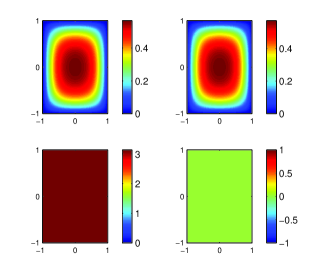
(a)  (b)

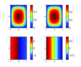
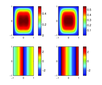
(c)  (d)

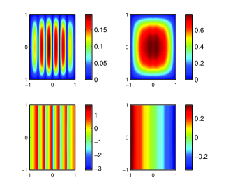
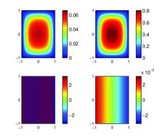
(e)  (f)

Fig. 1: Ground states $\tilde{\Phi}_{g}=(\tilde{\phi}_{1}^{g},\tilde{\phi}_{2}^{g})^{T}$ for a SO-coupled BEC in 2D with $\Omega=50$, $\delta=0$, $\beta_{11}=10$, $\beta_{12}=\beta_{21}=\beta_{22}=9$ for: (a) $k_{0}=0$, (b) $k_{0}=1$, (c) $k_{0}=5$, (d) $k_{0}=10$, (e) $k_{0}=50$, and (f) $k_{0}=100$. In each subplot, top panel shows densities and bottom panel shows phases of the ground state $\tilde{\phi}_{1}^{g}$ (left column) and $\tilde{\phi}_{2}^{g}$ (right column).

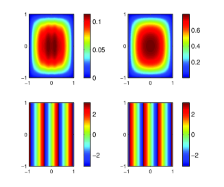
(a)  (b)

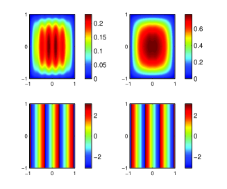
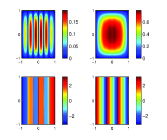
(c)  (d)

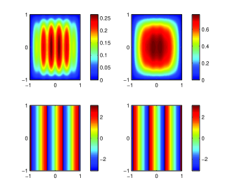
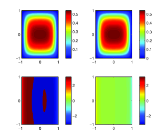
(e)  (f)

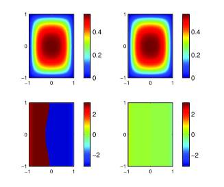
Fig. 2: Ground states $\Phi_{g}=(\phi_{1}^{g},\phi_{2}^{g})^{T}$ for a SO-coupled BEC in 2D with $k_{0}=10$, $\delta=0$, $\beta_{11}=10$, $\beta_{12}=\beta_{21}=\beta_{22}=9$ for: (a) $\Omega=1$, (b) $\Omega=10$, (c) $\Omega=50$, (d) $\Omega=200$, (e) $\Omega=300$, and (f) $\Omega=500$. In each subplot, top panel shows densities and bottom panel shows phases of the ground state $\phi_{1}^{g}$ (left column) and $\phi_{2}^{g}$ (right column).

Remark 3.1.

If the box potential

(44) $$V_{{\rm box}}({\bf x})=\begin{cases}0,&{\bf x}\in U,\\ +\infty,&\text{otherwise},\end{cases}$$

is used in the CGPEs (10) instead of the harmonic potentials (11), due to the appearance of the SO coupling, in order to compute the ground state, it is better to construct the GFDN based on (5) and then discretize it via the backward Euler sine pseudospectral (BESP) method due to that the homogeneous Dirichlet boundary condition on $\partial U$ must be used in this case. Again, for details, we refer to [5, 6, 7, 8] and references therein.

To test the efficiency and accuracy of the above numerical method for computing the ground state of SO-coupled BECs, we take $d=2$, $\delta=0$, $\beta_{11}:\beta_{12}:\beta_{22}=1:0.9:0.9$ with $\beta_{11}=10$ in (10). The potential $V_{j}({\bf x})$ ($j=1,2$) is taken as the box potential given in (44) with $U=[-1,1]\times[-1,1]$. We compute the ground state via the above BESP method with mesh size $h=\frac{1}{128}$ and time step $\tau=0.01$ ($\tau=0.001$ for large $\Omega$). For the chosen parameters, it is easy to find that when $\Omega=0$, the ground state $\Phi_{g}$ satisfies $\phi_{1}^{g}=0$ [4, 5]. Figure 1 shows the ground state $\tilde{\Phi}^{g}=(\tilde{\phi}_{1}^{g},\tilde{\phi}_{2}^{g})$ of (5) with $\Omega=50$ for different $k_{0}$, which clearly demonstrates that as $k_{0}\to\infty$, effect of $\Omega$ disappears. This is consistent with Theorem 3. Figure 2 depicts the ground state $\Phi^{g}$ with $k_{0}=10$ for different $\Omega$, from which we can observe that $\phi_{1}^{g}$ and $\phi_{2}^{g}$ tend to have the same density profile with opposite phase. This confirms Theorem 5.

3.2 For computing dynamics

In order to compute the dynamics of a SO-coupled BEC based on the CGPEs (10), we usually truncate it onto a bounded computational domain $U$, e.g. an interval $[a,b]$ in 1D, a rectangle $[a,b]\times[c,d]$ in 2D and a box $[a,b]\times[c,d]\times[e,f]$ in 3D, equipped with periodic boundary conditions. Then the CGPEs (10) can be solve via a time-splitting technique to decouple the nonlinearity [9, 4, 6, 2]. From $t_{n}$ to $t_{n+1}$, one first solves

(45) $$\begin{split}&i\partial_{t}\psi_{1}=\left(-\frac{1}{2}\Delta+ik_{0}\partial_{x}+\frac{\delta}{2}\right)\psi_{1}+\frac{\Omega}{2}\psi_{2},\\ &i\partial_{t}\psi_{2}=\left(-\frac{1}{2}\Delta-ik_{0}\partial_{x}-\frac{\delta}{2}\right)\psi_{2}+\frac{\Omega}{2}\psi_{1},\end{split}\qquad{\bf x}\in U,$$

for time $\tau$, followed by solving

(46) $$\begin{split}&i\partial_{t}\psi_{1}=\left(V_{1}({\bf x})+\beta_{11}|\psi_{1}|^{2}+\beta_{12}|\psi_{2}|^{2}\right)\psi_{1},\\ &i\partial_{t}\psi_{2}=\left(V_{2}({\bf x})+\beta_{21}|\psi_{1}|^{2}+\beta_{22}|\psi_{2}|^{2}\right)\psi_{2},\end{split}\qquad{\bf x}\in U,$$

for another time $\tau$. Eq. (45) with periodic boundary conditions can be discretized by the Fourier spectral method in space and then integrated in time exactly [9, 4, 6, 2]. Eq. (46) leaves the densities $|\psi_{1}|$ and $|\psi_{2}|$ unchanged and it can be integrated in time exactly [9, 4, 6, 2]. Then a full discretization scheme can be constructed via a combination of the splitting steps (45) and (46) with a second-order or higher-order time-splitting methods [9, 4, 6, 2].

For the convenience of the readers, here we present the method in 1D for the simplicity of notations. Extensions to 2D and 3D are straightforward. In 1D, let $h=\Delta x=(b-a)/N$ ($N$ an even positive integer), $x_{j}=a+jh$ ($j=0,\dotsc,N$), $\Psi_{j}^{n}=(\psi_{1,j}^{n},\psi_{2,j}^{n})^{T}$ be the numerical approximation of $\Psi(x_{j},t_{n})=(\psi_{1}(x_{j},t_{n}),\psi_{2}(x_{j},t_{n}))^{T}$, and for each fixed $l=1,2$, denote $\psi_{l}^{n}$ to be the vector consisting of $\psi_{l,j}^{n}$ for $j\in{\cal T}_{N}=\{0,1,\dotsc,N-1\}$. From time $t=t_{n}$ to $t=t_{n+1}$, a second-order time-splitting Fourier pseudospectral (TSFP) method for the CGPEs (10) in 1D reads [9, 6, 2]

(47) $$\begin{split}&\Psi^{(1)}_{j}=\frac{1}{N}\sum\limits_{k=-N/2}^{N/2-1}e^{i\mu_{k}(x_{j}-a)}\,Q_{k}^{T}\,e^{-\frac{i\tau}{4}U_{k}}\;Q_{k}(\widetilde{\Psi^{n}})_{k},\\ &\Psi_{j}^{(2)}=e^{-i\tau P_{j}^{(1)}}\;\Psi_{j}^{(1)},\qquad\qquad j=0,1,\dotsc,N-1,\\ &\Psi^{n+1}_{j}=\frac{1}{N}\sum\limits_{k=-N/2}^{N/2-1}e^{i\mu_{k}(x_{j}-a)}\,Q_{k}^{T}\,e^{-\frac{i\tau}{4}U_{k}}\;Q_{k}(\widetilde{\Psi^{(2)}})_{k},\end{split}$$

where for each fixed $k=-\frac{N}{2},-\frac{N}{2}+1,\dotsc,\frac{N}{2}-1$, $\mu_{k}=\frac{2k\pi}{b-a}$, $(\widetilde{\Psi}^{n})_{k}=((\widetilde{\psi_{1}^{n}})_{k},(\widetilde{\psi}_{2}^{n})_{k})^{T}$ with $(\widetilde{\psi_{l}^{n}})_{k}$ being the discrete Fourier transform coefficients of $\psi_{l}^{n}$ ($l=1,2$), $U_{k}=\text{diag}\left(\mu_{k}^{2}+2\lambda_{k},\mu_{k}^{2}-2\lambda_{k}\right)$ is a diagonal matrix, and

$$Q_{k}=\begin{pmatrix}\frac{\sqrt{\lambda_{k}-\chi_{k}}}{\sqrt{2\lambda_{k}}}&\frac{\frac{\Omega}{2}}{\sqrt{2\lambda_{k}(\lambda_{k}-\chi_{k})}}\\ \frac{-\sqrt{\lambda_{k}+\chi_{k}}}{\sqrt{2\lambda_{k}}}&\frac{\frac{\Omega}{2}}{\sqrt{2\lambda_{k}(\lambda_{k}+\chi_{k})}}\end{pmatrix}\quad\hbox{with}\quad\chi_{k}=k_{0}\mu_{k}-\frac{\delta}{2},\quad\lambda_{k}=\frac{1}{2}\sqrt{4\chi_{k}^{2}+\Omega^{2}},$$

and $P_{j}^{(1)}=\text{diag}\left(V_{1}(x_{j})+\sum\limits_{l=1}^{2}\beta_{1l}|\psi_{l,j}^{(1)}|^{2},V_{2}(x_{j})+\sum\limits_{l=1}^{2}\beta_{2l}|\psi_{l,j}^{(1)}|^{2}\right)$ for $j=0,1\dotsc,N-1$.

3.3 Box potential case

In some recent experiments of SO-coupled BEC, the box potential (44) is used. In this situation, due to that the homogeneous Dirichlet boundary condition on $\partial U$ must be used for the CGPEs (10), similarly to the computation of the ground states, it is better to adopt the CGPEs (16) for computing the dynamics. From $t=t_{n}$ to $t_{n+1}$, the CGPEs (16) will be split into the following three steps due to the appearance of the SO coupling. One first solves

(48) $$\begin{split}&i\partial_{t}\tilde{\psi}_{1}=\left(-\frac{1}{2}\Delta+\frac{\delta}{2}\right)\tilde{\psi}_{1},\\ &i\partial_{t}\tilde{\psi}_{2}=\left(-\frac{1}{2}\Delta-\frac{\delta}{2}\right)\tilde{\psi}_{2},\end{split}\qquad{\bf x}\in U,$$

for time step $\tau$, then solves

(49) $$\begin{split}&i\partial_{t}\tilde{\psi}_{1}=\left(V_{1}({\bf x})+\beta_{11}|\tilde{\psi}_{1}|^{2}+\beta_{12}|\tilde{\psi}_{2}|^{2}\right)\tilde{\psi}_{1},\\ &i\partial_{t}\tilde{\psi}_{2}=\left(V_{2}({\bf x})+\beta_{12}|\tilde{\psi}_{1}|^{2}+\beta_{22}|\tilde{\psi}_{2}|^{2}\right)\tilde{\psi}_{2},\end{split}\qquad{\bf x}\in U,$$

for time step $\tau$, followed by solving

(50) $$\begin{split}&i\partial_{t}\tilde{\psi}_{1}=\frac{\Omega}{2}e^{-i2k_{0}x}\tilde{\psi}_{2},\\ &i\partial_{t}\tilde{\psi}_{2}=\frac{\Omega}{2}e^{i2k_{0}x}\tilde{\psi}_{1},\end{split}\qquad{\bf x}\in U,$$

for time step $\tau$. Again, Eq. (48) with homogeneous Dirichlet boundary conditions can be discretized by the sine spectral method in space and then integrated in time exactly [9, 4, 6, 2]. Eq. (49) leaves the densities $|\tilde{\psi}_{1}|$ and $|\tilde{\psi}_{2}|$ unchanged and it can be integrated in time exactly [9, 4, 6, 2]. In addition, Eq. (50) is a linear ODE and can be integrated in time exactly as

(51) $$\tilde{\Psi}({\bf x},t_{n+1})=T(x)^{\ast}\,e^{-i\tau\Omega J}\,T(x)\,\tilde{\Psi}({\bf x},t_{n}),\ \hbox{with}\ T(x)=\frac{1}{\sqrt{2}}\begin{pmatrix}1&e^{-i2k_{0}x}\\ -1&e^{-i2k_{0}x}\end{pmatrix},$$

where $J=\text{diag}(-1,1)$ and $T(x)^{\ast}=\overline{T(x)}^{T}$ is the adjoint matrix of $T(x)$. Then a full discretization scheme can be constructed via a combination of the splitting steps (48)-(50) with a second-order method [9, 4, 6, 2]. The details are omitted here for brevity.

4 Dynamics of SO-coupled BEC

In this section, we study dynamical properties, in particular the motion of center-of-mass, of a SO-coupled BEC by using the CGPEs (10).

4.1 Dynamics of center-of-mass

Let $\Psi=(\psi_{1},\psi_{2})^{T}$ be the wave function describing the SO-coupled BEC, which is governed by the CGPEs (10). Define the center-of-mass of the BEC as

(52) $${\bf x}_{c}(t)=\int_{\mathbb{R}^{d}}{\bf x}\sum\limits_{j=1}^{2}|\psi_{j}({\bf x},t)|^{2}\,d{\bf x},\qquad t\geq 0,$$

and the momentum as

(53) $${{\bf P}}(t)=\int_{\mathbb{R}^{d}}\sum\limits_{j=1}^{2}\text{Im}(\overline{\psi_{j}({\bf x},t)}\nabla\psi_{j}({\bf x},t))\,d{\bf x},\qquad t\geq 0,$$

where $\text{Im}(f)$ denotes the imaginary part of the function $f$. In addition, we introduce the difference of the masses $N_{1}(t)$ and $N_{2}(t)$ in (14) of the two components in the SO-coupled BEC as

(54) $$\delta_{N}(t):=N_{1}(t)-N_{2}(t)=\int_{\mathbb{R}^{d}}\left[|\psi_{1}({\bf x},t)|^{2}-|\psi_{2}({\bf x},t)|^{2}\right]\,d{\bf x},\qquad t\geq 0.$$

Then the following lemma holds.

Lemma 10.

Let $V_{1}({\bf x})=V_{2}({\bf x})$ be the $d$-dimensional ($d=1,2,3$) harmonic potentials given in (11), then the motion of the center-of-mass ${\bf x}_{c}(t)$ for the CGPEs (10) is governed by

(55) $$\ddot{\bf x}_{c}(t)=-\Lambda{\bf x}_{c}(t)-2k_{0}\Omega\,\text{Im}\left(\int_{\mathbb{R}^{d}}\overline{\psi_{1}({\bf x},t)}\psi_{2}({\bf x},t)\,d{\bf x}\right)\,{\bf e}_{x},\qquad t>0,$$

where $\Lambda$ is a $d\times d$ diagonal matrix with $\Lambda=\gamma_{x}^{2}$ in 1D ($d=1$), $\Lambda=\text{diag}(\gamma_{x}^{2},\gamma_{y}^{2})$ in 2D ($d=2$) and $\Lambda=\text{diag}(\gamma_{x}^{2},\gamma_{y}^{2},\gamma_{z}^{2})$ in 3D ($d=3$), ${\bf e}_{x}$ is the unit vector for $x$-axis. The initial conditions for (55) are given as

$${\bf x}_{c}(0)=\int_{\mathbb{R}^{d}}{\bf x}\sum\limits_{j=1}^{2}|\psi_{j}({\bf x},0)|^{2}\,d{\bf x},\qquad\dot{{\bf x}}_{c}(0)={\bf P}(0)-k_{0}\delta_{N}(0)\,{\bf e}_{x}.$$

In particular, (55) implies that the center-of-mass ${\bf x}_{c}(t)$ is periodic in $y$-component with frequency $\gamma_{y}$ when $d=2,3$, and in $z$-component with frequency $\gamma_{z}$ when $d=3$. If $k_{0}\Omega=0$, ${\bf x}_{c}(t)$ is also periodic in $x$-component with frequency $\gamma_{x}$.

Proof.

For $j=1,2$, differentiating ${\bf x}_{j}(t)=\int_{\mathbb{R}^{d}}{\bf x}|\psi_{j}({\bf x},t)|^{2}\,d{\bf x}$, using the CGPEs (10) and integral by parts, we find

$$\dot{\bf x}_{j}(t)={\bf P}_{j}(t)-k_{0}(3-2j)N_{j}(t)\,{\bf e}_{x}-\frac{i\Omega}{2}\int_{\mathbb{R}^{d}}{\bf x}\left(\overline{\psi}_{j}\psi_{3-j}-\psi_{j}\overline{\psi}_{3-j}\right)\,d{\bf x},$$

where ${\bf P}_{j}(t):=\int_{\mathbb{R}^{d}}\text{Im}(\overline{\psi_{j}({\bf x},t)}\nabla\psi_{j}({\bf x},t))\,d{\bf x}$. Summing the above equation for $j=1,2$ and noticing (52) and (53), we get

(56) $$\dot{\bf x}_{c}(t)={\bf P}(t)-k_{0}\delta_{N}(t)\,{\bf e}_{x},\qquad t\geq 0.$$

Differentiating (56) once more, we get

(57) $$\ddot{\bf x}_{c}(t)=\dot{\bf P}(t)-k_{0}\dot{\delta}_{N}(t)\,{\bf e}_{x}.$$

We now compute the RHS of (57). Firstly, for $j=1,2$, differentiating ${\bf P}_{j}(t)$, making use of the CGPEs (10) and integral by parts, we get

$$\dot{\bf P}_{j}(t)=\int_{\mathbb{R}^{d}}\left[-|\psi_{j}|^{2}\nabla V_{j}({\bf x})-\beta_{12}|\psi_{3-j}|^{2}\nabla|\psi_{j}|^{2}+\Omega\,\text{Re}(\overline{\psi}_{3-j}\nabla\psi_{j})\right]\,d{\bf x},$$

which immediately gives

(58) $$\dot{\bf P}(t)=-\int_{\mathbb{R}^{d}}\Lambda{\bf x}\sum\limits_{j=1}^{2}|\psi_{j}|^{2}\,d{\bf x}=-\Lambda{\bf x}_{c}(t),$$

with $\Lambda$ being the diagonal matrix described in the lemma. Secondly, for $j=1,2$, differentiating $N_{j}(t)$, making use of the CGPEs (10) and integral by parts, we obtain

$$\dot{N}_{j}(t)=-\frac{i\Omega}{2}\int_{\mathbb{R}^{d}}\left(\overline{\psi}_{j}\psi_{3-j}-\overline{\psi}_{3-j}\psi_{j}\right)\,d{\bf x},$$

which again immediately implies

(59) $$\dot{\delta}_{N}(t)=2\Omega\,\text{Im}\int_{\mathbb{R}^{d}}\overline{\psi_{1}({\bf x},t)}\psi_{2}({\bf x},t)\,d{\bf x}.$$

Combining (59), (58) and (57), we draw the conclusion. ∎

From Lemma 10, the effect of SO coupling on the motion of the center-of-mass ${\bf x}_{c}(t)$ appears in the $x$-component. Denote the $x$-component of ${\bf x}_{c}(t)$ as $x_{c}(t)$, and the $x$-component of ${\bf P}(t)$ as $P^{x}(t)$. Then we have the following results:

Theorem 11.

Let $V_{1}({\bf x})=V_{2}({\bf x})$ be the harmonic potential as (11) in $d$ dimensions ($d=1,2,3$) and $k_{0}\Omega\neq 0$. For the $x$-component $x_{c}(t)$ of the center-of-mass ${\bf x}_{c}(t)$ of the CGPEs (10) with any initial data $\Psi({\bf x},0):=\Psi_{0}({\bf x})$ satisfying $\|\Psi_{0}\|=1$, we have

(60) $$x_{c}(t)=x_{0}\cos(\gamma_{x}t)+\frac{P_{0}^{x}}{\gamma_{x}}\sin(\gamma_{x}t)-k_{0}\int_{0}^{t}\cos(\gamma_{x}(t-s))\delta_{N}(s)\,ds,\qquad t\geq 0,$$

where $x_{0}=\int_{\mathbb{R}^{d}}x\sum_{j=1}^{2}|\psi_{j}({\bf x},0)|^{2}\,d{\bf x}$ and $P_{0}^{x}=\int_{\mathbb{R}^{d}}\sum_{j=1}^{2}\text{Im}(\overline{\psi_{j}({\bf x},0)}\partial_{x}\psi_{j}({\bf x},0))\,d{\bf x}$. In addition, if $\delta=0$, $\beta_{11}=\beta_{12}=\beta_{22}$ and $|k_{0}|$ is small, we can approximate the solution $x_{c}(t)$ as follows:

(i) If $|\Omega|=\gamma_{x}$, we can get

$$x_{c}(t)\approx\left(x_{0}-\frac{k_{0}}{2}\delta_{N}(0)t\right)\cos(\gamma_{x}t)+\frac{1}{\gamma_{x}}\left(P_{0}^{x}-\frac{k_{0}}{2}\delta_{N}(0)-{\rm sgn}(\Omega)\frac{\gamma_{x}k_{0}C_{0}}{2}t\right)\sin(\gamma_{x}t),$$

where $C_{0}=2\text{Im}\int_{\mathbb{R}^{d}}\overline{\psi_{1}({\bf x},0)}\psi_{2}({\bf x},0)\,d{\bf x}$.

(ii) If $|\Omega|\neq\gamma_{x}$, we can get

$$\begin{split}x_{c}(t)\approx&\left(x_{0}+\frac{k_{0}C_{0}}{\gamma_{x}^{2}-\Omega^{2}}\right)\cos(\gamma_{x}t)+\frac{1}{\gamma_{x}}\left(P_{0}^{x}-\frac{\gamma_{x}^{2}k_{0}\delta_{N}(0)}{\gamma_{x}^{2}-\Omega^{2}}\right)\sin(\gamma_{x}t)\\ &-\frac{k_{0}C_{0}}{\gamma_{x}^{2}-\Omega^{2}}\cos(\Omega t)+\frac{k_{0}\delta_{N}(0)\Omega}{\gamma_{x}^{2}-\Omega^{2}}\sin(\Omega t).\end{split}$$

Based on the above approximation, if $|\Omega|=\gamma_{x}$ or $\frac{\Omega}{\gamma_{x}}$ is an irrational number, $x_{c}(t)$ is not periodic; and if $\frac{\Omega}{\gamma_{x}}$ is a rational number, $x_{c}(t)$ is a periodic function, but its frequency is different from the trapping frequency $\gamma_{x}$.

Proof.

Solving (55) by the variation-of-constant formula and using (59), we have

$$x_{c}(t)=x_{c}(0)\cos(\gamma_{x}t)+\frac{P^{x}(0)-k_{0}\delta_{N}(0)}{\gamma_{x}}\sin(\gamma_{x}t)-\frac{k_{0}}{\gamma_{x}}\int_{0}^{t}\cos(\gamma_{x}(t-s))\dot{\delta}_{N}(s)\,ds,$$

and (60) follows by applying integration by parts.

In order to obtain the prescribed approximation, we first find the equation for $\delta_{N}(t)$. Differentiating (59) and using (10), we get

$$\ddot{\delta}_{N}(t) =-\Omega^{2}\delta_{N}(t)+2\Omega\,\text{Re}\int_{\mathbb{R}^{d}}\bigg{[}\big{(}V_{1}({\bf x})-V_{2}({\bf x})+\delta+(\beta_{11}-\beta_{21})|\psi_{1}|^{2}$$

$$\qquad\qquad\qquad+(\beta_{12}-\beta_{22})|\psi_{2}|^{2}\big{)}\overline{\psi_{1}}\psi_{2}+ik_{0}(\overline{\psi}_{1}\partial_{x}\psi_{2}-\overline{\partial_{x}\psi_{1}}\psi_{2})\bigg{]}\,d{\bf x}.$$

Thus, if $|k_{0}|\ll 1$ and $\delta=0$, $\beta_{11}=\beta_{12}=\beta_{22}$, the above equation is approximated by

(61) $$\ddot{\delta}_{N}(t)\approx-\Omega^{2}N_{\Delta}(t),$$

and the initial condition $\dot{\delta}_{N}(0)$ can be obtained via (59) with $t=0$. Solving the above ODE, we find

(62) $$\delta_{N}(t)\approx\delta_{N}(0)\cos(\Omega t)+\frac{\dot{\delta}_{N}(0)}{\Omega}\sin(\Omega t).$$

Plugging (62) into (60), we obtain the approximate solution of $x_{c}(t)$. ∎

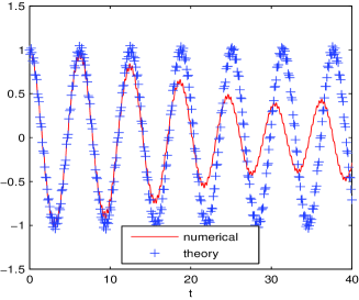
(a)  (b)

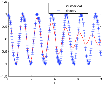
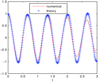
(c)  (d)

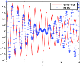
Fig. 3: Time evolution of the center-of-mass $x_{c}(t)$ for the CGPEs (10) obtained numerically from its numerical solution (i.e. labeled as ’numerical’ with solid lines) and asymptotically as in Theorem 11 (i.e. labeled as ’theory’ with ‘+ + +’) with $\Omega=20$ and $k_{0}=1$ for different $\gamma_{x}$: (a) $\gamma_{x}=1$, (b) $\gamma_{x}=5$, (c) $\gamma_{x}=3\pi$, and (d) $\gamma_{x}=20$.

To verify the asymptotic (or approximate) results for $x_{c}(t)$ in Theorem 11, we numerically solve the CGPEs (10) with (11) in 2D (i.e. $d=2$), take $\beta_{11}=\beta_{12}=\beta_{22}=10$, $\delta=0$ and choose the initial data as

(63) $$\psi_{1}({\bf x},0)=\pi^{-1/2}e^{-\frac{|{\bf x}-{\bf x}_{0}|^{2}}{2}},\quad\psi_{2}({\bf x},0)=0,\quad{\bf x}\in{\mathbb{R}}^{2},$$

where ${\bf x}_{0}=(1,1)^{T}$. Figure 3 depicts time evolution of $x_{c}(t)$ obtained numerically and asymptotically as in Theorem 11 with $\Omega=20$ and $k_{0}=1$ for different $\gamma_{x}$. From this figure, we see that: for short time $t$, the approximation given in Theorem 11 is very accurate; and when $t\gg 1$, it becomes inaccurate, which is due to that the assumption on $\delta_{N}(t)$ obeying (62) becomes inaccurate.

In fact, Theorem 11 is valid for any given initial data. Now, we consider a kind of special initial data, i.e. shift of the ground state $\Phi_{g}=(\phi_{1}^{g},\phi_{2}^{g})^{T}$ of (1) for the CGPEs (10), i.e., the initial condition for (10) is chosen as

(64) $$\psi_{1}({\bf x},0)=\phi_{1}^{g}({\bf x}-{\bf x}_{0}),\quad\psi_{2}({\bf x},0)=\phi_{2}^{g}({\bf x}-{\bf x}_{0}),\qquad{\bf x}\in{\mathbb{R}}^{d},$$

where ${\bf x}_{0}=x_{0}$ in 1D, ${\bf x}_{0}=(x_{0},y_{0})^{T}$ in 2D and ${\bf x}_{0}=(x_{0},y_{0},z_{0})^{T}$ in 3D. Then we have the approximate dynamical law for the center-of-mass in $x$-direction $x_{c}(t)$.

Theorem 12.

Suppose $V_{1}({\bf x})=V_{2}({\bf x})$ for ${\bf x}\in{\mathbb{R}}^{d}$ are harmonic potentials given in (11), $\beta_{11}=\beta_{12}=\beta_{22}=\beta$ and the initial data for the CGPEs (10) is taken as (64). Using the local density approximation (LDA), the dynamics of the center-of-mass $x_{c}(t)$ can be approximated by the following ODE

(65) $$\dot{x}_{c}(t)=P^{x}(t)-\frac{k_{0}[2k_{0}P^{x}(t)-\delta]}{\sqrt{[2k_{0}P^{x}(t)-\delta]^{2}+\Omega^{2}}},\quad\dot{P}^{x}(t)=-\gamma_{x}^{2}x_{c}(t),\qquad t\geq 0,$$

with $x_{c}(0)=x_{0}$ and $P^{x}(0)=k_{0}\delta_{N}(0)$. In particular, the solution to (65) is periodic, and, in general, its frequency is different with the trapping frequency $\gamma_{x}$.

Proof.

The initial condition for the ODE (65) comes from the initial value (64) for the CGPEs (10). We use LDA here, which means we will treat the BEC system as a uniform system $V_{1}({\bf x})=V_{2}({\bf x})=\text{constant}$ locally. We begin with the uniform case. The evolution of the wave function $\Psi=(\psi_{1},\psi_{2})^{T}$ is assumed to remain in the ground mode of the Hamiltonian

(66) $${\bf H}=\begin{pmatrix}-\frac{\nabla^{2}}{2}+ik_{0}\partial_{x}+\frac{\delta}{2}+\beta|\Psi|^{2}&\frac{\Omega}{2}\\ \frac{\Omega}{2}&-\frac{\nabla^{2}}{2}-ik_{0}\partial_{x}-\frac{\delta}{2}+\beta|\Psi|^{2}\end{pmatrix},$$

and be localized near the center-of-mass ${\bf x}_{c}(t)$ in physical space and near the momentum ${\bf P}(t)$ in the phase space. Thus, the wave function can be written as

(67) $$\Psi=(\psi_{1},\psi_{2})^{T}=e^{i{\xi\cdot({\bf x}-{\bf x}_{c}(t))}}\vec{v},\quad\vec{v}\quad\text{is a vector in}\quad\mathbb{C}^{2},$$

and $\xi=(\xi_{1},\dotsc,\xi_{d})^{T}\in\mathbb{R}^{d}$ is centered around ${\bf P}(t)$. Plugging (67) into (66), we obtain a two-by-two matrix, and the two eigenvalues and the corresponding eigenvectors are

(68) $${\cal E}_{\pm}=\frac{|\xi|^{2}}{2}+\beta|\vec{v}|^{2}\pm\tilde{\lambda},\quad\vec{v}_{\pm}=\left(\frac{(\tilde{\lambda}\mp\tilde{\chi})^{1/2}}{(2\tilde{\lambda})^{1/2}},\frac{\Omega}{2(2\tilde{\lambda}(\tilde{\lambda}\mp\tilde{\chi}))^{1/2}}\right)^{T},$$

with $\tilde{\lambda}=\frac{1}{2}\sqrt{(2k_{0}\xi_{1}-\delta)^{2}+\Omega^{2}}$ and $\tilde{\chi}=k_{0}\xi_{1}-\frac{\delta}{2}$. By our assumption that the evolution is in the lower eigenstate, we find $\vec{v}=|\vec{v}|\vec{v}_{-}$ and

(69) $$\frac{|\psi_{1}|^{2}}{|\psi_{2}|^{2}}=\frac{4(\tilde{\lambda}+\tilde{\chi})^{2}}{\Omega^{2}}.$$

Since the phase space is assumed to be localized around ${\bf P}(t)$, we can approximate the above equation by letting $\xi_{1}=P^{x}:=P^{x}(t)$ and we get

(70) $$\frac{|\psi_{1}|^{2}}{|\psi_{2}|^{2}}\approx\frac{4(\lambda+\chi)^{2}}{\Omega^{2}},\quad\lambda=\frac{1}{2}\sqrt{(2k_{0}P^{x}-\delta)^{2}+\Omega^{2}},\quad\chi=k_{0}P^{x}-\frac{\delta}{2}.$$

For the case with harmonic potentials $V_{1}({\bf x})=V_{2}({\bf x})$, we use LDA, and we could get the same relation between densities as (70) for each position ${\bf x}$ which leads to

(71) $$\delta_{N}(t)=\frac{4(\lambda+\chi)^{2}-\Omega^{2}}{4(\lambda+\chi)^{2}+\Omega^{2}}.$$

Plugging (71) into (56), noticing (58), we obtain the ODE system (65) approximating the dynamics of $x_{c}(t)$. Using the equation (65), it is easy to find that

(72) $$\frac{d}{dt}\left(\gamma_{x}^{2}x_{c}^{2}(t)+(P^{x}(t))^{2}-\sqrt{[2k_{0}P^{x}(t)-\delta]^{2}+\Omega^{2}}\right)=0,$$

which shows $(x_{c}(t),P^{x}(t))^{T}$ is a closed curve and it is periodic. ∎

Again, to verify the asymptotic (or approximate) results for $x_{c}(t)$ in Theorem 12, we numerically solve the CGPEs (10) with (11) in 2D (i.e. $d=2$), take $\beta_{11}=\beta_{12}=\beta_{22}=10$ and $\gamma_{x}=\gamma_{y}=2$, and choose the initial data as (64) with ${\bf x}_{0}=(2,2)^{T}$ and the ground state computed numerically. Figure 4 depicts time evolution of $x_{c}(t)$ obtained numerically and asymptotically as in Theorem 12 with different $\Omega$, $k_{0}$ and $\delta$.

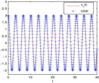
(a)  (b)

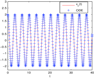
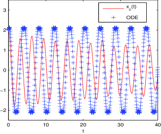
(c)  (d)

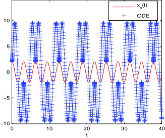
Fig. 4: Time evolution of the center-of-mass $x_{c}(t)$ for the CGPEs (10) obtained numerically from its numerical solution (i.e. labeled as $x_{c}(t)$ with solid lines) and asymptotically as in Theorem 12 (i.e. labeled as ’ODE’ with ‘+ + +’) for different sets of parameters: (a) $(\Omega,k_{0},\delta)=(50,2,0)$, (b) $(\Omega,k_{0},\delta)=(50,2,10)$, (c) $(\Omega,k_{0},\delta)=(2,2,0)$, and (d) $(\Omega,k_{0},\delta)=(50,20,0)$.

From Figure 4 and numerous tests we have done (not shown here for brevity), we find that for the very special initial data (64), Theorem 12 provides a very good approximation for the dynamics of the center-of-mass over a long time when $|\Omega|$ is much larger than $\gamma_{x}$ and $k_{0}$. However, when $0<\gamma_{x}\ll|\Omega|$ and $k_{0}$ is large, $x_{c}(t)$ behaves periodically over a long time, but the approximation in Theorem 12 fails! For $|\Omega|$ being comparable to $\gamma_{x}$, $x_{c}(t)$ is damped in time and non-periodic.

Remark 4.1.

Theorem 12 does not contradict with Theorem 11, because Theorem 11 holds for small $k_{0}$, where the $\Omega$ frequency contribution is very small and $x_{c}(t)$ is almost periodic there. Theorem 12 has certain restriction because of the assumptions we have used on the initial data. In particular, $k_{0}$ can not be large because the energy gap between ground modes and excited modes will be reduced for large $k_{0}$ and the assumption that the wave function remains in the ground mode will be violated.

4.2 Semi-classical scaling

For strong interaction $\beta_{jl}\gg 1$, we could rescale (10) by choosing ${\bf x}\to{\bf x}\varepsilon^{-1/2}$ , $\psi_{j}\to\psi^{\varepsilon}_{j}\varepsilon^{d/4}$, $\varepsilon=1/\beta^{2/(d+2)}$, $\beta=\max\{|\beta_{11}|,|\beta_{12}|,|\beta_{22}|\}$, which gives the following CGPEs

(73) $$\begin{split}&i\varepsilon\partial_{t}\psi_{1}^{\varepsilon}=\left[-\frac{\varepsilon^{2}}{2}\nabla^{2}+V_{1}({\bf x})+ik_{0}\varepsilon^{3/2}\partial_{x}+\frac{\delta\varepsilon}{2}+\sum_{j=1}^{2}\beta_{1j}^{0}|\psi^{\varepsilon}_{j}|^{2}\right]\psi^{\varepsilon}_{1}+\frac{\Omega\varepsilon}{2}\psi^{\varepsilon}_{2},\\ &i\varepsilon\partial_{t}\psi^{\varepsilon}_{2}=\left[-\frac{\varepsilon^{2}}{2}\nabla^{2}+V_{2}({\bf x})-ik_{0}\varepsilon^{3/2}\partial_{x}-\frac{\delta\varepsilon}{2}+\sum_{j=1}^{2}\beta_{2j}^{0}|\psi^{\varepsilon}_{j}|^{2}\right]\psi^{\varepsilon}_{2}+\frac{\Omega\varepsilon}{2}\psi^{\varepsilon}_{1},\end{split}$$

where $\beta_{j,l}^{0}=\frac{\beta_{j,l}}{\beta}$ and the potential functions are given in (11). It is of great interest to study the behavior of (73) when the small parameter $\varepsilon$ tends to 0.

Semiclassical limits in linear case. In the linear case, i.e. $\beta_{jl}^{0}=0$ for $j,l=1,2$, (73) collapses to

(74) $$i\varepsilon\partial_{t}\Psi^{\varepsilon}=\begin{bmatrix}\frac{-\varepsilon^{2}}{2}\Delta+ik_{0}\varepsilon^{3/2}\partial_{x}+\frac{\delta\varepsilon}{2}+V_{1}&\frac{\Omega\varepsilon}{2}\\ \frac{\Omega\varepsilon}{2}&\frac{-\varepsilon^{2}}{2}\Delta-ik_{0}\varepsilon^{3/2}\partial_{x}-\frac{\delta\varepsilon}{2}+V_{2}\end{bmatrix}\Psi^{\varepsilon}$$

where $\Psi^{\varepsilon}=(\psi_{1}^{\varepsilon},\psi_{2}^{\varepsilon})^{T}$. We now describe the limit as $\varepsilon\to 0^{+}$ using the Wigner transform

(75) $$W^{\varepsilon}(\Psi^{\varepsilon})({\bf x},\xi)=(2\pi)^{-d}\int_{\mathbb{R}^{d}}\Psi^{\varepsilon}({\bf x}-\varepsilon v/2)\otimes\Psi^{\varepsilon}({\bf x}+\varepsilon v/2)e^{iv\cdot\xi}\,dv,$$

where $W^{\varepsilon}$ is a $2\times 2$ matrix-valued function. The symbol corresponds to (74) can be written as

(76) $$P^{\varepsilon}({\bf x},\xi)=\frac{i}{2}|\xi|^{2}+i\begin{bmatrix}k_{0}\varepsilon^{1/2}\xi_{1}+V_{1}({\bf x})+\frac{\delta\varepsilon}{2}&\frac{\Omega\varepsilon}{2}\\ \frac{\Omega\varepsilon}{2}&-k_{0}\varepsilon^{1/2}\xi_{1}+V_{2}({\bf x})-\frac{\delta\varepsilon}{2}\end{bmatrix},$$

where $\xi=(\xi_{1},\xi_{2},\dotsc,\xi_{d})^{T}$. Let us consider the principal part $P$ of $P^{\varepsilon}=P+O(\varepsilon)$, i.e., we omit small term $O(\varepsilon)$, and we know that $-iP({\bf x},\xi)$ has two eigenvalues $\lambda_{1}({\bf x},\xi)$ and $\lambda_{2}({\bf x},\xi)$. Let $\Pi_{j}$ ($j=1,2$) be the projection matrix from $\mathbb{C}^{2}$ to the eigenvector space associated with $\lambda_{j}$. If $\lambda_{1,2}$ are well separated, then $W^{\varepsilon}(\Psi^{\varepsilon})$ converges to the Wigner measure $W^{0}$ which can be decomposed as [15]

(77) $$W^{0}=u_{1}({\bf x},\xi,t)\Pi_{1}+u_{2}({\bf x},\xi,t)\Pi_{2},$$

where $u_{j}({\bf x},\xi,t)$ satisfies the Liouville equation

(78) $$\partial_{t}u_{j}({\bf x},\xi,t)+\nabla_{\xi}\lambda_{j}({\bf x},\xi,t)\cdot\nabla_{{\bf x}}u_{j}({\bf x},\xi,t)-\nabla_{{\bf x}}\lambda_{j}({\bf x},\xi,t)\cdot\nabla_{\xi}u_{j}({\bf x},\xi,t)=0.$$

It is known that such semi-classical limit fails at regions when $\lambda_{1}$ and $\lambda_{2}$ are close.

Specifically, when $k_{0}=O(1)$, $\delta=O(1)$ and $\Omega=O(1)$, the limit of the Wigner transform $W^{\varepsilon}(\Psi^{\varepsilon})$ only has diagonal elements, and we have

(79) $$P=\frac{i}{2}|\xi|^{2}+i\begin{bmatrix}V_{1}({\bf x})&0\\ 0&V_{2}({\bf x})\end{bmatrix},\quad\lambda_{1}=\frac{1}{2}|\xi|^{2}+V_{1}({\bf x}),\quad\lambda_{2}=\frac{1}{2}|\xi|^{2}+V_{2}({\bf x}).$$

In the limit of this case, $W^{0}$ in (77), $\Pi_{1}$ and $\Pi_{2}$ are diagonal matrices, which means the two components of $\Psi^{\varepsilon}$ in (74) are decoupled as $\varepsilon\to 0^{+}$. In addition, the Liouville equation (78) is valid with $\lambda_{1}$ and $\lambda_{2}$ defined in (79).

Similarly, when $k_{0}=O(1/\varepsilon^{1/2})$, $\delta=O(1/\varepsilon)$ and $\Omega=O(1/\varepsilon)$, e.g. $k_{0}=\frac{k_{\infty}}{\varepsilon^{1/2}}$, $\Omega=\frac{\Omega_{\infty}}{\varepsilon}$ and $\delta=\frac{\delta_{\infty}}{\varepsilon}$ with $k_{\infty}$, $\Omega_{\infty}$ and $\delta_{\infty}$ nonzero constants, the limit of the Wigner transform $W^{\varepsilon}(\Psi^{\varepsilon})$ has nonzero diagonal and off-diagonal elements, and we have

(80) $$P=\frac{i}{2}|\xi|^{2}+i\begin{bmatrix}k_{\infty}\xi_{1}+V_{1}({\bf x})+\frac{\delta_{\infty}}{2}&\frac{\Omega_{\infty}}{2}\\ \frac{\Omega_{\infty}}{2}&-k_{\infty}\xi_{1}+V_{2}({\bf x})-\frac{\delta_{\infty}}{2}\end{bmatrix},$$

and

(81) $$\lambda_{1,2}=\frac{|\xi|^{2}}{2}+\frac{V_{1}({\bf x})+V_{2}({\bf x})}{2}\pm\frac{\sqrt{[V_{1}({\bf x})-V_{2}({\bf x})+2k_{\infty}\xi_{1}+\delta_{\infty}]^{2}+\Omega_{\infty}^{2}}}{2}.$$

In the limit of this case, $W^{0}$ in (77), $\Pi_{1}$ and $\Pi_{2}$ are full matrices, which means that the two components of $\Psi^{\varepsilon}$ in (74) are coupled as $\varepsilon\to 0^{+}$. Again, the Liouville equation (78) is valid with $\lambda_{1}$ and $\lambda_{2}$ defined in (81).

Of course, for the nonlinear case, i.e. $\beta_{jl}^{0}\neq 0$ for $j,l=1,2$, only the case when $\Omega=0$ and $k_{0}=0$ has been addressed [19]. For $\Omega\neq 0$ and $k_{0}\neq 0$, it is still not clear about the semi-classical limit of the CGPEs (73).

5 Conclusions

We have studied analytically and asymptotically as well as numerically ground states and dynamics of two-component spin-orbit-coupled Bose-Einstein condensates (BECs) based on the coupled Gross-Pitaevskii equations (CGPEs) with the spin-orbit (SO) and Raman couplings. For ground state properties, we established existence and uniqueness, as well as non-existence of the grounds states in different parameter regimes and studied their limiting behavior and structure with various combination of the SO and Raman coupling strengths. Efficient and accurate numerical methods were designed for computing the ground states and dynamics of SO-coupled BECs, especially for box potentials. Numerical results for the ground states were reported under different parameter regimes, which confirmed our analytical results on ground states. For dynamical properties, we obtained the dynamical laws governing the motion of the center-of-mass and showed that the dynamics of the center-of-mass in the SO-coupled direction is either non-periodic or a periodic function with different frequency to the trapping frequency, which is completely different from the case without SO coupling. Numerical results were presented to confirm our asymptotical (or approximate) results on the dynamics of the center-of-mass. Finally, we described the semi-classical limit of the CGPEs in the linear case via the Wigner transform method.

References

- [1] M. H. Anderson, J. R. Ensher, M. R. Matthewa, C. E. Wieman and E. A. Cornell, Observation of Bose-Einstein condensation in a dilute atomic vapor, Science, 269 (1995), pp. 198–201.
- [2] X. Antoine, W. Bao and C. Besse, Computational methods for the dynamics of the nonlinear Schrödinger/Gross-Pitaevskii equations, Comput. Phys. Commun., 184 (2013), pp. 2621-2633.
- [3] W. Bao, Mathematical models and numerical methods for Bose-Einstein condensation, Proceeding of International Congress of Mathematicians, 2014, to appear (arXiv: 1403.3884 (math.ph)).
- [4] W. Bao, Ground states and dynamics of multicomponent Bose–Einstein condensates, Multiscale Model. Simul., 2 (2004), pp. 210–236.
- [5] W. Bao and Y. Cai, Ground states of two-component Bose-Einstein condensates with an internal atomic Josephson junction, East Asia J. Appl. Math., 1 (2010), pp. 49–81.
- [6] W. Bao and Y. Cai, Mathematical theory and numerical methods for Bose-Einstein condensation, Kinet. Relat. Mod., 6 (2013), pp. 1–135.
- [7] W. Bao, I-L. Chern and F. Y. Lim, Efficient and spectrally accurate numerical methods for computing ground and first excited states in Bose-Einstein condensates, J. Comput. Phys., 219 (2006), pp. 836-854.
- [8] W. Bao and Q. Du, Computing the ground state solution of Bose-Einstein condensates by a normalized gradient flow, SIAM J. Sci. Comput., 25 (2004), pp. 1674-1697.
- [9] W. Bao, D. Jaksch and P. A. Markowich, Numerical solution of the Gross-Pitaevskii equation for Bose-Einstein condensation, J. Comput. Phys., 187 (2003), pp. 318 - 342.
- [10] N. Ben Abdallah, F. Méhats, C. Schmeiser and R. M. Weishäupl The nonlinear Schrödinger equation with a strongly anisotropic harmonic potential, SIAM J. Math. Anal., 47 (2005), pp. 189–199.
- [11] S. M. Chang, C. S. Lin, T. C. Lin and W. W. Lin, Segregated nodal domains of two-dimensional multispecies Bose-Einstein condensates, Physica D, 196 (2004), pp. 341-361.
- [12] K. B. Davis, M. O. Mewes, M. R. Andrews, N. J. van Druten, D. S. Durfee, D. M. Kurn and W. Ketterle, Bose-Einstein condensation in a gas of sodium atoms, Phys. Rev. Lett., 75 (1995), pp. 3969–3973.
- [13] Y. Deng, J. Cheng, H. Jing, C. P. Sun and S. Yi, Spin-orbit-coupled dipolar Bose-Einstein condensates, Phys. Rev. Lett., 108 (2012), 125301.
- [14] V. Galitski and I. B. Spielman, Spin-orbit coupling in quantum gases, Nature, 494 (2012), pp. 49-54.
- [15] P. Gérard, P. A. Markowich and NJ Mauser, Homogenization limits and Wigner transforms, Comm. Pure Appl. Math., 50 (1997), 323–379.
- [16] C. Hamner, Y. Zhang, M. A. Khamehchi, M. J. Davis and P. Engels, Spin-orbit coupled Bose-Einstein condensates in a one-dimensional optical lattice, arXiv:1405.4048.
- [17] M. Z. Hasan and C. L. Kane, Colloquium: Topological insulators, Rev. Mod. Phys., 82 (2010), 3045–3067.
- [18] H. Hu, B. Ramachandhran, H. Pu and X. Liu, Spin-orbit coupled weakly interacting Bose-Einstein condensates in harmonic traps, Phys. Rev. Lett., 108 (2012), 010402.
- [19] C.-C. Lee and T.-C. Lin, Incompressible and compressible limits of two-component Gross CPitaevskii equations with rotating fields and trap potentials, J. Math. Phys., 49 (2008), 043517.
- [20] Y. Li, L. Pitaevskii and S. Stringari, Quantum tricriticality and phase transitions in spin-orbit coupled Bose-Einstein condensates, Phys. Rev. Lett., 108 (2012), article 225301.
- [21] Y. Li, G. I. Martone, L. Pitaevskii and S. Stringari, Superstripes and the excitation spectrum of a spin-orbit-coupled Bose-Einstein condensate, Phys. Rev. Lett., 110 (2013), article 235302.
- [22] E. H. Lieb and M. Loss, Analysis, Graduate Studies in Mathematics, Amer. Math. Soc., 2nd ed., 2001.
- [23] E. H. Lieb, R. Seiringer and J. Yngvason, Bosons in a trap: a rigorous derivation of the Gross-Pitaevskii energy functional, Phy. Rev. A, 61 (2000), article 043602.
- [24] E. H. Lieb and J. P. Solovej, Ground state energy of the two-component charged Bose gas, Comm. Math. Phys., 252 (2004), pp. 485-534.
- [25] Y. J. Lin, K. Jiménez-Garcia and I. B. Spielman, Spin-orbit-coupled Bose-Einstein condensates, Nature, 471 (2011), 83–86.
- [26] Z. Liu, Two-component Bose-Einstein condensates, J. Math. Anal. Appl., 348 (2008), pp. 274-285.
- [27] L. P. Pitaevskii and S. Stringari, Bose-Einstein Condensation, Clarendon Press, Oxford, 2003.
- [28] C. Wang, C. Gao, C. Jian and H. Zhai, Spin-orbit coupled spinor Bose-Einstein condensates, Phys. Rev. Lett., 105 (2010), 160403.
- [29] H. Wang and Z. Xu, A projection gradient method for energy functional minimization with a constraint and its application into computing ground state of spin-orbit-coupled Bose-Einstein condensate, Comp. Phys. Comm., in press.
- [30] M. I. Weinstein, Nonlinear Schrödinger equations and sharp interpolation estimates, Comm. Math. Phys., 87 (1983), pp. 567-576.
- [31] D. Xiao, M. Chang and Q. Niu, Berry phase effects on electronic properties, Rev. Mod. Phys., 82 (2010), pp. 1959–2007.
- [32] J. Zhang, S. Ji, Z. Chen, L. Zhang, Z. Du, B. Yan, G. Pan, B. Zhao, Y. Deng, H. Zhai, S. Chen and J. Pan Collective dipole oscillations of a spin-orbit coupled Bose-Einstein condensate, Phys. Rev. Lett., 109 (2012), 115301.
- [33] Y. Zhang, L. Mao and C. Zhang, Mean-field dynamics of spin-orbit coupled Bose-Einstein condensates, Phys. Rev. Lett., 108 (2012), 035302.
- [34] Q. Zhu, C. Zhang and B. Wu, Exotic superfluidity in spin-orbit coupled Bose-Einstein condensates, Europhys. Lett., 100 (2012), 50003.