State-dependent photon blockade via quantum-reservoir engineering

Abstract

An arbitrary initial state of an optical or microwave field in a lossy driven nonlinear cavity can be changed into a partially incoherent superposition of only the vacuum and the single-photon states. This effect is known as single-photon blockade, which is usually analyzed for a Kerr-type nonlinear cavity parametrically driven by a single-photon process assuming single-photon loss mechanisms. We study photon blockade engineering via a nonlinear reservoir, i.e., a quantum reservoir, where only two-photon absorption is allowed. Namely, we analyze a lossy nonlinear cavity parametrically driven by a two-photon process and allowing two-photon loss mechanisms, as described by the master equation derived for a two-photon absorbing reservoir. The nonlinear cavity engineering can be realized by a linear cavity with a tunable two-level system via the Jaynes-Cummings interaction in the dispersive limit. We show that by tuning properly the frequencies of the driving field and the two-level system, the steady state of the cavity field can be the single-photon Fock state or a partially incoherent superposition of several Fock states with photon numbers, e.g., (0,2), (1,3), (0,1,2), or (0,2,4). At the right (now fixed) frequencies, we observe that an arbitrary initial coherent or incoherent superposition of Fock states with an even (odd) number of photons is changed into a partially incoherent superposition of a few Fock states of the same photon-number parity. We find analytically approximate formulas for these two kinds of solutions for several differently-tuned systems. A general solution for an arbitrary initial state is a weighted mixture of the above two solutions with even and odd photon numbers, where the weights are given by the probabilities of measuring the even and odd numbers of photons of the initial cavity field, respectively. This can be interpreted as two separate evolution-dissipation channels for even and odd-number states. Thus, in contrast to the standard predictions of photon blockade, we prove that the steady state of the cavity field, in the engineered photon blockade, can depend on its initial state. To make our results more explicit, we analyze photon blockades for some initial infinite-dimensional quantum and classical states via the Wigner and photon-number distributions.

I Introduction

The progress in realizing macroscopic quantum coherent states in a variety of systems (in particular, involving superconducting devices Xiang13 ) makes many recently purely academic problems very relevant for experimental research. Some such problems are related to the interaction of photons in a cavity with non-standard reservoirs (e.g., reservoirs with entanglement). In this paper we consider the case of a two-photon absorbing reservoir Simaan78 ; Gilles93 ; Gilles94 ; Guerra97 ; Dodonov97 ; Everitt13 ; Ispasoiu00 ; Klimov03 ; Buks06 ; Yurke06 ; Karasik08 ; Boissonneault12 ; Voje13 ; Albert14 coupled to a nonlinear cavity. Such a system can be realized, e.g., in the microwave range, using a superconducting quantum interference device (SQUID) Kumar10 ; Everitt13 . A general framework of two- and multi-photon dissipating models, within the Lindblad master equations, was recently described in Ref. Albert14 . It is worth noting that in the years 2010s there has been a renaissance of interest in quantum-reservoir engineering (also known as dissipation engineering) (see, e.g., Refs. Kumar10 ; Boissonneault12 ; Voje13 ; Everitt13 ; Albert14 ; Gevorkyan10 ; Mogilevtsev13 ; Leghtas13 ; Reiter13 ; Arenz13 ; Mirrahimi14 ; Lu14 ), which might be considered a new paradigm not only for quantum state engineering but even for universal quantum computation Mirrahimi14 . Here we show how to realize photon blockade (PB) via a two-photon absorbing reservoir.

The term PB corresponds to the interpretation that a single photon in a nonlinear cavity can block the transmission of a second photon. Thus PB can be considered a photonic analog of solid-state blockades including phonon blockade Liu10 for quantum oscillations of nanomechanical resonators, the celebrated Coulomb blockade observed in single-electron tunneling experiments, or the related Pauli spin blockade of electron transport due to spin correlations. A detailed comparison showing the equivalence between the photon and Coulomb blockades was given recently in Ref. Liu14 . We also note that, e.g., PB can be used to demonstrate the occurrence of phonon blockade in optomechanical systems in the microwave regime Didier11 , where both photon-photon and phonon-phonon interactions are induced by a qubit (real or artificial two-level atom).

In the last two decades there has been considerable theoretical and experimental interest in generating nonclassical light via PB Imamoglu97 in strongly coupled systems in cavity quantum electrodynamics (QED) Tian92 ; Werner99 ; Brecha99 ; Rebic99 ; Kim99 ; Rebic02 ; Smolyaninov02 , and more recently also in circuit QED Hoffman11 ; Lang11 ; Didier11 ; Liu14 and quantum optomechanics Rabl11 ; Nunnenkamp11 ; Liao13 ; Liu14a . PB was demonstrated experimentally, e.g., in an optical cavity with a single trapped atom Birnbaum05 , in a photonic crystal cavity with a quantum dot Faraon08 , and in microwave transmission-line resonators with a single superconducting artificial atom Hoffman11 ; Lang11 . Photon-induced tunneling, experimentally demonstrated in Refs. Smolyaninov02 ; Faraon08 ; Majumdar12 , can also be explained in terms of PB. Closely related experiments Schuster08 ; Kubanek08 demonstrated an observable optical nonlinearity (photon-photon interaction) induced by a single atom in a cavity. Photon blockade was also studied in the context of single-photon turnstile devices Imamoglu97 . For example, Ref. Dayan08 reports an experimental photon turnstile device dynamically controlled by a single atom in a microscopic optical resonator. The usual experimental realizations of single-photon turnstile devices are based on Coulomb blockade in various semiconductor systems Kim99 (see Ref. Shields07 for a review). Finally, it is worth noting that typical optical nonlinearities require strong light and macroscopic media. The above-cited impressive experiments, which can be considered as landmarks in quantum and atom optics, showed the possibility to induce and apply optical nonlinearities at the level of a single atom and one or few photons.

Photon-photon interactions induced by a two-level system in a linear cavity can be effectively described as a Kerr nonlinearity. The occurrence of nonstationary PB in such Kerr nonlinear cavity was predicted in Ref. Leonski94 , and then studied in various single-mode Miran96 ; Leonski96 ; Miran14 and two-mode coupler ; Kowalewska10 models. It should be stressed that all these works discuss only the short-time evolution of dissipation-free or sometimes dissipative nonlinear systems, so the predicted effects can be referred to as nonstationary PB. This is the opposite of the standard description of PB effects, which are only considered in the steady-state limit. We also note that this nonstationary Kerr-based PB is often referred to as a nonlinear optical-state truncation or nonlinear quantum scissors (see reviews Miran01 ; Leonski11 ). By contrast, the effects of a linear optical-state truncation or linear quantum scissors Pegg98 are based on linear systems and conditional measurements.

Nonclassical light generated via the standard single-photon blockade Imamoglu97 ; Leonski94 is a partially incoherent superposition of the vacuum and single-photon states. Recently, the occurrence of two-photon blockades was predicted, where the transmission of more than two photons can be effectively blocked by single- and two-photon states Miran13 . Thus, the generated nonclassical light is a partially incoherent superposition of the $n$-photon states for $n=0,1,2$. This approach can be further generalized for multiphoton blockades Miran13 ; Hovsepyan14 .

In all these PB phenomena, the generated state of light was independent of its initial state. Here we describe nonclassical light, generated via a generalized PB, which can be sensitive to its initial state, thus providing an additional method of its (limited) measurement.

Namely, we predict here the occurrence of photon blockades in Kerr nonlinear systems driven by a two-photon process and dissipating by a two-photon absorption. We will show that there is no mixing of number states of different parity during the evolution of such Kerr nonlinear systems. Thus, this evolution can be described by two solutions obtained for separate Hilbert spaces spanned either by even- or odd-number states. By considering only initial states of the same parity, the steady state does not depend on the initial photon statistics. However, the general solution for an initial state, which is a superposition of the even- and odd-number Fock states, is a weighted mixture of the above two solutions for different parities. The weights are determined by the probabilities of measuring the even and odd photon numbers of the initial field, respectively. Thus, even this simple analysis reveals that the steady state can depend on the initial state, although in this limited manner. We will discuss this problem in detail in this work.

We will study photon-number statistics and a phase-space description to compare various PB effects. In particular, we will apply the standard Wigner function which, for a given state $\hat{\rho}$, is defined by VogelBook :

$$W(\beta)\equiv W(q,p)=\frac{1}{\pi}\int{\langle q-x|\,}\hat{\rho}{\,|q+x\rangle}\exp\left(2ipx\right)dx,$$ (1)

where $q={\rm Re}\,\beta$ and $p={\rm Im}\,\beta$ are the canonical position and momentum operators, respectively. The Wigner function for the nonclassical states generated in PB can be experimentally reconstructed by quantum state tomography Lvovsky02 or even directly measured by applying the method of Ref. Lutterbach97 . The power of the latter method was demonstrated experimentally for the superpositions of a few photons in cavity QED Bertet02 and circuit QED Hofheinz09 systems.

The paper is organized as follows. Engineered photon blockade is studied in the model described in Sec. II. In particular, by applying the Jaynes-Cummings model with a two-photon drive in the dispersive limit, we derive an effective Hamiltonian describing a driven Kerr-type nonlinearity. In Sec. III, we present analytical solutions describing nonstationary photon blockades and Rabi-type oscillations for the model without dissipation. In Sec. IV and Appendix A, we find and analyze steady-state solutions of a master equation describing the two-photon loss mechanism. We discuss in Sec. V how photon blockade depends on specific initial fields. We summarize our main results in the concluding section.

II Kerr nonlinearity with two-photon drive

Here we derive an effective interaction model, describing a Kerr-type nonlinearity driven by a two-photon process. We start from the driven Jaynes-Cummings (JC) model in the dispersive limit.

We analyze a two-level system (qubit), with a tunable transition frequency $\omega_{\rm q}$, interacting with a cavity mode, with frequency $\omega_{{\rm cav}}$, via the Jaynes-Cummings (JC) model, described by the Hamiltonian $\hat{H}_{{}_{\rm JC}}$. We assume that the cavity field is parametrically driven by a two-photon process (with frequency $\omega_{\rm d}$), described by the Hamiltonian $\hat{H}_{\rm d}$. Thus, the total Hamiltonian $\hat{H}$ for our system, including the free Hamiltonian $\hat{H}_{0}$ for the qubit and the cavity field, can be given as follows:

$$\hat{H} =\hat{H}_{0}+\hat{H}_{{}_{\rm JC}}+\hat{H}_{\rm d},$$ (2)

$$\hat{H}_{0} =\hbar\omega_{{\rm cav}}\hat{a}^{\dagger}\hat{a}+\hbar\omega_{\rm q}\frac{\hat{\sigma}_{z}}{2},$$ (3)

$$\hat{H}_{{}_{\rm JC}} =\hbar g(\hat{a}^{\dagger}\hat{\sigma}_{-}+\hat{a}\hat{\sigma}_{+}),$$ (4)

$$\hat{H}_{\rm d} =\hbar\epsilon_{0}[\hat{a}^{2}e^{i\omega_{\rm d}t}+(\hat{a}^{\dagger})^{2}e^{-i\omega_{\rm d}t}].$$ (5)

Here, $g$ is the qubit-field coupling strength, $\epsilon_{0}$ is a driving field strength, for simplicity, assumed to be positive; $\hat{a}$ ($\hat{a}^{\dagger}$) is the annihilation (creation) operator of the cavity mode; the spin operators are $\hat{\sigma}_{z}=|g\rangle\langle g|-|e\rangle\langle e|$, $\hat{\sigma}_{+}=|e\rangle\langle g|$, and $\hat{\sigma}_{-}=|g\rangle\langle e|$, where $|g\rangle$ $(|e\rangle)$ is the ground (excited) state of the qubit.

We analyze the Jaynes-Cummings interaction in the dispersive limit, which occurs if the absolute value of the detuning $\Delta=\omega_{\rm q}-\omega_{{\rm cav}}$ is much larger than the qubit-field coupling $g$, i.e., we assume $|\lambda|\ll 1$ for the parameter $\lambda=g/\Delta$.

Following the approach of Ref. Boissonneault09 , one can apply the transformation $U=\exp[-f(\lambda)(\hat{a}^{\dagger}\hat{\sigma}_{-}-\hat{a}\hat{\sigma}_{+})]$ to the Hamiltonian $\hat{H}$, and expand the transformed Hamiltonian $\hat{H}^{\prime}$ in power series of $\lambda$, which results in

$$\hat{H}^{\prime} =\hat{U}^{\dagger}\hat{H}\hat{U}=\hbar\omega^{\prime}_{{\rm cav}}\hat{a}^{\dagger}\hat{a}+\hbar\hat{\omega}^{\prime}_{\rm q}\frac{\hat{\sigma}_{z}}{2}$$

$$\quad+\hbar\chi\hat{a}^{\dagger}\hat{a}(\hat{a}^{\dagger}\hat{a}-2)\hat{\sigma}_{z}+\hat{H}^{\prime}_{\rm d}+{\cal O}(\lambda^{4}).$$ (6)

Here, $\omega^{\prime}_{{\rm cav}}=\omega_{{\rm cav}}+\chi$, $\hat{\omega}^{\prime}_{\rm q}=\omega_{\rm q}-\eta+2(2\chi-\eta)\hat{a}^{\dagger}\hat{a},$ $\eta=-g\lambda(1-\lambda^{2})$, and $\chi=-g\lambda^{3}$ is a Kerr-type nonlinearity coupling. Note that $\chi>0$ if $\omega_{{\rm cav}}>\omega_{\rm q}$. Moreover, $f(\lambda)$ is given explicitly in Ref. Boissonneault09 , while $\hat{H}_{\rm d}^{\prime}=\hat{U}^{\dagger}\hat{H}_{\rm d}\hat{U}$ will be specified below. By assuming that the qubit is in its ground state, we have

$$\langle g|\hat{H}^{\prime}|g\rangle =\hbar(\omega{}_{{\rm cav}}+3\chi-\eta)\hat{a}^{\dagger}\hat{a}+\hbar\chi\hat{a}^{\dagger}\hat{a}(\hat{a}^{\dagger}\hat{a}-2)$$

$$\quad+\hat{H}^{\prime}_{\rm d}+\tfrac{1}{2}(\omega_{\rm q}-\eta)+{\cal O}(\lambda^{4}).$$ (7)

The annihilation operator transforms as Boissonneault09 :

$$\hat{a}^{\prime}=U^{\dagger}\hat{a}\hat{U}=\hat{a}\hat{x}+\lambda\hat{y}\hat{\sigma}_{-}+\lambda^{3}\hat{a}^{2}\hat{\sigma}_{+}+{\cal O}(\lambda^{4}),$$ (8)

where $\hat{x}=1+\lambda^{2}\hat{\sigma}_{z}/2$ and $\hat{y}=1-3\lambda^{2}(\hat{a}^{\dagger}\hat{a}+1/2).$ By transforming the driving interaction $\hat{H}_{\rm d}$ according to this expansion of $\hat{a}^{\prime}$, and assuming the qubit to be in its ground state, we find that

$$\hat{H}^{\prime}_{{\rm d}} =\hbar\epsilon[\hat{a}^{2}e^{i\omega_{\rm d}t}+(\hat{a}^{\dagger})^{2}e^{-i\omega_{\rm d}t}]+{\cal O}(\lambda^{4}),$$ (9)

where $\epsilon=(1+\lambda^{2})\epsilon_{0}$. We note that by assuming that the qubit is in its excited state, then it would be $\epsilon=(1-\lambda^{2})\epsilon_{0}$. Now we apply another unitary operation $\hat{U}_{\rm rot}=\exp[-i(\omega_{\rm d}/2)\hat{a}^{\dagger}\hat{a}t]$, which transforms the Hamiltonian $\hat{H}^{\prime}$ into

$$\hat{H}^{\prime\prime}=\hat{U}_{\rm rot}^{\dagger}\hat{H}^{\prime}\hat{U}_{\rm rot}-i\hbar\hat{U}_{\rm rot}^{\dagger}\frac{\partial}{\partial t}\hat{U}_{\rm rot}.$$ (10)

Here we also use the following operator-algebra theorems Louisell73 : $\hat{a}\hat{f}(\hat{a}^{\dagger}\hat{a})=\hat{f}(\hat{a}^{\dagger}\hat{a}+1)\hat{a}$ and $\hat{f}(\hat{a}^{\dagger}\hat{a})\hat{a}^{\dagger}=\hat{a}^{\dagger}\hat{f}(\hat{a}^{\dagger}\hat{a}+1),$ which are valid for any function $\hat{f}$ of $\hat{a}^{\dagger}\hat{a}$. Then it is easy to observe that the time-dependent Hamiltonian $\hat{H}^{\prime}_{{\rm d}}$ is transformed by $\hat{U}_{\rm rot}$ into the time-independent one $\hat{H}^{\prime}_{{\rm d}}\approx\hbar\epsilon(\hat{a}^{2}+\hat{a}^{\dagger 2})-\hbar(\omega_{\rm d}/2)\hat{a}^{\dagger}\hat{a}$. Thus, in this rotating frame, we arrive at the following time-independent effective Hamiltonian:

$$\langle g|\hat{H}^{\prime\prime}|g\rangle=\hat{U}^{\dagger}\langle g|\hat{H}^{\prime}|g\rangle\hat{U}=\hat{H}_{\rm s}+{\cal O}(\lambda^{4})$$ (11)

with

$$\hat{H}_{\rm s}(\Omega_{02},\Sigma_{02}) = \hbar\Omega_{02}\hat{a}^{\dagger}\hat{a}+\hbar\chi\hat{a}^{\dagger}\hat{a}(\hat{a}^{\dagger}\hat{a}-2)$$ (12)

$$+\hbar\epsilon[\hat{a}^{2}+(\hat{a}^{\dagger})^{2}]+\hbar\Sigma_{02},$$

where

$$\Omega_{02}=\; \omega_{{\rm cav}}+3\chi-\eta-\tfrac{1}{2}\,\omega_{\rm d},$$

$$\Sigma_{02}=\; \tfrac{1}{2}(\omega_{\rm q}-\eta).$$ (13)

These frequencies $\Omega_{02}$ and $\Sigma_{02}$ can be simultaneously equal to zero by properly changing the detuning $\Delta$ (i.e., the qubit transition frequency $\omega_{\rm q}$ or, equivalently, the cavity frequency $\omega_{{\rm cav}}$) and the classical driving-field frequency $\omega_{\rm d}$. Thus, under the above conditions, the effective Hamiltonian describing our system, referred here to as Model 1, is given by

$$\hat{H}_{02} = \hat{H}_{\rm s}(\Omega_{02}=0,\Sigma_{02}=0)$$ (14)

$$= \hbar\chi\hat{a}^{\dagger}\hat{a}(\hat{a}^{\dagger}\hat{a}-2)+\hbar\epsilon(\hat{a}^{\dagger 2}+\hat{a}^{2})$$

depending on the driving field strength $\epsilon$ and the Kerr nonlinear coupling $\chi$. One can also rearrange terms in Eq. (12) to obtain the following Hamiltonian

$$\hat{H}_{\rm s}(\Omega_{kl},\Sigma_{kl}) = \hbar\Omega_{kl}\hat{a}^{\dagger}\hat{a}+\hbar\chi(\hat{a}^{\dagger}\hat{a}-k)(\hat{a}^{\dagger}\hat{a}-l)$$ (15)

$$+\hbar\epsilon[\hat{a}^{2}+\hat{a}^{\dagger 2}]+\hbar\Sigma_{kl},$$

where

$$\Omega_{kl}=\; \omega_{{\rm cav}}+(k+l+1)\chi-\eta-\tfrac{1}{2}\,\omega_{\rm d},$$

$$\Sigma_{kl}=\; \tfrac{1}{2}(\omega_{\rm q}-2kl\chi-\eta).$$ (16)

Analogously to the former case, one can avoid the contribution of the terms proportional to the frequencies $\Omega_{kl}$ and $\Sigma_{kl}$ by properly changing the detuning $\Delta$ and the driving-field frequency $\omega_{\rm d}$. This results in the following Hamiltonian

$$\hat{H}_{kl}= \hat{H}_{\rm s}(\Omega_{kl}=0,\Sigma_{kl}=0)$$

$$= \hbar\chi(\hat{a}^{\dagger}\hat{a}-k)(\hat{a}^{\dagger}\hat{a}-l)+\hbar\epsilon(\hat{a}^{2}+\hat{a}^{\dagger 2}).$$ (17)

Hereafter, we specify the Hamiltonian in Eq. (17) to the two special cases of $\hat{H}_{13}$ (referred to as Model 2) and $\hat{H}_{02}$ (Model 1) in our analytical approaches and numerical simulations shown in Figs. 1–13. For clarity, we will usually explicitly denote by $\hat{\rho}^{kl}$, the state generated by the action of the corresponding Hamiltonian $\hat{H}_{kl}$.

This Kerr nonlinear oscillator driven by a two-photon (or two-phonon) process is sometimes referred to as the Cassinian oscillator, since its classical phase-space trajectories are the ovals of Cassini (see, e.g., Ref. Meaney11 and references therein). Various realizations of the Cassinian oscillator have been proposed. In our context, the most promising implementations seem to be those based on SQUIDs Kumar10 ; Everitt13 ; Lin14 .

In particular, Ref. Lin14 reports the experimental realization of a parametric phase-locked oscillator (PO), also referred to as a parametron. It is composed of a dc SQUID and a superconducting coplanar waveguide linear resonator at a static resonant frequency $\omega_{0}^{\rm PO}$. The SQUID, which is formally equivalent to a qubit, introduces a Kerr-type nonlinearity (as described by the nonlinearity parameter $\chi^{\prime}$) into the system. Thus, the PO can be described as an anharmonic oscillator. The driving microwave field, at a frequency $\omega_{p}$, is applied to a pump line being inductively coupled to the SQUID. This driving field modulates the resonant frequency around $\omega_{0}^{\rm PO}$. The static system Hamiltonian reads Lin14 :

$$\hat{H}_{{\rm sys}}(t)=\hbar\omega_{0}^{{\rm PO}}\bigl{[}\hat{a}^{\dagger}\hat{a}+\bar{\epsilon}\cos(\omega_{{\rm d}}t)(\hat{a}+\hat{a}^{\dagger})^{2}\bigr{]}+\hbar\chi^{\prime}(\hat{a}+\hat{a}^{\dagger})^{4},$$ (18)

where $\hat{a}$ is the annihilation operator of the resonator, while $\omega_{\rm d}$ and $\bar{\epsilon}$ stand for the frequency and strength of the parametric modulation, respectively. We rewrite this Hamiltonian in normal order. We also transform it into a rotating frame by applying the unitary operation $\hat{U}_{{\rm rot}}=\exp[-i(\omega_{\rm d}/2)\hat{a}^{\dagger}\hat{a}t]$, according to Eq. (10), and omit both the rapidly oscillating and constant terms. Thus, one finally obtains the following approximate Hamiltonian

$$H^{\prime}_{{\rm sys}}(t)=\hbar\Omega^{\prime}a^{\dagger}a+\hbar\epsilon^{\prime}\left(a^{2}+a^{\dagger 2}\right)+\hbar(6\chi^{\prime})a^{\dagger}a(a^{\dagger}a-1),$$ (19)

where $\Omega^{\prime}=\omega_{0}^{{\rm PO}}+12\chi^{\prime}-\omega_{\rm d}/2$ and $\epsilon^{\prime}=\omega_{0}^{{\rm PO}}\bar{\epsilon}/2$. At the resonant condition $\Omega^{\prime}=0,$ one obtains the Hamiltonian of the Supplement of Ref. Lin14 corresponding to our Hamiltonian $H_{01}$, which is a special case of Eq. (17) for $\chi=6\chi^{\prime}$ and $\epsilon=\epsilon^{\prime}$. The general Hamiltonian $H_{kl}$, given by Eq. (17), with $k,l=0,1,2...,$ is obtained by properly choosing $\omega_{\rm d}$ to satisfy the condition $\Omega^{\prime}+6(k+l-1)\chi^{\prime}=0$.

For a comparison, it is worth noting that the standard predictions of photon blockade were reported for systems described by the following Hamiltonian Imamoglu97 ; Leonski94

$$\hat{H}_{\rm usual}= \hbar\chi\hat{a}^{\dagger}\hat{a}(\hat{a}^{\dagger}\hat{a}-1)+\hbar\epsilon(\hat{a}+\hat{a}^{\dagger}),$$ (20)

referred here to as Model 3, assuming a single-photon driving, as described by the last term. Only for a brief comparison, we show the solutions for $\hat{H}_{01}$ and $\hat{H}_{\rm usual}$ in Fig. 14.

Let us also briefly consider the case when the frequency of the single-photon driving field $\omega_{\rm d}$ is equal to the sum of the Kerr nonlinearity $\chi$ and the cavity resonance frequency $\omega_{{\rm cav}}$. Then, as shown in Ref. Miran13 , Eq. (20) can be replaced by

$$\hat{H}^{\prime}_{\rm usual}= \hbar\chi\hat{a}^{\dagger}\hat{a}(\hat{a}^{\dagger}\hat{a}-2)+\hbar\epsilon(\hat{a}+\hat{a}^{\dagger}),$$ (21)

referred here to as Model 4, which can lead to two-photon blockade (two-photon state truncation) if $\epsilon\ll\chi$.

For the benefit of the reader, the various models defined here are listed in Table I.

Table 1: Comparison of various kinds of photon blockades assuming $m$ driving photons and $d$ dissipating photons (due to absorption), with $d,m=1,2$. In particular, it is seen that the steady states of these photon blockades can depend on the initial states only for $d=m>1$. Our illustrations of the steady states include their Wigner functions and photon-number probabilities. Note that standard PB Imamoglu97 is usually studied in Model 3.

Model	Hamiltonian	Eq.	Kerr	$m$-photon	$d$-photon	initial state	populated	state	examples
			nonlinearity	driving	dissipation		Fock states	dependence
1	$\hat{H}_{02}$	(14)	$\hat{n}(\hat{n}-2)$	$m=2$	$d=2$	even-number state	${\,|0\rangle}$, ${\,|2\rangle}$	no	Figs. 6(a,b)
						odd-number state	${\,|1\rangle}$	no	Figs. 6(c,d)
						mixed-parity state	${\,|0\rangle}$, ${\,|1\rangle}$, ${\,|2\rangle}$	yes	Fig. 10
2	$\hat{H}_{13}$	(17)	$(\hat{n}-1)(\hat{n}-3)$	2	2	even-number state	${\,|0\rangle}$, ${\,|2\rangle}$,${\,|4\rangle}$	no	Figs. 7(a,b)
						odd-number state	${\,|1\rangle},$ ${\,|3\rangle}$	no	Figs. 7(c,d)
						mixed-parity stateb	${\,|0\rangle},{\,|1\rangle},{\,|2\rangle},{\,|3\rangle},{\,|4\rangle}$	yes	Fig. 11
3	$\hat{H}_{\rm usual}$	(20)	$\hat{n}(\hat{n}-1)$	$1$	1	any	${\,|0\rangle}$, ${\,|1\rangle}$	no	Figs. 14(a,b)
3’	$\hat{H}_{\rm usual}$	(20)	$\hat{n}(\hat{n}-1)$	1	2	any	${\,|0\rangle}$, ${\,|1\rangle}$	no	Figs. 14(a,b)
4	$\hat{H}^{\prime}_{\rm usual}$	(21)	$\hat{n}(\hat{n}-2)$	1	1	any	${\,|0\rangle}$, ${\,|1\rangle}$, ${\,|2\rangle}$	no	Ref. Miran13
5	$H_{01}$	(17)	$\hat{n}(\hat{n}-1)$	2	1	any	${\,|0\rangle}$	no	Figs. 14(c,d)

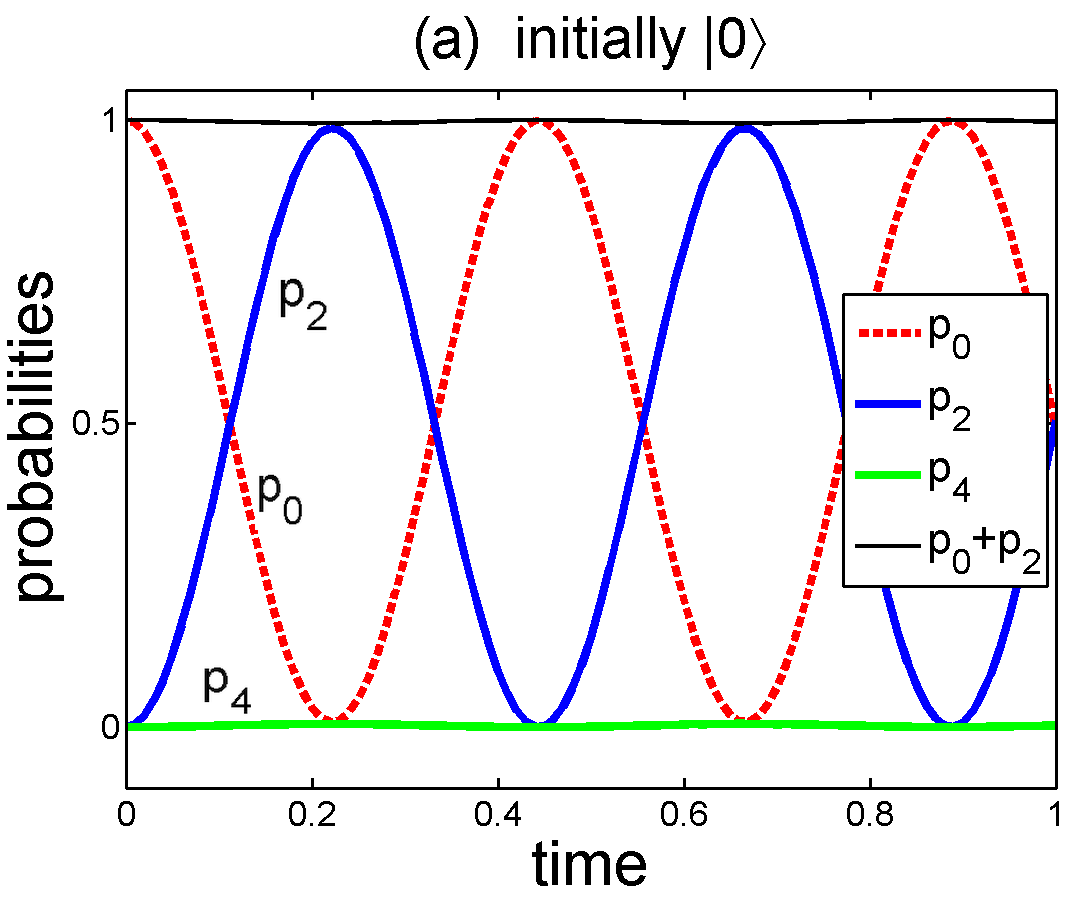
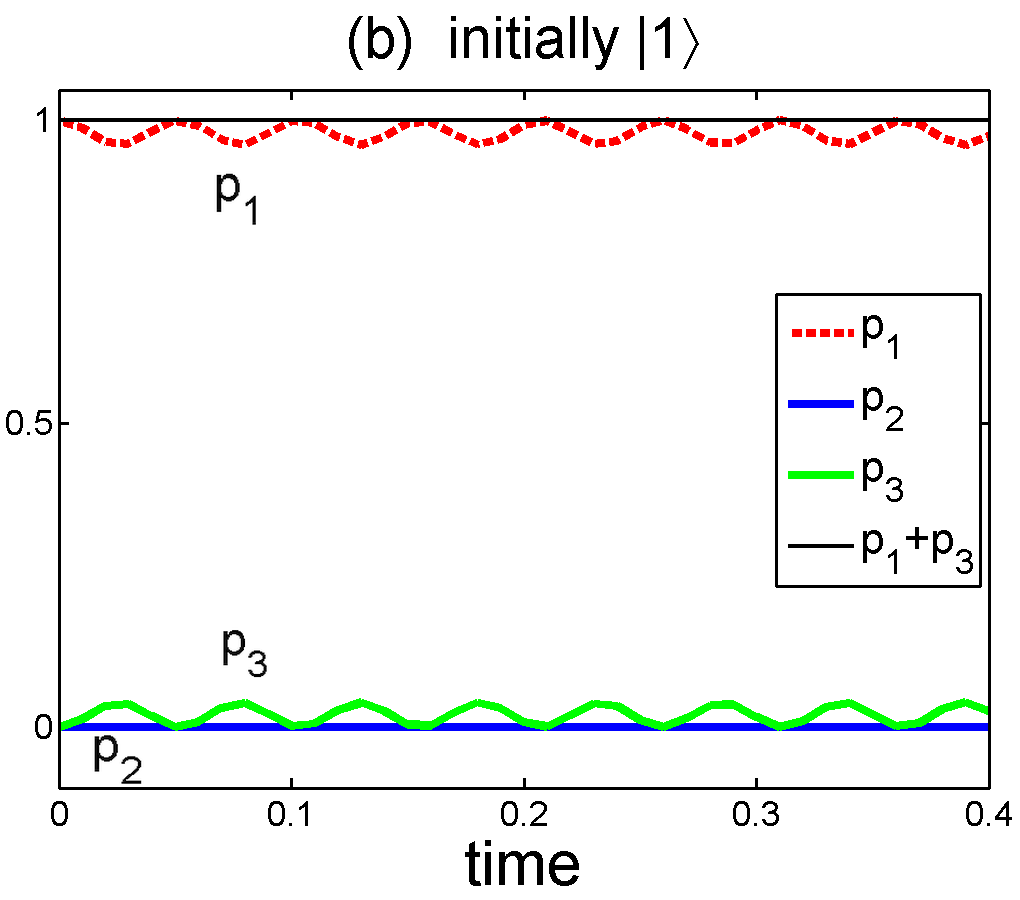
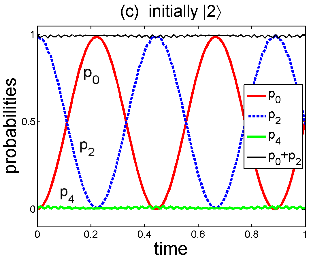
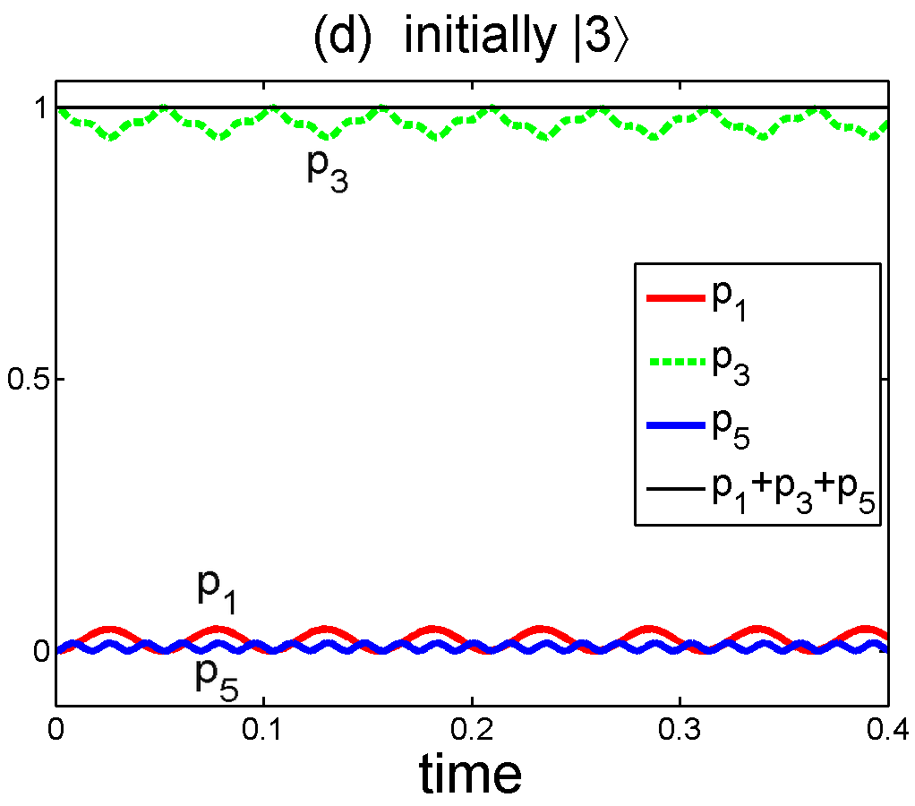
Figure 1: (Color online) Model 1: Dissipation-free evolution of the photon-number probabilities $p_{n}(t)=|\langle n{\,|\psi^{(m)}_{02}(t)\rangle}|^{2}$ and the photon-blockade fidelities $F(t)=\sum_{n}p_{n}(t)$ for the Hamiltonian $\hat{H}_{02}$, given by Eq. (14), for several initial Fock states ${\,|m\rangle}$ (as indicated in the panel titles). We set $\epsilon=\chi/6=5$. Panels (a) and (c) show Rabi-type oscillations between the levels ${\,|0\rangle}$ and ${\,|2\rangle}$, if at least one of them is initially populated. Rabi-type oscillations are not observed if the other levels are the only initially populated states, such as ${\,|1\rangle}$ and ${\,|3\rangle}$, as shown in panels (b) and (d), respectively. These results have a simple physical explanation in terms of the resonances shown in Fig. 2.

Figure 2: (Color online) Model 1: Explanation of the occurrence of photon blockade via the energy levels of the Hamiltonian $\hat{H}$ corresponding to $\hat{H}_{\rm s}(\Omega_{02}=\Omega,\Sigma_{02}=0)$, given by Eq. (12), in the limit of a very small driving strength, $\epsilon\ll\chi$. The Kerr-nonlinear term, proportional to $\chi$, changes the harmonic spectrum (shown in the left spectrum) into an anharmonic non-equidistant one (right side) with $E_{n+1}-E_{n}\neq\;$const, where $E_{n}=n\hbar\Omega+n(n-2)\hbar\chi$ (with $n=0,1,...)$ are the eigenvalues of the Hamiltonian $\hat{H}$. It is seen that the two-photon transitions between the levels $|0\rangle$ and $|2\rangle$ (shown by a solid double arrow in the right spectrum) can be induced by a driving field with frequency $\omega_{\rm d}=(E_{2}-E_{0})/\hbar=2\Omega$, which is the same as for the harmonic system. The other transitions between the levels, e.g., $|1\rangle$ and $|3\rangle$, as well as $|2\rangle$ and $|4\rangle$ (as shown by the dashed double arrows) are off-resonance with $\Omega$ or its multiples.

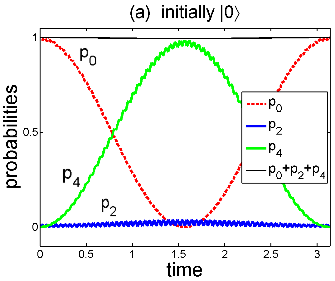
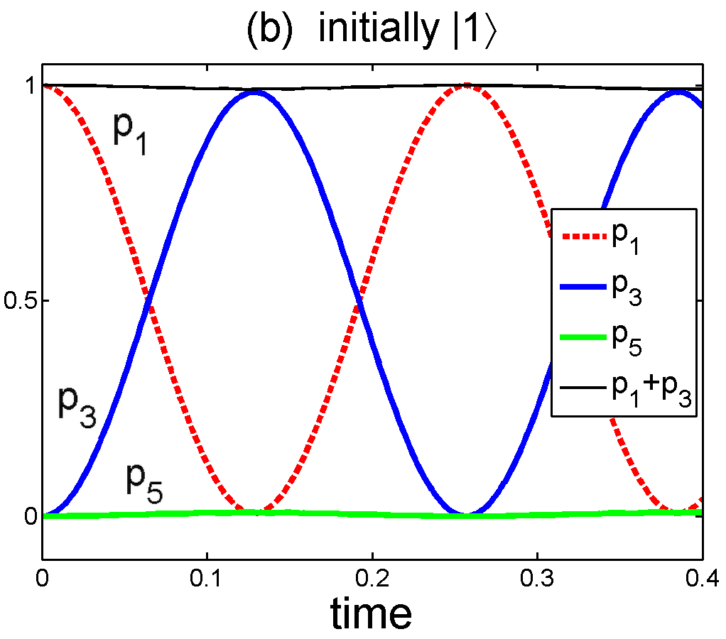
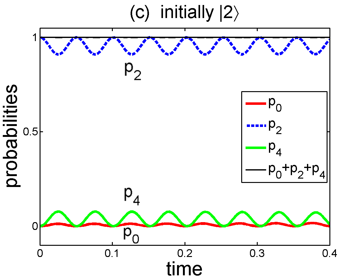
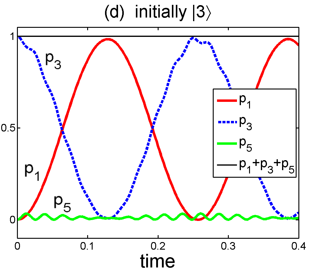
Figure 3: (Color online) Model 2: Same as in Fig. 1, but for the probabilities $p_{n}(t)=|\langle n{\,|\psi^{(m)}_{13}(t)\rangle}|^{2}$ obtained for the Hamiltonian $\hat{H}_{13}$, given by Eq. (17) with $k=1,l=3$. Panel (a) [(b) and (d)] show Rabi-type oscillations between the levels ${\,|0\rangle}$ and ${\,|4\rangle}$ (${\,|1\rangle}$ and ${\,|3\rangle}$), if at least one of these levels is initially populated. Rabi-type oscillations are not observed if the other levels are the only ones, which are initially populated, such as ${\,|2\rangle}$, shown in panel (c). The physical meaning of these results, analogously to those in Fig. 1, can be simply understood in terms of the resonances shown in Fig. 4.

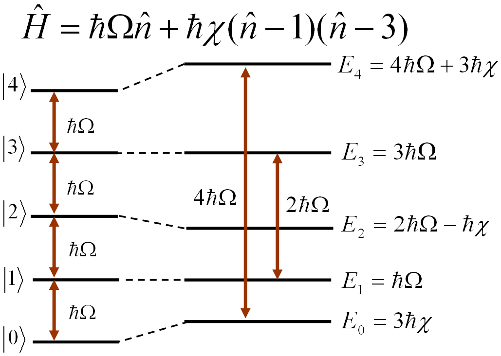
Figure 4: (Color online) Model 2: Same as in Fig. 2, but for the Hamiltonian $\hat{H}$ corresponding to $\hat{H}_{\rm s}(\Omega_{13}=\Omega,\Sigma_{13}=0)$, given by Eq. (15) with $k=1,l=3$ assuming $\epsilon\ll\chi$. Here the two-photon (four-photon) transitions between the levels $|1\rangle$ and $|3\rangle$ ($|0\rangle$ and $|4\rangle$), shown by solid double arrows in the right spectrum, can be induced by a driving field with frequency $\omega_{\rm d}=(E_{3}-E_{1})/\hbar=2\Omega$ [$\omega_{\rm d}=(E_{4}-E_{0})/\hbar=4\Omega$], which are the multiples of the same frequency $\Omega$ of the harmonic system.

III Nonstationary photon blockades and Rabi-type oscillations

Here we briefly describe the evolution of the systems described by Models 1 and 2 for some initial Fock states assuming no dissipation. These evolutions lead to time-dependent PB (or nonstationary PB), which can also be interpreted as an optical-state truncation.

Assuming that the driving field strength $\epsilon$ is much weaker than the Kerr nonlinearity $\chi$, one can find that the pure-state evolution of the system, described by the Hamiltonian $\hat{H}_{02}$ (Model 1), from the initial Fock states ${\,|0\rangle}$ and ${\,|2\rangle}$ can be approximately given as follows

$${\,|\psi^{(0)}_{02}(t)\rangle} \approx \cos(\sqrt{2}\epsilon t){\,|0\rangle}-i\sin(\sqrt{2}\epsilon t){\,|2\rangle},$$

$${\,|\psi^{(2)}_{02}(t)\rangle} \approx -i\sin(\sqrt{2}\epsilon t){\,|0\rangle}+\cos(\sqrt{2}\epsilon t){\,|2\rangle},$$ (22)

respectively. These solutions are in a very good agreement with the precise numerical solutions plotted in Figs. 1(a) and 1(c). In the derivation of Eq. (22), we have ignored the contribution of $(\epsilon/\chi)^{2}$. The solution ${\,|\psi^{(0)}_{02}(t)\rangle}$ can be referred to as a three-dimensional squeezed vacuum Miran96 or qutrit squeezed vacuum.

The solutions in Eq. (22) can be interpreted as Rabi-type oscillations between the states ${\,|0\rangle}$ and ${\,|2\rangle}$ in an artificial two-level system dynamically truncated (or generated) from the infinite-dimensional anharmonic system described by the Hamiltonian $\hat{H}_{02}$ for $\epsilon\ll\chi$. Thus, this phenomenon corresponds to a two-photon blockade, where the excitation of more than two photons is prohibited Miran13 . The evolutions shown in Figs. 1(b) and 1(d) are practically negligible. This photon blockade can be physically understood via the energy spectrum and resonances shown in Fig. 2. Note that our model, which leads to two-photon blockade induced by two-photon driving, differs from that in Ref. Miran13 , where a single-photon driving was assumed. We also mention that the state ${\,|2\rangle}$ in the solution ${\,|\psi^{(0)}_{13}(t)\rangle}$ is not populated, which is in contrast to the dissipative evolution analyzed in the next section (see Table I for comparison).

The dissipation-free system, given by the Hamiltonian $\hat{H}_{13}$ (Model 2), evolves from the initial Fock states ${\,|m\rangle}$ (for $m=0,1,3,4)$ as follows:

$${\,|\psi^{(0)}_{13}(t)\rangle} \approx \cos(\tfrac{1}{5}\epsilon t){\,|0\rangle}-i\sin(\tfrac{1}{5}\epsilon t){\,|4\rangle},$$

$${\,|\psi^{(1)}_{13}(t)\rangle} \approx \cos(\sqrt{6}\epsilon t){\,|1\rangle}-i\sin(\sqrt{6}\epsilon t){\,|3\rangle},$$

$${\,|\psi^{(3)}_{13}(t)\rangle} \approx -i\sin(\sqrt{6}\epsilon t){\,|1\rangle}+\cos(\sqrt{6}\epsilon t){\,|3\rangle},$$

$${\,|\psi^{(4)}_{13}(t)\rangle} \approx -i\sin(\tfrac{1}{5}\epsilon t){\,|0\rangle}+\cos(\tfrac{1}{5}\epsilon t){\,|4\rangle},$$ (23)

respectively. These are relatively good approximations of our precise numerical solutions plotted in Figs. 3(a), 3(b), and 3(d). In the derivations of these approximate solutions for ${\,|\psi^{(n)}_{13}(t)\rangle}$, the same as for ${\,|\psi^{(n)}_{02}(t)\rangle}$, the contribution of $(\epsilon/\chi)^{2}$ was omitted.

We interpret the solutions in Eqs. (23) analogously to those in Eqs. (22), i.e., as generalized two-photon (four-photon) blockades and Rabi-type oscillations between the states ${\,|1\rangle}$ and ${\,|3\rangle}$ (${\,|0\rangle}$ and ${\,|4\rangle}$) in an artificial two-level system dynamically truncated from the infinite-dimensional system of the Hamiltonian $\hat{H}_{13}$ if $\epsilon\ll\chi$. The contributions of other Fock states are practically negligible, as seen in Figs. 3. These phenomena can be easily understood by analyzing the energy spectra and resonances shown in Fig. 4.

For a comparison, we also recall the well-known approximate solutions for the pure-state evolutions, under the interaction described by the Hamiltonian $\hat{H}_{\rm usual}$ Leonski94 :

$${\,|\psi^{(0)}_{\rm usual}(t)\rangle} \approx \cos(\epsilon t){\,|0\rangle}-i\sin(\epsilon t){\,|1\rangle},$$

$${\,|\psi^{(1)}_{\rm usual}(t)\rangle} \approx -i\sin(\epsilon t){\,|0\rangle}+\cos(\epsilon t){\,|1\rangle},$$ (24)

assuming the initial vacuum and single-photon states, respectively. These solutions can be interpreted as single-photon blockade in the dissipation-free regime and two-dimensional (or qubit) coherent states Miran94 .

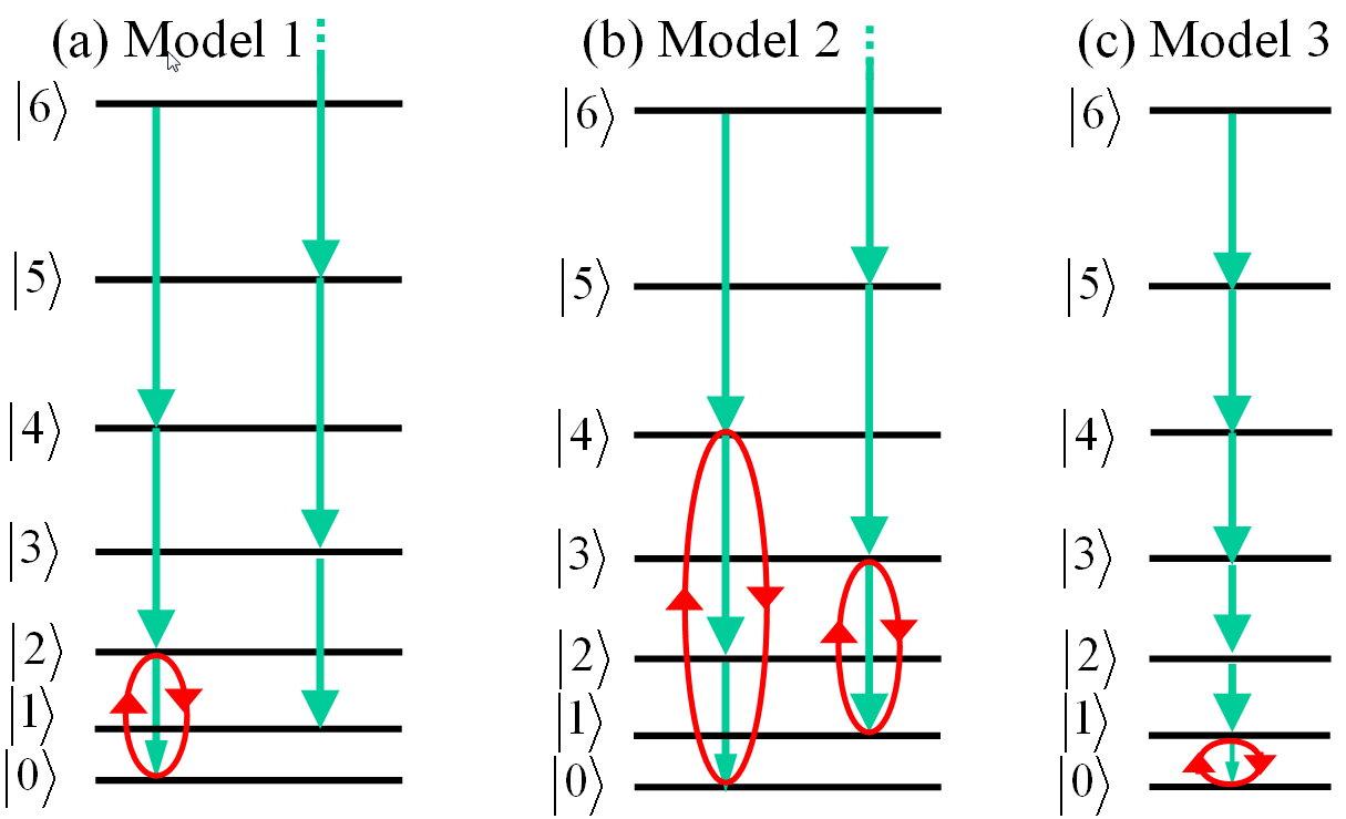
Figure 5: (Color online) An intuitive explanation of the engineered photon blockades in Models 1 and 2 with two-photon dissipation, and the standard photon blockade in Model 3 with single-photon dissipation. The diagrams schematically show the energy levels of three Kerr-type nonlinear systems driven by a classical field with frequency $\omega_{\rm d}$ in resonance with the desired transitions, as shown in Fig. 2 for Model 1 and Fig. 4 for Model 2. The red ellipses with arrows describe these [(a),(b)] two-photon and (c) single-photon drivings, together with the Rabi-type oscillations between the corresponding levels. The systems are described by the Hamiltonians: (a) $\hat{H}_{02}$, given by Eq. (14), (b) $\hat{H}_{13}$, given by Eq. (17) for $k=1,l=3$, and $\hat{H}_{\rm usual}$, given by Eq. (20). The system dissipation is governed by the master equations describing either [(a), (b)] two-photon or (c) single-photon absorption for $\gamma\ll\epsilon\ll\chi$. The numerous green single arrows pointing down describe these dissipations (absorptions). These figures intuitively explain the occurrence of several kinds of the engineered photon blockades, as well as two independent evolutions of the initial Fock states with even and odd numbers of photons for Models 1 and 2. This implies that the engineered PB effects in panels (a,b) can depend on the initial state of a cavity, although in a limited way, as they depend solely on the ratio of the probabilities of measuring the photon numbers of different parity. In contrast to this, the steady state generated in standard PB, as shown in (c), is independent of the cavity initial state.

IV Steady-state photon blockades via two-photon dissipation

Here we explain in detail the occurrence of various kinds of steady-state engineered PB effects, when the systems described by the Hamiltonians $\hat{H}_{02}$ and $\hat{H}_{13}$ are affected by two-photon loss mechanisms, as schematically shown in Fig. 5.

IV.1 Master equation describing two-photon absorption

We assume that the system (s), described by the Hamiltonian $\hat{H}_{kl}$, is coupled to an engineered reservoir (r) via two-photon processes (see, e.g., Refs. Simaan78 ; Gilles93 ; Gilles94 ; Guerra97 ; Dodonov97 ; Everitt13 ; Ispasoiu00 ; Klimov03 ; Buks06 ; Yurke06 ; Karasik08 ; Boissonneault12 ; Voje13 ; Albert14 ) as described by $\hat{H}=\hat{H}_{\rm s}+\hat{H}_{\rm r}+\hat{H}_{\rm sr},$ where

$$\hat{H}_{\rm sr}=\hbar g_{\rm sr}[\hat{a}^{2}\hat{\Gamma}^{\dagger}+(\hat{a}^{\dagger})^{2}\hat{\Gamma}],$$ (25)

and $\hat{H}_{\rm r}$ can be given, depending on the physical realization, by, e.g., $\hbar\sum_{n}\omega_{n}\hat{\sigma}_{z}^{(n)}$ or $\hbar\sum_{n}\omega_{n}\hat{a}_{n}^{\dagger}\hat{a}_{n}$, while the collective reservoir annihilation operator $\hat{\Gamma}$ is given by $\sum_{n}\hat{\sigma}_{-}^{(n)}$ or $\sum_{n}\hat{a}_{n}$, respectively. Moreover, $g_{\rm sr}$ is the system-reservoir coupling strength; $\omega_{n}$ is the frequency of the $n$th mode of the reservoir, $\hat{\sigma}_{z}^{(n)}$ and $\hat{\sigma}_{-}^{(n)}$ are the spin operators for the $n$th qubit, defined analogously to those below Eq. (5), and $\hat{a}_{n}$($\hat{a}_{n}^{\dagger}$) is the annihilation (creation) operator of the $n$th mode of the reservoir. Thus, the evolution, under the Markov approximation, of the reduced density matrix for the system can be given by the following two-photon-absorption master equation in the Lindblad form assuming zero temperature of the reservoir Simaan78 ; Gilles93 ; Guerra97 ; Karasik08 ,

$$\frac{d\hat{\rho}}{dt}={\cal L}\hat{\rho}\equiv\ -\frac{i}{\hbar}[\hat{H}_{\rm s},\hat{\rho}]+\gamma{\cal D}[\hat{a}^{2}]\hat{\rho},$$ (26)

where the superoperator ${\cal D}$ is defined by ${\cal D}[\hat{L}]\hat{\rho}=\hat{L}\hat{\rho}\hat{L}^{{\dagger}}-\frac{1}{2}(\hat{L}^{\dagger}\hat{L}\hat{\rho}+\hat{\rho}\hat{L}^{{\dagger}}\hat{L})$, and ${\cal L}$ is sometimes referred to as the Liouvillian (or Lindbladian) superoperator. Moreover, $\gamma=\gamma_{2}$ is the two-photon damping constant (two-photon decay rate).

It is worth noting that a single-mode squeezed state can be generated by this two-photon absorption process via pure dissipation Gilles93 . This can be readily concluded by noting that the Hamiltonian in Eq. (25) corresponds to a prototype squeezing Hamiltonian in the parametric approximation, when the collective reservoir operator $\hat{\Gamma}$ is treated classically. Thus, Eq. (26) can be considered a master equation obtained for a squeezing-generating reservoir. Note that this equation is completely different from the standard master equation for an amplifier whose reservoir consists of squeezed white noise (squeezed-vacuum reservoir) ScullyBook .

A more general form of the master equation can read Everitt13

$$\frac{d\hat{\rho}}{dt}={\cal L^{\prime}}\hat{\rho}=-\frac{i}{\hbar}[\hat{H}_{\rm s},\hat{\rho}]+\gamma_{\perp}{\cal D}[\hat{a}^{\dagger}\hat{a}]\hat{\rho}+\gamma_{1}{\cal D}[\hat{a}]\hat{\rho}+\gamma_{2}[\hat{a}^{2}]\hat{\rho},$$ (27)

to include also single-photon absorption with its decay rate $\gamma_{1}$, and pure dephasing with its rate $\gamma_{\perp}$, in addition to two-photon absorption. Note that it is still assumed in this equation that the reservoir is at zero temperature, so there is no transfer of reservoir fluctuations into the system.

Our former studies Liu10 ; Miran13 showed that the standard realizations of photon blockade can be very sensitive to these thermal fluctuations. Nevertheless, for simplicity, we apply here the zero-temperature master equations, given by Eq. (26) or, equivalently, by Eq. (27) assuming that

$$0\approx\gamma_{\perp}\approx\gamma_{1}\ll\gamma_{2}\ll\epsilon\ll\chi.$$ (28)

In order to visualize the steady-state solutions of the two-photon-loss master equation, given by Eqs. (26), we plot their Wigner functions and photon-number probabilities $p_{n}=\langle n|\hat{\rho}_{{\rm ss}}|n\rangle$ in Figs. 6–13. Moreover, Fig. 14 shows analogous solutions of the single-photon-loss master equation, given in Eq. (27) assuming that the single-photon decay rate $\gamma_{1}$ is dominantly larger than the two-photon decay rate $\gamma_{2}$ and the dephasing rate $\gamma_{\perp}$.

IV.2 Steady-state solutions of the master equation

Now we present our precise numerical and approximate analytical steady-state solutions of the two-photon absorption master equation, given by Eq. (26), to show explicitly how photon blockade in the discussed engineered reservoir depends on initial states.

Steady-state solutions $\hat{\rho}_{{\rm ss}}$ can be obtained by solving the master equation, given in Eqs. (26) and (27), with the condition $\frac{\rm d}{dt}\hat{\rho}_{{\rm ss}}\equiv\frac{\rm d}{dt}\hat{\rho}=0$, by using, e.g., the inverse power method (as implemented, e.g., in Ref. Tan99 ) or by a direct integration, for long enough evolution times: $\hat{\rho}_{{\rm ss}}=\hat{\rho}(t\rightarrow\infty)$. All our numerical results, shown in Figs. 6–14, are based on these two equivalent methods. We also applied an analytical approach of finding approximate solutions of the master equation, given in Eq. (26), as described below.

We assume that the ratio of the driving field strength $\epsilon$ and the Kerr nonlinear coupling $\chi$, and the ratio of $\chi$ and the damping constant $\gamma$ are small, i.e., $\delta=\epsilon/\chi\ll 1$ and $\delta^{\prime}=\gamma/\epsilon\ll 1$. Thus, we can analyze the cavity-field Hilbert space of a small dimension. For example, let us truncate the Hilbert space at the five-photon Fock state, which corresponds to analyzing a six-dimensional Hilbert space. We have obtained numerically a very good agreement between our numerical solutions in the six- and 100-dimensional Hilbert spaces for the parameters chosen in all figures.

In order to find compact-form analytical solutions, we expanded our lengthy and complicated solutions (which are not presented here) in power series of $\delta$ and $\delta^{\prime}$, and keeping linear and quadratic terms only.

First, let us assume the initial state of our system is an even-number state, i.e.,

$$\hat{\rho}_{0,\rm even}=\sum_{m=1}^{\infty}p_{m}{\,|\psi_{m}\rangle}{\langle\psi_{m}|\,},\quad{\,|\psi_{m}\rangle}=\sum_{n=0}^{\infty}c_{n}^{(m)}{\,|2n\rangle},$$ (29)

with arbitrary probabilities $p_{m}$ and complex amplitudes $c_{n}^{(m)}$, satisfying the normalization conditions $\sum_{m}p_{m}=\sum_{n}|c_{n}^{(m)}|^{2}=1$, for $m=1,2,...\,$. Then we find the steady-state solutions of the master equation, given by Eq. (26), for the system described by the Hamiltonians $\hat{H}_{02}$ and $\hat{H}_{13}$, to be given, in the standard Fock basis, by

$$\hat{\rho}^{{\rm even}}_{{\rm ss}}\approx\left[\begin{array}[]{cccccc}p&0&a+ib&0&c+id&0\\ 0&0&0&0&0&0\\ a-ib&0&q&0&e+if&0\\ 0&0&0&0&0&0\\ c-id&0&e-if&0&r&0\\ 0&0&0&0&0&0\end{array}\right]$$ (30)

in terms of the coefficients given explicitly in Appendix A. By further assuming that $\delta^{2}\approx\delta^{\prime 2}\approx\delta\delta^{\prime}\approx 0$ then $r\approx c\approx d\approx f=0$ for Model 1 [see Eqs. (55) and (56)]. Thus, it is seen that the steady state, which can be generated in this model, assuming that the cavity field is initially in an even-number state, is a partially incoherent superposition of effectively only two number states, ${\,|0\rangle}$ and ${\,|2\rangle}$, while for Model 2, the steady state is spanned by the number states${\,|0\rangle}$, ${\,|2\rangle}$, and ${\,|4\rangle}$. See Table I for comparison.

Now we assume that the initial state of our system is an odd-number state, i.e.,

$$\hat{\rho}_{0,\rm odd}=\sum_{m=1}^{\infty}p_{m}{\,|\psi_{m}\rangle}{\langle\psi_{m}|\,},\quad{\,|\psi_{m}\rangle}=\sum_{n=0}^{\infty}c_{n}^{(m)}{\,|2n+1\rangle},\$$ (31)

for any $p_{m}$ and $c_{n}^{(m)}$, as in Eq. (29). Then the steady-state solution for $\hat{H}_{02}$ and $\hat{H}_{13}$ can be approximately given by

$$\hat{\rho}^{{\rm odd}}_{{\rm ss}}\approx p|1\rangle\langle 1|+(1-p)|3\rangle\langle 3|+[(a+ib)|1\rangle\langle 3|+{\rm h.c.}].$$ (32)

where the coefficients $a$, $b$, and $p$ are given explicitly in Appendix A. It is seen that the steady state is spanned by the number states ${\,|1\rangle}$ and ${\,|3\rangle}$ only. Actually, by also ignoring the terms proportional to $\delta^{2}$, $\delta^{\prime 2}$, and $\delta\delta^{\prime}$, the steady state for Model 1 is just the single-photon state, which is not the case for Model 2 (see also Table I for comparison).

As an illustration of these results, the Wigner functions and photon-number probabilities for the numerically calculated steady-state solutions $\hat{\rho}^{{\rm even}}_{{\rm ss}}$ and $\hat{\rho}^{{\rm odd}}_{{\rm ss}}$ are shown in Figs. 6 and 7. On the scale of these plots, there is practically no difference between our approximate analytical and precise numerical solutions. Figure 8 shows how the steady-state number probabilities $p_{n}$ depend on the driving field strength $\epsilon$ in units of the damping constant $\gamma$ for an initial even-number state. Analogous solutions for an initial odd-number state practically do not depend on $\epsilon/\gamma\in[0,10]$. Figure 9 shows how the probabilities $p_{n}$ depend on the tuning frequencies $\Omega_{02}$ (assuming $\Sigma_{02}=0$) and $\Omega_{13}$ (with $\Sigma_{13}=0$).

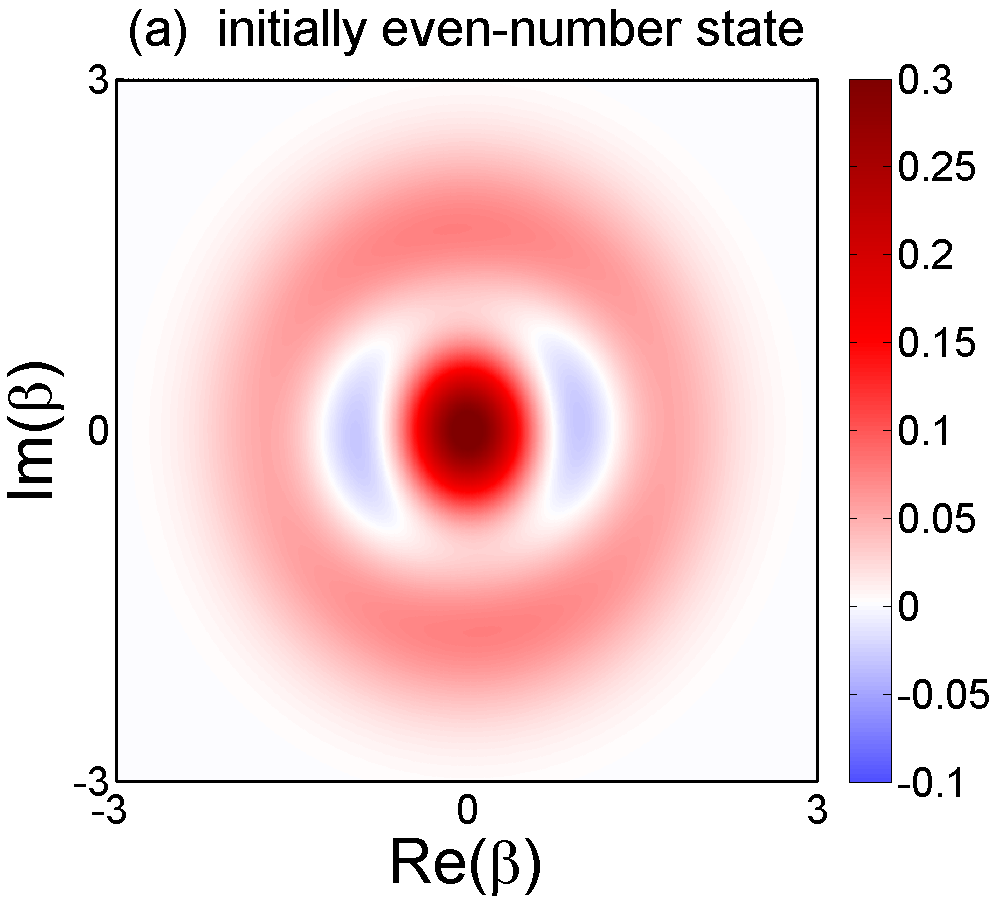
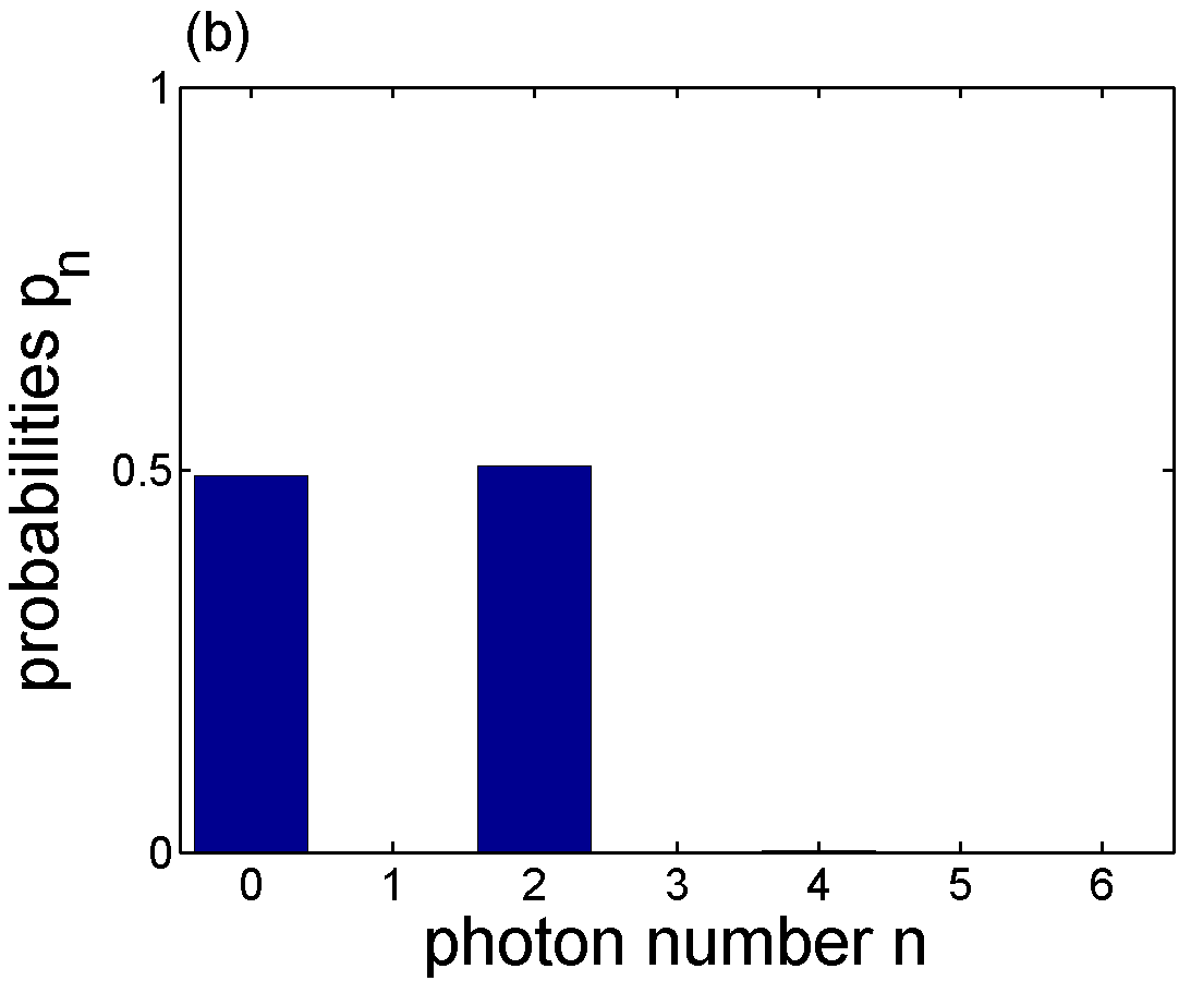
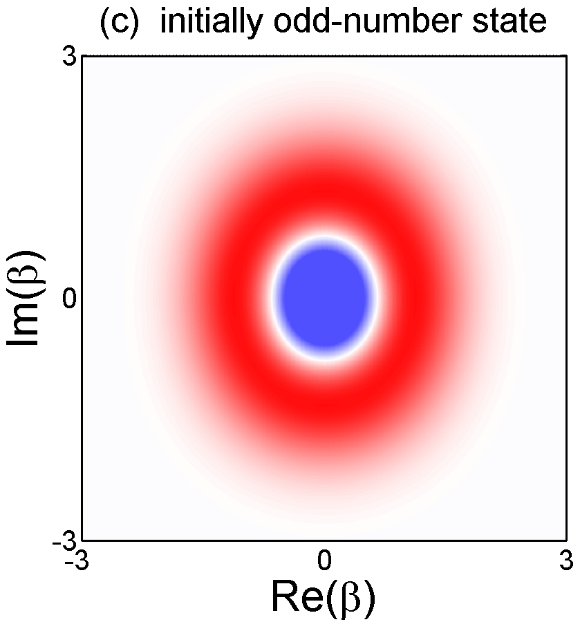
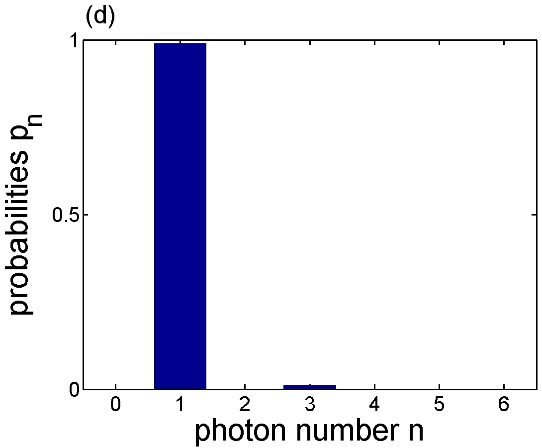
Figure 6: (Color online) Model 1 with two-photon dissipation: (a,c) The Wigner functions $W(\beta)$ and (b,d) the photon-number probabilities $p_{n}$ for the steady-state solutions $\hat{\rho}^{02}_{{\rm ss}}$ of the master equation (26) with the Hamiltonian $\hat{H}_{02}$, given by Eq. (14), assuming the cavity field to be initially in an arbitrary (a,b) even- or (c,d) odd-number state. We set the ratios of the driving field strength $\epsilon$ and the Kerr nonlinear coupling $\chi$, and of the damping constant $\gamma$ and $\epsilon$ to be small and equal to $\delta=\epsilon/\chi=1/6$ and $\delta^{\prime}=\gamma/\epsilon=1/25$. The color codes in panel (c) (and all other figures of the Wigner functions) are the same as in panel (a). Note that the negative regions of the Wigner functions are marked in blue.

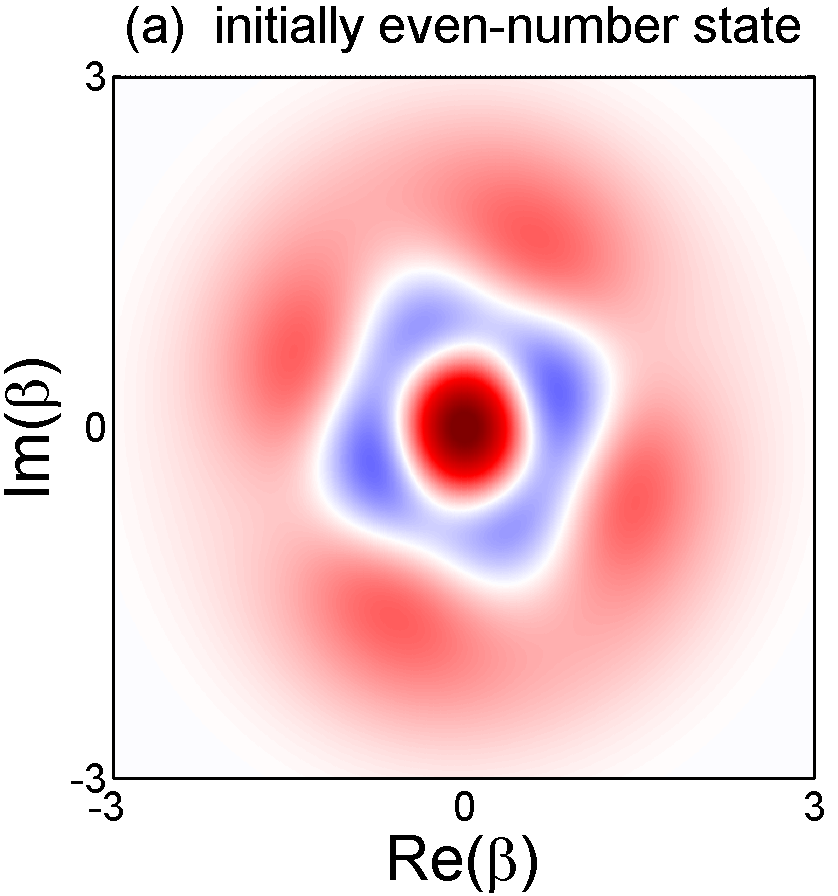
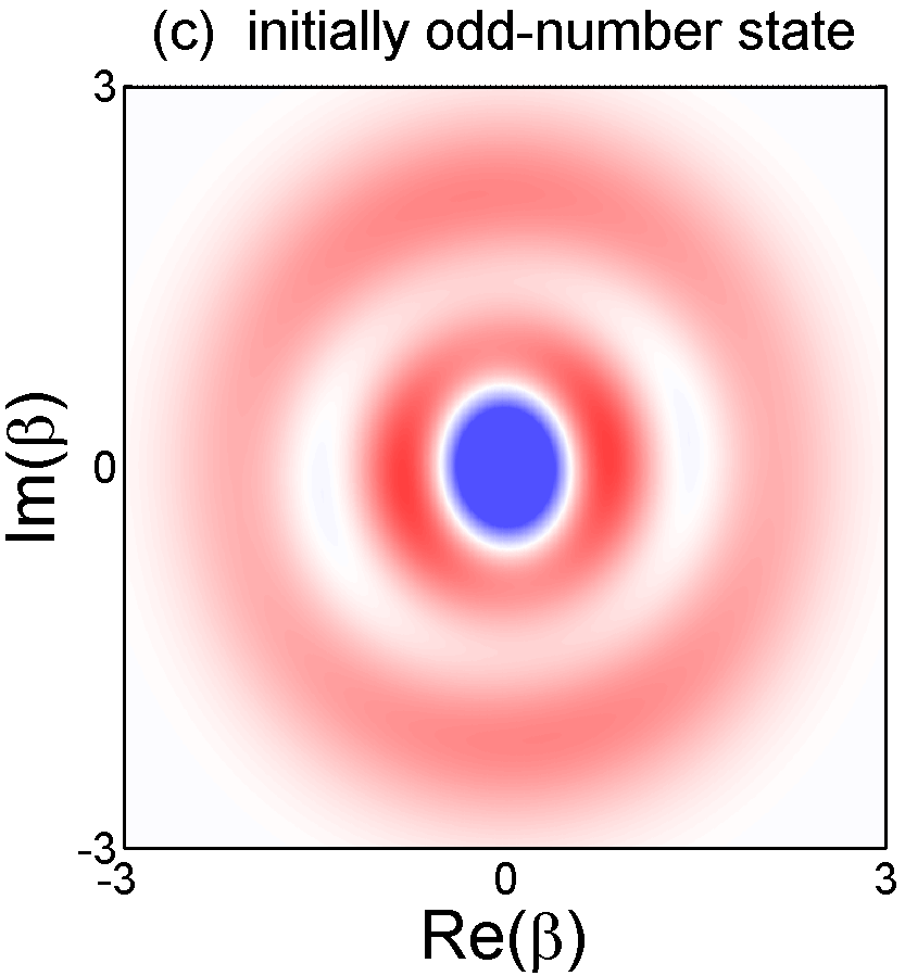
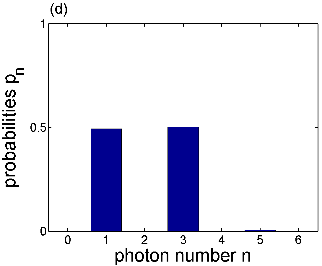
Figure 7: (Color online) Model 2 with two-photon dissipation: Same as in figure 6, but for the steady-state solutions $\hat{\rho}^{13}_{{\rm ss}}$ of the master equation (26) with the Hamiltonian $\hat{H}_{13}$, given by Eq. (17) for $k=1,l=3$.

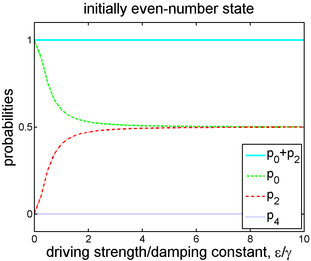
Figure 8: (Color online) Model 1 with two-photon dissipation: The photon-number probabilities $p_{n}={\langle n|\,}\hat{\rho}^{02}_{{\rm ss}}{\,|n\rangle}$ and the fidelity $F=p_{0}+p_{2}$ of the photon blockade versus the driving field strength $\epsilon$, in units of the damping constant $\gamma$, assuming the initial state to have an even number of photons and $\gamma/\chi=1/150$. The analogous figure for an initial odd-number state is omitted since $p_{1}\approx 1$ [see Fig. 6(d)], at least, for $\epsilon/\gamma\in[0,10]$. For brevity, analogous plots for Model 2 are not presented here either.

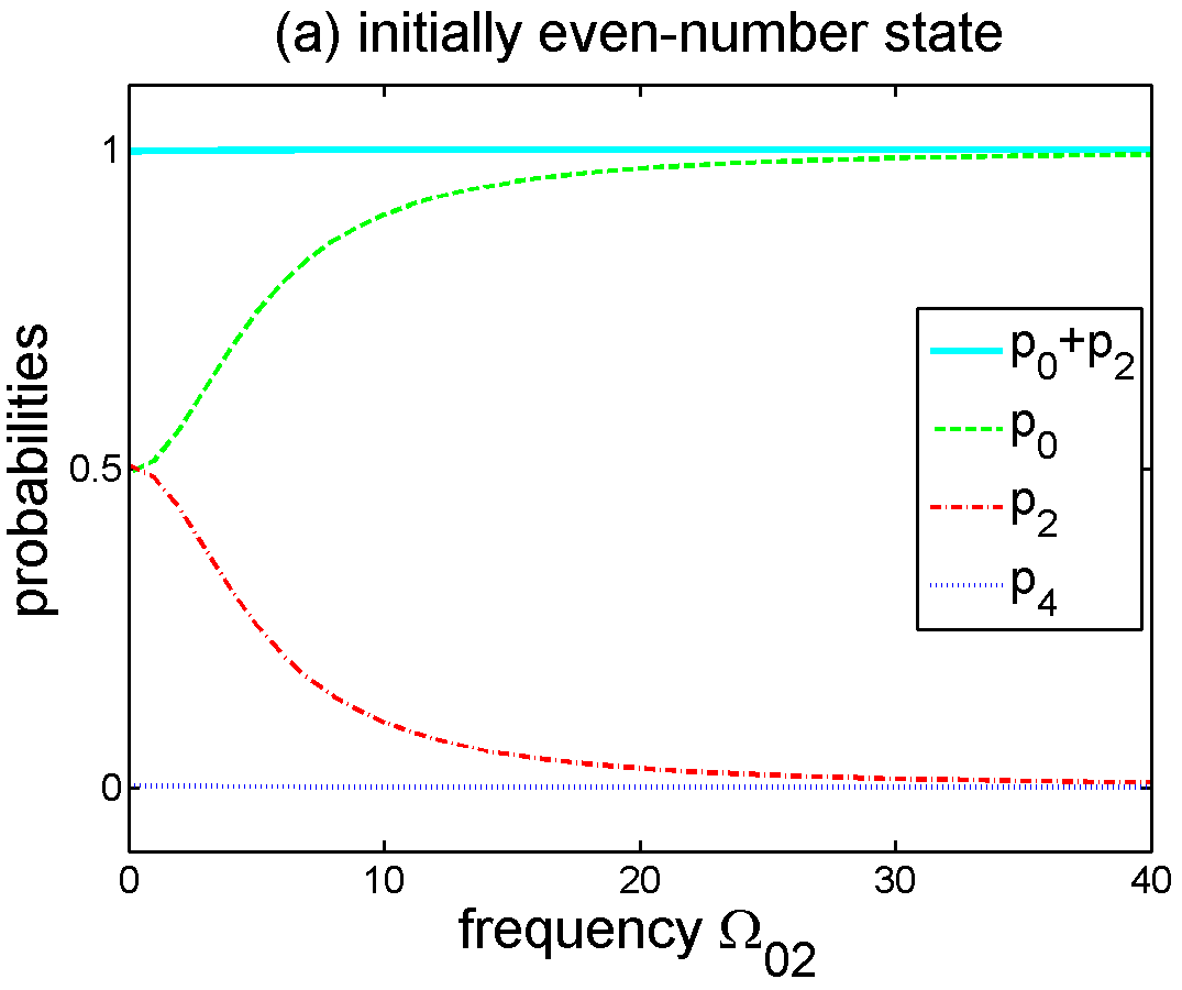
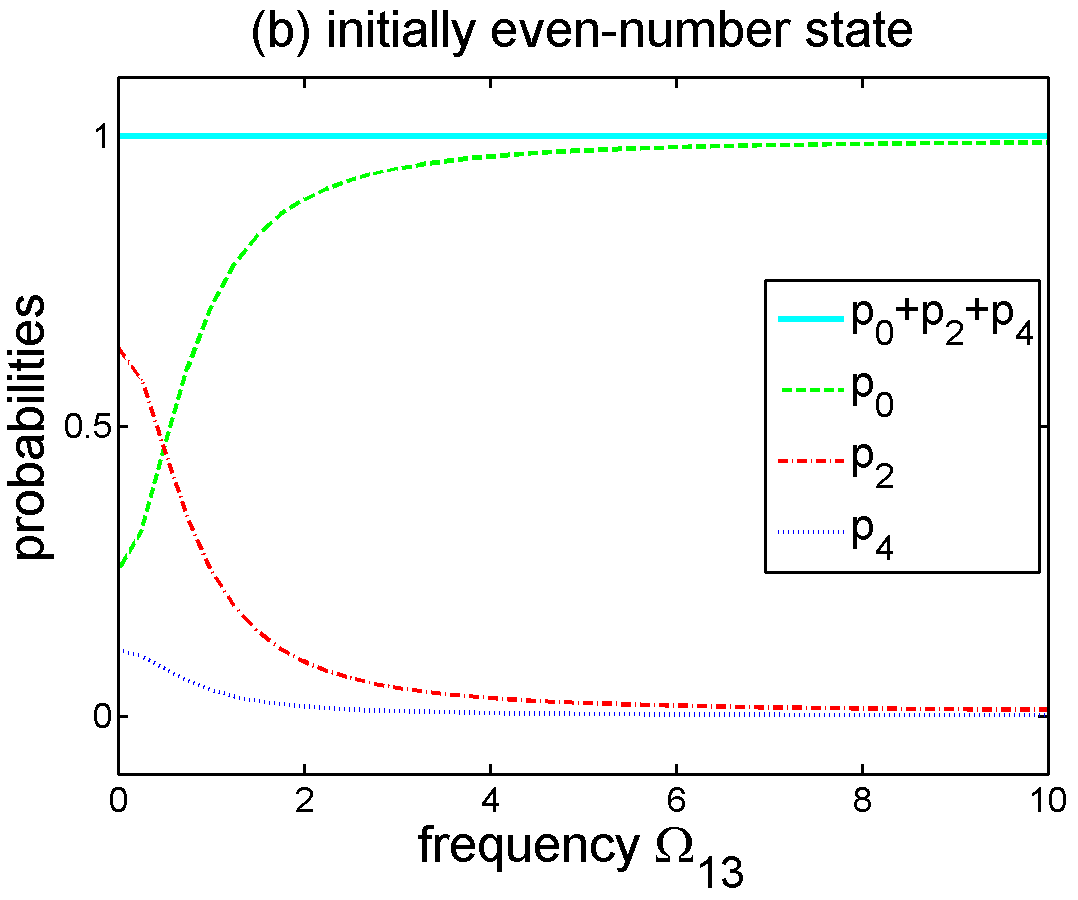
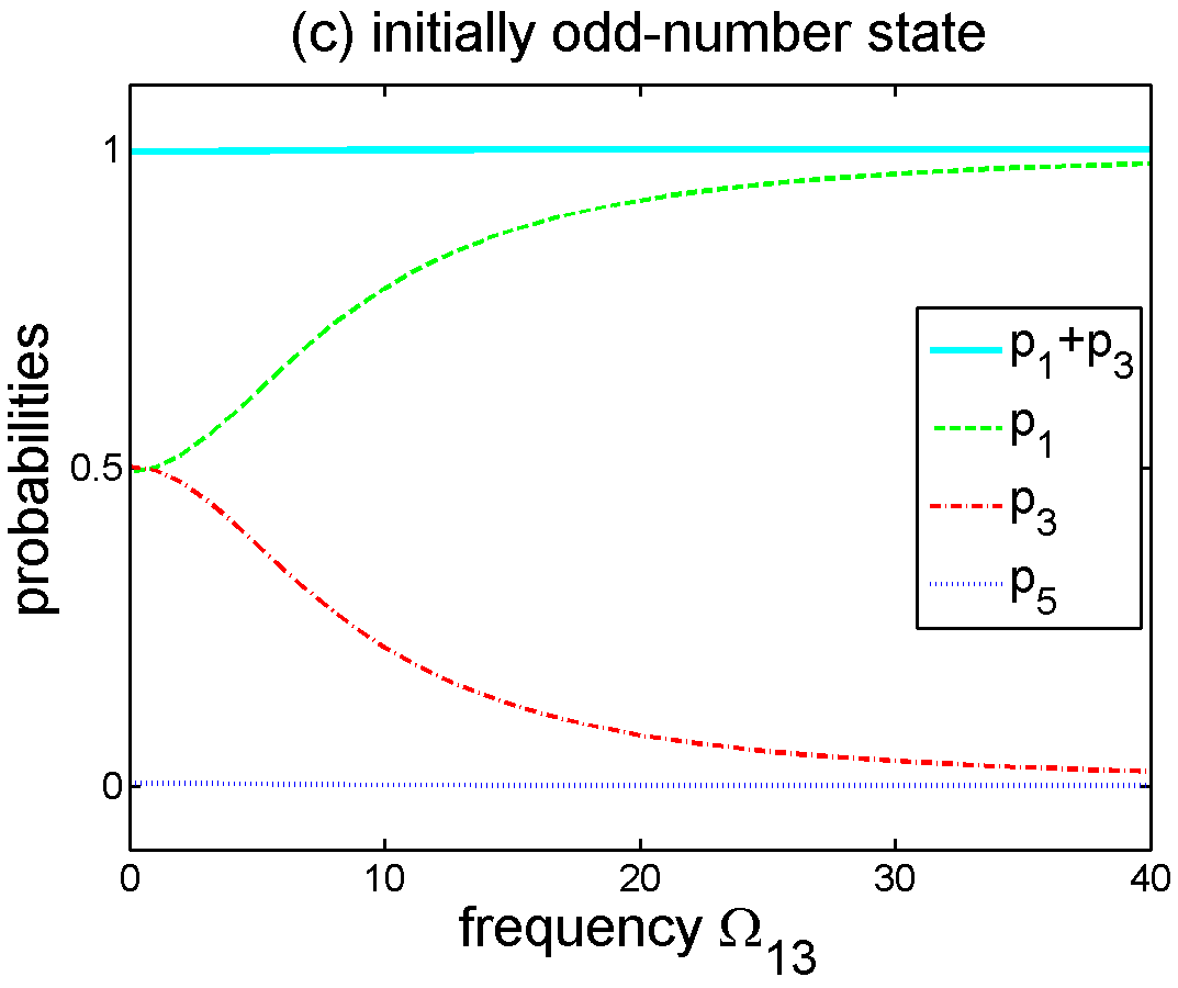
Figure 9: (Color online) Model 1 in panel (a) and Model 2 in (b,c) with two-photon dissipation: The photon-number probabilities $p_{n}$ and the fidelity $F=\sum_{n}p_{n}$ of the photon blockade versus the tuning frequency $\Omega_{kl}$ for the steady-state solutions $\hat{\rho}_{{\rm ss}}$ of the master equation (26), for the Hamiltonian $\hat{H}_{\rm s}(\Omega_{kl},\Sigma_{kl})$ with fixed $\Sigma_{kl}=0$, assuming the initial state to have (a,b) an even or (c) odd number of photons. Here we set $\delta=\epsilon/\chi=1/6$ and $\delta^{\prime}=\gamma/\epsilon=1/25$. The corresponding curves $p_{n}$ versus $\Omega_{02}$ for $\hat{H}_{\rm s}(\Omega_{02},\Sigma_{02}=0)$ and the initial state with odd number of photons are not presented here because $p_{1}\approx 1$ and $p_{3}\approx 0$ in the whole studied interval, and this is fully apparent from Fig. 6(d) as well. It is seen that even if $\Omega_{kl}\neq 0$, PB can still occur. Nevertheless, for an initial even (odd) number state, the output steady state approaches the vacuum (single-photon) state even for a relatively small $\Omega_{kl}$. Note that plots in panels (a) and (c) look very similar but they correspond to different probabilities.

We find that the steady-state solution of the master equation, given by Eq. (26) assuming $\gamma\ll\epsilon\ll\chi$, reads

$$\hat{\rho}_{{\rm ss}}(\hat{\rho}_{0})=p_{{\rm even}}(\hat{\rho}_{0})\hat{\rho}^{{\rm even}}_{{\rm ss}}+p_{{\rm odd}}(\hat{\rho}_{0})\hat{\rho}^{{\rm odd}}_{{\rm ss}},$$ (33)

for an arbitrary initial state $\rho_{0}$. This solution is a weighted sum of the steady-state solutions, given by Eqs. (30) and (32), with the weights

$$p_{{\rm even}}(\hat{\rho}_{0}) = \sum_{n=0}^{\infty}\langle 2n|\hat{\rho}_{0}|2n\rangle,$$ (34)

$$p_{{\rm odd}}(\hat{\rho}_{0}) = \sum_{n=0}^{\infty}\langle 2n+1|\hat{\rho}_{0}|2n+1\rangle.$$ (35)

So, it holds $p_{{\rm even}}(\hat{\rho}_{0})+p_{{\rm odd}}(\hat{\rho}_{0})=1$. It is seen that

$$\hat{\rho}^{{\rm even}}_{{\rm ss}} \equiv \hat{\rho}_{{\rm ss}}(\sum_{n}c_{n}|2n\rangle)=\hat{\rho}_{{\rm ss}}(|0\rangle),$$ (36)

$$\hat{\rho}^{{\rm odd}}_{{\rm ss}} \equiv \hat{\rho}_{{\rm ss}}(\sum_{n}c_{n}|2n+1\rangle)=\hat{\rho}_{{\rm ss}}(|1\rangle).$$ (37)

for any complex amplitudes $c_{n}$.

Our result that

$$\hat{\rho}_{{\rm ss}}(|0\rangle) \neq \hat{\rho}_{{\rm ss}}(|1\rangle)$$ (38)

sounds counterintuitive for the following reason: To find the solution of the master equation, given by Eq. (26), one can write separately the equations of motion for all the elements $\rho_{ij}(t)$ of the density matrix $\hat{\rho}(t)$. The steady-state solutions $\bar{\rho}^{\rm ss}_{ij}=\lim_{t\rightarrow\infty}\rho_{ij}(t)$ can be obtained by setting $\partial\bar{\rho}^{\rm ss}_{ij}/\partial t=0$. Then, it would appear that the elements $\bar{\rho}^{\rm ss}_{ij}$ in the steady state do not depend on the initial conditions. We will show below that they can depend on the initial states of mixed parity. Namely, let us create two matrices $\hat{\rho}^{\prime}$ and $\hat{\rho}^{\prime\prime}$ with the only nonzero elements $\rho^{\prime}_{2i,2j}=\bar{\rho}^{\rm ss}_{2i,2j}$ and $\rho^{\prime\prime}_{2i+1,2j+1}=\bar{\rho}^{\rm ss}_{2i+1,2j+1}$ for $i,j=0,1,...$. Then, the even steady-state density matrix, given by Eq. (36), simply reads as $\hat{\rho}^{\rm ss}_{\rm even}=\hat{\rho}^{\prime}/{\rm tr\,}(\hat{\rho}^{\prime})$. Analogously, the odd steady-state density matrix, given by Eq. (37), is equal to $\hat{\rho}^{\rm ss}_{\rm odd}=\hat{\rho}^{\prime\prime}/{\rm tr\,}(\hat{\rho}^{\prime\prime})$. The general solution, given in Eq. (33), is then state-dependent, although in this limited manner.

These formulas can be confirmed numerically by comparing them with the solutions for the master equation obtained for sufficiently long evolution times. Moreover, the steady-state density matrix elements $\bar{\rho}^{\rm ss}_{ij}$ can be directly calculated numerically by finding a vector in the null space of the Liouvillian superoperator ${\cal L}$ Tan99 .

We note that the ratio

$$r=\frac{p_{{\rm odd}}(\hat{\rho}_{0})}{p_{{\rm even}}(\hat{\rho}_{0})}=\frac{p_{{\rm odd}}(\hat{\rho}_{\rm ss})}{p_{{\rm even}}(\hat{\rho}_{\rm ss})}$$ (39)

is preserved during the system evolution. This is because the two-photon driving and two-photon dissipation, together with the photon-number-preserving Kerr interaction, do not mix even and odd number states. To show how this engineered photon blockade depends on the initial states $\hat{\rho}_{0}$, the ratio $r$ is plotted in Figs. 10–13 for a few states $\hat{\rho}_{0}$ discussed in the next section.

Finally, we note that these steady-state solutions, as well as our precise numerical solutions shown in all plots, depend solely on the ratios $\delta=\epsilon/\chi$ and $\delta^{\prime}=\gamma/\epsilon$, and do not depend on the absolute values of $\epsilon$, $\chi$, and $\gamma$.

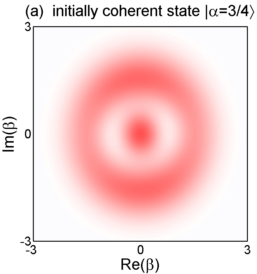
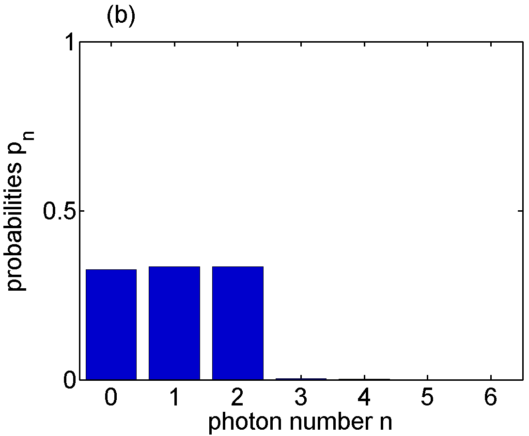
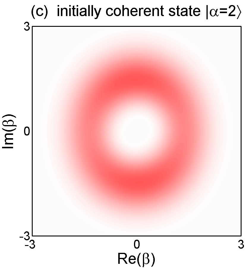
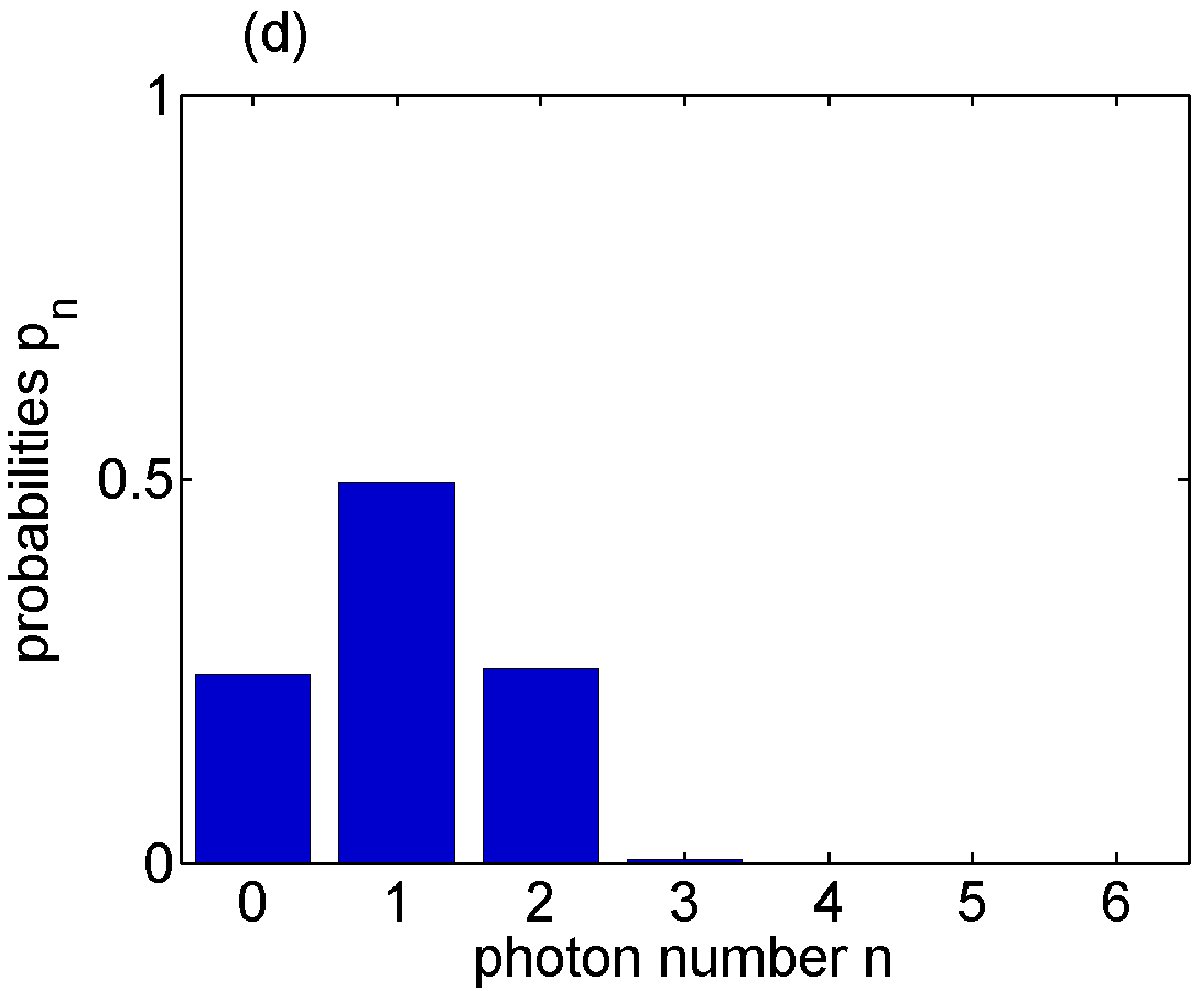
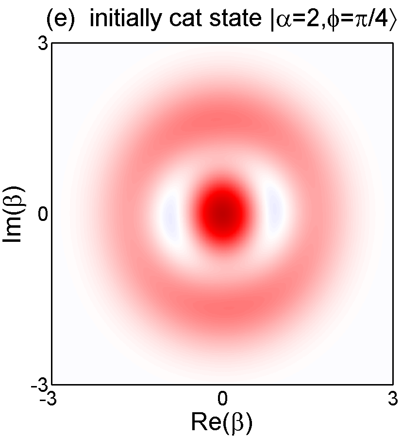
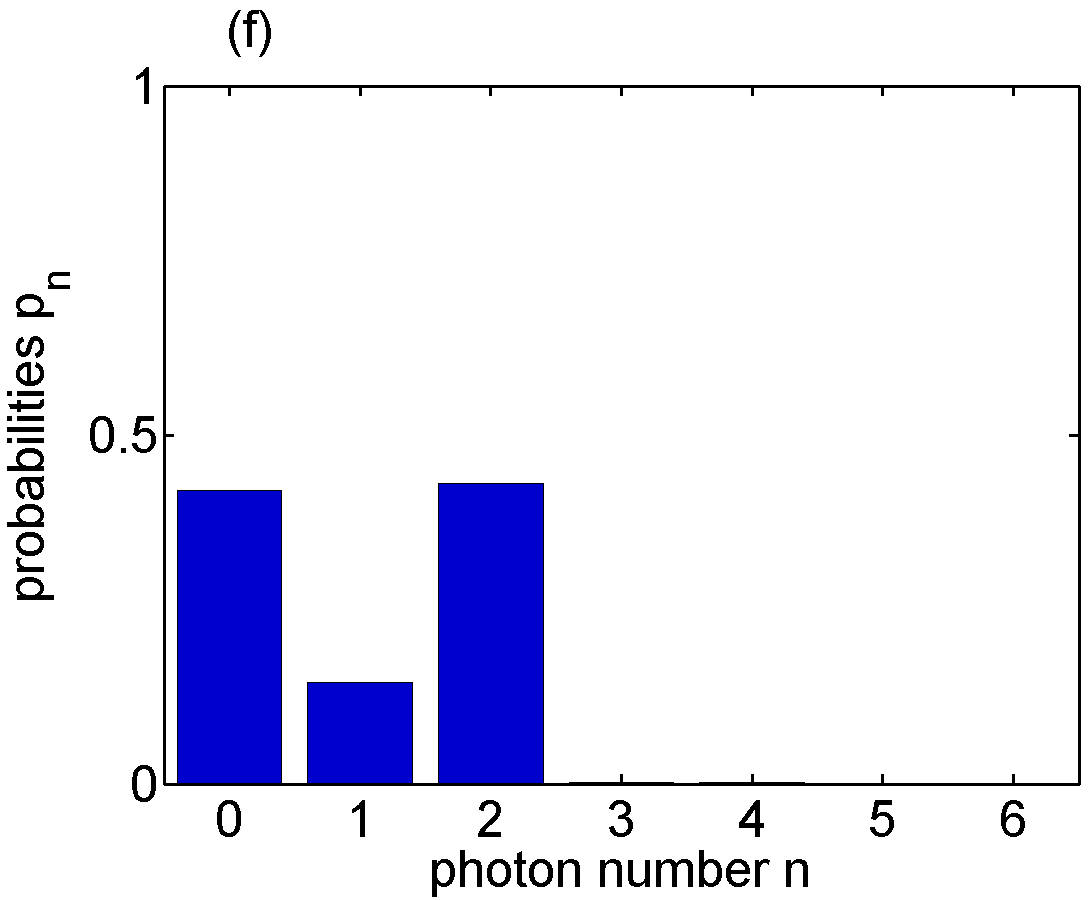
Figure 10: (Color online) Model 1 with two-photon dissipation: Same as in Fig. 6, but for different initial states: (a,b) coherent state $|\alpha=3/4\rangle$, with $p_{0}\approx p_{1}\approx p_{2}$, (c,d) coherent state $|\alpha=2\rangle$, with $p_{1}>p_{0}\approx p_{2}$, and (e,f) the cat state $|\alpha=2,\phi=\pi/4\rangle$, with $p_{1}<p_{0}\approx p_{2}$.

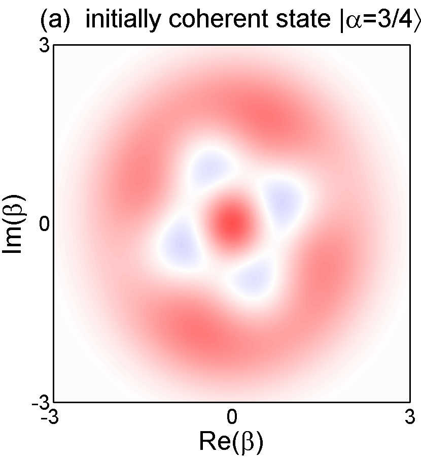
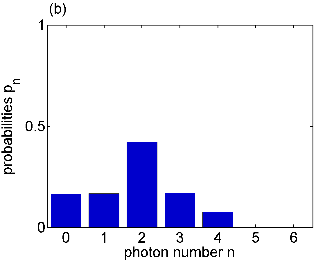
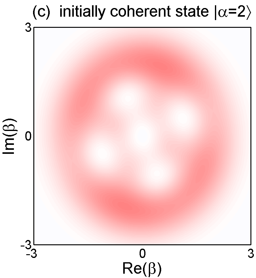
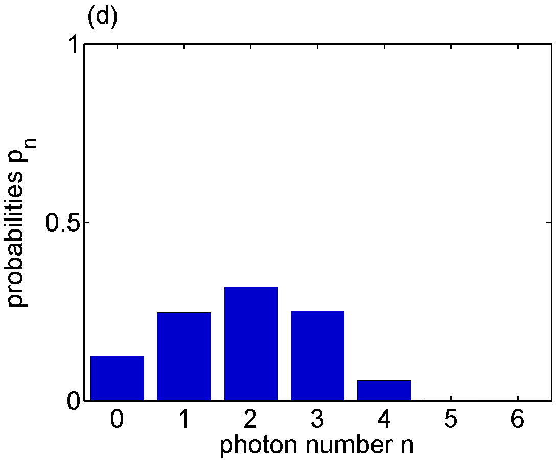
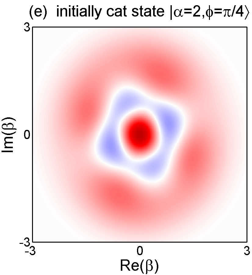
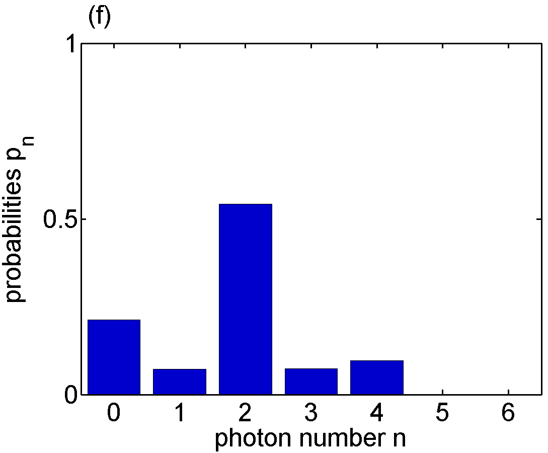
Figure 11: (Color online) Model 2 with two-photon dissipation: Same as in Fig. 10, but for the steady-state solutions $\hat{\rho}^{13}_{{\rm ss}}$ of the master equation (26) with the Hamiltonian $\hat{H}_{13}$, given by Eq. (17).

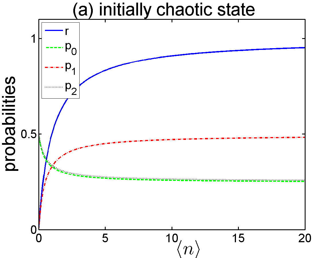
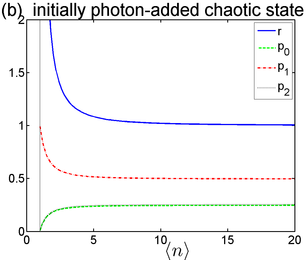
Figure 12: (Color online) Model 1 with two-photon dissipation: Photon-number probabilities $p_{n}={\langle n|\,}\hat{\rho}^{02}_{{\rm ss}}{\,|n\rangle}$ and ratio $r$ versus mean photon number ${\langle n\rangle}$ for different initial cavity fields: (a) chaotic state $\hat{\rho}_{{\rm ch}}$ and (b) single-photon-added chaotic state $\hat{\rho}_{{}_{\rm AT}}$.

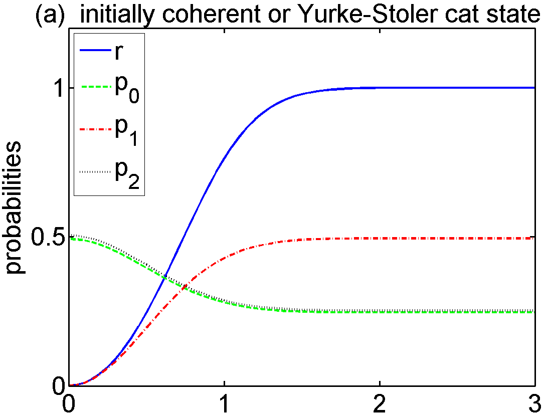
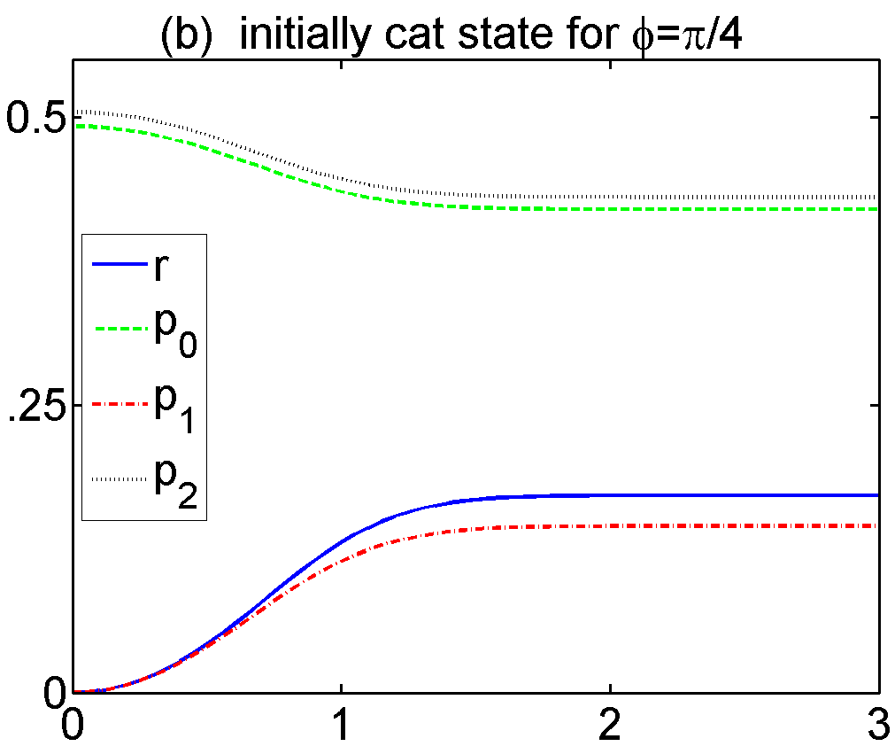
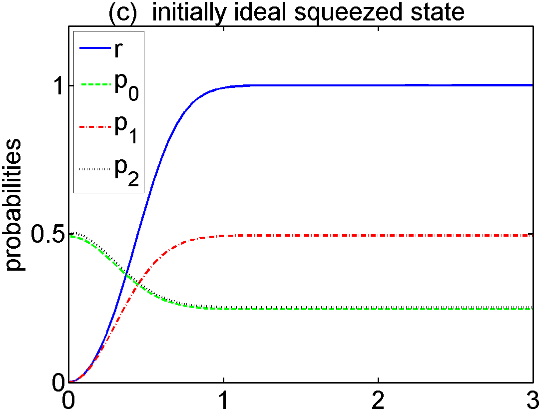
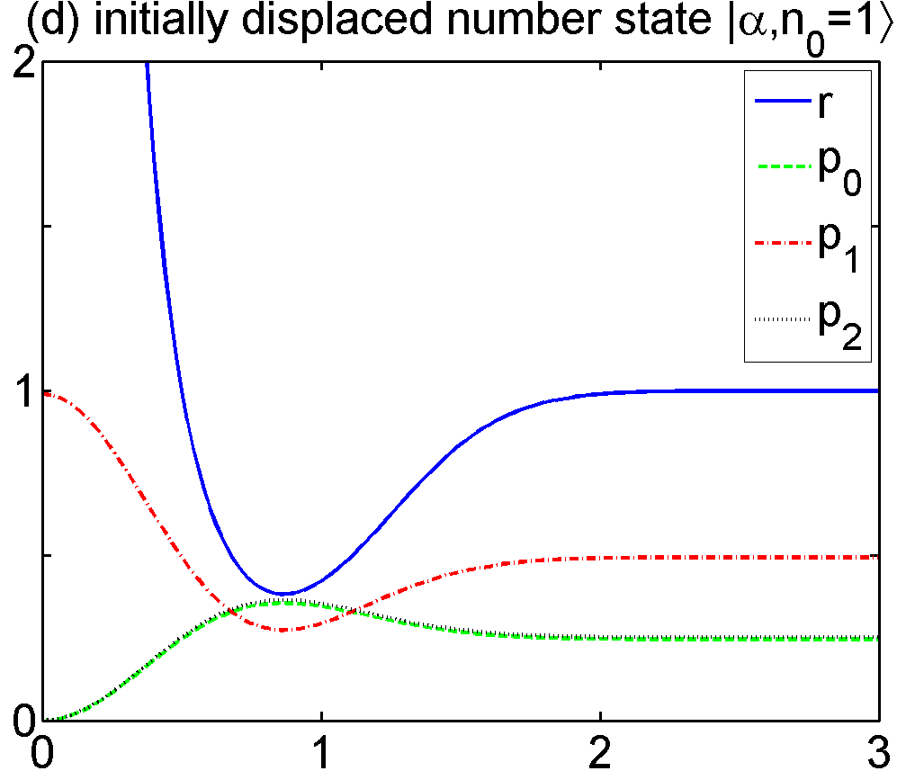
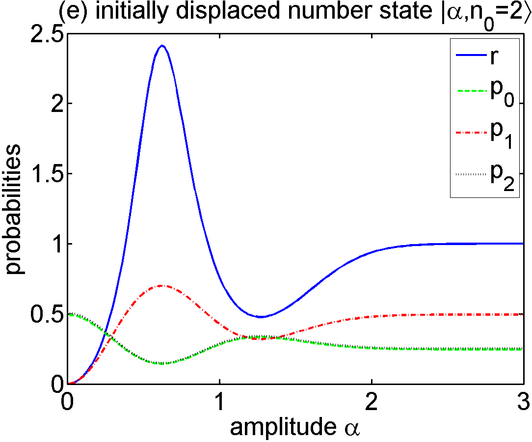
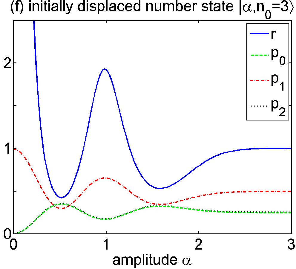
Figure 13: (Color online) Model 1 with two-photon dissipation: The figure shows how the steady state $\hat{\rho}^{02}_{{\rm ss}}$ in the engineered photon blockade depends on initial cavity field $|\psi_{0}\rangle$. The photon-number probabilities $p_{n}={\langle n|\,}\hat{\rho}^{02}_{{\rm ss}}{\,|n\rangle}$ (for $n=0,1,2$) and the ratio $r=p_{{\rm odd}}(|\psi_{0}\rangle)/p_{{\rm even}}(\psi_{0}\rangle)$ versus real amplitude $\alpha$ for various initial states $|\psi_{0}\rangle$: (a) coherent state $|\alpha\rangle$ or, equivalently, the Yurke-Stoler cat state $|\alpha_{{}_{\rm YS}}\rangle=|\alpha,\phi=\pi/2\rangle$, (b) the cat state $|\alpha,\phi=\pi/4\rangle$, and (c) the ideal squeezed state $|\alpha,\xi=1/2\rangle$, and (d,e,f) the displaced number states $|\alpha,n_{0}\rangle$ with $n_{0}=1,2,3$. The steady-state solutions $\hat{\rho}^{02}_{{\rm ss}}$ of the master equation (26) for the Hamiltonian $\hat{H}_{02}$ are obtained assuming $\delta=\epsilon/\chi=1/6$ and $\delta^{\prime}=\gamma/\epsilon=1/25$.

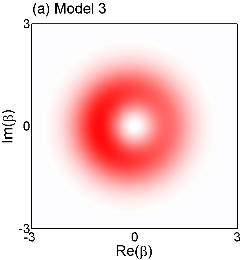
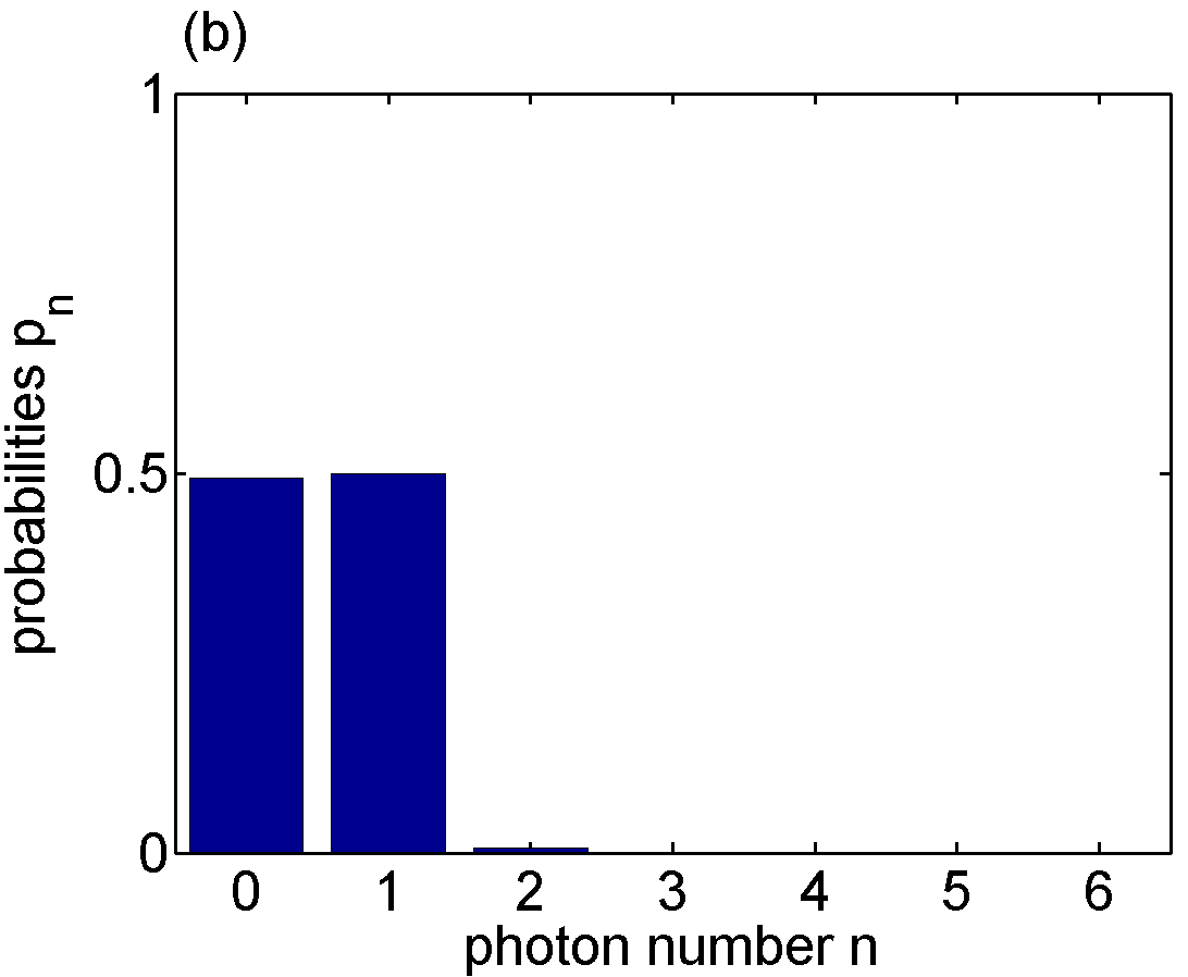
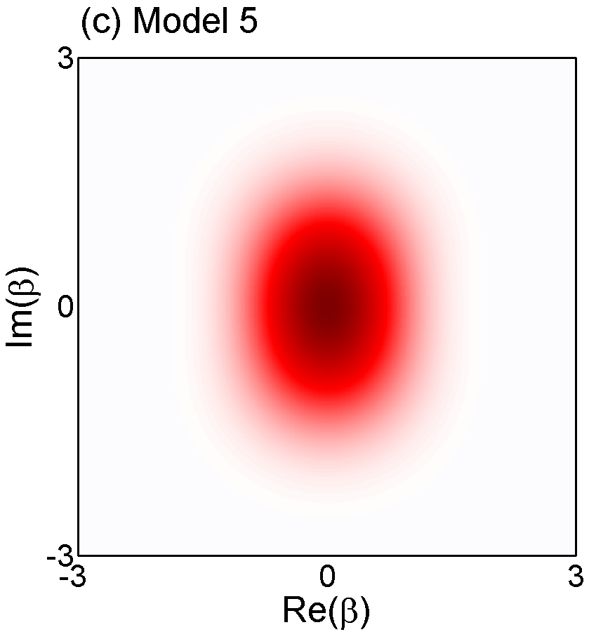
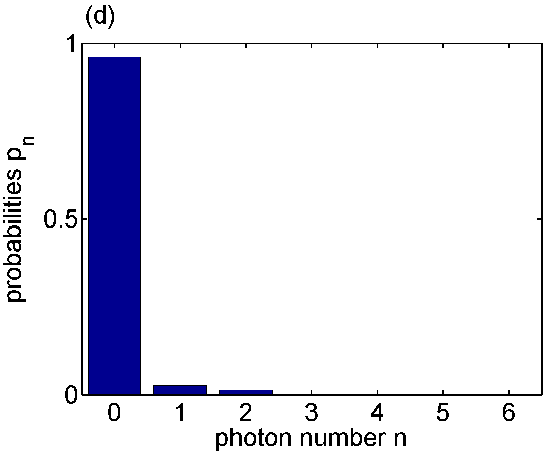
Figure 14: (Color online) Models 3 in panels (a,b) and 5 in (c,d) with single-photon dissipation for any initial states: Wigner functions $W(\beta)$ and photon-number probabilities $p_{n}$ for the steady-state solutions of the master equation (27) with $\gamma_{2}=\gamma_{\perp}=0$ for: (a,b) the single-photon driven Hamiltonian $\hat{H}_{\rm usual}$, given by Eq. (20), and (c,d) the two-photon driven Hamiltonian $\hat{H}_{01}$, given by Eq. (17) with $k=0,l=1$. We set $\delta=\epsilon/\chi=1/6$ and $\gamma_{1}/\epsilon=1/25$. Model 3 corresponds to the standard description of photon blockade. It is worth noting that the same solutions, as shown in panels (a,b), can be obtained for the two-photon absorption master equation, given by Eq. (26) with $\delta^{\prime}=\gamma/\epsilon=1/25$. This case is referred to as Model 3’ in Table I.

V Photon blockade for specific initial fields

Here we analyze how the engineered photon blockade depends on some typical classical and nonclassical initial states of the cavity field.

For a coherent state (CS) $|\alpha\rangle$, we have

$$p_{{\rm even}}(|\alpha\rangle) = \frac{1}{2}[1+\exp(-2|\alpha|^{2})],$$

$$p_{{\rm odd}}(|\alpha\rangle) = \frac{1}{2}[1-\exp(-2|\alpha|^{2})],$$ (40)

so their ratio is $r=\tanh(|\alpha|^{2})$. In the limiting cases, one observes that

$$\lim_{{\langle n\rangle}\rightarrow 0}p_{{\rm even}}(\hat{\rho}_{0}) = 1,\quad\lim_{{\langle n\rangle}\rightarrow 0}p_{{\rm odd}}(\hat{\rho}_{0})=0,$$ (41)

$$\lim_{{\langle n\rangle}\rightarrow\infty}p_{{\rm even}}(\hat{\rho}_{0}) = \lim_{{\langle n\rangle}\rightarrow\infty}p_{{\rm odd}}(\hat{\rho}_{0})=\frac{1}{2},$$ (42)

where $\hat{\rho}_{0}=|\alpha\rangle\langle\alpha|$ and the intensity is given by ${\langle n\rangle}=|\alpha|^{2}$. A few illustrative examples of phase-space and photon-number distributions for the steady-state solutions, for initial coherent states, are shown in Fig. 10 for Model 1 and in Fig. 11 for Model 2.

For the chaotic (or thermal) state of the cavity field,

$$\hat{\rho}_{{\rm ch}}=(1-q)\sum_{n=0}^{\infty}q^{n}|n\rangle\langle n|,$$ (43)

where $\langle n\rangle=q/(1-q)$ is the mean photon number, one can find that

$$p_{{\rm even}}(\hat{\rho}_{{\rm ch}}) = \frac{1}{1+q}=\frac{1+\langle n\rangle}{1+2\langle n\rangle},$$

$$p_{{\rm odd}}(\hat{\rho}_{{\rm ch}}) = \frac{q}{1+q}=\frac{\langle n\rangle}{1+2\langle n\rangle},$$ (44)

so $r(\hat{\rho}_{{\rm ch}})=q=\langle n\rangle/(\langle n\rangle+1)$. In the limiting cases of the intensity ${\langle n\rangle}$, one can see that the relations Eqs. (41) and (42) hold also for $\hat{\rho}_{0}=\hat{\rho}_{{\rm ch}}$, as for coherent states. Figure 12(a) shows how the photon-number probabilities $p_{n}$ of the steady-state solutions $\hat{\rho}_{{\rm ss}}(\hat{\rho}_{0})$ depend on the mean photon number ${\langle n\rangle}$ of the initial chaotic state $\hat{\rho}_{0}=\hat{\rho}_{{\rm ch}}$.

Now we analyze a few examples of nonclassical initial states.

The single-photon-added chaotic state, introduced by Agarwal and Tara Agarwal92 , can be defined as follows

$$\hat{\rho}_{{}_{\rm AT}}={\cal N}\hat{a}^{\dagger}\hat{\rho}_{{\rm ch}}\hat{a}={\cal N}\sum_{n=1}^{\infty}nq^{n}|n\rangle\langle n|,$$ (45)

where $\hat{\rho}_{{\rm ch}}$ is the chaotic state, given by Eq. (43), $\hat{a}$ ($\hat{a}^{\dagger}$) is the annihilation (creation) operator of the field, and ${\cal N}=(1-q)^{2}/q$ is the normalization constant. The mean photon number for $\hat{\rho}_{{}_{\rm AT}}$ is $\langle n\rangle=(1+q)/(1-q)$. It is interesting to note that this infinite-dimensional state is nonclassical although diagonal in the photon-number basis. We find that

$$p_{{\rm even}}(\hat{\rho}_{{}_{\rm AT}}) = \frac{2q}{(1+q)^{2}}=\frac{1}{2}(1-{\langle n\rangle}^{-2}),$$

$$p_{{\rm odd}}(\hat{\rho}_{{}_{\rm AT}}) = \frac{1+q^{2}}{(1+q)^{2}}=\frac{1}{2}(1+{\langle n\rangle}^{-2}),$$ (46)

so $r(\hat{\rho}_{{}_{\rm AT}})=(1+q^{2})/(2q)=(1+{\langle n\rangle}^{2})/(1-{\langle n\rangle}^{2})$. In the limit of large number of photons, ${\langle n\rangle}\rightarrow\infty$, again the relation, given by Eq. (42), hold as for chaotic states. However, in the limit of small number of photons, we have

$$\lim_{{\langle n\rangle}\rightarrow 1}p_{{\rm even}}(\hat{\rho}_{{}_{\rm AT}}) = 0,\quad\lim_{{\langle n\rangle}\rightarrow 1}p_{{\rm odd}}(\hat{\rho}_{{}_{\rm AT}})=1,$$ (47)

which is the opposite case to the chaotic state, as given by Eq. (41). Note that ${\langle n\rangle}\geq 1$, because only then $p_{{\rm odd}}(\hat{\rho}_{{}_{\rm AT}})\leq 1$. Figure 12(b) shows how the photon-number probabilities $p_{n}={\langle n|\,}\hat{\rho}_{{\rm ss}}(\hat{\rho}_{0}){\,|n\rangle}$ depend on the mean photon number ${\langle n\rangle}$ of the initial single-photon-added chaotic state $\hat{\rho}_{0}=\hat{\rho}_{{\rm AT}}$. This dependence is fundamentally different from that shown in Fig. 12(a) for the initial chaotic state.

Let us also analyze a prototype of Schrödinger’s cat states given as a macroscopically distinct superposition of two coherent states, e.g.,

$$|\alpha,\phi\rangle={\cal{\cal N}}[|\alpha\rangle+\exp(i\phi)|-\alpha\rangle]$$ (48)

with the normalization ${\cal{\cal N}}=\{2[1+\cos\phi\exp(-2|\alpha|^{2})]\}^{-1/2}$ assuming a complex amplitude $\alpha.$ One can find that

$$p_{{\rm even}}(|\alpha,\phi\rangle) = \cos^{2}\Big{(}\frac{\phi}{2}\Big{)}\frac{1+\exp(-2|\alpha|^{2})}{1+\cos\phi\exp(-2|\alpha|^{2})},$$

$$p_{{\rm odd}}(|\alpha,\phi\rangle) = \sin^{2}\Big{(}\frac{\phi}{2}\Big{)}\frac{1-\exp(-2|\alpha|^{2})}{1+\cos\phi\exp(-2|\alpha|^{2})},$$

$$r = \tan^{2}(\phi/2)\tanh|\alpha|^{2}.$$ (49)

For special choices of $\phi=0,\pi/2,\pi$, the state $|\alpha,\phi\rangle$ reduces to the renowned cat states. These include the even CS

$$|\alpha_{+}\rangle\equiv|\alpha,\phi=0\rangle=\frac{1}{\sqrt{\cosh|\alpha|^{2}}}\sum_{n=0}^{\infty}\frac{\alpha^{2n}}{\sqrt{(2n)!}}|2n\rangle,$$ (50)

the Yurke-Stoler cat state $|\alpha_{{}_{\rm YS}}\rangle\equiv|\alpha,\phi=\pi/2\rangle$ Yurke86 , and the odd CS

$$|\alpha_{-}\rangle\equiv|\alpha,\phi=\pi\rangle=\frac{1}{\sqrt{\sinh|\alpha|^{2}}}\sum_{n=0}^{\infty}\frac{\alpha^{2n+1}}{\sqrt{(2n+1)!}}|2n+1\rangle.$$ (51)

Clearly, $p_{{\rm even}}(|\alpha_{+}\rangle)=1$ and $p_{{\rm odd}}(|\alpha_{-}\rangle)=1$ for any $\alpha$, this is in contrast to the states $|\alpha,\phi\rangle$ for other angles $\phi$. Equation (49) for the Yurke-Stoler cat state $|\alpha_{{}_{\rm YS}}\rangle$ implies that

$$p_{{\rm even}}(|\alpha_{{}_{\rm YS}}\rangle)=p_{{\rm even}}(|\alpha\rangle).$$ (52)

Thus, the formulas given by Eqs. (40)–(42), hold for the state $|\alpha_{{}_{\rm YS}}\rangle$ too. A few examples of the Wigner functions and photon-number probabilities for the steady-state solutions, obtained for initial cat states, are shown in Figs. 10(e,f) and 13(a,b) for Model 1 and in Fig. 11(e,f) for Model 2.

In Fig. 13, we also analyze the engineered photon blockade for squeezed and displaced-number initial states. The ideal squeezed states (also known as the two-photon coherent states) are defined as

$$|\alpha,\xi\rangle = \hat{D}(\alpha)\hat{S}(\xi)|0\rangle,$$ (53)

which are given in terms of the squeeze operator $\hat{S}(\xi)=\exp[\tfrac{1}{2}\xi^{*}a^{2}-\tfrac{1}{2}\xi(a^{\dagger})^{2}],$ where $\xi$ is the complex squeezing parameter, and the displacement operator $\hat{D}(\alpha)=\exp(\alpha\hat{a}^{\dagger}-\alpha^{*}\hat{a})$ with a complex amplitude $\alpha$. The displaced-number states are defined by

$$|\alpha,n_{0}\rangle=\hat{D}(\alpha)|n_{0}\rangle,$$ (54)

which become a coherent state $|\alpha\rangle$ in a special case of $n_{0}=0$. The photon-number expansions of these are given in Appendix B. These are useful to find the steady-state solutions, given by Eq. (33). Except for some special cases, including squeezed vacuum $|\alpha=0,\xi\rangle$ and coherent state $|\alpha,n_{0}=0\rangle$, the formulas for the probabilities $p_{{\rm even}}$ and $p_{{\rm odd}}$ are not compact, thus we present only our numerical results in Fig. 13.

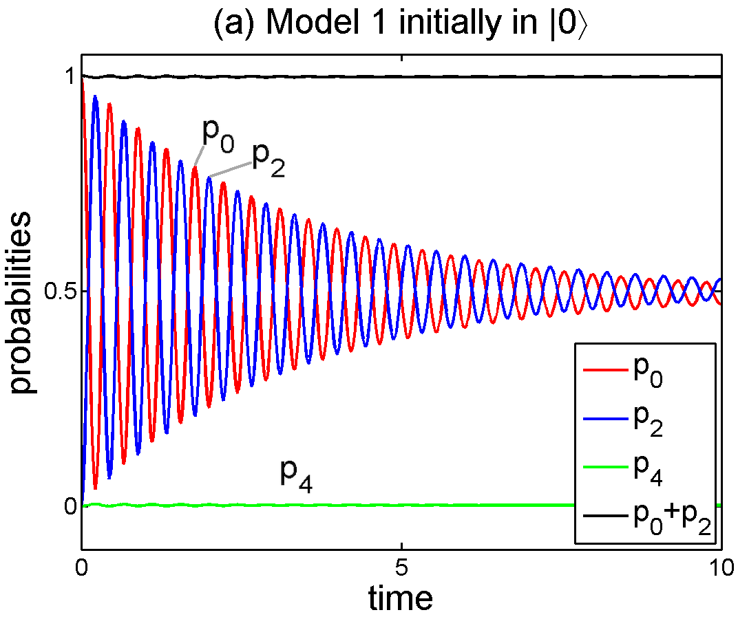
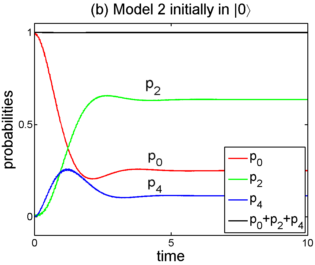
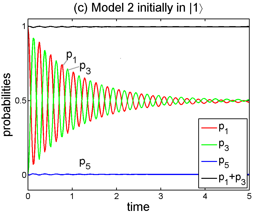
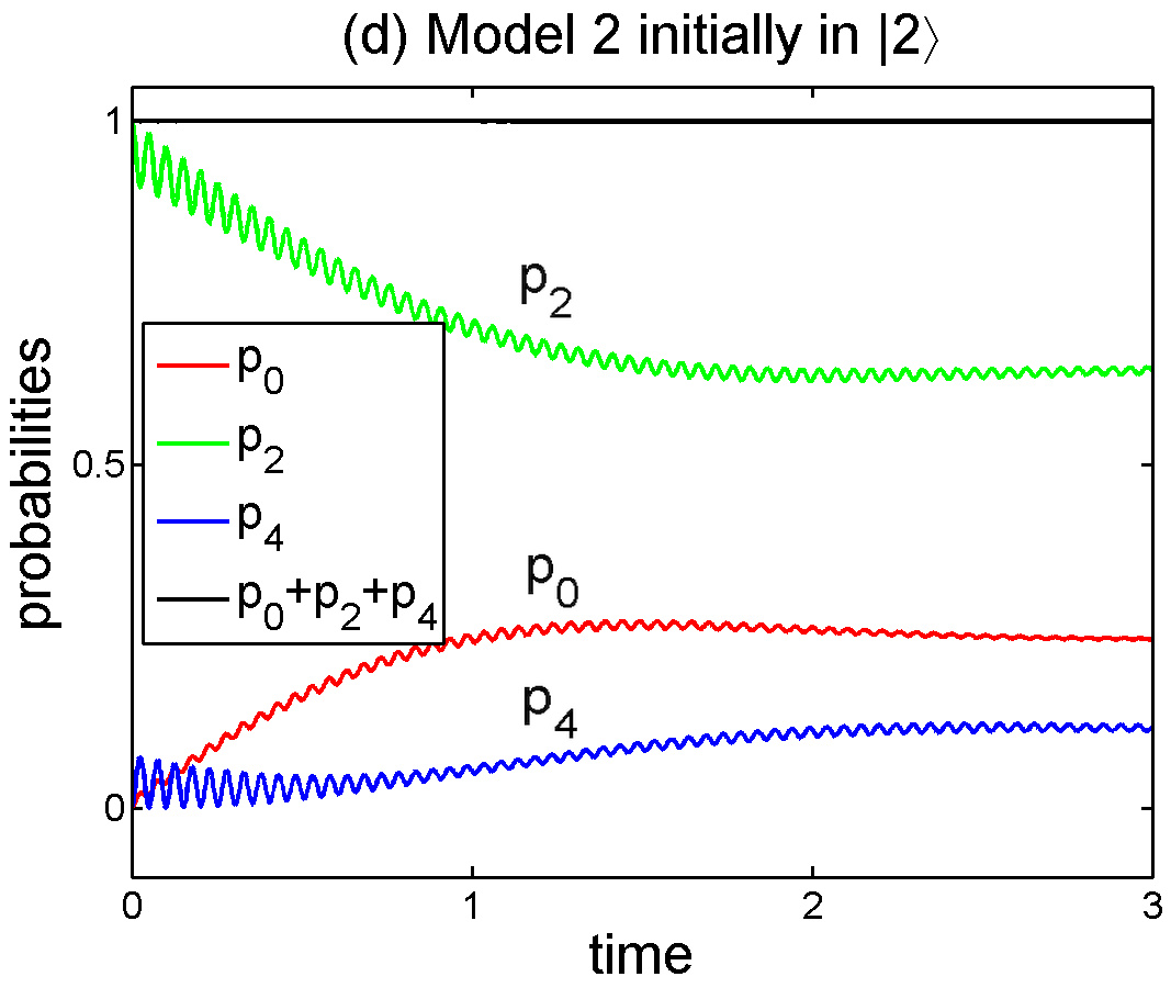
Figure 15: (Color online) Models 1(a) and 2 (b,c,d): Dissipative evolutions of the photon-number probabilities $p_{n}(t)$ and the photon-blockade fidelities $F(t)=\sum_{n}p_{n}(t)$ for several initial Fock states ${\,|m\rangle}$ (as indicated in the panel titles) assuming $\delta=\epsilon/\chi=1/6$, $\delta^{\prime}=\gamma/\epsilon=1/25$, and $\epsilon=5$. The decay of Rabi-type oscillations is clearly seen. Panels (a) and (b,c,d) should be compared with Figs. 1(a) and 2(a,b,c) demonstrating the corresponding dissipation-free evolutions in Models 1 and 2, respectively. It is seen that the decaying states rapidly approach the steady states shown in Figs. 6 and 7.

VI Conclusions

We studied photon blockade (also known as optical-state truncation) of an optical or microwave light in a Kerr nonlinear cavity parametrically driven by a two-photon process. The Kerr nonlinear cavity can be effectively implemented by a standard linear cavity with a tunable two-level system within the Jaynes-Cummings model in the dispersive limit. We have also assumed that the nonlinear system interacts with a nonlinear reservoir, where two-photon absorption is dominant. We have shown in Sec. II how to observe various types of photon blockade effects (as summarized in Table I) by properly tuning the frequencies of the driving field and the two-level system.

Our approach is partially motivated by the observation that two-photon loss mechanisms often accompany a Kerr nonlinearity Yurke06 . Moreover, quantum reservoirs are a powerful resource for quantum state engineering (see, e.g., Refs. Gilles93 ; Kim93 ; Gilles94 ; Guerra97 ; Ispasoiu00 ; Jakob01 ; Klimov03 ; Buks06 ; Yurke06 ; Karasik08 ; Kowalewska10 ; Boissonneault12 ; Everitt13 ; Kumar10 ; Gevorkyan10 ; Mogilevtsev13 ; Leghtas13 ; Reiter13 ; Arenz13 ; Mirrahimi14 ; Lu14 ). In particular, the circuit described in Ref. Kumar10 for the implementation of nondemolition measurement using the Kerr effect seems to be readily applicable not only for generating Schrödinger cat states Everitt13 , but also for implementing our generalized photon blockade via two-photon dissipation. Anyway, such an implementation would require a detailed analysis, which is not presented here.

The conditions to observe photon blockade are the following: (i) the system must exhibit nonlinearity which is much stronger than the strength of the drive, and (ii) dissipation is weaker than the drive. (Actually, the second condition can be relaxed, as seen in Fig. 8.) Thus, in particular, photon blockade can also be observed even without damping at all. The system evolution is limited to a few number states, which are determined by the choice of initial states and the values of the tuning parameters $k,l$ in the Hamiltonian $H_{kl}$. This effect is referred to as nonstationary (or time-dependent) photon blockade. As discussed in Sec. III and shown in Figs. 1 and 3, Rabi-type oscillations can occur between some number states, while practically no evolution can be observed for other states. If the system is damped, then these Rabi-type oscillations decrease in amplitude, and completely disappear for longer times, as shown in Fig. 15 both for Models 1 and 2. The evolutions of these driven and dissipative nonlinear systems generate nonclassical optically truncated steady states corresponding to stationary (or steady-state) photon blockade. The phase-space and photon-number distributions of these states are shown in Figs. 6–14.

It is well known that a typical steady-state photon blockade does not depend on the initial state of a Kerr nonlinear system if it is driven by a single-photon process and coupled to a standard reservoir, where only a single-photon absorption is allowed, as illustrated in Figs. 14(a,b) and listed in Table I.

In contrast, we have shown that the engineered photon blockade can depend on the system initial state (see Table I for comparison of various photon blockade effects). This state dependence occurs in a Kerr nonlinear system driven by a two-photon process and dissipating via an engineered quantum reservoir, where only two-photon absorption is allowed. These two-photon driving and dissipation processes result in two completely independent evolutions of the superpositions of Fock states with either even or odd numbers of photons. This can be interpreted as two different evolution-dissipation channels for even and odd-number states. So, in particular, these states evolve into two different steady states in the time limit. As the two processes affect only every second state in the Fock basis and there is no mixing between the photon numbers of different parity, we can describe their evolutions in two independent Hilbert spaces. If the initial state is a superposition of photon-number states of different parity, then its steady state is a weighted sum of the steady states achieved independently in the even- and odd-number Hilbert spaces. The weights in this mixture depend on the photon-number statistics of the initial states, although in a limited way, as they depend solely on the ratio of the probabilities of measuring the odd and even numbers of initial-state photons.

The above results imply that photon blockade phenomena do not depend on the initial states for various other models listed in Table I, for example, if a two-photon driving is combined with a single-photon dissipation or, vice versa, if a single-photon driving is accompanied by a two-photon dissipation. This is because, one of these processes (i.e., the driving or dissipation) mixes the evolutions of the Hilbert spaces with even and odd photon numbers.

To confirm these predictions we found approximate analytical steady-state solutions, given in Eqs. (30)–(33), of the master equation, given by Eq. (26). We also obtained precise numerical solutions in a 100-dimensional Hilbert space, as shown in all our plots. We found a very good agreement between these numerical and approximate analytical solutions. Moreover, we observed that they depend solely on the ratios between the driving field strength $\epsilon$, the Kerr nonlinear coupling $\chi$, and the damping constant $\gamma$; i.e., $\delta=\epsilon/\chi$ and $\delta^{\prime}=\gamma/\epsilon$. So, the absolute values of $\epsilon$, $\chi$, and $\gamma$ are irrelevant.

We analyzed a few examples of standard infinite-dimensional quantum optical states including coherent, squeezed, displaced number, chaotic, photon-added chaotic and Schrödinger’s cat states to show how the photon-number statistics of an initial state influences its steady state. As an illustration of our results, the Wigner functions and photon-number probabilities for the steady states are shown in Figs. 6–14. We note that some of these states have nonnegative Wigner functions (i.e., without regions marked in blue). Nevertheless all them are nonclassical; i.e., their Glauber-Sudarshan $P$ function is negative in some regions of phase space.

We hope that our proposal of state-dependent photon blockade via a two-photon absorbing reservoir is another convincing example demonstrating how to harness quantum-reservoir engineering for quantum technology.

Appendix A Approximate steady-state solutions

Here we give approximate formulas for the coefficients $a,b,...,r$ occurring in the steady-state solutions, given by Eqs. (30) and (32), as obtained by expanding our precise but lengthy solutions (thus, not presented here) in power series of $\delta=\epsilon/\chi\ll 1$ and $\delta^{\prime}=\gamma/\epsilon\ll 1$ and keeping terms only up to $\delta^{2}$, $\delta^{\prime 2}$, and $\delta\delta^{\prime}$.

The coefficients in Eq. (30), where the initial state was assumed to have an even number of photons, for the Hamiltonian $\hat{H}_{02}$ (Model 1) are given by

$$p=\tfrac{1}{2}-\tfrac{9}{32}\delta^{2}+\tfrac{1}{8}\delta^{\prime 2},\quad q=1-p-r,\quad r= \tfrac{3}{32}\delta^{2},$$ (55)

for the diagonal terms of $\hat{\rho}^{{\rm even}}_{{\rm ss}}$ and

$$a=-\tfrac{3}{8}\sqrt{2}\delta,\quad b=\tfrac{1}{4}\sqrt{2}\delta^{\prime},\quad c=\tfrac{5}{64}\sqrt{6}\delta^{2},$$

$$d=-\tfrac{1}{16}\sqrt{6}\delta\delta^{\prime},\quad e=-\tfrac{1}{8}\sqrt{3}\delta,\quad f=0$$ (56)

for its off-diagonal terms, while the coefficients for the Hamiltonian $\hat{H}_{13}$ (Model 2) are found to be

$$p=\tfrac{25}{32}-\tfrac{107}{512}\delta^{2},\;\;\;q=\tfrac{3}{16}+\tfrac{15}{128}\delta^{2},\quad s=\tfrac{5}{768}\delta^{2},$$ (57)

and $r=1-p-q-s,$ for the diagonal terms, and

$$a= \tfrac{19}{128}\sqrt{2}\delta,\quad b= \tfrac{3}{32}\sqrt{2}\delta,$$

$$c= -\tfrac{37}{4608}\sqrt{6}\delta^{2},\quad d= \tfrac{1}{16}\sqrt{6}-\tfrac{49}{768}\sqrt{6}\delta^{2},$$

$$e= -\tfrac{5}{64}\sqrt{3}\delta,\quad f= \tfrac{1}{32}\sqrt{3}\delta$$ (58)

for the off-diagonal terms. For simplicity, we set $\delta=\delta^{\prime}$ in Eqs. (57) and (58).

The coefficients in Eq. (32), where the initial state was assumed to have an odd number of photons, for the Hamiltonian $\hat{H}_{02}$ (Model 1) read

$$p = 1-\frac{6\epsilon^{2}}{M}\approx 1-\frac{3}{8}\delta^{2}\approx 1,$$

$$a = -4\sqrt{6}\frac{\chi\epsilon}{M}\approx-\frac{\sqrt{6}}{4}\delta,$$

$$b = 3\sqrt{6}\frac{\epsilon\gamma}{M}\approx\frac{3}{16}\sqrt{6}\delta\delta^{\prime}\approx 0,$$ (59)

where $M=16\chi^{2}+12\epsilon^{2}+9\gamma^{2}$, while these coefficients for the Hamiltonian $\hat{H}_{13}$ (Model 2) are given by

$$p=1-\frac{2\epsilon^{2}}{M}\approx\frac{1}{2},\quad a=0,\quad b=\sqrt{6}\frac{\epsilon\gamma}{M}\approx\frac{\sqrt{6}}{4}\delta^{\prime},$$ (60)

where $M=4\epsilon^{2}+3\gamma^{2}$.

Appendix B Some photon-number expansions

Here we give some formulas useful for the calculation of the probabilities $p_{{\rm even}}(\hat{\rho}_{0})$ and $p_{{\rm odd}}(\hat{\rho}_{0})$, and their ratio $r$ for the squeezed and displaced-number states $\hat{\rho}_{0}$, shown in Fig. 13.

The photon-number expansion of the ideal squeezed states, defined by Eq. (53), is given by

$$|\alpha,\xi\rangle=\sum_{n}\langle n|\alpha,\xi\rangle|n\rangle\equiv\sum_{n}c_{n}|n\rangle,$$ (61)

where

$$c_{n}=\left(\frac{x}{2}\right)^{n/2}\frac{H_{n}(y)\exp(-z/2)}{\sqrt{n!}\cosh(|\xi|)},$$

in terms of the Hermite polynomials $H_{n}(y)$, $x=\tanh(|\xi|)\exp(i{\rm Arg}\xi),$ $y=(2x)^{-1/2}(\alpha+\alpha^{*}x),$ and $z=|\alpha|^{2}+(\alpha^{*})^{2}x$.

The photon-number expansion of the displaced number states, defined by Eq. (54), is given by Oliveira90 ; Tanas96 :

$$|\alpha,n_{0}\rangle = \sum_{n}b_{n}\exp[i(n-n_{0})\,{\rm Arg}\alpha]|n\rangle,$$ (62)

where the real amplitudes $b_{n}$ are

$$b_{n}=\langle n|\hat{D}(|\alpha|)|n_{0}\rangle\hskip 128.0374pt$$

$$=C\,\sqrt{\frac{n_{-}!}{n_{+}!}}(-1)^{n_{+}-n}|\alpha|^{n_{+}-n_{-}}L_{n_{-}}^{(n_{+}-n_{-})}(|\alpha|^{2}),$$ (63)

where $L_{n}^{(m)}(x)$ are the associated Laguerre polynomials, $C=\exp\left(-\frac{1}{2}|\alpha|^{2}\right)$, $n_{-}=\min\{n,n_{0}\},$ and $n_{+}=\max\{n,n_{0}\}=n+n_{0}-n_{-}.$

References

- (1) Z. L. Xiang, S. Ashhab, J. Q. You, and F. Nori, Hybrid quantum circuits: Superconducting circuits interacting with other quantum systems, Rev. Mod. Phys. 85, 623 (2013).
- (2) H. D. Simaan and R. Loudon, Off-diagonal density matrix for single-beam two-photon absorbed light, J. Phys. A 11, 435 (1978).
- (3) L. Gilles and P. L. Knight, Two-photon absorption and nonclassical states of light, Phys. Rev. A 48, 1582 (1993).
- (4) L. Gilles, B.M. Garraway, and P. L. Knight, Generation of nonclassical light by dissipative two-photon processes, Phys. Rev. A 49, 2785 (1994).
- (5) E. S. Guerra, B. M. Garraway, and P. L. Knight, Two-photon parametric pumping versus two-photon absorption: A quantum jump approach, Phys. Rev. A 55, 3842 (1997).
- (6) V. V. Dodonov and S. S. Mizrahi, Competition between one- and two-photon absorption processes, J. Phys. A 30, 2915 (1997).
- (7) M. J. Everitt, T. P. Spiller, G. J. Milburn, R. D. Wilson, and A. M. Zagoskin, Cool for cats, e-print arXiv:1212.4795.
- (8) R. G. Ispasoiu, T. Goodson III, Photon-number squeezing by two-photon absorption in an organic polymer, Opt. Commun. 178, 371 (2000).
- (9) A. B. Klimov and J. L. Romero, An algebraic solution of Lindblad-type master equations, J. Opt. B: Quantum Semicalssical Opt.5, S316 (2003).
- (10) E. Buks and B. Yurke, Dephasing due to intermode coupling in superconducting stripline resonators, Phys. Rev. A 73, 023815 (2006).
- (11) B. Yurke and E. Buks, Performance of cavity-parametric amplifiers, employing Kerr nonlinearites, in the presence of two-photon loss, J. Lightwave Tech. 24, 5054 (2006).
- (12) R. I. Karasik, K. P. Marzlin, B. C. Sanders, and K. B. Whaley, Criteria for dynamically stable decoherence-free subspaces and incoherently generated coherences, Phys. Rev. A 77, 052301 (2008).
- (13) M. Boissonneault, A. C. Doherty, F. R. Ong, P. Bertet, D. Vion, D. Esteve, and A. Blais, Back-action of a driven nonlinear resonator on a superconducting qubit, Phys. Rev. A 85, 022305 (2012).
- (14) A. Voje, A. Croy, and A. Isacsson, Multi-phonon relaxation and generation of quantum states in a nonlinear mechanical oscillator, New J. Phys. 15, 053041 (2013).
- (15) V. V. Albert and L. Jiang, Symmetries and conserved quantities in Lindblad master equations, Phys. Rev. A 89, 022118 (2014).
- (16) S. Kumar and D. P. DiVincenzo, Exploiting Kerr cross nonlinearity in circuit quantum electrodynamics for nondemolition measurements, Phys. Rev. B 82, 014512 (2010).
- (17) S. T. Gevorkyan and M. S. Gevorkyan, Three-Component Superposition States of Light in a Dissipative Medium, Opt. Spectr. 109, 126 (2010).
- (18) D. Mogilevtsev, A. Mikhalychev, V. S. Shchesnovich, and N. Korolkova, Nonlinear dissipation can combat linear loss, Phys. Rev. A 87, 063847 (2013).
- (19) Z. Leghtas, U. Vool, S. Shankar, M. Hatridge, S. M. Girvin, M. H. Devoret, and M. Mirrahimi, Stabilizing a Bell state of two superconducting qubits by dissipation engineering, Phys. Rev. A 88, 023849 (2013).
- (20) F. Reiter, L. Tornberg, G. Johansson, and A. S. Sorensen, Steady-state entanglement of two superconducting qubits engineered by dissipation, Phys. Rev. A 88, 032317 (2013).
- (21) C. Arenz, C. Cormick, D. Vitali, and G. Morigi, Generation of two-mode entangled states by quantum reservoir engineering, J. Phys. B 46, 224001 (2013).
- (22) M. Mirrahimi, Z. Leghtas, V. V. Albert, S. Touzard, R. J. Schoelkopf, L. Jiang, and M. H. Devoret, Dynamically protected cat-qubits: a new paradigm for universal quantum computation, New J. Phys. 16, 045014 (2014).
- (23) X.Y. Lü, J. Q. Liao, L. Tian, and F. Nori, Steady-state Mechanical Squeezing in an Optomechanical System via Duffing Nonlinearity, e-print arXiv:1403.0049.
- (24) Y. X. Liu, A. Miranowicz, Y. B. Gao, J. Bajer, C. P. Sun, and F. Nori, Qubit-induced phonon blockade as a signature of quantum behavior in nanomechanical resonators, Phys. Rev. A82, 032101 (2010).
- (25) Y.X. Liu, X.W. Xu, A. Miranowicz, and F. Nori, From blockade to transparency: Controllable photon transmission through a circuit QED system, Phys. Rev. A89, 043818 (2014),
- (26) N. Didier, S. Pugnetti, Y. M. Blanter, and R. Fazio, Detecting phonon blockade with photons, Phys. Rev. B84, 054503 (2011).
- (27) A. Imamoḡlu, H. Schmidt, G. Woods, and M. Deutsch, Strongly interacting photons in a nonlinear cavity, Phys. Rev. Lett. 79, 1467 (1997); P. Grangier, D. F. Walls, and K. M. Gheri, Comment on “Strongly interacting photons in a nonlinear cavity”, Phys. Rev. Lett. 81, 2833 (1998).
- (28) L. Tian and H. J. Carmichael, Quantum trajectory simulations of two-state behavior in an optical cavity containing one atom, Phys. Rev. A46, R6801 (1992).
- (29) M. J. Werner and A. Imamoḡlu, Photon-photon interactions in cavity electromagnetically induced transparency, Phys. Rev. A61, 011801 (1999).
- (30) R. J. Brecha, P. R. Rice, and M. Xiao, N two-level atoms in a driven optical cavity: Quantum dynamics of forward photon scattering for weak incident fields, Phys. Rev. A59, 2392 (1999).
- (31) S. Rebić, S. M. Tan, A. S. Parkins, and D. F. Walls, Large Kerr nonlinearity with a single atom, J. Opt. B 1, 490 (1999).
- (32) J. Kim, O. Bensen, H. Kan, and Y. Yamamoto, A single-photon turnstile device, Nature (London) 397, 500 (1999).
- (33) S. Rebić, A. S. Parkins, and S. M. Tan, Photon statistics of a single-atom intracavity system involving electromagnetically induced transparency, Phys. Rev. A65, 063804 (2002).
- (34) I. I. Smolyaninov, A. V. Zayats, A. Gungor, and C. C. Davis, Single-photon tunneling via localized surface plasmons, Phys. Rev. Lett. 88, 187402 (2002).
- (35) A. J. Hoffman, S. J. Srinivasan, S. Schmidt, L. Spietz, J. Aumentado, H. E. Tureci, and A. A. Houck, Dispersive photon blockade in a superconducting circuit, Phys. Rev. Lett. 107, 053602 (2011).
- (36) C. Lang et al., Observation of resonant photon blockade at microwave frequencies using correlation function measurements, Phys. Rev. Lett. 106, 243601 (2011).
- (37) P. Rabl, Photon blockade effect in optomechanical systems, Phys. Rev. Lett. 107, 063601 (2011).
- (38) A. Nunnenkamp, K. Børkje, and S. M. Girvin, Single-photon optomechanics, Phys. Rev. Lett. 107, 063602 (2011).
- (39) J.Q. Liao and F. Nori, Photon blockade in quadratically coupled optomechanical systems, Phys. Rev. A88, 023853 (2013).
- (40) Y. L. Liu, Z. P. Liu, J. Zhang, and Y. X. Liu, Coherent-feedback-induced photon blockade and optical bistability by an optomechanical controller, e-print arXiv:1407.3036.
- (41) K. M. Birnbaum, A. Boca, R. Miller, A. D. Boozer, T. E. Northup, and H. J. Kimble, Photon blockade in an optical cavity with one trapped atom, Nature (London) 436, 87 (2005).
- (42) A. Faraon, I. Fushman, D. Englund, N. Stoltz, P. Petroff, and J. Vučković, Coherent generation of non-classical light on a chip via photon-induced tunnelling and blockade, Nat. Phys. 4, 859 (2008).
- (43) A. Majumdar, M. Bajcsy, and J. Vučković, Probing the ladder of dressed states and nonclassical light generation in quantum-dot-cavity QED, Phys. Rev. A85, 041801(R) (2012).
- (44) I. Schuster, A. Kubanek, A. Fuhrmanek, T. Puppe, P. W. H. Pinkse, K. Murr, and G. Rempe, Nonlinear spectroscopy of photons bound to one atom, Nature Phys. 4, 382 (2008).
- (45) A. Kubanek, A. Ourjoumtsev, I. Schuster, M. Koch, P. W. H. Pinkse, K. Murr, and G. Rempe, Two-Photon Gateway In One-Atom Cavity Quantum Electrodynamics, Phys. Rev. Lett. 101, 203602 (2008).
- (46) B. Dayan, A. S. Parkins, T. Aoki, E. P. Ostby, K. J. Vahala, and H. J. Kimble, A Photon Turnstile Dynamically Regulated by One Atom, Science 319, 1062 (2008).
- (47) A. J. Shields, Review: Semiconductor Quantum Light Sources, Nat. Photon. 1, 215 (2007).
- (48) W. Leoński and R. Tanaś, Possibility of producing the one-photon state in a kicked cavity with a nonlinear Kerr medium, Phys. Rev. A49, R20 (1994).
- (49) A. Miranowicz, W. Leoński, S. Dyrting, and R. Tanaś, Quantum state engineering in finite-dimensional Hilbert space, Acta Phys. Slov. 46, 451 (1996); A. Miranowicz and W. Leoński, Dissipation in systems of linear and nonlinear quantum scissors, J. Opt. B 6, S43 (2004).
- (50) W. Leoński, Fock states in a Kerr medium with parametric pumping, Phys. Rev. A54, 3369 (1996).
- (51) A. Miranowicz, M. Paprzycka, A. Pathak, and F. Nori, Phase-space interference of states optically truncated by quantum scissors, Phys. Rev. A 89, 033812 (2014).
- (52) W. Leoński and A. Miranowicz, Kerr nonlinear coupler and entanglement, J. Opt. B: Quantum Semicalssical Opt. 6, S37 (2004); A. Miranowicz and W. Leoński, Two-mode optical state truncation and generation of maximally entangled states in pumped nonlinear couplers, J. Phys. B 39, 1683 (2006); A. Kowalewska-Kudłaszyk, W. Leoński, and J. Peřina, Jr., Photon-number entangled states generated in Kerr media with optical parametric pumping, Phys. Rev. A 83, 052326 (2011).
- (53) A. Kowalewska-Kudlaszyk and W. Leoński, Squeezed vacuum reservoir effect for entanglement decay in nonlinear quantum scissors system, J. Phys. B 43, 205503 (2010).
- (54) A. Miranowicz, W. Leoński, and N. Imoto, Quantum-optical states in finite-dimensional Hilbert space. I. General formalism, Adv. Chem. Phys. 119, 155 (2001); W. Leoński and A. Miranowicz, Quantum-optical states in finite-dimensional Hilbert space. II. State generation, Adv. Chem. Phys. 119, 195 (2001).
- (55) W. Leoński and A. Kowalewska-Kudłaszyk, Quantum scissors: Finite-dimensional states engineering, in Progress in Optics, edited by E. Wolf (Elsevier, Amsterdam, 2011), Vol. 56, p. 131.
- (56) D. T. Pegg, L. S. Phillips, and S. M. Barnett, Optical state truncation by projection synthesis, Phys. Rev. Lett. 81, 1604 (1998); S. K. Özdemir, A. Miranowicz, M. Koashi, and N. Imoto, Quantum scissors device for optical state truncation: a proposal for practical realization, Phys. Rev. A64, 063818 (2001); A. Miranowicz, Optical-state truncation and teleportation of qudits by conditional eight-port interferometry, J. Opt. B 7, 142 (2005); A. Miranowicz, S. K. Özdemir, J. Bajer, M. Koashi, and N. Imoto, Selective truncations of an optical state using projection synthesis, J. Opt. Soc. Am. B 24, 379 (2007).
- (57) A. Miranowicz, M. Paprzycka, Y.X. Liu, J. Bajer, and F. Nori, Two-photon and three-photon blockades in driven nonlinear systems, Phys. Rev. A 87, 023809 (2013).
- (58) G.H. Hovsepyan, A.R. Shahinyan, and G.Y. Kryuchkyan, Multiphoton blockades in pulsed regimes beyond stationary limits, Phys. Rev. A 90, 013839 (2014).
- (59) W. Vogel and D. G. Welsch, Quantum Optics (Wiley-VCH, Weinheim, 2006).
- (60) A. I. Lvovsky and J. Mlynek, Quantum-Optical Catalysis: Generating Nonclassical States of Light by Means of Linear Optics, Phys. Rev. Lett. 88, 250401 (2002).
- (61) L. G. Lutterbach and L. Davidovich, Method for direct measurement of the Wigner function in cavity QED and ion traps, Phys. Rev. Lett. 78, 2547 (1997).
- (62) P. Bertet, A. Auffeves, P. Maioli, S. Osnaghi, T. Meunier, M. Brune, J. M. Raimond, and S. Haroche, Direct measurement of the Wigner function of a one-photon Fock state in a cavity, Phys. Rev. Lett. 89, 200402 (2002).
- (63) M. Hofheinz et al., Synthesizing arbitrary quantum states in a superconducting resonator, Nature (London) 459, 546 (2009).
- (64) M. Boissonneault, J. M. Gambetta, and A. Blais, Dispersive regime of circuit QED: Photon-dependent qubit dephasing and relaxation rates, Phys. Rev. A79, 013819 (2009).
- (65) W. H. Louisell, Quantum Statistical Properties of Radiation (Wiley, New York, 1973).
- (66) C. P. Meaney, R. H. McKenzie, and G. J. Milburn, Quantum entanglement between a nonlinear nanomechanical resonator and a microwave field, Phys. Rev. E 83, 056202 (2011).
- (67) Z. R. Lin, K. Inomata, K. Koshino, W. D. Oliver, Y. Nakamura, J. S. Tsai, and T. Yamamoto, Josephson parametric phase-locked oscillator and its application to dispersive readout of superconducting qubits, Nat. Commun. 5, 4480 (2014).
- (68) A. Miranowicz, K. Pia̧tek, and R. Tanaś, Coherent states in a finite-dimensional Hilbert space, Phys. Rev. A 50, 3423 (1994).
- (69) M. O. Scully and M. S. Zubairy, Quantum Optics (Cambridge University Press, Cambridge, 1997).
- (70) S. M. Tan, A computational toolbox for quantum and atomic physics, J. Opt. B: Quantum Semicalssical Opt.1, 424 (1999).
- (71) G. S. Agarwal and K. Tara, Nonclassical character of states exhibiting no squeezing or sub-Poissonian statistics, Phys. Rev. A 46, 485 (1992).
- (72) B. Yurke and D. Stoler, Generating quantum mechanical superpositions of macroscopically distinguishable states via amplitude dispersion, Phys. Rev. Lett. 57, 13 (1986).
- (73) M. S. Kim and V. Bužek, Photon statistics of superposition states in phase-sensitive reservoirs, Phys. Rev. A 47, 610 (1993).
- (74) M. Jakob, Y. Abranyos, and J. A. Bergou, Quantum measurement apparatus with a squeezed reservoir: Control of decoherence and nonlocality in phase space, Phys. Rev. A 64, 062102 (2001).
- (75) F.A.M. de Oliveira, M.S. Kim, P.L. Knight, and V. Bužek, Properties of displaced number states, Phys. Rev. A 41, 2645 (1990).
- (76) R. Tanaś, A. Miranowicz, and Ts. Gantsog, Quantum phase properties of nonlinear optical phenomena, in Progress in Optics, edited by E. Wolf (Elsevier, Amsterdam, 1996), Vol. 35, pp. 355-446.