Classical distinguishability as an operational measure of polarization

Abstract

We put forward an operational degree of polarization that can be extended in a natural way to fields whose wave fronts are not necessarily planar. This measure appears as a distance from a state to the set of all its polarization-transformed counterparts. By using the Hilbert-Schmidt metric, the resulting degree is a sum of two terms: one is the purity of the state and the other can be interpreted as a classical distinguishability, which can be experimentally determined in an interferometric setup. For transverse fields, this reduces to the standard approach, whereas it allows one to get a straight expression for nonparaxial fields.

I Introduction

Far from its source, any electromagnetic wave can be locally approximated by a plane wave; i.e., with a well-defined direction of propagation and thus a specific transverse plane. Such beamlike fields are described by two orthogonal electric-field components and, consequently, their polarization is characterized by a $2\times 2$ correlation matrix, usually called the polarization matrix Brosseau (1998); Mandel and Wolf (1995).

This polarization matrix can be uniquely decomposed as a sum of two matrices: one represents a fully polarized part and the other a completely unpolarized part. The ratio of the intensity of the polarized part to the total intensity is the degree of polarization.

Equivalently, one may resort to the Stokes parameters, which are the coefficients of the expansion of the polarization matrix onto the Pauli basis. These variables determine a locus on the Poincaré sphere, wherein the state of polarization is elegantly visualized: actually, the degree of polarization can be seen as the length of the Stokes vector.

This two-dimensional (2D) theory is the backbone of the standard polarization optics. However, the necessity of addressing new issues, such as highly nonparaxial fields Ash and Nicholls (1972), narrow-band imaging systems Pohl et al. (1984), and the recognition of associated propagation questions Petruccelli et al. (2010), has revived interest in extending the 2D approach to fully three-dimensional (3D) field distributions. Although this question has been considered for many years, no satisfactory solution has thus far been found. Indeed, there are several contradictory claims made in the literature on this subject Samson (1973); Barakat (1977); Setälä et al. (2002a, b); Korotkova and Wolf (2004); Luis (2005); Ellis et al. (2005); Réfrégier and Goudail (2006); Dennis (2007); Sheppard (2011). The divergences occur because notions that are equivalent for the 2D case, lead to different definitions when extrapolated to the 3D limit. This diversity has prompted various authors to suggest alternative 3D measures of polarization based in, e.g., non-quantum entanglement Qian and Eberly (2011), von Neumann entropy Gil (2007), the fully polarized field component Ellis et al. (2005), or the invariants of the rotational group Barakat (1983). All of these instances produce sensible computable magnitudes, but they are hardly measurable, which prevents a proper assessment of their merits.

In this paper, we revisit an operational measure introduced some time ago in the realm of quantum optics Björk et al. (2002): in 2D, the prescription is to look at the minimum overlap between a state and the set of its polarization-transformed [i.e., SU(2)-rotated] counterparts. The key point is that this magnitude, as discussed in Ref. Björk et al. (2000), can be directly determined as the visibility of an interference experiment. Our main goal is to extend this notion to the 3D case.

To this end, we first reinterpret that measure as a distance between the state and its rotated partners. In this vein, it is worth stressing that distance measures have been successfully employed in assessing a number of disputed quantities, such as nonclassicality Hillery (1987); Dodonov et al. (2000); Marian et al. (2002), entanglement Vedral et al. (1997); Marian and Marian (2008); Bellomo et al. (2012), information Gilchrist et al. (2005); Ma et al. (2009); Monras and Illuminati (2010), non-Gaussianity Genoni et al. (2007), and localization Mirbach and Korsch (1998); Gnutzmann and Życzkowski (2001), to cite only a few examples.

Two main hurdles are usually faced when defining a distance-type measure: choosing a convenient metric and identifying a reference set of states. As to the first question, different candidates have been investigated, including among others, relative entropy Wehrl (1978); Vedral (2002); Ohya and Petz (2004), Bures and related metrics Bures (1969); Uhlmann (1976); Wootters (1981); Braunstein and Caves (1994), as well as Monge Życzkowski and Slomczyński (1998), trace Belavkin et al. (2005); Nielsen and Chuang (2010), and Hilbert-Schmidt Witte and Trucks (1999); Ozawa (2000); Bertlmann et al. (2002) distances, each having its own advantages for certain applications. In particular, the last one is probably the simplest from a computational viewpoint and will be adopted here.

In polarization, it has been suggested to take unpolarized states as the reference set, both in the quantum Klimov et al. (2005) and the classical domain Luis (2007). Such a set is very well characterized Prakash and Chandra (1971); Agarwal (1971); Lehner et al. (1996) and this provides sensible results. However, as anticipated above, we prefer to consider the rotated versions of the original state. Going from the 2D to the 3D situation is just extending the SU(2)-rotated set to its SU(3) analog, and the resulting degrees have a clear physical interpretation.

The paper is arranged as follows. In Sec. II we recall the basic tools used to describe the partial polarization of both 2D and 3D electromagnetic fields, emphasizing the similarities and differences between these two situations. In Sec. III, we introduce the general notion of degree of polarization as a distance, and work out the resulting expressions for both cases, comparing with previous proposed measures. Finally, we summarize our work in Sec. IV.

II Basic description of polarization

A pivotal quantity in the characterization of polarization of both 2D and 3D fields is the degree of polarization. It quantitatively captures the random character of the electric field as a function of time. Such a behavior cannot be accounted for in terms of a deterministic description: we must, instead, adopt a statistical perspective. To be as self-contained as possible, we briefly review the essential ingredients needed for that purpose.

II.1 Two-dimensional fields

Consider a monochromatic beam propagating in the $z$ direction. The electric field can be resolved in the transverse plane in terms of horizontal ($x$) and vertical ($y$) components, which are taken to be a probabilistic ensemble given by $E_{x}$ and $E_{y}$. The corresponding $2\times 2$ (equal-time) polarization matrix (also called the coherence matrix) is defined as Brosseau (1998); Mandel and Wolf (1995)

$$\varrho_{k\ell}^{(2)}=\langle E_{k}^{\ast}E_{\ell}\rangle\,,\qquad k,\ell\in\{x,y\}\,.$$ (1)

Here, the brackets denote ensemble averaging over different realizations and the superscript indicates the dimensionality, although in the following we will suppress it when there is no risk of confusion.

The diagonal elements of the matrix $\varrho$ represent the energy distribution between the two components of the field: $I=\langle|E_{x}|^{2}\rangle+\langle|E_{y}|^{2}\rangle=\mathop{\mathrm{Tr}}\nolimits(\varrho)$, where $\mathop{\mathrm{Tr}}\nolimits$ is the trace of the matrix. Without loss of generality, we henceforth normalize this intensity to unity. On the other hand, the off-diagonal elements describe the correlations between the field components. From its very definition, it follows that $\varrho_{k\ell}=\varrho_{\ell k}^{\ast}$, so $\varrho$ is Hermitian.

The matrix $\varrho$ can be conveniently decomposed in terms of the (Hermitian) Pauli matrices $\bm{\sigma}$; the result reads

$$\varrho=\frac{1}{2}\left(\openone+\mathbf{n}\cdot\bm{\sigma}\right)\,.$$ (2)

The normalized coordinates $n_{r}$ ($r=1,2,3$) can be recovered as

$$n_{r}=\mathop{\mathrm{Tr}}\nolimits(\varrho\,\sigma_{r})\,,$$ (3)

and are nothing but the Stokes parameters. In other words, we can map each polarization matrix $\varrho$ into a Stokes vector $\varrho\mapsto\mathbf{n}=(n_{1},n_{2},n_{3})$. The length of $\mathbf{n}$ will be denoted as

$$\mathbb{P}^{(2)}=|\mathbf{n}|=\sqrt{n_{1}^{2}+n_{2}^{2}+n_{3}^{2}}\,,$$ (4)

and, as we shall justify soon, deserves the name of degree of polarization for 2D fields.

The Stokes parameters provide geometric information about the polarization ellipse; i.e., the ellipse that the electric field tip traces out during one optical cycle. The parameters $n_{1}$ and $n_{2}$ carry information about the alignment of the ellipse axes, while $\pi n_{3}$ gives the ellipse area, signed according to polarization handedness.

If the relation between the $E_{x}$ and $E_{y}$ is completely deterministic, the field is fully polarized. For such a pure state (borrowing the terminology from quantum optics), the polarization matrix is idempotent, i.e.,

$$\varrho_{\mathrm{pol}}^{2}=\varrho_{\mathrm{pol}}\,,$$ (5)

and we get $\mathbb{P}^{(2)}_{\mathrm{pol}}=1$. On the other hand, if the components of the field are fully uncorrelated, the off-diagonal elements are zero. If, in addition, the energy is distributed evenly between the $x$ and $y$ components,

$$\varrho_{\mathrm{unpol}}=\textstyle{\frac{1}{2}}\,\openone\,,$$ (6)

and we have $\mathbb{P}^{(2)}_{\mathrm{unpol}}=0$. This leads to the important decomposition of $\varrho$ into fully polarized and unpolarized parts, viz.,

$$\varrho=[1-\mathbb{P}^{(2)}]\varrho_{\mathrm{unpol}}+\mathbb{P}^{(2)}\varrho_{\mathrm{pol}}\,.$$ (7)

In this way, $\mathbb{P}^{(2)}$ appears as the proportion of the energy of the fully polarized part from the total energy, which gives a transparent physical meaning to the definition of $\mathbb{P}^{(2)}$.

Alternatively, $\mathbb{P}^{(2)}$ can be written in a slightly different yet equivalent way,

$$\mathbb{P}^{(2)}=\sqrt{2\mathop{\mathrm{Tr}}\nolimits(\varrho^{2})-1}=\sqrt{1-4\det(\varrho})\,,$$ (8)

as can be checked by a direct calculation. In the first form, the degree of polarization seems to be intimately linked to $\mathop{\mathrm{Tr}}\nolimits(\varrho^{2})$, which, following again a quantum jargon, is called the purity. In the second form, it can be immediately related with the eigenvalues of $\varrho$: if we denote them by $\lambda_{+}$ and $\lambda_{-}$, ($\lambda_{+}>\lambda_{-}$), then $(\lambda_{+}+\lambda_{-})^{2}=1$ and $\det(\varrho)=\lambda_{+}\lambda_{-}$, so that

$$\mathbb{P}^{(2)}=\lambda_{+}-\lambda_{-}\,,$$ (9)

the importance of which will soon become apparent.

Polarization transformations are generated by wave plates and represented by $2\times 2$ unitary matrices of SU(2) Simon and Mukunda (1989),

$$R_{g} \equiv R(\alpha,\beta,\gamma)$$ (12)

$$= \left(\begin{array}[]{cc}e^{-i(\alpha+\gamma)/2}\cos(\beta/2)&-e^{-i(\alpha-\gamma)/2}\sin(\beta/2)\\ e^{+i(\alpha-\gamma)/2}\sin(\beta/2)&e^{+i(\alpha+\gamma)/2}\cos(\beta/2)\\ \end{array}\right)\,,$$

where $(\alpha,\beta,\gamma)$ denote the Euler angles. The action of these transformations on the polarization matrix is via conjugation,

$$\varrho_{g}=R_{g}\,\varrho R_{g}^{\dagger}\,,$$ (14)

which, in turn, induces rotations on the Stokes vector $\mathbf{n}$, as confirmed by the well-known relation between SU(2) and the group of rotations SO(3)  Cornwell (1997). The essential point is that $\mathbb{P}^{(2)}$ is clearly unchanged by these transformations.

II.2 Three-dimensional fields

Next, we loosen the restriction to planar geometry and examine the behavior of electric fields having three nonvanishing components, in directions we denote as $x$, $y$, and $z$, respectively. Now, the vibrations of the field are not constrained to a plane and the polarization must be described by a $3\times 3$ matrix

$$\varrho^{(3)}_{k\ell}=\langle E_{k}E_{\ell}\rangle\,,\qquad k,\ell\in\{x,y,z\}\,.$$ (15)

The superscript 3 labels the 3D approach and will be dropped when the context is clear.

If all of the components are completely uncorrelated (and their energies are equal) the field is unpolarized and its direction is random. If one of the components has less energy than the other two, the vibrations are less random and, consequently, the field is more polarized than in the equal-energy case. This means that any field having only two non-vanishing components is never unpolarized in the 3D sense, regardless of the correlations between the components. Hence, a planar field, which is commonly called unpolarized in 2D, is not fully unpolarized but partially polarized in a 3D description.

As in 2D, the field is called fully polarized if all of the field components are completely correlated. Hence, in contrast to an unpolarized field, a planar field that is fully polarized is always fully polarized also in the 3D sense.

One of the most remarkable differences between 2D and 3D is that the $3\times 3$ polarization matrix cannot be generally expressed as a sum of unpolarized and fully polarized parts Ellis et al. (2005). Therefore, if one desires to define a degree of polarization for arbitrary electric fields, the approach taken in (7) must be abandoned.

In any event, the $3\times 3$ polarization matrix can be expanded in a basis as

$$\rho = \frac{1}{3}\left(\openone+\sqrt{3}\,\mathbf{n}\cdot\bm{\Lambda}\right)\,,$$ (16)

where $\bm{\Lambda}$ are the Gell-Mann matrices (see details in the Appendix). The corresponding coordinates of the eight-dimensional Stokes vector can be obtained as

$$n_{r}=\frac{\sqrt{3}}{2}\mathop{\mathrm{Tr}}\nolimits(\varrho\Lambda_{r})\,.$$ (17)

We have introduced the factor $\sqrt{3}$ in such a way that for a pure state $\mathbf{n}\cdot\mathbf{n}=1$ Arvind et al. (1997), although other choices can be found in the literature. One first option would be to define Setälä et al. (2002b)

$$\mathbb{P}^{(3)}=|\mathbf{n}|=\sqrt{\sum_{r=1}^{8}n_{r}^{2}}\,,$$ (18)

i.e., again the length of the Stokes vector, which is readily shown to verify $0\leq\mathbb{P}^{(3)}\leq 1$. Although this is mathematically correct, it is not clear physically what $\mathbb{P}^{(3)}$ represents. Unlike in 2D, where the Stokes vector represents the complete state of polarization and can be easily visualized, the generalized Stokes vector is eight dimensional and the geometrical space supporting this vector is not intuitive at all.

An alternative is to generalize (8) in a way so as to get the appropriate normalization; it reads Samson (1973); Barakat (1977)

$$\mathbb{P}^{(3)}=\sqrt{\frac{3\mathop{\mathrm{Tr}}\nolimits(\varrho^{2})-1}{2}}\,.$$ (19)

The drawback of this definition is that it cannot be understood as a portion of the energy of the fully polarized part from the total energy and hence its physical properties need further examination.

Finally, the generalization of (9) seems even more dubious, since now we have three different eigenvalues. This reveals the major problem when extending 2D to 3D instances: while one parameter is enough to specify the degree of polarization in 2D, two independent parameters are, in general, needed when considering 3D, which makes the transition a tricky business.

We complete this section by describing the polarization transformations possible in the 3D case: they are represented by $3\times 3$ matrices of SU(3), which we write as Rowe et al. (1999)

$$R_{g} =R_{g}(\Omega)\equiv T_{23}(\alpha_{1},\beta_{1},-\alpha_{1})T_{12}(\alpha_{2},\beta_{2},-\alpha_{2})$$

$$\times T_{23}(\alpha_{3},\beta_{3},-\alpha_{3})\Phi(\gamma_{1},\gamma_{2})$$ (20)

where $\Omega$ is an octuple of Euler-like angles $\Omega=(\alpha_{1},\beta_{1},\alpha_{2},\beta_{2},\alpha_{3},\beta_{3},\gamma_{1},\gamma_{2})$ and the set $\{T_{ij}\}$ comprises SU(2) subgroup matrices

$$T_{23}=\begin{pmatrix}1&0&0\\ 0&e^{-i(\alpha+\gamma)/2}\cos(\beta/2)&-e^{-i(\alpha-\gamma)/2}\sin(\beta/2)\\ 0&e^{+i(\alpha-\gamma)/2}\sin(\beta/2)&e^{+i(\alpha+\gamma)/2}\cos(\beta/2)\end{pmatrix},$$ (21)

or

$$T_{12}=\begin{pmatrix}e^{-i(\alpha+\gamma)/2}\cos(\beta/2)&-e^{-i(\alpha-\gamma)/2}\sin(\beta/2)&0\\ e^{+i(\alpha-\gamma)/2}\sin(\beta/2)&e^{+i(\alpha+\gamma)/2}\cos(\beta/2)&0\\ 0&0&1\end{pmatrix},$$ (22)

depending on the values of $(ij)$. Also,

$$\Phi(\gamma_{1},\gamma_{2})=\text{diag}(e^{-2i\gamma_{1}},e^{i(\gamma_{1}-\gamma_{2}/2)},e^{i(\gamma_{1}+\gamma_{2}/2)}).$$ (23)

Equation (II.2) factorizes then into SU(2) submatrices, with parameters defined by the corresponding Euler angles.

The action of these transformations on $\varrho$ is via conjugation as in (14), which induces rotations on the vector $\mathbf{n}$. However, one word of caution seems pertinent here: there is no obvious physical interpretation via optical elements of SU(3) transformations, as now the plane waves averaging to the $3\times 3$ polarization matrix do not share a common propagation direction, in general. Any physical device represented by a SU(3) transformation should be insensitive to the propagation directions of the separate members of the ensemble Dennis (2004).

Despite the recent progress achieved in the control and manipulation of 3D polarization Li et al. (2012), we are still far from having at our disposal an SU(3) gadget, in sharp contrast with the simplicity of SU(2). Given these experimental difficulties, one might be tempted to consider invariance only under rotations and inversions; that is, a field is less polarized at a point if its behavior is fairly unchanged after we rotate it and reflect it around that point. Although attractive, this proposal does not allow us to find analytical results in what follows. Accordingly, we take SU(3) as the symmetry of the problem, even if its operational implementation may be elusive.

III Operational degree of polarization

As heralded in the Introduction, our proposal for the degree of polarization starts from the ansatz

$$\mathbb{P}^{(n)}(\varrho)\propto\sup_{g\in\mathrm{SU}(n)}\,D(\varrho,R_{g}\varrho R_{g}^{\dagger})\,.$$ (24)

Here, the $\sup_{g}$ is taken over SU(2) or SU(3), depending on the appropriate situation. In addition, $D(\varrho,\varrho^{\prime})$ stands for any measure of distance between the polarization matrices $\varrho$ and $\varrho^{\prime}$.

It is clear that there are numerous nontrivial choices for $D(\varrho,\varrho^{\prime})$ (by nontrivial we mean that the choice is not a simple scale transformation of any other distance). None of them could be said to be more important than any other a priori, but the significance of each candidate would have to be seen through physical assumptions. In our case, we take the Hilbert-Schmidt distance

$$D_{\mathrm{HS}}^{2}(\varrho,\varrho^{\prime}) = \frac{1}{2}\mathop{\mathrm{Tr}}\nolimits[(\varrho-\varrho^{\prime})^{2}]$$ (25)

$$= \frac{1}{2}[\mathop{\mathrm{Tr}}\nolimits(\varrho^{2})+\mathop{\mathrm{Tr}}\nolimits(\varrho^{\prime 2})-2\mathop{\mathrm{Tr}}\nolimits(\varrho\varrho^{\prime})]\,.$$

Since $\varrho^{\prime}=\varrho_{g}=R_{g}\varrho R_{g}^{\dagger}$ and $\mathop{\mathrm{Tr}}\nolimits(\varrho^{2})=\mathop{\mathrm{Tr}}\nolimits(\varrho_{g}^{2})$, this distance reduces to

$$D_{\mathrm{HS}}^{2}(\varrho,\varrho_{g})=\mathop{\mathrm{Tr}}\nolimits(\rho^{2})-\mathop{\mathrm{Tr}}\nolimits(\varrho\varrho_{g})\,.$$ (26)

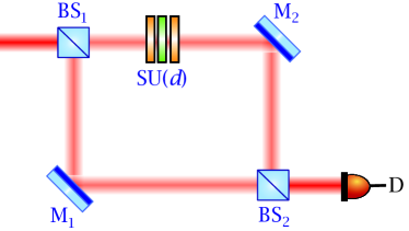
Figure 1: (Color online) Mach-Zehnder setup to interfere the state $\varrho$ (lower arm) with its SU($n$) transformed partners (upper arm). The distinguishability is related to the visibility of the interference pattern at the detector $D$.

Consequently, we define a Hilbert-Schmidt degree of polarization as

$$[\mathbb{P}_{\mathrm{HS}}^{(n)}]^{2}=\sup_{g\in\mathrm{SU(n)}}D^{2}_{\mathrm{HS}}(\rho,\rho_{g})=\mathop{\mathrm{Tr}}\nolimits(\rho^{2})-\inf_{g\in\mathrm{SU(n)}}\,\mathop{\mathrm{Tr}}\nolimits(\varrho\varrho_{g})\,.$$ (27)

The appealing point is that, formulated in this way, $\mathbb{P}_{\mathrm{HS}}^{(n)}$ depends on both the purity of the state and the distinguishability between the state and of its rotated counterparts. This later magnitude can be directly determined as the visibility of an interference experiment, as roughly schematized in Fig. 1. As unpolarized states are invariant under any SU($n$) transformation, this visibility (which is a measure of the distinguishability between $\varrho$ and $\varrho_{g}$) is zero for them.

III.1 Two-dimensional fields

Let us put the general definition to work for the 2D case. The state purity and the distinguishability can be expressed as

$$\mathop{\mathrm{Tr}}\nolimits(\varrho^{2})=\frac{1}{2}(1+|\mathbf{n}|^{2})\,,\quad\mathop{\mathrm{Tr}}\nolimits(\varrho\varrho_{g})=\frac{1}{2}(1+\mathbf{n}_{\varrho}\cdot\mathbf{n}_{\varrho_{g}})\,,$$ (28)

where $\mathbf{n}_{\varrho}$ and $\mathbf{n}_{\varrho_{g}}$ are the Stokes vectors associated with $\varrho$ and $\varrho_{g}$, respectively.

To find the minimum overlap, we follow a route that will be useful in extending this to the 3D case: one notices that any state $\varrho$ can be brought to a diagonal form $\varrho=R_{g_{0}}\varrho_{0}R^{\dagger}_{g_{0}}$, with $R_{g_{0}}$ being an SU(2) matrix and

$$\varrho_{0}=\frac{1}{2}\begin{pmatrix}1+|\mathbf{n}|&0\\ 0&1-|\mathbf{n}|\end{pmatrix}=\begin{pmatrix}\lambda_{+}&0\\ 0&\lambda_{-}\end{pmatrix}.$$ (29)

As $\inf_{g}\,\mathop{\mathrm{Tr}}\nolimits(\varrho\varrho_{g})=\inf_{g}\,\mathop{\mathrm{Tr}}\nolimits(\varrho_{0}\varrho_{0g})$, we get

$$\inf_{g\in\mathrm{SU(2)}}\mathop{\mathrm{Tr}}\nolimits(\varrho\varrho_{g})=\inf_{g\in\mathrm{SU(2)}}\frac{1}{2}(1+|\mathbf{n}|^{2}\cos\beta)=\frac{1}{2}(1-|\mathbf{n}|^{2})\,,$$ (30)

where $\beta$ is the corresponding Euler angle in (12). The minimum corresponds when $\mathbf{n}_{g}$ is the antipodal vector $\mathbf{n}_{g}=-\mathbf{n}$, as one might have anticipated. We thus conclude that

$$\mathbb{P}^{(2)}_{\mathrm{HS}}=|\mathbf{n}|=\lambda_{+}-\lambda_{-}\,,$$ (31)

which coincides with the standard definition (9).

Notice that in SU(2) we also have

$$\mathbb{P}^{(2)}_{\mathrm{HS}}=\textstyle{\frac{1}{2}}\displaystyle\inf_{g\in\mathrm{SU(2)}}\mathop{\mathrm{Tr}}\nolimits|\varrho-\varrho_{g}|\,,$$ (32)

which shows that the Hilbert-Schmidt $\mathbb{P}^{(2)}_{\mathrm{HS}}$ is proportional to the trace distance. This reinforces the connection to distinguishability as a measure of the degree of polarization, since the trace distance is a preferred metric to quantify the distinguishability between probability distributions Bengtsson and Życzkowski (2008).

III.2 Three-dimensional fields

Now, we have that

$$\mathop{\mathrm{Tr}}\nolimits(\varrho^{2})=\frac{1}{3}(1+2|\mathbf{n}|^{2})\,,\quad\mathop{\mathrm{Tr}}\nolimits(\varrho\varrho_{g})=\frac{1}{3}(1+2\mathbf{n}_{\varrho}\cdot\mathbf{n}_{\varrho_{g}})\,.$$ (33)

This last equation is surprisingly simple, but due to restrictions imposed by the su(3) algebra, $\mathbf{n}_{\varrho}$ and $\mathbf{n}_{\varrho_{g}}$ cannot be antiparallel. Thus, to optimize this distinguishability, we write again $\varrho=R_{g_{0}}\varrho_{0}R_{g_{0}}^{\dagger}$, with

$$\varrho_{0} = \frac{1}{3}\left(\begin{array}[]{ccc}1+\sqrt{3}n_{3}+n_{8}&0&0\\ 0&1-\sqrt{3}n_{3}+n_{8}&0\\ 0&0&1-2n_{8}\end{array}\right)$$ (37)

$$= \left(\begin{array}[]{ccc}\lambda_{1}&0&0\\ 0&\lambda_{2}&0\\ 0&0&\lambda_{3}\end{array}\right)\,,$$ (41)

with the eigenvalues sorted in decreasing order: $\lambda_{1}\geq\lambda_{2}\geq\lambda_{3}$. The vector $\mathbf{n}_{0}$ associated with $\varrho_{0}$ has two nonzero components: $n_{3}$ and $n_{8}$, and the minimum overlap depends now on these two parameters. In addition, positivity imposes

$$\max\left(-\frac{1+n_{8}}{\sqrt{3}},-\frac{2-n_{8}}{\sqrt{3}}\right) \leq n_{3}\leq \min\left(\frac{1+n_{8}}{\sqrt{3}},\frac{2-n_{8}}{\sqrt{3}}\right)\,,$$

$$-1 \leq n_{8}\leq \frac{1}{2}\,.$$ (42)

This defines a triangular region of the plane similar to the one investigated in Ref. Saastamoinen and Tervo (2004). The minimization is now more involved, and we distinguish two different situations:

III.2.1 $n_{3}=0$

This corresponds to a density matrix with two identical eigenvalues:

$$\varrho_{0}=\frac{1}{3}\left(\begin{array}[]{ccc}1+n_{8}&0&0\\ 0&1+n_{8}&0\\ 0&0&1-2n_{8}\end{array}\right)\,.$$ (43)

A direct numerical search shows that the minimum is reached when $\mathbf{n}_{g}$ is obtained from $\mathbf{n}_{0}$ by the linear transformation

$$\left(\begin{array}[]{c}n_{3g}\\ n_{8g}\\ \end{array}\right)=\frac{1}{2}\left(\begin{array}[]{cc}1&-\sqrt{3}\\ -\sqrt{3}&-1\\ \end{array}\right)\left(\begin{array}[]{c}n_{3}\\ n_{8}\\ \end{array}\right)\,,$$ (44)

so we have $\mathbf{n}\cdot\mathbf{n}_{g}=|\mathbf{n}|^{2}\cos(2\pi/3)=-n_{8}^{2}/2$. As explained above, the optimal angle between $\mathbf{n}_{0}$ and $\mathbf{n}_{0g}$ is not $\pi$ because this angle lies outside the permitted range. That not all angles are permitted can be explained by the fact that $\varrho_{0}$ and $\varrho_{0g}$ must have the same eigenvalues since they are unitarily related. One can confirm that the rotated vector $\mathbf{n}_{g}$ corresponds to the largest eigenvalue being permuted with one of the smaller. Hence, we can recast the infimum as Tr$(\varrho\varrho_{g})=2\lambda_{1}\lambda_{3}+\lambda_{3}^{2}$, so the degree becomes

$$\mathbb{P}^{(3)}_{\mathrm{HS}}=\lambda_{+}-\lambda_{-}\,,$$ (45)

where $\lambda_{+}=\lambda_{1}$ and $\lambda_{-}=\lambda_{3}$ (here, $\lambda_{2}=\lambda_{3}$). In this way, it appears as the natural generalization of the 2D version (9).

III.2.2 $n_{3}\neq 0$

The three eigenvalues are now different. We set $n_{8}=X\,n_{3}$ and write

$$\left(\begin{array}[]{cc}n_{3g}\\ n_{8g}\end{array}\right)=\left(\begin{array}[]{cc}\cos\theta&\sin\theta\\ \sin\theta&\cos\theta\end{array}\right)\left(\begin{array}[]{cc}-1&0\\ 0&1\end{array}\right)\left(\begin{array}[]{cc}n_{3}\\ n_{8}\end{array}\right)\,.$$ (46)

We have to consider three different zones:

• $X>1/\sqrt{3}$. The minimum is found when the angles $\beta_{1}$, $\beta_{2}$, and $\beta_{3}$ are respectively set to $(\pi,\pi,\pi)$ in the SU(3) matrix (II.2) and the rest of the angles equal 0. Then, $\theta=2\pi/3$ in (46) reproduces this minimum.

• $|X|<1/\sqrt{3}$. The minimum is now found when the angles $\beta_{1},\beta_{2}$ and $\beta_{3}$ take the values $(0,\pi,0)$ in (II.2). Here, $\theta=0$ in (46) gives the correct result.

• $X<-1/\sqrt{3}$. Here, the minimum occurs for $(\beta_{1},\beta_{2},\beta_{3})=(0,0,\pi)$, corresponding to the angle $\theta=-2\pi/3$ in (46).

The transformed density matrix accounts for a reshuffling of the eigenvalues and by simple inspection one can check that (45) holds for all three cases.

Additional insight can be gained by considering a three-dimensional plot illustrating the loci of the minima and a contour plot of these points, as shown in Fig. 2. The 6-fold symmetry of the result (corresponding to the six possible permutations of $\lambda_{1},\lambda_{2},\lambda_{3}$, so they remain in decreasing order) is explicit and quite similar to the symmetry exploited in Ref. Sheppard (2011).

The Hilbert-Schmidt degree (32) admits a direct 3D translation, namely,

$$\mathbb{P}^{(3)}_{\mathrm{HS}}=\textstyle{\frac{1}{2}}\displaystyle\inf_{g\in\mathrm{SU(3)}}\mathop{\mathrm{Tr}}\nolimits|\varrho-\varrho_{g}|\,.$$ (47)

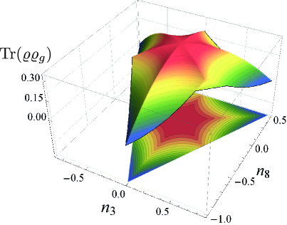
Figure 2: (Color online) A 3D plot locating the overlap $\mathop{\mathrm{Tr}}\nolimits(\varrho\varrho_{g})$ as a function of the parameters $n_{3}$ and $n_{8}$. At the bottom, we show a contour plot of the surface.

In this respect, it is worth stressing that several 3D measures have already been introduced in terms of the eigenvalues of the $3\times 3$ polarization matrix. Relevant examples are Sheppard (2011)

$$\mathbb{P}_{\mathrm{PP}}^{(3)}=\lambda_{1}-\lambda_{2}\,,\qquad\mathbb{P}_{\mathrm{U}}^{(3)}=3\lambda_{3}\qquad\mathbb{P}_{\mathrm{PU}}^{(3)}=2(\lambda_{2}-\lambda_{3})\,.$$ (48)

Here, $\mathbb{P}_{\mathrm{PP}}^{(3)}$ measures the strength of the pure polarized component, $\mathbb{P}_{\mathrm{U}}^{(3)}$ is the strength of the unpolarized component, and $\mathbb{P}_{\mathrm{PU}}^{(3)}$ is the strength of the component that is unpolarized within a plane. In Ref. Gamel and James , the method of majorization, previously used in quantum information, is applied to these measures to establish a partial ordering on the polarization state spaces.

Figure 3: (Color online) Isocontour lines (in the same color scale as in Fig. 2) of the different degrees of polarization as a function of the parameters $n_{3}$ and $n_{8}$. In the top panel, $\mathbb{P}_{\mathrm{HS}}^{(3)}$ (left) and $\mathbb{P}_{\mathrm{PP}}^{(3)}$ (right); in the bottom panel, $\mathbb{P}_{\mathrm{PU}}^{(3)}$ (left) and $\mathbb{P}_{\mathrm{U}}^{(3)}$ (right).

For the sake of completeness, in Fig. 3 we have plotted the lines of constant degrees of polarization for $\mathbb{P}_{\mathrm{HS}}^{(3)}$ and the three alternatives in (48), again as a function of $n_{3}$ and $n_{8}$. The figure is so explicit that it does not deserve many additional comments. What is really remarkable is how differently these measures quantify the polarization at the apices of the triangle.

IV Concluding remarks

We have explored the use of a degree of polarization based on the distance of a state to the set of its rotated counterparts. Such a definition is closely related to other recent proposals in different areas of quantum optics and is well behaved in the classical domain, providing an operational approach that can be extended from the 2D formalism (where it reproduces the standard results) to the 3D case (where it gives a new measure).

The resulting degree is tightly linked to the notion of distinguishability, which can be experimentally determined as the visibility in a simple interference setup, which confirms previous contentions along the same lines Klyshko (1992).

We hope that our analysis adds to and clarifies the discussion on measures of higher-dimensional polarization in the literature.

Appendix A Basic facts and parametrization of SU(3)

The su(3) algebra is usually presented in terms of a set of Hermitian generators known as the Gell-Mann matrices Weigert (1997) ${\Lambda}_{r}$ ($r=1,\ldots,8$). They obey the commutation relations

$$[{\Lambda}_{r},{\Lambda}_{s}]=2if_{rst}{\Lambda}_{t},$$ (49)

where, above and in the following, the summation over repeated indices applies. The structure constants $f_{rst}$ are elements of a completely antisymmetric tensor spelled out explicitly in Ref. Arvind et al. (1997), whose notation we follow.

A particular feature of the generators of SU(3) in the defining $3\times 3$ matrix representation is closure under anticommutation

$$\{{\Lambda}_{r},{\Lambda}_{s}\}=\frac{4}{3}\delta_{rs}{\openone}+2d_{rst}{\Lambda}_{t},$$ (50)

where $\delta_{rs}$ is the Kronecker symbol and $d_{rst}$ form a totally symmetric tensor Weigert (1997).

For the following, a vector-type notation is useful, based on the structure constants. The $f$ and $d$ symbols allow us to define both antisymmetric and symmetric products by

$$(\mathbf{A}\wedge\mathbf{B})_{r} = f_{rst}A_{s}B_{t}=-(\mathbf{B}\wedge\mathbf{A})_{r}\,,$$

$$(\mathbf{A}\star\mathbf{B})_{r} = \sqrt{3}d_{rst}A_{s}B_{t}=+(\mathbf{B}\star\mathbf{A})_{r}\,.$$

Given a density matrix ${\varrho}$ we can expand it in terms of the unit matrix $\openone$ and the ${\Lambda}_{r}$ in the form

$$\rho=\frac{1}{3}(1+\sqrt{3}\,\mathbf{n}\cdot{\bm{\Lambda}}).$$ (52)

This is the equivalent to the Bloch ball for SU(3). For a pure state the analogous Bloch sphere is defined by the condition

$$\mathbf{n}\cdot\mathbf{n}=1,\qquad\mathbf{n}\star\mathbf{n}=\mathbf{n}.$$ (53)

Thus, each pure qutrit state corresponds to a unique unit vector $\mathbf{n}\in\mathcal{S}^{7}$, the seven-dimensional unit sphere. In addition, this vector must obey the condition $\mathbf{n}\star\mathbf{n}=\mathbf{n}$, which places three additional constraints, thus reducing the number of real parameters required to specify a pure state from seven to four.

References

- Brosseau (1998) C. Brosseau, Fundamentals of Polarized Light: A Statistical Optics Approach (Wiley, New York, 1998).
- Mandel and Wolf (1995) L. Mandel and E. Wolf, Optical Coherence and Quantum Optics (Cambridge University Press, Cambridge, 1995).
- Ash and Nicholls (1972) E. A. Ash and G. Nicholls, Nature 237, 510 (1972).
- Pohl et al. (1984) D. W. Pohl, W. Denk, and M. Lanz, Appl. Phys. Lett 44, 651 (1984).
- Petruccelli et al. (2010) J. C. Petruccelli, N. J. Moore, and M. A. Alonso, Opt. Commun. 283, 4457 (2010).
- Samson (1973) J. C. Samson, Geophys. J. R. Astron. Soc. 34, 403 (1973).
- Barakat (1977) R. Barakat, Opt. Commun. 23, 147 (1977).
- Setälä et al. (2002a) T. Setälä, M. Kaivola, and A. T. Friberg, Phys. Rev. Lett. 88, 123902 (2002a).
- Setälä et al. (2002b) T. Setälä, A. Shevchenko, M. Kaivola, and A. T. Friberg, Phys. Rev. E 66, 016615 (2002b).
- Korotkova and Wolf (2004) O. Korotkova and E. Wolf, J. Opt. Soc. Am. A 21, 2382 (2004).
- Luis (2005) A. Luis, Opt. Commun. 253, 10 (2005).
- Ellis et al. (2005) J. Ellis, A. Dogariu, S. Ponomarenko, and E. Wolf, Opt. Commun. 248, 333 (2005).
- Réfrégier and Goudail (2006) P. Réfrégier and F. Goudail, J. Opt. Soc. Am. A 23, 671 (2006).
- Dennis (2007) M. R. Dennis, J. Opt. Soc. Am. A 24, 2065 (2007).
- Sheppard (2011) C. J. R. Sheppard, J. Opt. Soc. Am. A 28, 2655 (2011).
- Qian and Eberly (2011) X.-F. Qian and J. H. Eberly, Opt. Lett. 36, 4110 (2011).
- Gil (2007) J. J. Gil, Eur. Phys. J. Appl. Phys. 40, 1 (2007).
- Barakat (1983) R. Barakat, J. Mod. Opt. 30, 1171 (1983).
- Björk et al. (2002) G. Björk, J. Söderholm, A. Trifonov, P. Usachev, L. L. Sánchez-Soto, and A. B. Klimov, Proc. SPIE 4750, 1 (2002).
- Björk et al. (2000) G. Björk, S. Inoue, and J. Söderholm, Phys. Rev. A 62, 023817 (2000).
- Hillery (1987) M. Hillery, Phys. Rev. A 35, 725 (1987).
- Dodonov et al. (2000) V. V. Dodonov, O. V. Manko, V. I. Manko, and A. Wünsche, J. Mod. Opt. 47, 633 (2000).
- Marian et al. (2002) P. Marian, T. A. Marian, and H. Scutaru, Phys. Rev. Lett. 88, 153601 (2002).
- Vedral et al. (1997) V. Vedral, M. B. Plenio, M. A. Rippin, and P. L. Knight, Phys. Rev. Lett. 78, 2275 (1997).
- Marian and Marian (2008) P. Marian and T. A. Marian, Phys. Rev. A 77, 062319 (2008).
- Bellomo et al. (2012) B. Bellomo, G. L. Giorgi, F. Galve, R. Lo Franco, G. Compagno, and R. Zambrini, Phys. Rev. A 85, 032104 (2012).
- Gilchrist et al. (2005) A. Gilchrist, N. K. Langford, and M. A. Nielsen, Phys. Rev. A 71, 062310 (2005).
- Ma et al. (2009) Z. Ma, F.-L. Zhang, and J.-L. Chen, Phys. Lett. A 373, 3407 (2009).
- Monras and Illuminati (2010) A. Monras and F. Illuminati, Phys. Rev. A 81, 062326 (2010).
- Genoni et al. (2007) M. G. Genoni, M. G. A. Paris, and K. Banaszek, Phys. Rev. A 76, 042327 (2007).
- Mirbach and Korsch (1998) B. Mirbach and H. J. Korsch, Ann. Phys. 265, 80 (1998).
- Gnutzmann and Życzkowski (2001) S. Gnutzmann and K. Życzkowski, J. Phys. A 34, 10123 (2001).
- Wehrl (1978) A. Wehrl, Rev. Mod. Phys. 50, 221 (1978).
- Vedral (2002) V. Vedral, Rev. Mod. Phys. 74, 197 (2002).
- Ohya and Petz (2004) M. Ohya and D. Petz, Quantum Entropy and Its Use, 2nd ed. (Springer, Berlin, 2004).
- Bures (1969) D. Bures, Trans. Amer. Math. Soc. 135, 199 (1969).
- Uhlmann (1976) A. Uhlmann, Rep. Math. Phys. 9, 273 (1976).
- Wootters (1981) W. K. Wootters, Phys. Rev. D 23, 357 (1981).
- Braunstein and Caves (1994) S. L. Braunstein and C. M. Caves, Phys. Rev. Lett. 72, 3439 (1994).
- Życzkowski and Slomczyński (1998) K. Życzkowski and W. Slomczyński, J. Phys. A 31, 9095 (1998).
- Belavkin et al. (2005) V. P. Belavkin, G. M. D’Ariano, and M. Raginsky, J. Math. Phys. 46, 062106 (2005).
- Nielsen and Chuang (2010) M. A. Nielsen and I. L. Chuang, Quantum Computation and Quantum Information (Cambridge University Press, Cambridge, 2010).
- Witte and Trucks (1999) C. Witte and M. Trucks, Phys. Lett. A 257, 14 (1999).
- Ozawa (2000) M. Ozawa, Phys. Lett. A 268, 158 (2000).
- Bertlmann et al. (2002) R. A. Bertlmann, H. Narnhofer, and W. Thirring, Phys. Rev. A 66, 032319 (2002).
- Klimov et al. (2005) A. B. Klimov, L. L. Sánchez-Soto, E. C. Yustas, J. Söderholm, and G. Björk, Phys. Rev. A 72, 033813 (2005).
- Luis (2007) A. Luis, J. Opt. Soc. Am. A 24, 1063 (2007).
- Prakash and Chandra (1971) H. Prakash and N. Chandra, Phys. Rev. A 4, 796 (1971).
- Agarwal (1971) G. S. Agarwal, Lett. Nuovo Cimento 1, 53 (1971).
- Lehner et al. (1996) J. Lehner, U. Leonhardt, and H. Paul, Phys. Rev. A 53, 2727 (1996).
- Simon and Mukunda (1989) R. Simon and N. Mukunda, Phys. Lett. A 138, 474 (1989).
- Cornwell (1997) J. F. Cornwell, Group Theory in Physics, Vol. 1 (Academic Press, San Diego, 1997).
- Arvind et al. (1997) Arvind, K. S. Mallesh, and N. Mukunda, J. Phys. A 30, 2417 (1997).
- Rowe et al. (1999) D. J. Rowe, B. C. Sanders, and H. de Guise, J. Math. Phys 40, 3604 (1999).
- Dennis (2004) M. R. Dennis, J. Opt. A 6, S26 (2004).
- Li et al. (2012) X. Li, T.-H. Lan, C.-H. Tien, and M. Gu, Nat. Commun. 3, 998 (2012).
- Bengtsson and Życzkowski (2008) I. Bengtsson and K. Życzkowski, Geometry of Quantum States: An Introduction to Quantum Entanglement (Cambridge University Press, Cambridge, 2008).
- Saastamoinen and Tervo (2004) T. Saastamoinen and J. Tervo, J. Mod. Opt. 51, 2039 (2004).
- (59) O. Gamel and D. F. V. James, “Majorization and measures of classical polarization in three dimensions,” arXiv:1401.4733.
- Klyshko (1992) D. N. Klyshko, Phys. Lett. A 163, 349 (1992).
- Weigert (1997) S. Weigert, J. Phys. A 30, 8739 (1997).