Efficient boundary integral solution for acoustic wave scattering by irregular surfaces

Abstract

The left-right operator splitting method is studied for the efficient calculation of acoustic fields scattered by arbitrary rough surfaces. Here the governing boundary integral is written as a sum of left- and right-going components, and the solution expressed as an iterative series, expanding about the predominant direction of propagation. Calculation of each term is computationally inexpensive both in time and memory, and the field is often accurately captured using one or two terms. The convergence and accuracy are examined by comparison with exact solution for smaller problems, and a series of much larger problems are tackled. The method is also immediately applicable to other scatterers such as waveguides, of which examples are given.

Department of Applied Mathematics and Theoretical Physics, The University of Cambridge CB3 0WA, UK

1 Introduction

The calculation of acoustic scattering by extended rough surfaces remains a challenging problem both theoretically and computationally (e.g. [1, 2, 3, 4]) especially in the presence of strong multiple scattering. This becomes acute at low grazing angles, where multiple scattering occurs for very slight roughness. Boundary integral methods are flexible and often used for such problems but can be computationally intensive and scale badly with increasing wavenumber. Much effort has therefore been devoted to this aspect, where possible exploiting properties of the scattering regime. For forward scattering in 2-dimensions, for example, provided roughness length-scales are large, the ‘parabolic integral equation method’ can be applied [5, 6]. For electromagnetic problems, also formulated using boundary integrals, the methods of ordered multiple interactions and left-right splitting in both 2-d and 3-d ([7]-[13]) have been developed: here the scattered field is expressed as an iterative series of terms of increasing orders of multiple scattering, as described below. Approaches using conjugate gradient solutions combined with fast multilevel multipole are also receiving much attention. An important exception which overcomes the dependence of computational expense on wavenumber is [14], which has been applied to surfaces with piecewise constant impedance data or scattering in 2-d by convex polygons.

A versatile recursive technique known as Multiple Sweep Method of Moments was developed and analysed in [15, 16] where it was compared with Method of Ordered Multiple Interactions. This technique was shown to tackle ‘composite’ problems for which the above method diverges such as for a ship on a rough sea surface. Other iterative solutions have been studied in [17]. In addition theoretical results are available in various limiting regimes (e.g. perturbation theory for small surface heights, $k\sigma\ll 1$ including periodic surfaces [18, 19, 20], Kirchhoff approximation [21, 22], or the small slope approximation [23] which is accurate over a wider range of scattering angles than both of these). For arbitrary finite rough surfaces, however, validation is more difficult, and such results are therefore scarce.

In this paper the Left-Right Splitting method is developed and applied to the problem of acoustic scattering in three dimensions by randomly rough surfaces. For relatively small surfaces the results are validated by comparison with numerical solution of the full boundary integral equation. The principal aims are to validate the approach; to examine its robustness and convergence as the angle of incidence changes; and to consider further approximations which may reduce the computation time. The approach is applicable to a wide range of interior and exterior scattering problems, and we give examples for acoustic propagation in a varying duct, in addition to scattering from large rough surfaces.

The mathematical principles of the method are the same as for the two-dimensional problem [9] although implementation is considerably more complicated: The unknown field $\psi$ on the surface is expressed as the solution to the Helmholtz integral equation, with the integration taken over the rough surface. This may be written formally as $A{\psi}={{\psi_{inc}}}$, where ${{\psi_{inc}}}$ is the incident field impinging (say) from the left, so that we require ${\psi}=A^{-1}{{\psi_{inc}}}$. The region of integration is split into two, to the left and right of the point of observation, allowing $A$ to be written as the sum of ‘left’ and ‘right’ components, say $(L+R){\psi}={\psi_{inc}}$. Roughly speaking $L$ represents surface interactions due to scattering from the left, and $R$ the residual scattering from the right. The inverse of $A$ can formally be expressed as a series

$$A^{-1}=L^{-1}-L^{-1}RL^{-1}+...$$ (1)

Discretization of the integral equation yields a block matrix equation, in which $L$ is the lower triangular part of the block matrix $A$ (including the diagonal) and $R$ is the upper triangular part. Under the assumption that most energy is right-going, $L$ is the dominant part of $A$, and the series can be truncated to provide an approximation for ${\psi}$. This approach has several advantages. In terms of wavelength $\lambda$, evaluation of each term scales with the fourth rather than the sixth power of $\lambda$ required for $A^{-1}$; subsequent terms (of which typically only the first one or two are needed) have the same computational cost. With further approximations this can be reduced to $\lambda^{3}$. However, this operation count is only part of the story, because the low complexity and memory requirement allow very large problems to be tackled without such additional approximation. In addition the algorithm lends itself well to parallelisation, and the speed scales approximately linearly with the number of processors.

In §2 the governing equations and left-right splitting approximation are formulated. The numerical details and main results are shown in §3.

2 Formulation of equations

Consider a 3-dimensional medium with horizontal axes $x,y$ and vertical axis $z$ directed upwards, and let $k$ be the wavenumber. Let $S=s(x,y)$ be a 2-dimensional rough surface, varying about the plane $z=0$, which is continuous and differentiable as a function of $x,y$ (see Figure 1). (Arbitrary scatterers can also be treated by the methods shown here; examples will be given later.) Consider a time-harmonic acoustic wave $\psi$, obeying the wave equation $(\nabla^{2}+k^{2})\psi=0$ in the region $z>s(x,y)$, resulting from an incident wave ${\psi_{inc}}$ at a small grazing angle $\theta$ to the horizontal plane. This may for example be a plane wave or a finite beam. The axes can be chosen so that the principal direction of propagation is at a small angle to the $(x,z)$ plane.

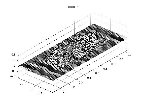
Figure 1: Example rough surface

We will treat the Neumann boundary condition, i.e. an acoustically hard surface. The derivation for the Dirichlet condition is similar. Thus

$${\partial\psi\over\partial{\bf n}}=0$$ (2)

where ${\bf n}$ is the outward normal (i.e. directed out of the region $z>s(x,y)$). The free space Green’s function is given by

$$G({\bf r},{\bf r}^{\prime})={e^{ik|{\bf r}-{\bf r}^{\prime}|}\over 4\pi|{\bf r}-{\bf r}^{\prime}|}.$$ (3)

The field at a point ${\bf r}$ in the medium is related to the surface field by the boundary integral

$$\psi_{inc}({\bf r})=\psi({\bf r})-\int_{S}{\partial G({\bf r},{\bf r}^{\prime})\over\partial n}\psi({\bf r}^{\prime})d{\bf r}^{\prime}$$ (4)

where ${\bf r}=(x,y,z)$ and ${\bf r}^{\prime}=(x^{\prime},y^{\prime},s(x^{\prime},y^{\prime}))$, say, and taking the limit as ${\bf r}\rightarrow{\bf r}_{s}$ gives

$$\psi_{inc}({\bf r}_{s})=\psi({\bf r}_{s})-\int_{S}{\partial G({\bf r}_{s},{\bf r}^{\prime})\over\partial n}\psi({\bf r}^{\prime})d{\bf r}^{\prime}$$ (5)

where now ${\bf r}_{s}=(x,y,s(x,y))$. The integrand is singular at the point ${\bf r}^{\prime}={\bf r}_{s}$, and we must take care to interpret this integral as the limit of the integral in eq. (4) as ${\bf r}\rightarrow{\bf r}_{s}$.

In order to treat the equation numerically it is convenient to write the integration with respect to $x$,$y$, so that eq. (5) becomes

$$\psi_{inc}({\bf r}_{s})=\psi({\bf r}_{s})-\int_{-\infty}^{\infty}\int_{-\infty}^{\infty}{\partial G({\bf r}_{s},{\bf r}^{\prime})\over\partial n}\psi({\bf r}^{\prime})~{}\gamma({\bf r}^{\prime})dx^{\prime}dy^{\prime}$$ (6)

where (with very slight abuse of notation)

$$\gamma({\bf r}^{\prime})=\sqrt{1+\left({\partial s\over\partial x^{\prime}}\right)^{2}+\left({\partial s\over\partial y^{\prime}}\right)^{2}}.$$ (7)

and the expression under the square root is evaluated at ${\bf r}^{\prime}$.

2.1 Formal solution and splitting series

The method of solution is analogous to that applied to the electromagnetic problem in 2-d or 3-d [9, 12]. The governing integral equation (6) is expressed in terms of right- and left-going operators $L$ and $R$ with respect to the $x$-direction:

$$\psi_{inc}({\bf r}_{s})=A\psi\equiv(L+R)\psi$$ (8)

where $L$ and $R$ are defined (for an $L^{2}$ function $f$) by

$$Lf({\bf r}) = f-\int_{-\infty}^{\infty}\int_{-\infty}^{x}{\partial G({\bf r},{\bf r}^{\prime})\over\partial n}f({\bf r}^{\prime})~{}\gamma({\bf r}^{\prime})~{}dx^{\prime}~{}dy^{\prime},$$ (9)

$$~{}~{}~{}~{}~{}Rf({\bf r}) = -\int_{-\infty}^{\infty}\int_{x}^{\infty}{\partial G({\bf r},{\bf r}^{\prime})\over\partial n}f({\bf r}^{\prime})~{}\gamma({\bf r}^{\prime})~{}dx^{\prime}~{}dy^{\prime}$$ (10)

and ${\bf r}=(x,y,z)$, ${\bf r}^{\prime}=(x^{\prime},y^{\prime},s(x^{\prime},y^{\prime}))$. [For notational conveneince $L$ is interpreted to include the contribution from the singularity arising in (5) when ${\bf r}\rightarrow{\bf r}^{\prime}$.]

The region of integration is thus split into two with respect to $x$, and the solution of equation (8) can be expanded as a series, given by

$$\psi=(L+R)^{-1}\psi_{inc}=\left[L^{-1}-L^{-1}RL^{-1}+...\right]\psi_{inc}.$$ (11)

The key observation is that at fairly low grazing angles the effect of ${\bf R}$ is in some sense small, so that the series converges quickly and can be truncated. Define the $n$-th order approximation as

$$\psi_{n}=\sum_{1}^{n}~{}L^{-1}\left(RL^{-1}\right)^{n-1}~{}{\psi_{inc}}.$$ (12)

[Note that $L$ and $R$ depend on surface geometry and wavenumber only, not on incident field; and that one might expect convergence of the series (11) for given ${\psi_{inc}}$ but not uniform (norm) convergence of the series (1).] This corresponds physically to an assumption that surface-surface interactions are dominated by those ‘from the left’, as expected in this scattering regime. $L$ is large compared with $R$ first, because $L$ includes the dominant ‘diagonal’ value; second because a predominantly right-going wave gives rise to more rapid phase-variation in the integrand in $R$ than in $L$. (Although this depends on surface geometry and cannot in general be quantified precisely, it occurs because in (5) the phase in the Green’s function kernel decreases as the observation point is approached from the left and then increases to the right; whereas the phase of $\psi$ tends to increase throughout, like that of the incident field.) This is borne out numerically, with many cases of interest well-described using only one or two terms of the series.

The scattered field due to a given approximation $\psi_{n}$ is obtained by substitution back into the boundary integral (4). It is helpful to consider the significance of successive approximations to this field in the ray-theoretic limit: The first iteration contains ray paths which, before leaving the surface, may have interacted with the surface arbitrarily many times but only in a forward direction. The second includes most paths which have changed direction twice: once via the operator $R$ and again via $L^{-1}$; and so on (see Figure 2). Thus the first iteration accounts for multiple scattering but not reversible paths which can occur when incident and backscatter direction are opposite; these paths occur in pairs of equal length and therefore add coherently, giving rise to a peak in the backscattered direction (enhanced backscatter eg [24, 25]) in strongly scattering regimes. We would therefore expect this to show initially at the second approximation.

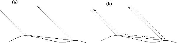
Figure 2: Possible paths (a) at 1st iteration, and (b) at 2nd iteration when reversible paths can occur and add coherently.

Having obtained this series, numerical treatment by surface discretization is straightforward. (Discretization can equivalently be carried out before the series expansion, but it is more convenient, and analytically more transparent, to expand the integral operator first.)

3 Numerical solution and results

Although use of the series (11) is motivated by physical considerations and its terms provide a convenient theoretical interpretation, the immediate advantage is computational: if the surface is discretized using a rectangular grid of $M$ by $N$ points, with $M$ transverse steps ($y$ direction) and $N$ in range ($x$), then $(L+R)$ becomes an $(MN\times MN)$ matrix, and exact inversion would take $O((MN)^{3})$ operations. On the other hand evaluation of each term of eq. (11) involves inversion of an $M\times M$ matrix at each of $N$ range steps, requiring just $O(NM^{3})$ operations and far less memory. Assuming a resolution of say 10 points per wavelength, this scales with $\lambda^{4}$. There is an additional ‘matrix filling’ component; this also increases with $\lambda^{4}$, and in practice this is the dominant computational cost in the left-right splitting algorithm (typically more than 90% when $M\cong N$).

3.1 Numerical solution

The numerical treatment will now be outlined. The notation $L$, $R$ will be used to refer to the discretized forms of the integral operators where no confusion arises, and we will focus on solution of the first term of (11), i.e. inversion of $L$. Although not evaluated explicitly as such, the matrix $L$ is conveniently viewed as an $N\times N$ lower-triangular block matrix whose entries are $M\times M$ matrices. The system can therefore be inverted by Gaussian elimination and back-substitution. This is an $N$-step ‘marching’ process, in which each diagonal $M\times M$ block is inverted in turn, corresponding to marching the solution for the unknown surface field in the positive $x$ direction. Choosing step-sizes $\Delta x$, $\Delta y$ we define

$$x = x_{1},...,x_{N},~{}~{}~{}~{}~{}~{}x_{n}=n\Delta x$$ (13)

$$y = y_{1},...,y_{M},~{}~{}~{}~{}~{}~{}y_{m}=m\Delta y.$$ (14)

Denote the discretized surface values by

$${\psi_{inc}}(x_{n},y_{m}) =a_{nm}$$ (15)

$$\psi(x_{n},y_{m}) =b_{nm},$$ (16)

denote the area of each subintegration region by $\delta=\Delta x\Delta y$, and write $\sigma_{ij}=~{}\gamma({\bf r}_{ij})$ where $\gamma$ (equation (7)) is evaluated at the point ${\bf r}_{ij}=(x_{i},y_{j},s(x_{i},y_{j}))$. This induces a discretization of (8) and at each point surface point $s(x_{n},y_{m})$ we get

$$a_{nm}=\sum_{i=1}^{N}\sum_{j=1}^{M}~{}A_{nmij}~{}b_{ij}$$ (17)

where

$$A_{nmij} = \Delta x\Delta y~{}\sigma_{ij}\partial G({\bf r}_{nm},{\bf r}_{ij})/\partial n~{}~{}~{}~{}~{}~{}~{}~{}~{}~{}~{}~{}~{}~{}(n\neq i,~{}{\rm or}~{}m\neq i)$$ (18)

$$A_{nmnm} = -\left[{1\over 2}-{\delta\over\sigma_{ij}^{2}}(s_{xx}+s_{yy})\right]$$ (19)

and again ${\bf r}_{ij}=(x_{i},y_{j},s(x_{i},y_{j}))$. For each value of $n$ this gives a set of $M$ equations. Retaining just the first term in the iterative series (11),

$$\psi\cong L^{-1}{\psi_{inc}},$$ (20)

yields a set of equations identical to (17) except that the sum over $i$ has upper limit $n$:

$$a_{nm}=\sum_{i=1}^{n}\sum_{j=1}^{M}~{}A_{nmij}~{}b_{ij}.$$ (21)

This is equivalent to integration over the half plane to the left of the line of observation ($x^{\prime}\leq x_{n})$. Now at each range step $x_{n}$, assuming that we have obtained the values $b_{im}$ for $i<n$, equation (21) can be rearranged to give

$$a_{nm}-\sum_{i=1}^{n-1}\sum_{j=1}^{M}~{}A_{nmij}~{}b_{ij}=\sum_{j=1}^{M}~{}A_{nmnj}~{}b_{nj}$$ (22)

for $m=1,...,M$. Everything on the left-hand-side is known or has been found at previous steps. For each $n$ this gives a matrix equation, which we rewrite for convenience as

$${\bf c}_{n}=B_{n}{\bf b}_{n}$$ (23)

where the subscript $n$ indicates dependence on $x_{n}$ and we have written the vectors in bold. Therefore, ${\bf b}_{n}$ denotes solution values $\psi(x_{n},y)$ at the range step $x_{n}$, and $B_{n}$ is the $M\times M$ matrix (the $n$-th term on the diagonal of $L$) with elements

$$\left(B_{n}\right)_{mj}=A_{nmnj}.$$ (24)

We thus require

$${\bf b}_{n}=B_{n}^{-1}{\bf c}_{n}$$ (25)

for each $n$. We solve (25) in turn for $n=1,...,N$, using each result to redefine the left-hand-side of eq. (23) and thus find the surface field as defined by (20). Subsequent terms in the series (11) are evaluated in exactly the same way, with the ‘driving’ term ${\psi_{inc}}$ replaced by $R$ times the result of the previous evaluation.

3.2 Computational results

One of the main applications is to irregular or randomly rough surfaces (for example sea surfaces or terrain). Statistically stationary surfaces with Gaussian statistics (normally distributed heights) are easily generated computationally with any prescribed spatial autocorrelation function (a.c.f.) $\rho(\xi,\eta)$, where

$$\rho(\xi,\eta)=<s(x,y)~{}s(x+\xi,y+\eta)>.$$ (26)

Here the angled brackets denote ensemble averages. For simplicity we have used an isotropic two-dimensional Gaussian a.c.f., $\rho(\xi,\eta)=\exp(-[\xi^{2}+\eta^{2}]/l^{2})$ where $l$ defines a correlation length. In order to minimise and distinguish edge effects we used surfaces which become flat at the outer edge; this is not necessary for the method to be applicable. Studies included the strongly scattering regime of surfaces with both correlation length and r.m.s. height of the order of a wavelength. With the exception of parallel code mentioned later, all tests were run on a desktop Pentium 4 3.2GHz machine with 1GB memory running Linux.

Comparison was made first against the full or ‘exact’ inversion of the boundary integral. The quantity used for the comparison was the surface field. Because of the high computational cost of full inversion this comparison was carried out for a relatively small surface of $12\times 12$ wavelengths, using a grid of $120\times 120$ points. Here the r.m.s. height and correlation length are approximately equal to $\lambda$. Contour plots of the amplitude of $\psi$ calculated by the two methods is shown in Figure 3. One iteration of the left-right series took around 7 seconds, whereas “exact” full inversion took around 23 minutes. (The full inversion code at double precision ran out of memory at this stage so, in this case only, the matrix was evaluated in single precision. Iterative code remains in double precision throughout.)

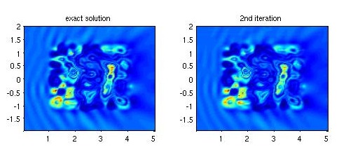
Figure 3: Shaded contour plot of the amplitude of the surface fields by (a) exact and (b) iterative solution (2 terms), for surface with r.m.s. height and correlation length approximately equal to $\lambda$.

In order to illustrate the convergence, comparison of field values along the mid-line in the $x$-direction is shown in Figure 4 for the first 4 iterations. In this case the incident field was a plane wave impinging at an angle of 10^o from grazing. Extremely good agreement is found. Notice that the oscillatory behaviour at the left is captured at the 2nd but not the 1st iteration. (It should be emphasized that although we found no divergent cases, convergence is not necessarily guaranteed. For electromagnetic waves the method [10] exhibited divergences apparently due to resonant surface features.)

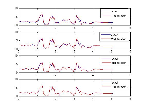
Figure 4: Comparison between exact and successive terms of the left-right solution corresponding to Fig. 3, along a line in $x$-direction, for grazing angle $10^{o}$.

The solution for an field incident at $45^{o}$ impinging on the same surface is shown in Figure 5, and again converges rapidly.

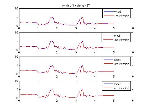
Figure 5: Comparison for surface as in Figure 4, for grazing angle of $45^{o}$.

A further comparison (Figure 6) using a ‘smoother’ surface, with the same correlation lengths but r.m.s. height reduced to $\lambda/20$, at $10^{o}$ from grazing, gives similarly close agreement.

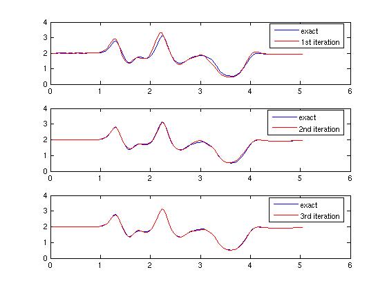
Figure 6: Comparison between exact and successive terms of the left-right solution, for grazing angle $10^{o}$ due to a smoother surface with r.m.s. height $\lambda/20$.

We now consider the application of the code to larger surfaces, in order further to examine timings and rates of convergence as functions of incident angle. Evaluations of the first iterates were carried out for several cases. As mentioned above, the two main components of the calculation are a $N$ matrix inversion and a set of Green’s functions evaluation, at each of $N$ range steps. The matrix inversion remained a small percentage of the cost in all cases, and computation time should increase with the square of the number of unknowns, $M^{2}N^{2}$. The actual computation times were found to conform closely to this, as shown in Table 1. Times in the second column, corresponding to the simple optimised integration as described below, should be regarded as applicable for most surface geometries, and can easily be reduced further with higher order schemes.

No. of unknowns	Solution time	Optimised integration
120x120	6.9	2.6
240x160	48	17
240x320	198	70
480x320	774	265
480x480	1752=29.2min	605=10.1min
1000x1000	31870=8.5hrs	10992 = 3hrs

Table 1: Computation time on desktop computer

Note that the algorithm is easily parallelised: the integration, to which the bulk of computation time is devoted, can be shared among any number of processors. This has been carried out using MPI on a Sunfire machine, and as expected the computation speed increases linearly with the number of processors. Solution for around $5\times 10^{6}$ unknowns, on a waveguide of 550 $\lambda$ in length and 80 $\lambda$ circumference, was obtained in 5.3 hours with standard integration and under 2 hours using the optimised integration below, on 96 processors.

Strategies are available for reduction of the Green’s function evaluation cost. One of these is fast multilevel multipole, which can reduce the time-dependence to $O(NM\log NM)$, but we found this to have certain disadvantages including relatively high complexity and memory cost, and accuracy which is not easily regulated. A much simpler expedient which retains the order of dependence on the number of unknowns, but reduces the multiplier, is the following: A simple quadrature using all available points was initially used to carry out the integration for the left-hand-side of eq. (25). The integrand, however, is relatively smooth as a function of transverse coordinate, and this increases with spatial separation in $x$. Thus as the marching solution proceeds, we can use higher-order integration schemes utilising far fewer points with little loss of accuracy. Even a simple trapezium rule, for example, operating on half the number of points reduced the computation time by a factor of 3 and resulted in errors of well under 1%. We calculated surface fields on a desktop computer for a surface of $48\lambda\times 48\lambda$ (230,000 unknowns) in around 10 minutes, and $100\lambda\times 100\lambda$ ($10^{6}$ unknowns) in 180 minutes.

The same method is applicable to exterior and interior scattering problems due to various large scatterers and geometries. Most such geometries involve even better-behaved integrals, and are therefore amenable to the above integration strategy. Solution for the much larger problem of a waveguide of around 150 wavelengths in length and diameter 20 wavelengths (not shown) was calculated on the desktop computer in around 140 minutes.

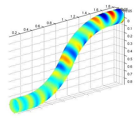
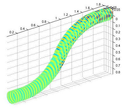
Figure 7: Real part of surface field on waveguide at two frequencies.

4 Conclusions

The paper describes the development and application of the left-right splitting algorithm for acoustic scattering by rough perfectly reflecting surfaces and other complex scatterers. Results have been validated by comparison with “exact” numerical solutions, and by examining the convergence of the series. The formulation is physically-motivated to apply to incident fields at low grazing angles, although good convergence has been obtained at angles close to normal incidence. Problems involving up to $10^{6}$ unknowns or more can be solved relatively simply on a standard desktop computer, and much larger problems still in a few hours on a parallel machine.

The cost of the method scales with the square of the number of unknowns; this can be improved by application of, say, fast multipole methods, but this has not been necessary as in this approach the multiplier is relatively small and can be further reduced by optimising the integrations.

The terms in the series represent increasing orders of surface interaction, and this is likely to provide further insight into multiple scattering mechanisms.

Acknowledgements

The authors acknowledge partial funding from the DTI eScience programme, and use of the Cambridge-Cranfield High Performance Computer Facility. Many of the ideas arose out of a previous electromagnetic project supported by BAE Systems and MS is grateful for many helpful discussions.

Figure Captions

Figure 1: Example rough surface.

Figure 2: Possible paths (a) at 1st iteration, and (b) at 2nd iteration when reversible paths can occur and add coherently.

Figure 3: Shaded contour plot of the amplitude of the surface fields by (a) exact and (b) iterative solution (2 terms), for surface with r.m.s. height and correlation length approximately equal to $\lambda$.

Figure 4: Comparison between exact and successive terms of the left-right solution corresponding to Fig. 3, along a line in $x$-direction, for grazing angle $10^{o}$.

Figure 5: Comparison for surface as in Figure 4, for grazing angle of $45^{o}$.

Figure 6: Comparison between exact and successive terms of the left-right solution, for grazing angle $10^{o}$ due to a smoother surface with r.m.s. height $\lambda/20$.

Figure 7: Real part of surface field on waveguide at two frequencies.

References

- [1] J. A. Ogilvy, The Theory of Wave Scattering from Random Rough Surfaces (IOP Publishing, Bristol, 1991).
- [2] A.G. Voronovitch, Wave Scattering from Rough Surfaces (Springer, Berlin, 1994).
- [3] K.F. Warnick & W.C. Chew, Numerical methods for rough surface scattering, Waves in Random Media, 11, R1-R30 (2001).
- [4] M. Saillard & A. Sentenac, Rigorous solutions for electromagnetic scattering from rough surfaces, Waves in Random Media, 11, R103-R137 (2001).
- [5] E. Thorsos, Rough surface scattering using the parabolic wave equation, J. Acoust. Soc. Am., Suppl. 1 82, S103 (1987).
- [6] M. Spivack, Moments and angular spectrum for rough surface scattering at grazing incidence, J. Acoust. Soc. Am., 97, 745-753 (1995).
- [7] D.A. Kapp & G.S. Brown, A new numerical method for rough surface scattering calculations, IEEE Trans. Ant. Prop., 44, 711-721 (1996).
- [8] M. Spivack, Forward and inverse scattering from rough surfaces at low grazing incidence J. Acoust. Soc. Am., 95 Pt 2, 3019 (1994).
- [9] M. Spivack, A. Keen, J. Ogilvy, & C. Sillence, Validation of left-right method for scattering by a rough surface, J Modern Optics 48 1021-1033 (2001).
- [10] P. Tran, Calculation of the scattering of electromagnetic waves from a two-dimensional perfectly conducting surface using the method of ordered multiple interaction, Waves in Random Media, 7, 295-302 (1997).
- [11] R.J Adams & G.S. Brown, A combined field approach to scattering from infinite elliptical cylinders using the method of ordered multiple interactions IEEE Trans. Ant. Prop., 47, 364-375 (1999).
- [12] M. Spivack, J. Ogilvy, & C. Sillence, C., Electromagnetic scattering by large complex scatterers in 3D, IEE Proc Science, Measurement & Tech 151 464-466 (2004).
- [13] M.R. Pino, L. Landesa, J.L. Rodriguez, F. Obelleiro, & R.J. Burkholder, The generalized forward-backward method for analyzing the scattering from targets on ocean-like rough surfaces IEEE Trans. Ant. Prop., 47, 961-969 (1999).
- [14] S N Chandler-Wilde, S Langdon, & L Ritter, A high-wavenumber boundary-element method for an acoustic scattering problem, Phil Trans R Soc Lond A 647-671 (2004).
- [15] D. Colak, R.J. Burkholder, & E.H. Newman, On the convergence properties of multiple sweep method of moments scattering from 3D targets on ocean-like rough surfaces, Appl. Comp. Electromag. Soc. J. 22, 207-218 (2007).
- [16] D. Colak, R.J. Burkholder, & E.H. Newman, Multiple sweep method of moments analysis of electromagnetic scattering from 3D targets on ocean-like rough surfaces, Microwave and Opt Tech Lett 49, 241-247 (2007).
- [17] C. Macaskill & B.J. Kachoyan, Iterative approach for the numerical simulation of scattering from one- and two-dimensional rough surfaces, Appl. Opt., 32, 2839-2847 (1993).
- [18] E.I. Thorsos & D.R. Jackson, The validity of the perturbation approximation for rough surface scattering using a Gaussian roughness spectrum, J. Acoust. Soc. Am., 86, 261-277 (1989).
- [19] R.L. Holford, Scattering of sound waves by a periodic, pressure release surface: an exact solution, J. Acoust. Soc. Am., 70, 1116-1128 (1981).
- [20] J.A. DeSanto, Scattering from a perfectly reflecting arbitrary periodic surface - an exact theory, Radio Science, 16, 1315-1326 (1981).
- [21] W.C. Meecham, On the use of the Kirchhoff approximation for the solution of reflection problems J. Rat. Mech. Anal, 5, 323-334 (1956).
- [22] E.I. Thorsos, The validity of the Kirchhoff approximation for rough surface scattering using a Gaussian roughness spectrum, J. Acoust. Soc. Am., 83, 78-92 (1988).
- [23] A.G. Voronovich, Non-local small-slope approximation for wave scattering from rough surfaces, Waves in Random Media, 6, 151-167 (1996).
- [24] A.A. Maradudin, T. Michel, A.R. McGurn & E.R. Mendez, Enhanced backscattering of light from a random grating, Ann Phys, 203, 255-307 (1990).
- [25] C. Macaskill, Geometrical optics and enhanced backscatter from very rough surfaces, J Opt Soc Am A, 8, 88-96 (1991).