Washing out of the $0$-$\pi$ transition in Josephson junctions

Abstract

We consider a Josephson junction formed by a quantum dot connected to two bulk superconductors in presence of Coulomb interaction and coupling to both an electromagnetic environment and a finite density of electronic quasi-particles. In the limit of large superconducting gap we obtain a Born-Markov description of the system dynamics. We calculate the current-phase relation and we find that the experimentally unavoidable presence of quasi-particles can dramatically modify the $0$-$\pi$ standard transition picture. We show that photon-assisted quasi-particles absorption allows the dynamic switching from the $0$- to the $\pi$-state and vice-versa, washing out the $0$-$\pi$ transition predicted by purely thermodynamic arguments.

Introduction.— The Josephson junction is a fundamental element of superconducting quantum nano-electronics, with a wide spectrum of applications ranging from quantum information to medical imagery. Such a junction can be formed by contacting two superconductors by a large variety of nano-structures Kasumov et al. (1999); Steinbach et al. (2001); Goffman et al. (2000); van Dam et al. (2006); Pillet et al. (2010); Deacon et al. (2010); Basset et al. (2014). A fruitful way to describe transport through the device is to consider the formation of electronic bound states at the junction known as Andreev bound states. In thermodynamic equilibrium, at low temperatures, and for short junctions the current-phase relation is determined mainly by the phase dependence of the lowest energy Andreev bound state. A wealth of experimental and theoretical work has been devoted to investigate the current-phase dependence in Josephson junctions and leads, for instance, to the prediction Bulaevskii et al. (1977); Rozhkov et al. (2001); Buzdin (2005); Martín-Rodero and Levy Yeyati (2011) and the observation Baselmans et al. (1999); Ryazanov et al. (2001); Kontos et al. (2002); van Dam et al. (2006); Cleuziou et al. (2006); Jorgensen et al. (2007) of a change of sign of the current-phase relation, the so called 0-$\pi$ transition. This can be induced by the presence of magnetic moments (magnetic impurities or ferromagnetic layer) or in a non-magnetic material by the repulsive Coulomb interaction at the quantum dot forming the junction, as is observed in carbon nanotubes Cleuziou et al. (2006); Eichler et al. (2009); Maurand et al. (2012); Pillet et al. (2013) or semiconducting nanowire van Dam et al. (2006) Josephson junctions. At the basis of this transition is the change of the parity of the junction. In superconductors electrons are paired, but if in the quantum dot forming the Josephson junction, Coulomb repulsion is sufficiently large, the ground state will accommodate only one electron. At lowest order in the tunnelling, the Josephson current is suppressed, and at the next (4th) order it changes sign Rozhkov et al. (2001), since Cooper pairs are re-composed by tunnelling with reversed spins.

Only recently a direct detection of the excited Andreev bound states has been possible with a series of experiments that probed the Josephson junction by resonating microwaves irradiation Bretheau et al. (2013a, b). These experiments pointed out the importance of the coupling to the electromagnetic (EM) environment and in particular to the quasi-particles present in the superconducting leads. It is an established experimental fact that the density of quasi-particles does not vanish exponentially with the temperature as predicted by the BCS theory, but remains finite, even at the lowest temperatures Ristè et al. (2013); Olivares et al. (2014). Environment-assisted absorption of quasi-particles can modify the junction parity, since an unpaired electron can fall in the quantum-dot. This process has been considered very recently for junctions where Coulomb interaction is negligible Olivares et al. (2014).

In this paper, we investigate the effect of parity transitions induced by the quasi-particle absorption and emission in presence of Coulomb interaction. We consider the limit for which the superconducting gap is the largest energy scale, also known as atomic limit. We obtain an exact Born-Markov description of the system coupled to the EM environment. In this approximation, the $\pi$-phase is indicated by the occupation of an odd-parity state with a vanishing of the supercurrent. This allows to describe in a consistent way the $0$-$\pi$ transition by taking into account the relaxation processes that induce parity changes. We find that the presence of quasi-particles can completely wash out the $0$-$\pi$ transition, and invalidate the usual arguments based on the parity of the lowest energy state. The quasi-particles are necessary to let the system relax to the lowest energy ground state, but at the same time, they allow dynamic transitions between states, smoothening the transition. We also considered the effect of the irradiation of a microwave signal on the gate of the quantum dot that can be used to probe the state of the junction in both the $0$- and $\pi$- phase.

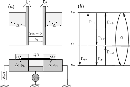
Figure 1: (a) Representation of the Josephson junction formed, for instance, by a carbon nanotube quantum dot bridging two superconductors. (b) Schematics of the transitions between the Andreev bound states induced by incoherent $\Gamma_{ij}$ and coherent $\Omega$ perturbations.

Model.— Let us consider a quantum dot with a single electronic level forming a Josephson junction between two superconducting leads [see Fig. 1-(a)]. We assume that the junction is phase biased, that a time-dependent gate voltage can be applied, and that the source-drain circuit is shunted on an impedance $Z(\omega)$. This system can be modeled by the (time dependent) Hamiltonian

$$H=H_{\rm dot}(t)+H_{\rm L}+H_{\rm R}+H_{\rm T}+H_{\rm B}+H_{\rm c}\,.$$ (1)

The first term of Eq. (1) reads $H_{\rm dot}(t)=\epsilon_{d}(t)(n_{\uparrow}+n_{\downarrow})+Un_{\uparrow}n_{\downarrow}$ and it describes the single-electronic level of time-dependent energy $\epsilon_{d}(t)=\epsilon_{0}+\epsilon_{1}\cos(\omega t)$ and Coulomb repulsion $U$. Here $n_{\sigma}=d_{\sigma}^{\dagger}d_{\sigma}$, and $d_{\sigma}$ is the electronic destruction operator on the dot of spin projection $\sigma$. The second and third terms $H_{X}=\sum_{k\sigma}\xi_{Xk}c_{Xk\sigma}^{\dagger}c^{\phantom{{\dagger}}}_{Xk\sigma}+\sum_{k}\left[\Delta_{X}e^{i\phi_{X}}c_{Xk\uparrow}^{\dagger}c_{X-k\downarrow}^{\dagger}+{\rm h.c.}\right]$, describe the left and right leads ($X$=L,R) as BCS superconductors of order parameter $\Delta_{X}e^{i\phi_{X}}$ and electronic spectrum $\xi_{Xk}$, with $c_{Xk\sigma}$ the related destruction operator for momentum $k$. The dot and the leads are coupled by the tunneling term $H_{\rm T}=\sum_{Xk\sigma}t_{Xk}c_{Xk\sigma}^{\dagger}d^{\phantom{\dagger}}_{\sigma}+{\rm h.c.}$, that gives rise to a rate $\Gamma_{X}=\pi\rho_{X}|t_{X}|^{2}/\hbar$, where $\rho_{X}$ is the density of states at the Fermi level of the superconductor $X$ and $\hbar$ the reduced Planck constant. The EM modes described by $Z(\omega)$ induce fluctuations of the superconducting phase difference at the ends of the junction. For simplicity we assume that the gate capacitance is much smaller than the symmetric left and right capacitances. Within these assumptions and for ${\rm Re}(Z)\ll R_{Q}=\pi\hbar/2e^{2}$, the quantum of resistance ($e$ electron’s charge), we can expand the dependence of the Hamiltonian on the phase difference fluctuations $\tilde{\phi}$, obtaining the linearized coupling term: $H_{\rm c}=(\hbar/e)I\tilde{\phi}$, where $I=(I_{L}-I_{R})/2$ is the total physical current (including displacement current). It is expressed in terms of the left and right particle current operators $I_{X}=i(e/\hbar)\sum_{k\sigma}t_{Xk}c_{Xk\sigma}^{\dagger}d^{\phantom{\dagger}}_{\sigma}-{\rm h.c.}$. The term $H_{B}$ describes the EM modes and following Ref. Ingold and Nazarov (1992) one obtains: $\langle\tilde{\phi}(t)\tilde{\phi}(0)\rangle\equiv\mathcal{C}_{\phi}(t)=2\int_{0}^{\infty}d\omega{\rm Re}[Z(\omega)][{\rm coth}(\hbar\omega/2k_{B}T_{\rm EM})\cos\omega t-i\sin\omega t]/(\omega R_{Q}),$ with $T_{\rm EM}$ the temperature of the EM environment and $k_{B}$ the Boltzmann constant. In the following we will consider the symmetric case, for which $\Gamma_{X}=\Gamma/2$, and $\Delta_{X}=\Delta$ for $X=$ L and R. Moreover since the final results depend only on the phase difference $\phi_{L}-\phi_{R}$ we set from the outset $\phi_{L}=-\phi_{R}=\phi/2$.

When the driving and the coupling to the environment is neglected this Hamiltonian has been widely studied in the literature Glazman and Matveev (1989); Rozhkov and Arovas (1999); Vecino et al. (2003); Benjamin et al. (2007); Meng et al. (2009) and it is known to show a rich phase diagram with a 0-$\pi$ transition controlled by Kondo correlations. The problem can be treated analytically only in few regimes, and only for the equilibrium case an exact solution is available based on the numerical renormalization group Yoshioka and Ohashi (2000); Choi et al. (2004) or Monte Carlo simulations Siano and Egger (2004). The objective of this work is to explore the fate of the 0-$\pi$ transition in presence of the quasi-particles and EM environment. The system being out-of equilibrium, we choose to investigate the case $\Delta\gg|\epsilon_{d}|,U,\hbar\Gamma,\hbar\omega$, for which a systematic controlled approximation is possible. In this limit the four states of the isolated dot $\left|0\right\rangle$, $\left|\uparrow\right\rangle=d_{\uparrow}^{\dagger}\left|0\right\rangle$, $\left|\downarrow\right\rangle=d_{\downarrow}^{\dagger}\left|0\right\rangle$, and $\left|2\right\rangle=d_{\uparrow}^{\dagger}d_{\downarrow}^{\dagger}\left|0\right\rangle$, are only weakly coupled to the leads, and their (unperturbed) energy levels $\{0$, $\epsilon_{0}$, $\epsilon_{0}$, $2\epsilon_{0}+U\}$ are well separated from the quasi-particle continuum. Following a standard procedure of atomic physics Cohen-Tannoudji et al. (1998) the effect of $H_{T}$ can then be taken into account systematically by performing a unitary transformation that generates an effective Hamiltonian $H_{d}^{\rm eff}$ in the 4-dimensional space of the quantum dot. At lowest order in $\hbar\Gamma/\Delta$ one obtains $H_{d}^{\rm eff}=\epsilon_{0}(|\uparrow\rangle\langle\uparrow|+|\downarrow\rangle\langle\downarrow|)+(2\epsilon_{0}+U)|2\rangle\langle 2|+\hbar\Gamma\cos(\phi)(|0\rangle\langle 2|+|2\rangle\langle 0|)$, where the last off-diagonal term hybridizing the even-parity states is a manifestation of the proximity effect. Performing the same unitary transformation on the current operator $I$ one obtains at the first two non-vanishing orders: $I^{\rm eff}=I^{(1)}+I^{(2)}$, where $I^{(1)}=(e/\hbar)\sum_{\sigma,\alpha=\pm}D_{\alpha\sigma}C_{\alpha\sigma}$, $I^{(2)}=-e\Gamma\sin(\phi/2)(|0\rangle\langle 2|+|2\rangle\langle 0|)$, with $D_{+\sigma}=|\sigma\rangle\langle 0|+s_{\sigma}|2\rangle\langle\overline{\sigma}|$, $D_{+\sigma}=D_{-\sigma}^{\dagger}$, $s_{\uparrow,\downarrow}=\pm 1$, $C_{\alpha\sigma}=-i\alpha\sum_{X}(s_{X}t_{X}/2)\sum_{k}(u_{k}\gamma_{Xk\sigma}^{\bar{\alpha}}-s_{\sigma}v_{k}e^{-i\alpha\phi_{X}}\gamma_{X-k\bar{\sigma}}^{\alpha})$. The Bogoliubov operators $\gamma_{Xk\sigma}^{\alpha}$ diagonalize the BCS Hamiltonian of lead $X$: $H_{X}=\sum_{k\sigma}E_{k}\gamma_{Xk\sigma}^{+}\gamma_{Xk\sigma}^{-}$, with $\gamma_{Xk\sigma}^{+}$ and $\gamma_{Xk\sigma}^{-}$ indicating the creation and destruction operator for energy $E_{k}=(\xi_{k}^{2}+\Delta^{2})^{1/2}$. Finally $u_{k}(v_{k})=[(1/2)(1\pm\xi_{k}/E_{k})]^{1/2}$ and $s_{L,R}=\pm 1$.

Born-Markov description.— In order to give a quantitative description of the dynamics we proceed by treating the coupling to the environment by a Born-Markov approximation Cohen-Tannoudji et al. (1998). We will regard the quasi-particles in the superconductor and the EM excitations as a Markovian environment. We describe the stationary distribution of quasi-particles as an equilibrium one characterized by a temperature $T_{\rm qp}\gg T_{\rm EM}$, as it appears to be the case in several experiments Bretheau et al. (2013a, b); Olivares et al. (2014). Following the standard procedure and tracing out the quasi-particles and the EM fluctuations the equation for the reduced density matrix $\rho$ for the degrees of freedom of the dot reads:

$$\dot{\rho}(t)=-(i/\hbar)[H^{\rm eff}_{\rm d}(t),\rho(t)]+(\hbar/e)^{2}\mathcal{L}_{\mathcal{C}_{\phi}}[I^{(2)},I^{(2)}]$$ (2)

$$+\sum_{\alpha\sigma}\left\{\mathcal{L}_{\mathcal{C}_{N}^{\alpha\sigma}}[D^{\phantom{{\dagger}}}_{\alpha\sigma},D^{\dagger}_{\alpha\sigma}]+\mathcal{L}_{\mathcal{C}_{A}^{\alpha\sigma}}[D^{\phantom{{\dagger}}}_{\alpha\sigma},D^{\phantom{{\dagger}}}_{\alpha\bar{\sigma}}]\right\}\,.$$

Here $\hbar^{2}\mathcal{L}_{\mathcal{C}}[A,B]=-\int_{0}^{+\infty}d\tau\left\{\mathcal{C}(\tau)\left[A,B(t-\tau,t)\rho(t)\right]\right.+\left.\mathcal{C}(-\tau)\left[\rho(t)A(t-\tau,t),B\right]\right\}$, and we have defined the normal $\mathcal{C}^{\alpha\sigma}_{\rm N}(t)=\langle C^{\phantom{{\dagger}}}_{\alpha\sigma}(t)C^{{\dagger}}_{\alpha\sigma}(0)\rangle\mathcal{C}_{\phi}(t)$, and anomalous $\mathcal{C}^{\alpha\sigma}_{\rm A}(t)=\langle C^{\phantom{{\dagger}}}_{\alpha\sigma}(t)C^{\phantom{{\dagger}}}_{\alpha\bar{\sigma}}(0)\rangle\mathcal{C}_{\phi}(t)$ quasi-particles correlation function. The second term of the right-hand side of Eq. (2) affects the evolution of only the even-parity states, since $I^{(2)}$ has non-vanishing matrix elements only in this sub-space. By contrast the third and fourth terms, that are generated by the $(\hbar/e)I^{(1)}\tilde{\phi}$ term, allow a change in the parity of the dot. This is possible, since $I^{(1)}$ describes the transfer of one electron from (to) the leads to (from) the dot by the photon assisted destruction (creation) of a quasi-particle in the leads. Within the approximations of the model one can obtain explicit expressions for the correlations functions. We define $J(\omega)=2{\rm Re}[Z(\omega)]/(R_{Q}\omega)$, $\mathcal{C}^{\alpha\sigma}_{\rm N,A}(\omega)=\int_{\Delta}^{\infty}dE/\hbar\left[J(E/\hbar+\omega)[1+n_{B}(E+\hbar\omega)]f_{F}(E)g_{1\rm N,A}^{\alpha\sigma}(E)\right.+\left.J(E/\hbar-\omega)n_{B}(E-\hbar\omega)[1-f_{F}(E)]g_{2\rm N,A}^{\alpha\sigma}(E)\right]$, with $n_{B}(E)=1/(e^{E/k_{\rm B}T_{\rm EM}}-1)$, $f_{F}(E)=1/(e^{E/k_{\rm B}T_{\rm qp}}+1)$, $g_{1(2)N}^{\alpha\sigma}(E)=(\Gamma/4)[E/(E^{2}-\Delta^{2})^{1/2}\mp\alpha]$ and $g_{1(2)A}^{\alpha\sigma}(E)=\pm\alpha s_{\sigma}\Gamma\Delta\cos(\phi/2)/(4\sqrt{E^{2}-\Delta^{2}})$, the master equation can now be solved numerically for a given choice of $Z(\omega)$ projecting on the Floquet basis Grifoni and Hänggi (1998). In the following we will discuss different regimes for which the analytical and numerical results will be compared.

Non driven case.— When the driving term is absent $(\epsilon_{1}=0)$ the effective Hamiltonian can be easily diagonalized. The four states split into a degenerate doublet of odd parity at energy $\epsilon_{0}$ and a non-degenerate pair of states generated by the hybridization of the even-parity states $|0\rangle$ and $|2\rangle$: $\left|-\right\rangle=\cos(\beta)\left|0\right\rangle+\sin(\beta)\left|2\right\rangle$ and $\left|+\right\rangle=-\sin(\beta)\left|0\right\rangle+\cos(\beta)\left|2\right\rangle$. Their energy reads $\epsilon_{\pm}=\epsilon_{0}+U/2\pm[(\hbar\Gamma\cos(\phi/2))^{2}+(\epsilon_{0}+U/2)^{2}]^{1/2}$ with $\tan\beta=\epsilon_{-}/\hbar\Gamma\cos(\phi/2)$. In this limit, and neglecting the environment, the transition 0-$\pi$ is particularly simple. Depending on the value of $U$ and $\epsilon_{0}$ the ground state can be either the even-parity state $|-\rangle$ (for $\epsilon_{-}<\epsilon_{0}$) or the two degenerate odd-parity states $|\sigma\rangle$ (for $\epsilon_{-}>\epsilon_{0}$). The current is simply obtained by the evaluation of the current operator on the ground state and it vanishes for the odd-parity states, while it equals $I_{--}=-e\Gamma\sin(2\beta)\sin(\phi/2)(=-I_{++})$ in the $|-\rangle$ state. It is known that going to the next order in the perturbation theory one obtains a negative value of the current in the odd-parity state Rozhkov et al. (2001). In the following we will use the information on the parity of the occupied state to distinguish between the $0$ and the $\pi$ phase. We can now discuss the effect of the environment, as predicted by Eq. (2). In the absence of driving one can show that the density matrix becomes diagonal in the eigenstate basis of $H_{\rm d}^{\rm eff}$ and the effect of the environment reduces to a description of incoherent tunnelling between states. Neglecting the principal parts in Eq. (2) we obtain an explicit expression for the rates [see Fig. 1-(b)]. The transition inside the even-parity doublet is dominated by the direct coupling to the EM environment: $\Gamma_{+-}=2\pi J(\delta_{+-})[1+n_{B}(\hbar\delta_{+-})](\hbar/e)^{2}\left|I_{+-}\right|^{2}$, $\Gamma_{-+}=2\pi J(\delta_{+-})n_{B}(\hbar\delta_{+-})({\hbar}/{e})^{2}|I_{+-}|^{2}$, with $\hbar\delta_{+-}=\epsilon_{+}-\epsilon_{-}$, $(\hbar/e)^{2}|I_{+-}|^{2}=\Gamma^{2}\cos^{2}(2\beta)\sin^{2}(\phi/2)$. The parity-breaking transitions $\Gamma_{a\sigma}$ with $a=\pm$ have the same form of $\mathcal{C}_{\rm N}^{\alpha\sigma}(\omega)$, with $\hbar\omega=\epsilon_{a}-\epsilon_{\sigma}$, and with $g_{1(2)N}^{\alpha\sigma}(E)\rightarrow(\Gamma/2)\{[E\mp a\Delta\sin(2\beta)\cos(\phi/2)]/(E^{2}-\Delta^{2})^{1/2}\mp a\cos(2\beta)\}$. The opposite transitions $\Gamma_{\sigma a}$ are obtained in the same way performing the substitution, $\hbar\omega\rightarrow\epsilon_{\sigma}-\epsilon_{a}$, and $g_{1(2)N}^{\alpha\sigma}(E)\rightarrow(\Gamma/2)\{[E\pm a\Delta\sin(2\beta)\cos(\phi/2)]/(E^{2}-\Delta^{2})^{1/2}\pm a\cos(2\beta)\}$. Assuming $k_{B}T_{EM}\ll\Delta$ and ${\rm Re}[Z(\omega)]=\gamma\omega^{2}$ for $\omega\lesssim\Delta$, we approximate $J(\omega)=\gamma\omega$. The expressions for the rates can then be further simplified performing the integrals in $E$. One obtains:

$$\Gamma_{+-} = 2\pi\gamma\delta_{+-}\Gamma^{2}\cos^{2}(2\beta)\sin^{2}({\phi}/{2}),$$

$$\Gamma_{a\sigma/\sigma a} = \gamma\frac{\Delta^{2}}{\hbar^{2}}\Gamma\Xi\left(\frac{k_{B}T_{\rm qp}}{\Delta}\right)(1\mp au)[1\pm(\epsilon_{a}-\epsilon_{0})/\Delta],$$

with $\Gamma_{-+}=0$, $\Xi(x)=e^{-1/x}\sqrt{\pi x/8}$, and $u=\sin 2\beta\cos(\phi/2)$. (Note that $\beta$ depends on $\phi$ and the expressions for the rates are correctly $2\pi$ periodic in $\phi$.) According to our approximation the energy dependence of the rate is very weak, since $|\epsilon_{a}-\epsilon_{0}|\ll\Delta$. This implies that the energy ordering of the two states has very little effect on the parity-breaking rates. The reason is clear: the transition from one state to the other is possible thanks to a quasi-particle of energy $\Delta$, that has to be present in the environment. An electron can then be added or removed from the dot, and the excess energy is absorbed by a phonon. The relative energy of the initial and final states of the dot multiplet is small with respect to $\Delta$, and thus in the end the energy ordering will not be important. In other terms the coupling to the environment will not allow a relaxation of the dot to its lowest energy state, but induce instead transitions from the 0 to the $\pi$ states. The average measured current becomes then simply $I_{--}\rho_{--}$: The magnetic states do not carry current, and the state $|+\rangle$ relaxes very rapidly to the state $|-\rangle$, since this transition does not need the participation of the rare quasi-particles. The final result is that the $0$-$\pi$ transition can be completely washed out in the average current. This is is clearly visible in Fig. 2, where the numerical and analytical solution of Eq. (2) as a function of $U$ for $\phi=\pi/2$ is compared to the prediction of the system not coupled to the environment. The former has a smooth behavior following the $U$-dependence of $I_{--}$, while the latter has a sharp jump. A similar picture is obtained as a function of $\epsilon_{0}/\Gamma$.

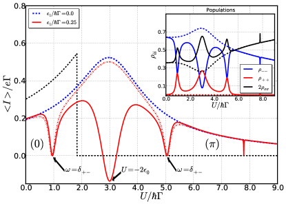
Figure 2: (Color online) Average current $\langle I\rangle$ as a function of Coulomb repulsion $U$. The black dashed curve results from the thermodynamic arguments in absence of driving. The full red (dashed blue) curve is the numerical solution of the Floquet master equation in presence (absence) of AC driving. The red dash-dotted curve is the outcome of the optical Bloch equations in the RWA approximation. Inset: The corresponding plain (dashed) numerical curves for the populations $\rho_{++},\rho_{--}$ and $2\rho_{\sigma\sigma}$ of the Andreev bound states in presence (absence) of AC driving. The parameters describing the Josephson junction are common to both plots: $\Delta/\hbar\Gamma=10.0,\epsilon_{0}/\hbar\Gamma=-1.5,\epsilon_{1}/\hbar\Gamma=0.25,\phi=\pi/2,\omega/\Gamma=2.5,k_{B}T_{EM}/\Delta=0,k_{B}T_{qp}/\Delta=1/20$ and $\gamma\Gamma^{2}=1.4\times 10^{-4}$.

Effect of driving.— An experimental way of testing the state of the junction is to irradiate the gate with an AC field. The resulting modulation in time of $\epsilon_{d}(t)$ is a perturbation that cannot change the parity of the junction. Since the odd-parity states are degenerate, the AC field can only induce resonant transitions between the even-parity states for small values of the detuning $\delta=\omega-\delta_{+-}$. Close to the resonance the dynamics can be described by performing a rotating-wave approximation that gives for the density matrix in the rotating frame $\tilde{\rho}_{a\bar{a}}=\rho_{a\bar{a}}e^{ia\omega t}$, $\tilde{\rho}_{aa}=\rho_{aa}$:

$$\dot{\tilde{\rho}}_{aa} = -i\frac{\Omega}{2}[\tilde{\rho}_{\bar{a}a}-\tilde{\rho}_{a\bar{a}}]$$

$$- (\Gamma_{a\bar{a}}+2\Gamma_{a\sigma})\tilde{\rho}_{aa}+\Gamma_{\bar{a}a}\tilde{\rho}_{\bar{a}\bar{a}}+2\Gamma_{\sigma a}\tilde{\rho}_{\sigma\sigma},$$

$$\dot{\tilde{\rho}}_{a\bar{a}} = -i\frac{\Omega}{2}[\tilde{\rho}_{\bar{a}\bar{a}}-\tilde{\rho}_{S;aa}]$$

$$+ [2ia\delta-(\Gamma_{a\bar{a}}+\Gamma_{\bar{a}a}+2\Gamma_{a\sigma}+2\Gamma_{\bar{a}\sigma})]\tilde{\rho}_{a\bar{a}}/2,$$

with $\tilde{\rho}_{\sigma\sigma}=(1-\tilde{\rho}_{++}-\tilde{\rho}_{--})/2$, $\tilde{\rho}_{\uparrow\downarrow}=\tilde{\rho}_{\downarrow\uparrow}\approx 0$, $\tilde{\rho}_{\bar{a}a}=\tilde{\rho}^{*}_{a\bar{a}}$ and $\hbar\Omega=\epsilon_{1}\sin(2\beta)$. As in the optical Bloch equations, when $\Omega\gg\Gamma_{+-},\Gamma_{a\sigma}$ the coherence terms are important for the time evolution of the system. The rates implying the quasi-particles are much smaller than all the other quantities appearing in the master equation. Using this fact one can solve the equations for the block $+/-$ for given $\rho_{\sigma\sigma}(t)$ and then solve separately the resulting equation for $\rho_{\sigma\sigma}$. This gives at vanishing $T_{EM}$:

$$\rho_{++}={\left[1+2\Gamma_{-\sigma}/\sum_{a}\Gamma_{\sigma a}\right]^{-1}(\Omega/2)^{2}\over\delta^{2}+\left(\Gamma_{+-}^{2}+\Omega^{2}(1+\theta)\right)/4}$$ (5)

with $\theta=(2\Gamma_{+\sigma}+\sum_{a}\Gamma_{\sigma a})/(2\Gamma_{-\sigma}+\sum_{a}\Gamma_{\sigma a})$, and $\rho_{++}/\rho_{--}=(\Omega/2)^{2}/[\delta^{2}+\left(\Gamma_{+-}^{2}+\Omega^{2}\right)/4]$. Eq. (5) describes a typical resonant behavior for the populations as it can be seen in the inset of Fig. 2. At resonance ($\delta=0$) the populations equilibrate so that $\rho_{++}=\rho_{--}=1-2\rho_{\sigma\sigma}=\sum_{a}\Gamma_{\sigma a}/2\sum_{a}(\Gamma_{a\sigma}+\Gamma_{\sigma a})$. Since typically the rates are of the same order of magnitude at resonance $\rho_{++}\approx 1/4$. The average current $\langle I\rangle$ is simply $\sum_{a}\rho_{aa}I_{aa}$ and it is strongly modulated near the resonances. The resonance is visible in both the regions where the 0- and $\pi$ phase would be stable. The narrow dip in Fig. 2 for $U/\hbar\Gamma\approx 8.0$ is a two-photon resonance described by the full numerical solution of Eq. (2).

The slow fluctuations between the $\sigma$ and $\pm$ doublets induce a strong telegraph noise, since the current in the four states is very different and the fluctuations are slow. To estimate the intensity of the current noise we assume that all current fluctuations are due to the transitions among the four states, each one having a different value for the stationary current (specifically $I_{++}=-I_{--}$, and $I_{\sigma\sigma}=0$). In absence of driving one finds that the current noise reads: $S=4\Gamma_{\sigma-}\Gamma_{-\sigma}I_{--}^{2}/(\Gamma_{\sigma-}+2\Gamma_{-\sigma})^{3}$, giving a very large Fano factor $F=S/2eI$ of the order of $e^{\Delta/k_{B}T_{\rm qp}}$. We note that a strong telegraph noise has been very recently observed in atomic point contact junctions Bretheau et al. (2013b). In that experiment the Coulomb blockade plays no role, but the coupling to the quasi-particles has a very similar behavior.

The driving reveals also an unexpected maximum of the population $\rho_{++}$ for $U=3\Gamma$. This is the value for which $2\epsilon_{0}+U=0$ and the $\left|0\right\rangle$ and $\left|2\right\rangle$ states are degenerate. At this point the matrix element entering the rate $\Gamma_{+-}$ vanishes. The population of the excited state generated by the non-resonant driving can relax to the $\left|-\right\rangle$ state only passing through the $\left|\sigma\right\rangle$ states, with very low rates. This allow a large population of the excited state with a consequent negative contribution to the supercurrent.

Conclusion.— We have investigated the effect of a coupling to the quasi-particles and the EM environment on the 0-$\pi$ transition. In a regime where the approximations can be well controlled we have shown that the quasi-particle scattering induces transitions between the $0$- and $\pi$- states, with a consequent washing out of the transition. We found that this induces large current fluctuations, and that the state of the junction could be investigated by driving the gate with an AC voltage. The main reason for the smoothening of the transition is the fact that the excess energy of the quasi-particles allows fluctuations from the thermodynamical ground state and the first excited state. This effect is very strong in the regime where we work, since $\Delta$ is the largest energy scale, but it will be present also for intermediate values of the gap. The theory we present indicates clearly that the effect of quasi-particles can be dramatic. The question of the crossover to the thermodynamical equilibrium when $\Delta$ is of the same order or smaller than the other energy scales remains open and calls for further investigations. The issue of the stability of Andreev bound states with respect to the quasi-particle scattering has also a strong relevance for the observation of Majorana states, that should be subject to a similar dynamics Fu and Kane (2009).

We acknowledge financial support from the ANR QNM $n^{\circ}$ 0404 01 and the PHC NANO ESPAGNE 2013 project $n^{\circ}$ 31404NA. Useful discussions with A. Levy Yeyati and D. G. Olivares are acknowledged. We thank for comments M. Houzet and M. F. Goffman.

References

- Kasumov et al. (1999) A. Y. Kasumov, R. Deblock, M. Kociak, B. Reulet, H. Bouchiat, I. I. Khodos, Y. B. Gorbatov, V. T. Volkov, C. Journet, and M. Burghard, Science 284, 1508 (1999).
- Steinbach et al. (2001) A. Steinbach, P. Joyez, A. Cottet, D. Esteve, M. H. Devoret, M. E. Huber, and J. M. Martinis, Phys. Rev. Lett. 87, 137003 (2001).
- Goffman et al. (2000) M. F. Goffman, R. Cron, A. Levy Yeyati, P. Joyez, M. H. Devoret, D. Esteve, and C. Urbina, Phys. Rev. Lett. 85, 170 (2000).
- van Dam et al. (2006) J. A. van Dam, Y. V. Nazarov, E. P. A. M. Bakkers, S. De Franceschi, and L. P. Kouwenhoven, Nature 442, 667 (2006).
- Pillet et al. (2010) J.-D. Pillet, C. H. L. Quay, P. Morfin, C. Bena, A. L. Yeyati, and P. Joyez, Nature Physics 6, 965 (2010).
- Deacon et al. (2010) R. S. Deacon, Y. Tanaka, A. Oiwa, R. Sakano, K. Yoshida, K. Shibata, K. Hirakawa, and S. Tarucha, Phys. Rev. Lett. 104, 076805 (2010).
- Basset et al. (2014) J. Basset, R. Delagrange, R. Weil, A. Kasumov, H. Bouchiat, and R. Deblock, (2014), arXiv:1403.4743 .
- Bulaevskii et al. (1977) L. Bulaevskii, V. Kuzii, and A. Sobyanin, JETP Lett 25, 290 (1977).
- Rozhkov et al. (2001) A. V. Rozhkov, D. P. Arovas, and F. Guinea, Phys. Rev. B 64, 233301 (2001).
- Buzdin (2005) A. I. Buzdin, Rev. Mod. Phys. 77, 935 (2005).
- Martín-Rodero and Levy Yeyati (2011) A. Martín-Rodero and A. Levy Yeyati, Advances in Physics 60, 899 (2011).
- Baselmans et al. (1999) J. J. A. Baselmans, A. F. Morpurgo, B. J. van Wees, and T. M. Klapwijk, Nature 397, 43 (1999).
- Ryazanov et al. (2001) V. V. Ryazanov, V. A. Oboznov, A. Y. Rusanov, A. V. Veretennikov, A. A. Golubov, and J. Aarts, Phys. Rev. Lett. 86, 2427 (2001).
- Kontos et al. (2002) T. Kontos, M. Aprili, J. Lesueur, F. Genet, B. Stephanidis, and R. Boursier, Phys. Rev. Lett. 89, 137007 (2002).
- Cleuziou et al. (2006) J.-P. Cleuziou, W. Wernsdorfer, V. Bouchiat, T. Ondarçuhu, and M. Monthioux, Nature Nanotechnology 1, 53 (2006).
- Jorgensen et al. (2007) H. I. Jorgensen, T. Novotny, K. Grove-Rasmussen, K. Flensberg, and P. E. Lindelof, Nano Letters 7, 2441 (2007).
- Eichler et al. (2009) A. Eichler, R. Deblock, M. Weiss, C. Karrasch, V. Meden, C. Schönenberger, and H. Bouchiat, Phys. Rev. B 79, 161407 (2009).
- Maurand et al. (2012) R. Maurand, T. Meng, E. Bonet, S. Florens, L. Marty, and W. Wernsdorfer, Phys. Rev. X 2, 011009 (2012).
- Pillet et al. (2013) J.-D. Pillet, P. Joyez, R. Žitko, and M. F. Goffman, Phys. Rev. B 88, 045101 (2013).
- Bretheau et al. (2013a) L. Bretheau, C. O. Girit, H. Pothier, D. Esteve, and C. Urbina, Nature 499, 312 (2013a).
- Bretheau et al. (2013b) L. Bretheau, C. O. Girit, C. Urbina, D. Esteve, and H. Pothier, Phys. Rev. X 3, 041034 (2013b).
- Ristè et al. (2013) D. Ristè, C. C. Bultink, M. J. Tiggelman, R. N. Schouten, K. W. Lehnert, and L. DiCarlo, Nature Communications 4, 1913 (2013).
- Olivares et al. (2014) D. G. Olivares, A. L. Yeyati, L. Bretheau, C. O. Girit, H. Pothier, and C. Urbina, Phys. Rev. B 89, 104504 (2014).
- Ingold and Nazarov (1992) G.-L. Ingold and Y. Nazarov, in Single Charge Tunneling, NATO ASI Series, Vol. 294, edited by H. Grabert and M. Devoret (Springer US, 1992) pp. 21–107.
- Glazman and Matveev (1989) L. Glazman and K. Matveev, JETP Lett 49, 659 (1989).
- Rozhkov and Arovas (1999) A. V. Rozhkov and D. P. Arovas, Phys. Rev. Lett. 82, 2788 (1999).
- Vecino et al. (2003) E. Vecino, A. Martín-Rodero, and A. Levy Yeyati, Phys. Rev. B 68, 035105 (2003).
- Benjamin et al. (2007) C. Benjamin, T. Jonckheere, A. Zazunov, and T. Martin, The European Physical Journal B 57, 279 (2007).
- Meng et al. (2009) T. Meng, S. Florens, and P. Simon, Phys. Rev. B 79, 224521 (2009).
- Yoshioka and Ohashi (2000) T. Yoshioka and Y. Ohashi, Journal of the Physical Society of Japan 69, 1812 (2000).
- Choi et al. (2004) M.-S. Choi, M. Lee, K. Kang, and W. Belzig, Phys. Rev. B 70, 020502 (2004).
- Siano and Egger (2004) F. Siano and R. Egger, Phys. Rev. Lett. 93, 047002 (2004).
- Cohen-Tannoudji et al. (1998) C. Cohen-Tannoudji, J. Dupont-Roc, and G. Grynberg, Atom-Photon Interactions: Basic Processes and Applications (Wiley, New York, 1998) p. 38.
- Grifoni and Hänggi (1998) M. Grifoni and P. Hänggi, Physics Reports 304, 229 (1998).
- Note (1) We estimated the low energy behavior of from Refs.Despósito and Levy Yeyati (2001); Bretheau et al. (2013a, b), involving a typical Josephson junction inductance , circuit resistance and superconducting gap .
- Fu and Kane (2009) L. Fu and C. L. Kane, Phys. Rev. B 79, 161408 (2009).
- Despósito and Levy Yeyati (2001) M. A. Despósito and A. Levy Yeyati, Phys. Rev. B 64, 140511 (2001).