Testing the mutual consistency of different supernovae surveys

Abstract

It is now common practice to constrain cosmological parameters using supernovae (SNe) catalogues constructed from several different surveys. Before performing such a joint analysis, however, one should check that parameter constraints derived from the individual SNe surveys that make up the catalogue are mutually consistent. We describe a statistically-robust mutual consistency test, which we calibrate using simulations, and apply it to each pairwise combination of the surveys making up, respectively, the UNION2 catalogue and the very recent JLA compilation by Betoule et al. We find no inconsistencies in the latter case, but conclusive evidence for inconsistency between some survey pairs in the UNION2 catalogue.

1 Introduction

Cosmology using type Ia supernovae (SNIa) has become a very successful and important field over the last 15 years, with SNIa playing a central role in the discovery of the accelerated expansion of the universe (Riess et al., 1998; Perlmutter et al., 1999). This accelerated expansion is broadly interpreted as an important piece of evidence for the existence of an exotic dark energy component. The basic approach assumes that SNIa constitute a set of ‘standardizable’ candles, since by applying small corrections to their absolute magnitudes, derived by fitting multi-wavelengths observations of their light-curves, one can reduce the scatter magnitude considerably, to around $\pm 0.15$ mag in the $B$-band (Phillips 1993; Hamuy et al. 1996). In essence, SNIa with broader light-curves and slower decline rates are intrinsically brighter than those with narrower light-curves and faster decline rates, similarly, bluer SNIa are intrinsically brighter than their redder counterparts (Tripp, 1998). Then, by measuring the distance moduli and redshifts of a set of SNIa, and comparing these with the predicted distance modulus for each SNIa, one can place constraints on the cosmological parameters.

From the very first such studies, SNIa from different telescopes have been combined in a joint analysis in order to have SNe both at low and high $z$ (Riess et al., 1998; Perlmutter et al., 1999). During the last few years, large combined SNe compilations (see e.g. Suzuki et al. 2012) are becoming widely used in SNe cosmology. Although such analyses result in tighter constraints on parameters, one needs to be careful when using data from different sources, as the presence of unaccounted systematics in any of these data-sets can lead to misleading results. Therefore, it is extremely important to establish whether different data-sets are consistent with each other before performing a joint analysis using them.

A common method to check for consistency between different data-sets, in general, is to perform a $\chi^{2}$ analysis and compare the best-fit values $\chi^{2}_{\rm min}$ obtained by using (i) all the data-sets together and (ii) each data-set independently. If the data-sets are mutually consistent, then one would expect that in each case $\chi^{2}_{\rm min}\sim N_{\rm dof}\pm\sqrt{2N_{\rm dof}}$, where $N_{\rm dof}$ is the number of degrees of freedom in the fit. It is, however, impossible to perform such a test in the standard framework of SNe analysis, since the intrinsic dispersion $\sigma_{\rm int}$, which describes the global variation in the SNIa absolute magnitudes that remains after correction for stretch and colour, is always adjusted so that a good fit is obtained (i.e. $\chi^{2}_{\rm min}\approx N_{\rm dof}$). Moreover, quite generally, tests based on $\chi^{2}_{\rm min}$ depend only on the best-fit values of parameters, and are insensitive to the likelihood over the rest of the parameter space.

One must therefore seek an alternative test for investigating consistency between different SNIa data-sets. Recently, Amendola et al. (2013); Heneka et al. (2014) carried out a search for systematic contamination within the UNION2.1 SNe catalogue (Suzuki et al., 2012) using a method based on the Bayesian consistency test described in Marshall et al. (2006). They concluded that UNION2.1 data do not suffer from significant systematic effects. Crucially, however, in this study some of the (non-cosmological) nuisance parameters were fixed, thereby eliminating by design any potential inconsistency arising from them.

The aim of this paper is to check for consistency between different SNe data-sets by using a statistically robust method, again based on the Bayesian test described in Marshall et al. (2006), but making as few assumptions as possible on the fitted parameters. This paper is organized as follows. We describe our analysis methodology including the details of our consistency test in Section 2. A short description of simulations and data we have used in this work is given in Section 3. Our results are given in Section 4. Finally, our conclusions are presented in Section 5.

2 Analysis methodology

SNIa survey data consist of the apparent magnitudes or fluxes observed in different filters, depending on the particular survey, at a series of epochs. Estimation of cosmological parameters from these flux measurements is a two-step procedure. First, a SN light-curve fitting algorithms is applied to these raw data in order to ‘standardise’ these observations by reducing the scatter in the Hubble diagram. Second, cosmological parameters are estimated using the output from the light-curve fitting method. In our analysis, this is followed by the application of a consistency test to the constraints derived both on the cosmological parameters and those associated with the SNe population.

2.1 Light-curve fitting

Standard algorithms for light-curve fitting include the Spectral Adaptive Light-curve Template method (SALT) (Guy et al., 2005; Astier et al., 2006), SALT-II (Guy et al., 2010), SiFTO (Conley et al., 2008), Multi Colour light-curve Shape (MLCS) method (Jha et al., 2007), Gaussian Process Data Regression (Kim et al., 2013), and Hierarchical Models (Mandel et al., 2011). In this paper we employ the SALT-II SN light-curve fitter, since it was used to obtain the data-sets described in Section 3.1.

When fitting SN light-curves with SALT-II, the outputs are the best-fit values $\hat{m}_{B}^{\ast}$ of the apparent rest frame $B$-band magnitudes of the SNe at maximum luminosity, the light-curve shape parameter $\hat{x}_{1}$ related to the width (stretch) of the fitted light-curve, the colour $\hat{c}$ in the $B$-band at maximum luminosity, and the covariance matrix of the uncertainties in the estimated light-curve parameters

$$\widehat{C}=\left(\begin{array}[]{ccc}\sigma^{2}_{m^{\ast}_{B}}&\sigma_{m^{\ast}_{B},x_{1}}&\sigma_{m^{\ast}_{B},c}\\[5.69054pt] \sigma_{m^{\ast}_{B},x_{1}}&\sigma^{2}_{x_{1}}&\sigma_{x_{1},c}\\[5.69054pt] \sigma_{m^{\ast}_{B},c}&\sigma_{x_{1},c}&\sigma^{2}_{c}\\ \end{array}\right).$$ (1)

Combining these quantities with the estimated redshift $\hat{z}$ of the SN, our basic input data for each SN are thus

$$D_{i}\equiv\{\hat{z}_{i},\hat{m}_{B,i}^{\ast},\hat{x}_{1,i},\hat{c}_{i}\}$$ (2)

for ($i=1,\ldots,N_{\rm SN}$). The vector of values $(\hat{m}_{B,i}^{\ast},\hat{x}_{1,i},\hat{c}_{i})$ for each SN is then assumed to be distributed as a multivariate Gaussian about their respective true values, with covariance matrix $\widehat{C}_{i}$.

2.2 Parameter estimation

The output from the light-curve fitting constitutes the data used to estimate parameters, both cosmological and those associated with the SNe population. The usual way in which this analysis is performed by the SNe community is to use the standard $\chi^{2}$-method, see for example Astier et al. (2006); Kessler et al. (2009); Guy et al. (2010). Recently, other inference methods have been proposed, such as a likelihood approach by Lago et al. (2012) and the Bayesian Hierarchical Method (BHM; March et al. 2011, 2012), both of which are better motivated statistically than the standard $\chi^{2}$ analysis. Nonetheless, in this paper we employ the $\chi^{2}$ method, since it remains the approach most commonly used by the SNe community.

In this approach, the $\chi^{2}$ misfit function is defined to be

$$\chi^{2}(\mathscr{C},\alpha,\beta,M_{0},\sigma_{\text{int}})=\sum_{i=1}^{N}\frac{[\mu_{i}^{\text{obs}}(\alpha,\beta,M_{0})-\mu(\hat{z}_{i},\mathscr{C})]^{2}}{\sigma_{i}^{2}(\alpha,\beta,\sigma_{\text{int}})},$$ (3)

where, for clarity, we have made explicit the functional dependencies of the various terms on (only) the parameters to be fitted. In this expression, the ‘observed’ distance modulus for the $i$th SN is

$$\mu_{i}^{\rm obs}=\hat{m}_{B,i}^{\ast}-M_{0}+\alpha\hat{x}_{1,i}-\beta\hat{c}_{i},$$ (4)

where $M_{0}$ is the (unknown) $B$-band absolute magnitude of the SNe, and $\alpha$, $\beta$ are (unknown) nuisance parameters controlling the stretch and colour corrections; all three parameters are assumed to be global, i.e. the same for all SNIa. The predicted distance modulus is given by

$$\mu(z,\mathscr{C})=5\log_{10}\left[\frac{D_{L}(z,\mathscr{C})}{\text{Mpc}}\right]+25,$$ (5)

where $D_{L}(z,\mathscr{C})$ is the luminosity distance to an object of redshift $z$ in a universe with cosmological parameters $\mathscr{C}=\{\Omega_{m,0},\Omega_{\Lambda,0},H_{0},w\}$. The total dispersion $\sigma_{i}^{2}$ is the sum of several errors added in quadrature:

$$\sigma_{i}^{2}=(\sigma_{\mu,i}^{z})^{2}+\sigma_{\text{int}}^{2}+\sigma_{\text{fit},i}^{2}(\alpha,\beta).$$ (6)

The three components are: (i) the error $\sigma_{\mu,i}^{z}$ in the distance modulus that is induced by the error $\sigma_{z,i}$ in the redshift measurement, which may be due to uncertainties in the peculiar velocity of the host galaxy or SNIa and in the spectroscopic measurements of either the host galaxy of the SNIa itself; (ii) the intrinsic dispersion $\sigma_{\text{int}}$, which describes the global variation in the SNIa absolute magnitudes that remain after correction for stretch and colour, which quantifies all of the unknown intrinsic dispersion errors; and (iii) the fitting error, which is given by

$$\sigma_{\text{fit},i}^{2}(\alpha,\beta)=\mn@boldsymbol{\psi}^{\rm t}\widehat{C}_{i}\mn@boldsymbol{\psi},$$ (7)

where the transposed vector $\mn@boldsymbol{\psi}^{\rm t}=\left(1,\alpha,-\beta\right)$ and $\widehat{C}_{i}$ is the covariance matrix given in (1).

Typically, the chi-squared function (3) is minimized simultaneously with respect to the cosmological parameters $\mathscr{C}$ and the global SNIa nuisance parameters $M_{0}$, $\alpha$ and $\beta$, with $\sigma_{\text{int}}$ fixed to some initial estimate. There are, however, a few differences in the way in which this minimisation is performed, such as which search algorithm is used (MCMC techniques or grid searches) and the treatment of $M_{0}$ (which is degenerate with $H_{0}$), in particular whether this parameter is marginalised over analytically or numerically. Once the minimum value of chi-squared has been obtained, the value of $\sigma_{\text{int}}$ is updated by adjusting it to obtain $\chi^{2}_{\rm min}/N_{\rm dof}\sim 1$; the entire process may be iterated, if necessary, until $\sigma_{\text{int}}$ converges.

In this paper, we accommodate the exact degeneracy between $M_{0}$ and $H_{0}$ by fixing $H_{0}=73$ km s^-1 Mpc^-1, which is consistent with independent constraints from other probes Planck Collaboration et al. (2013), and allow $M_{0}$ to vary. For simplicity, we also assume that dark energy is in the form of a cosmological constant $(w=-1)$ and that the universe is spatially-flat $(\Omega_{\Lambda,0}+\Omega_{\text{m},0}=1)$; thus we vary only the parameters $\{\Omega_{\text{m},0},M_{0},\alpha,\beta,\sigma_{\text{int}}\}$. In keeping with standard practice, we define the ‘likelihood’ to be simply

$$\mathcal{L}(\Omega_{\text{m},0},M_{0},\alpha,\beta,\sigma_{\text{int}})=\exp[-\tfrac{1}{2}\chi^{2}(\Omega_{\text{m},0},M_{0},\alpha,\beta,\sigma_{\text{int}})]$$ (8)

which is clearly not properly normalized. More importantly, this ‘likelihood’ is not (proportional to) the probability $\Pr(\mn@boldsymbol{D}|\Omega_{\text{m},0},M_{0},\alpha,\beta,\sigma_{\text{int}})$. Statistically well-motivated expressions for the latter may be found using the likelihood or BHM approaches mentioned above, but we will not pursue such methods here.

Adopting the initial value $\sigma_{\text{int}}=0.1$, we use the nested sampling algorithm MultiNest (Feroz & Hobson, 2008; Feroz et al., 2009; Feroz et al., 2013) to sample from the (unnormalised) ‘posterior’ $\mathcal{P}(\mathbf{\Theta},\sigma_{\text{int}})=\mathcal{L}(\mathbf{\Theta},\sigma_{\text{int}})\pi(\mathbf{\Theta})$ over the parameter space $\mathbf{\Theta}=\{\Omega_{\text{m},0},M_{0},\alpha,\beta\}$, assuming the separable, uniform priors $\pi(\mathbf{\Theta})$ listed in Table 1. Following the standard approach, the value of $\sigma_{\text{int}}$ is estimated by adjusting it to obtain $\chi^{2}_{\rm min}/N_{\rm dof}\sim 1$, where $\chi^{2}_{\rm min}$ is the value at the maximum $\widehat{\mathbf{\Theta}}$ of the ‘posterior’ (and also of the ‘likelihood’, since the assumed priors are uniform). The sampling over the parameter space $\mathbf{\Theta}$ is then repeated. We find that one or two such iteration on $\sigma_{\text{int}}$ is sufficient to achieve convergence.

Parameter	Symbol	Prior	Simulated value
Matter density	$\Omega_{\text{m},0}$	${\cal U}(0,1)$	0.3
Absolute magnitude	$M_{0}$	${\cal U}(-20.3,-18.3)$	$-19.3$
Stretch multiplier	$\alpha$	${\cal U}(0,1)$	0.12
Colour multiplier	$\beta$	${\cal U}(1,5)$	2.6

Table 1: Priors assumed on the parameters, where $U(a,b)$ indicates the uniform distribution in the range $[a,b]$. The final column gives the value assumed in generating the simulated data.

We note that, when jointly analysing a full catalogue of SNIa data, $\sigma_{\text{int}}$ is the same for all SNe, regardless of whether they belong to the same survey or not. Apart from modelling the intrinsic dispersion in distance moduli of SNe, however, $\sigma_{\text{int}}$ can also account for systematics in different surveys. Therefore different surveys are allowed to have different values of $\sigma_{\text{int}}$ when analysing them separately.

2.3 Test for mutual consistency between data-sets

The standard approach to analysing multiple data-sets jointly is simply to assume that they are mutually consistent. We represent this (null) hypothesis by $H_{0}$. This is the approach adopted in the vast majority of analyses in SNe cosmology. It may be the case, however, that the data-sets are inconsistent with one another, resulting in each one favouring a different region of the model parameter space. We represent this (alternative) hypothesis by $H_{1}$. In this case, a joint analysis would lead to completely misleading results (see, for example, Appendix A in Feroz et al. 2008 for a demonstration).

In order to determine which one of these hypotheses is favoured by the data, one can perform Bayesian model selection between $H_{0}$ and $H_{1}$. Assuming that hypothesis $H_{0}$ and $H_{1}$ are equally likely a priori, this can be achieved by calculating the ratio

$$\mathcal{R}=\frac{\Pr(\mathbf{D}|H_{0})}{\Pr(\mathbf{D}|H_{1})}=\frac{\Pr(\mathbf{D}|H_{0})}{\prod_{i}\Pr(D_{\rm i}|H_{1})}.$$ (9)

where the probabilities $\Pr(\mathbf{D}|H)$, called Bayesian evidences or marginal likelihoods, are defined as

$$\Pr(\mathbf{D}|H)=\int{\Pr(\mathbf{D}|\mathbf{\Theta},H)\Pr(\mathbf{\Theta}|H)}\mathrm{d}^{n}\mathbf{\Theta}.$$ (10)

Here $n$ is the dimensionality of the parameter space, $\Pr(\mathbf{D}|\mathbf{\Theta},H)$ is the likelihood and $\Pr(\mathbf{\Theta}|H)$ is the prior. The numerator of (9) represents the standard joint analysis of all the data-sets $\mathbf{D}=\{D_{1},D_{2},\cdots,D_{n}\}$, whereas the denominator in the final expression represents the case in which each data-set is analysed separately It is worth noting, however, that the second equality in (9) is valid only when one allows for potential inconsistencies in the preferred values of the full set of model parameters $\mathbf{\Theta}$.

In adapting this Bayesian test to apply it to the standard $\chi^{2}$ analysis of SNIa data, $\Pr(\mathbf{D}|\mathbf{\Theta},H)$ is replaced by the ‘likelihood’ $\mathcal{L}(\mathbf{\Theta},\sigma_{\text{int}})$ given in (8) and $\Pr(\mathbf{\Theta}|H)$ by the prior $\pi(\mathbf{\Theta})$ listed in Table 1. In so doing, however, the terms in (9) can not be interpreted directly as probabilities, and thus the value of the $\mathcal{R}$ cannot be compared with the normal Jeffrey’s scale for model selection based on the ratio of evidences. Nonetheless, $\mathcal{R}$ values are still expected to be higher for consistent data-sets and lower for inconsistent ones (March et al., 2011), so $\mathcal{R}$ may be used as a test statistic that is ‘calibrated’ with simulations to perform a standard one-sided frequentist hypothesis test.

Thus, we construct the distribution of $\mathcal{R}$ under the null hypothesis $H_{0}$ by evaluating it for a large set of simulations in which the individual surveys making up a catalogue are mutually consistent. The $\mathcal{R}$ value obtained by analysing the real data can then be used to calculate the $p$-value as follows:

$$p=\frac{N(\mathcal{R}_{\rm s}<\mathcal{R}_{\rm r})}{N_{\rm tot}},$$ (11)

where $\mathcal{R}_{\rm s}$ and $\mathcal{R}_{\rm r}$ are the $\mathcal{R}$ values obtained by analysing simulated and real data-sets respectively, $N(\mathcal{R}_{\rm s}<\mathcal{R}_{\rm r})$ is the number of simulations with $\mathcal{R}$ values less than that obtained by analysing the real data and $N_{\rm tot}$ is the total number of simulations. We use the scale given in Table 2 to draw inferences from these $p$-values about the mutual consistency of the data-sets

$p$-value	Conclusion
$<0.01$	very strong presumption against $H_{0}$
$0.01-0.05$	strong presumption against $H_{0}$
$0.05-0.10$	low presumption against $H_{0}$
$>0.10$	no presumption against $H_{0}$

Table 2: Thresholds for the $p$-value.

3 Data-sets

3.1 Real data

In this paper we consider SNe from the UNION2 catalogue (Amanullah et al., 2010) and the ‘joint light-curve analysis’ (JLA) compilation given in Betoule et al. (2014). These data-sets consist of SNe observed by different telescopes. Since our aim in this paper is to check for consistency between different SNe surveys/data-sets, we divide these SNe according to the telescope with which they have been observed. In particular, we divide SNe into the following subsets: ESSENCE (Miknaitis et al., 2007; Wood-Vasey et al., 2007; Krisciunas et al., 2005), Hubble Space Telescope (HST; Garnavich et al. 1998; Knop et al. 2003; Riess et al. 2004, 2007), Sloan Digital Sky Survey (SDSS; Frieman et al. 2008; Kessler et al. 2009; Holtzman et al. 2008; Betoule et al. 2014), Supernova Legacy Survey (SNLS; Astier et al. 2006; Guy et al. 2010 , S11), CfA (Hicken et al. 2009a) and a compilation of nearby SNIa measurements (Hamuy et al. 1996; Riess et al. 1999; Contreras et al. 2010; Jha et al. 2006). Even though the SNe in the nearby compilation have not all been observed from the same telescope, we treat them as if they were. This is normal practice in SN analyses, and is justified since such SNe are usually observed with similar precision and sets of filters. The resulting number of SNe in the UNION2 and JLA compilations coming from each of the subsets is given in Table 3. These corresponds to all the SNe in the JLA compilation, but does exclude some SNe from the UNION2 catalogue, which were observed by telescopes contributing just a handful of SNe in each case.

Data-set	UNION2	JLA
ESSENCE	74	—
HST	42	9
SDSS	131	374
SNLS	72	239
CfA	100	—
Low-$z$	—	118
$\left(\mbox{Total}\right.$	419	$\left.740\right)$

Table 3: Number of SNe in the UNION2 and JLA compilations coming from each survey. Note that the CfA survey in the UNION2 compilation and the low-$z$ survey in the JLA compilation have 51 SNe in common.

We use the publically-available fitted values of $\hat{m}_{B}^{\ast}$, $\hat{x}_{1}$, $\hat{c}$ and $\widehat{C}$ from SALT-II light-curve fits and the estimated redshifts $\hat{z}$ listed in the UNION2 and JLA catalogues. For the JLA catalogue, however, we note that the quoted covariance matrix $\widehat{C}$, in particular the element $\sigma^{2}_{m_{B}^{\ast}}$, also contains the three variances listed on the right-hand side of (6). To treat the UNION2 and JLA catalogues in a consistent manner, we therefore subtracted these contributions from $\sigma^{2}_{m_{B}^{\ast}}$ before analysing the JLA catalogue. We do not apply any additional cuts to the ones that have already been applied to these catalogues. We refer readers to papers describing these catalogues Amanullah et al. (2010); Betoule et al. (2014) for details on how the SNe have been corrected for galactic extinction, peculiar velocities (at low z), Malmquist and other selection biases.

3.2 SNANA simulations

In order to calibrate our test statistic $\mathcal{R}$ and calculate the resultant $p$-values, as described in Sec. 2, we simulate SNe using the publicly available SNANA package (Kessler et al., 2009). SNANA has a two-step simulation process. First, data were simulated using appropriate light-curve simulation templates to match the real data-sets closely. The second stage is the light-curve fitting process in which the photometric data are fitted to SALT II templates to give estimates for $D_{i}\equiv\{\hat{z}_{i},\hat{m}_{B,i}^{\ast},\hat{x}_{1,i},\hat{c}_{i}\}$. At this light-curve fitting stage, basic cuts are made to discard SNIa with a low signal-to-noise ratio and/or too few observed epochs in sufficient bands. After the light-curve fitting stage we make a redshift dependent magnitude correction for the Malmquist bias; the correction is taken from a spline interpolation of Table 4 in Perrett et al. (2010). All selection cuts and Malmquist corrections are made prior to the cosmology inference step.

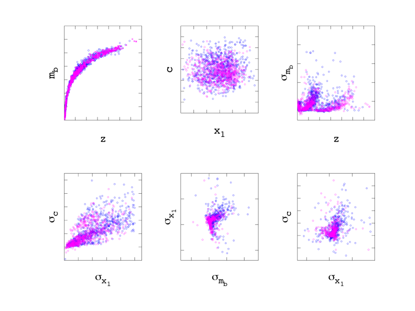
Figure 1: A simulated SNANA data-set (blue points) and real data from the JLA compilation (pink points).

Our null hypothesis $H_{0}$ is that different data-sets are consistent with each other. Therefore, we simulate all data-sets with exactly the same parameter values, which are listed in Table 1, and an intrinsic dispersion $\sigma_{\text{int}}=0.106$. For the UNION2 and JLA compilations, respectively, 100 data-sets were simulated for each telescope/survey, with the numbers of SNe matching those listed in Table 3. Fig. 1 shows a compilation of one set of simulations, chosen at random, for each telescope in the JLA compilation, overplotted on the real JLA data. A similar level of agreement between simulations and real data is obtained for the UNION2 catalogue.

4 Results

4.1 Constraints on $\Omega_{\rm m,0}$ and $M_{0}$

In analysing compilations of SNe data, it is usual simply to plot the combined constraints on cosmological parameters obtained from a full joint analysis. Here we begin by instead calculating the constraints imposed by each constituent survey in the UNION2 and JLA compilations, respectively. The resulting two-dimensional marginalised constraints on the parameters $(\Omega_{\rm m,0},M_{0})$ are shown in Figs 2 and 3. We recall that $M_{0}$ is exactly degenerate with $H_{0}$, and so we have fixed the latter to $H_{0}=73$ km s^-1 Mpc^-1, in accordance with values obtained from independent probes.

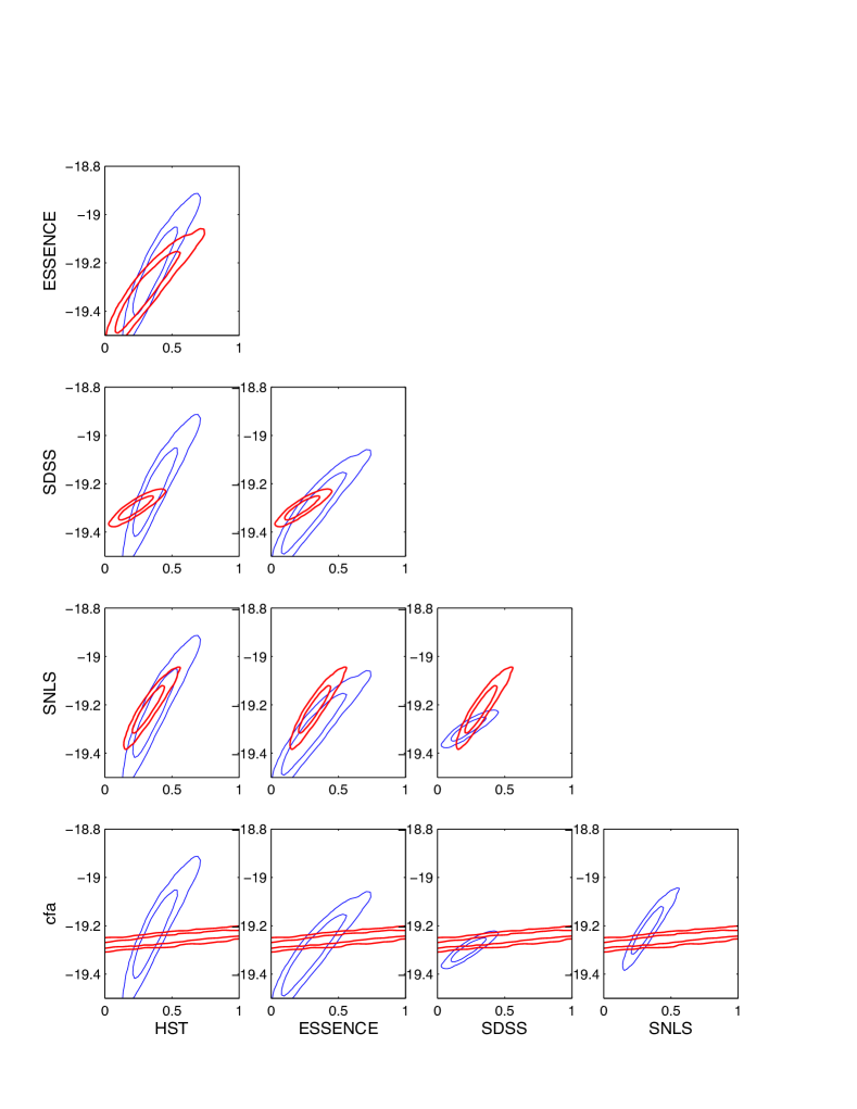
Figure 2: Two-dimensional marginalised constraints on the parameters $(\Omega_{\rm m,0},M_{0})$ obtained from the individual constituent surveys contained in the UNION2 catalogue. The red (blue) contours denote the 68 and 95 per cent confidence regions for the survey in that row (column).

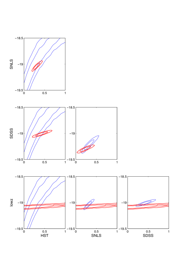
Figure 3: As in Fig. 2, but for the JLA compilation.

Figure 4: Two-dimensional marginalised constraints on the parameters $(\alpha,\beta)$ obtained from the individual constituent surveys contained in the UNION2 catalogue. The red (blue) contours denote the 68 and 95 per cent confidence regions for the survey in that row (column).

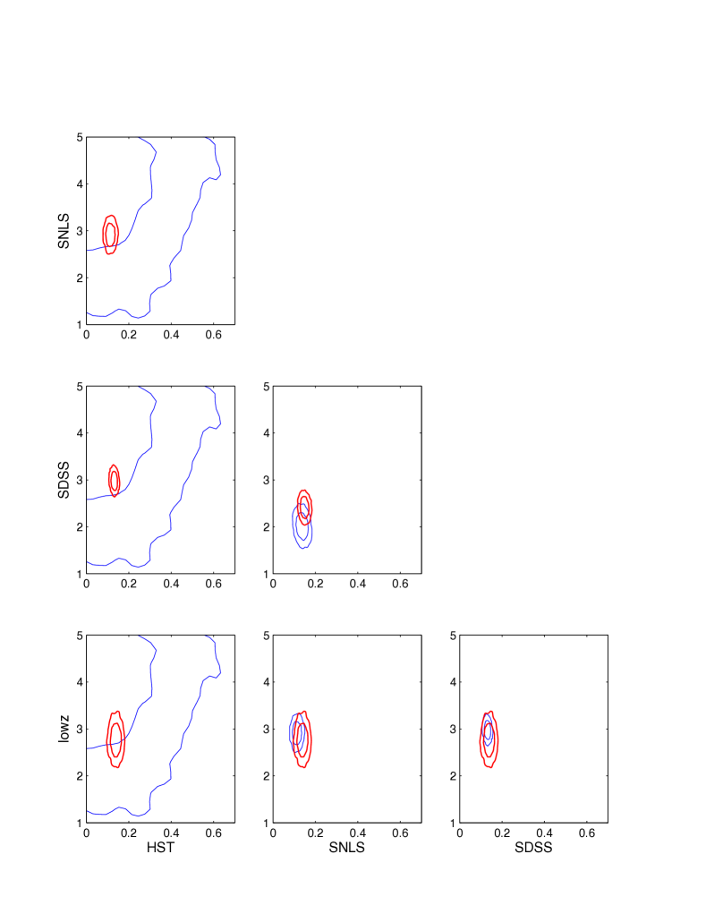
Figure 5: As in Fig. 4, but for the JLA compilation.

For the UNION2 compilation, the tightest constraints are produced by the SDSS and SNLS surveys, with ESSENCE providing somewhat weaker constraints. As might be expected, the CfA survey alone constrains the parameters rather poorly, since it consists only of nearby SNe. For the JLA compilation, the SDSS and SNLS surveys again provide the tightest constraints, with the HST and low-$z$ surveys constraining the parameters only very weakly, as one would expect. For both compilations, however, the key observation for our purposes is that the constraints from the constituent surveys are in good agreement, as indicated by the large degree of overlap of the confidence contours for each pairwise comparison.

4.2 Constraints on $\alpha$ and $\beta$

We now consider the constraints on the stretch and colour corrections multipliers $\alpha$ and $\beta$, which are not often presented in the analysis of SNe data. Once again we calculate the constraints imposed by each constituent survey in the UNION2 and JLA compilations, respectively. The resulting two-dimensional marginalised constraints on the parameters $(\alpha,\beta)$ are shown in Figs 4 and 5.

For the UNION2 compilation, the tightest constraints are produced by the CfA survey, with the remaining surveys yielding weaker constraints all of a similar quality. It can be seen, however, that for several pairings the confidence contours for the two surveys are significantly displaced from one another, and do not overlap at all in some cases. This indicates mutual inconsistency between the survey pairs and is most notable for CfA/SNLS, CfA/SDSS, SNLS/HST, SNLS/ESSENCE and SDSS/HST. For the JLA compilation, the low-$z$, SDSS and SNLS surveys all provide constraints of a similar quality, whereas the HST constraints are very weak, as one might expect since this corresponds to just 9 SNe. The key observation, however, is that for each pairing the confidence contours for the two surveys overlap well, indicating mutual consistency, in sharp contrast to the UNION2 results.

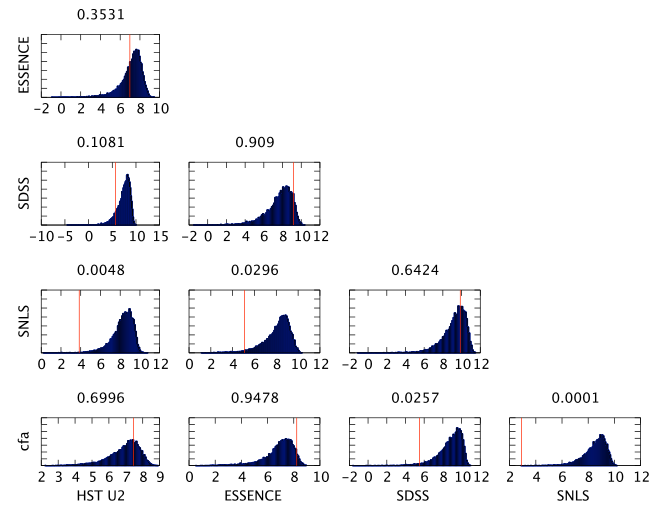
Figure 6: Results of the consistency test applied to surveys pairs in the UNION2 compilation. The blue histograms show the distribution of $R$ values obtained from $10^{4}$ consistent simulations of each pair, and the red vertical line indicates the $R$ value obtained from the real data. The corresponding one-sided $p$-value is given above each panel.

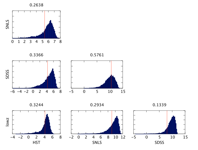
Figure 7: As in Fig. 6, but for the JLA compilation.

4.3 Mutual consistency test between survey pairs

To quantify the level of mutual (in)consistency between survey pairs in the UNION2 and JLA compilations, respectively, we calculate our test statistic $\mathcal{R}$ for each combination, and compare it with the distribution of $\mathcal{R}$ values for the corresponding survey pair obtained from our consistent simulations. Since we generated 100 simulations for each survey, we have $10^{4}$ simulated pairs in each case.

The results of the consistency test for the UNION2 compilation are shown in Fig. 6, together with the corresponding $p$-values. It is clear that the $p$-values obtained agree very closely with the degree of overlap between the confidence contours plotted in Fig. 4. In particular, we find very strong evidence, at more than the 99 per cent significance level, for inconsistency between the survey pairs CfA/SNLS and SNLS/HST. We also find strong evidence, at more than 95 per cent significance, for inconsistency in the pairs CfA/SDSS and SNLS/ESSENCE.

The results obtained for the JLA compilation are shown in Fig. 7 It can be seen that none of the survey pairs shows evidence for inconsistency, even at the 90 per cent significance level, which is in agreement with the good degree of overlap between the confidence contours plotted in Fig. 5.

The consistency between the survey pairs in the JLA compilation is in sharp contrast to inconsistencies present the UNION2 compilation. This difference must result from the different SNe selection criteria and calibration techniques used in the construction of the two compilations.

4.4 Effect of selection cuts on mutual consistency

We now investigate the effect of selection cuts on two of the most mutually inconsistent survey pairs within the UNION2 compilation, namely CfA/SNLS and CfA/SDSS. To this end, we divide the 100 SNe in the CfA data-set contained within UNION2 into two subsets of equal size. The first subset (CfA-1) consists of 50 SNe chosen at random from the 51 that are also present within the low-$z$ survey contained in the JLA catalogue, and the second subset (CfA-2) consists of the remaining 50 SNe in the CfA data-set. Clearly, all but one of the SNe in CfA-2 are not present in the JLA catalogue. We then quantify the level of mutual (in)consistency between each of these subsets and the SNLS and SDSS surveys, respectively, in precisely the same manner as in Section 4.3.

The results are shown in Figs 8 and 9. It is clear that the CfA-1 subsurvey is consistent with both the SNLS and SDSS surveys, whereas the CfA-2 subsurvey is inconsistent at very high significance in both cases. This suggests that it is the selection of appropriate SNe, and not necessarily the improved fitting method, that is key to achieving the mutual consistency of the surveys within the JLA compilation

5 Conclusions

SNe are now routinely used to constrain cosmological parameters, in combination with CMB and large-scale structure observations. SNe catalogues typically consist of SNe from a number of different surveys, and most studies perform a joint analysis of all the surveys within a given SNe catalogue. A key (often implicit) assumption underlying these joint analyses is that the different SNe surveys that make up the catalogue are mutually consistent. It is possible, however, that unaccounted for systematics may cause tensions or even inconsistencies in the parameters preferred by some surveys comprising the catalogue. It is therefore extremely important to establish whether any such inconsistencies exist before performing a joint analysis.

In this paper we have performed a robust statistical test to look for inconsistencies among the different surveys making up the UNION2 and JLA catalogues, respectively. The test is based on a Bayesian prescription, but has been adapted to be applied to analyses performed using the standard $\chi^{2}$ analysis that is used most widely by the SNe community. Our main finding is that, although the cosmological constraints derived from the different surveys making up the UNION2 and JLA catalogues are consistent, the constraints on the parameters associated with the SNe population, namely the multipliers $\alpha$ and $\beta$ of the stretch and colour corrections respectively, are significantly different for the UNION2 catalogue, but consistent for the JLA catalogue. The level of inconsistency exhibited by the UNION2 compilation suggests that one must exercise caution when interpreting cosmological constraints derived from it with the usual joint analysis.

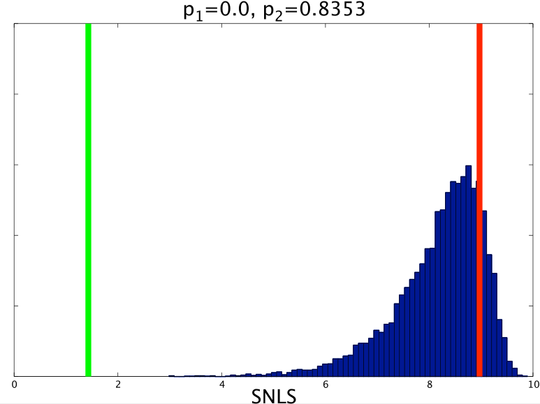
Figure 8: Results of the consistency test applied to the pairs CfA-1/SNLS (red vertical line) and CfA-2/SNLS (green vertical line) from the UNION2 compilation. The blue histogram shows the distribution of $R$ values obtained from consistent simulations of the (sub)surveys. The corresponding one-sided $p$-values are also given.

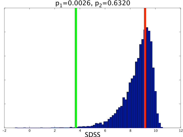
Figure 9: As in Fig. 8, but for the pairs CfA-1/SDSS and CfA-2/SDSS.

References

- Amanullah et al. (2010) Amanullah R., et al., 2010, ApJ, 716, 712
- Amendola et al. (2013) Amendola L., Marra V., Quartin M., 2013, MNRAS, p. 694
- Astier et al. (2006) Astier P., et al., 2006, A&A, 447, 31
- Astier et al. (2006) Astier P., Guy J., Regnault N., Pain R., Aubourg E., Balam D., Basa S., Carlberg R. G., Fabbro S., 2006, A&A, 447, 31
- Betoule et al. (2014) Betoule M., et al., 2014, ArXiv e-prints
- Conley et al. (2008) Conley A., Sullivan M., Hsiao E. Y., Guy J., Astier P., Balam D., Balland C., Basa S., Carlberg R. G., Fouchez D., Hardin D., Howell D. A., Hook I. M., Pain R., Perrett K., Pritchet C. J., Regnault N., 2008, ApJ, 681, 482
- Contreras et al. (2010) Contreras C., et al., 2010, AJ, 139, 519
- Feroz et al. (2008) Feroz F., Allanach B. C., Hobson M., Abdus Salam S. S., Trotta R., Weber A. M., 2008, Journal of High Energy Physics, 10, 64
- Feroz & Hobson (2008) Feroz F., Hobson M. P., 2008, MNRAS, 384, 449
- Feroz et al. (2009) Feroz F., Hobson M. P., Bridges M., 2009, MNRAS, 398, 1601
- Feroz et al. (2013) Feroz F., Hobson M. P., Cameron E., Pettitt A. N., 2013, ArXiv e-prints
- Frieman et al. (2008) Frieman J. A., et al., 2008, AJ, 135, 338
- Garnavich et al. (1998) Garnavich P. M., et al., 1998, ApJ, 493, L53
- Guy et al. (2005) Guy J., Astier P., Nobili S., Regnault N., Pain R., 2005, A&A, 443, 781
- Guy et al. (2010) Guy J., et al., 2010, A&A, 523, A7
- Guy et al. (2010) Guy J., Sullivan M., Conley A., Regnault N., Astier P., Balland C., Basa S., Carlberg R. G., Fouchez D., Hardin D., Hook I. M., Howell D. A., Pain R., 2010, aap, 523, A7
- Hamuy et al. (1996) Hamuy M., et al., 1996, AJ, 112, 2408
- Hamuy et al. (1996) Hamuy M., Phillips M. M., Suntzeff N. B., Schommer R. A., Maza J., Aviles R., 1996, AJ, 112, 2391
- Heneka et al. (2014) Heneka C., Marra V., Amendola L., 2014, MNRAS, 439, 1855
- Hicken et al. (2009a) Hicken M., et al., 2009a, ApJ, 700, 331
- Hicken et al. (2009b) Hicken M., et al., 2009b, Astrophys. J., 700, 331
- Holtzman et al. (2008) Holtzman J. A., et al., 2008, AJ, 136, 2306
- Holtzman et al. (2008) Holtzman J. A., Marriner J., Kessler R., Sako M., Dilday B., Frieman J. A., Schneider D. P., Bassett B., Becker A., Cinabro D., DeJongh F., Depoy D. L., Doi 2008, AJ, 136, 2306
- Jha et al. (2006) Jha S., et al., 2006, AJ, 131, 527
- Jha et al. (2007) Jha S., Riess A. G., Kirshner R. P., 2007, Astrophys. J., 659, 122
- Kessler et al. (2009) Kessler R., et al., 2009, Astrophys. J. S., 185, 32
- Kessler et al. (2009) Kessler R., et al., 2009, ApJS, 185, 32
- Kessler et al. (2009) Kessler R., et al., 2009, arXiv:0908.4280
- Kim et al. (2013) Kim A. G., et al., 2013, ApJ, 766, 84
- Knop et al. (2003) Knop R. A., et al., 2003, ApJ, 598, 102
- Krisciunas et al. (2005) Krisciunas K., et al., 2005, AJ, 130, 2453
- Lago et al. (2012) Lago B. L., Calvão M. O., Jorás S. E., Reis R. R. R., Waga I., Giostri R., 2012, A&A, 541, A110
- Lampeitl et al. (2009) Lampeitl H., Nichol R. C., Seo H. J., Giannantonio T., Shapiro C., Bassett 2009
- Mandel et al. (2011) Mandel K. S., Narayan G., Kirshner R. P., 2011, ApJ, 731, 120
- March et al. (2012) March M. C., Karpenka N. V., Feroz F., Hobson M. P., 2012, ArXiv e-prints
- March et al. (2011) March M. C., Trotta R., Amendola L., Huterer D., 2011, MNRAS, 415, 143
- March et al. (2011) March M. C., Trotta R., Berkes P., Starkman G. D., Vaudrevange P. M., 2011, MNRAS, 418, 2308
- Marshall et al. (2006) Marshall P., Rajguru N., Slosar A., 2006, Phys.Rev.D, 73, 067302
- Miknaitis et al. (2007) Miknaitis G., et al., 2007, ApJ, 666, 674
- Perlmutter et al. (1999) Perlmutter S., et al., 1999, ApJ, 517, 565
- Perrett et al. (2010) Perrett K., Balam D., Sullivan M., Pritchet C., Conley A., Carlberg R., Astier P., Balland C., Basa S., Fouchez D., Guy J., Hardin D., Hook I. M., Howell D. A., Pain R., Regnault N., 2010, aj, 140, 518
- Phillips (1993) Phillips M. M., 1993, ApJ, 413, L105
- Planck Collaboration et al. (2013) Planck Collaboration Ade P. A. R., Aghanim N., Alves M. I. R., Armitage-Caplan C., Arnaud M., Ashdown M., Atrio-Barandela F., Aumont J., Aussel H., et al. 2013, ArXiv e-prints
- Riess et al. (1998) Riess A. G., et al., 1998, AJ, 116, 1009
- Riess et al. (1999) Riess A. G., et al., 1999, AJ, 117, 707
- Riess et al. (2004) Riess A. G., et al., 2004, ApJ, 607, 665
- Riess et al. (2007) Riess A. G., et al., 2007, ApJ, 659, 98
- Strolger & Riess (2006) Strolger L.-G., Riess A. G., 2006, AJ, 131, 1629
- Suzuki et al. (2012) Suzuki N., et al., 2012, ApJ, 746, 85
- Tripp (1998) Tripp R., 1998, A&A, 331, 815
- Wood-Vasey et al. (2007) Wood-Vasey W. M., et al., 2007, ApJ, 666, 694