Wind Finslerian structures:
from Zermelo’s navigation to
the causality of spacetimes

Abstract.

The notion of wind Finslerian structure $\Sigma$ is developed; this is a generalization of Finsler metrics (and Kropina ones) where the indicatrices at the tangent spaces may not contain the zero vector. In the particular case that these indicatrices are ellipsoids, called here wind Riemannian structures, they admit a double interpretation which provides: (a) a model for classical Zermelo’s navigation problem even when the trajectories of the moving objects (planes, ships) are influenced by strong winds or streams, and (b) a natural description of the causal structure of relativistic spacetimes endowed with a non-vanishing Killing vector field $K$ (SSTK splittings), in terms of Finslerian elements. These elements can be regarded as conformally invariant Killing initial data on a partial Cauchy hypersurface. The links between both interpretations as well as the possibility to improve the results on one of them using the other viewpoint are stressed.

The wind Finslerian structure $\Sigma$ is described in terms of two (conic, pseudo) Finsler metrics, $F$ and $F_{l}$, the former with a convex indicatrix and the latter with a concave one. Notions such as balls and geodesics are extended to $\Sigma$. Among the applications, we obtain the solution of Zermelo’s navigation with arbitrary time-independent wind, metric-type properties for $\Sigma$ (distance-type arrival function, completeness, existence of minimizing, maximizing or closed geodesics), as well as description of spacetime elements (Cauchy developments, black hole horizons) in terms of Finslerian elements in Killing initial data. A general Fermat’s principle of independent interest for arbitrary spacetimes, as well as its applications to $\rm SSTK$ spacetimes and Zermelo’s navigation, are also provided.

1. Introduction

Among the classic and recent applications of Finsler metrics, Randers ones can be linked to two quite different problems. The first one is Zermelo navigation problem that was considered for the first time in [90]. It consists in determining the trajectories which minimize the flight time of an airship (or of any other object capable of a certain maximum speed and moving in a wind or a current). Zermelo determined the differential equations of the optimal trajectories in dimensions $2$ and $3$ (the so-called navigation equations). The problem was then considered by Levi-Civita, Von Mises, Caratheodory, Manià [58, 86, 27, 62] becoming a classical problem in optimal control theory. Randers metrics turned then out to appear naturally in the problem of navigation under a mild time-independent wind [82, 4].

The second one is the description of the conformal geometry of spacetimes $(\mathds{R}\times M,g)$ endowed with a timelike Killing vector field $K$ (the so-called standard stationary spacetimes). This is an important class of spacetimes: for example, the region outside the ergosphere in Kerr’s solution to Einstein’s equations is of this type and, more generally, the region outside the horizon of any black hole should be so, at sufficiently late times (see [59, §14.4]). Also in this case, Randers metrics arise naturally on $M$, encoding the causality of the spacetime [23].

In both cases, the interpretation of a Randers metric as a Riemannian one $(M,g_{R})$ “with a displaced unit ball” becomes apparent: the displacement is caused by the vector field $W$ which represents the wind in the case of Zermelo’s problem, and which is constructed in a conformally invariant way from the lapse $\Lambda=-g(K,K)$ and the shift $\omega=g(K,\cdot)|_{M}$ in the case of spacetimes. It is remarkable that Randers metrics provide a natural way to go from the navigation problem to spacetimes, and vice versa.

In both problems, however, there is a neat restriction: the wind must be mild ($g_{R}(W,W)<1$) and, accordingly, the lapse of the spacetime must be positive ($\Lambda>0$); otherwise, the displaced unit ball would not contain the zero vector, making to collapse the classical Finslerian description. Nevertheless, both problems are natural without such restrictions and, in fact, they become even more geometrically interesting then. Under a strong wind or current, the moving object (a Zeppelin or a plane in the air, a ship in the ocean, or even sound rays in the presence of a wind [43, 44]) may face both, regions which cannot be reached and others that can be reached but must be abandoned by, say, the compelling wind. Analogously, the change in the sign of the lapse $\Lambda$ means that the causal character of the Killing vector field $K$ changes from timelike to spacelike and, so, one might find a Killing horizon, which is an especially interesting type of relativistic hypersurface [30, 65]. The correspondence between navigation and spacetimes becomes now even more appealing: although the description of the movement of the navigating object is non-relativistic, the set of points that can be reached at each instant of time becomes naturally described by the causal future of an event in the spacetime, and the latter may exhibit some of the known subtle possibilities in relativistic fauna: horizons, no-escape regions (black holes) and so on.

Our aim here is to show that both Zermelo navigation in the air or the sea, represented by a Riemannian manifold $(M,g_{R})$, with time-independent wind $W$, and the geometry of a spacetime $(\mathds{R}\times M,g)$, with a non-vanishing Killing vector field $K$, can still be described by a generalized Finsler structure $(M,\Sigma)$, that we call wind Riemannian. Roughly, $\Sigma$ is the hypersurface of the tangent bundle $TM$ which contains the maximum velocities of the moving object in all the points and all directions, i.e., each $\Sigma_{p}\subset T_{p}M$ is obtained by adding the wind $W_{p}$ to the $g_{R}$-unit sphere at $p$, the latter representing the maximum possible velocities developed by the engine of the moving object at $p$ with respect to the air or sea.

By using this structure, we can interpret Zermelo navigation as a problem about geodesics whatever the strength of the wind is and we give sufficient conditions for the existence of a solution minimizing or maximizing travel time (Theorem 6.15). These are based on an assumption, called w-convexity which is satisfied if the wind Riemannian structure $\Sigma$ is geodesically complete. Clearly, this might hold also when $M$ is not compact, a case in that the so-called common compact support hypothesis in Filippov’s theorem, applied to the time-optimal control problem describing Zermelo navigation, does not hold (see [2, Th. 10.1] and [80, p. 52]). For example, our techniques can also be used to prove existence of a solution in a (possibly unbounded) open subset of a manifold $M$, provided that the wind is mild in its boundary and the boundary is convex (Theorem 6.21 and Remark 6.22).

As mentioned above, wind Riemannian structures allow us to describe also the causal structure of a spacetime $(\mathds{R}\times M,g)$ endowed with a non-vanishing Killing vector field $\partial_{t}$ which is everywhere transverse to the spacelike hypersurfaces $S_{t}=\{t\}\times M$. We name this type of spacetimes standard with a space-transverse Killing vector field, abbreviated in $\rm SSTK$ splitting. They are endowed with a $t$-independent metric

$$g=-\Lambda dt^{2}+2\omega dt+g_{0}$$

(see Definition 3.2 and Proposition 3.3 for accurate details), so the Killing vector field is $K=\partial_{t}$. Even though $\rm SSTK$ splittings are commonly used in General Relativity (see for example [65] and references therein), we do not know any previous systematic study of their causal structure, so, this is carried out here with full depth. Of course, $\rm SSTK$ splittings include standard stationary spacetimes (i.e. the case in that $K$ is timelike or, equivalently, $\Lambda=-g(\partial_{t},\partial_{t})$ is positive) and also asymptotically flat spacetimes admitting a Killing vector field which is only asymptotically timelike (which, sometimes in the literature on Mathematical Relativity, are also called stationary spacetimes, see for example [59, Definition 12.2]). The spacetime viewpoint will be crucial to solve technical problems about wind Riemannian structures.

The point at which Zermelo navigation and the causal geometry of an $\rm SSTK$ splitting are more closely related is Fermat’s principle. We prove here a Fermat’s principle in a very general setting which is then refined when the ambient spacetime is an $\rm SSTK$ splitting. Classical Fermat’s principle, as established by Kovner [57] and Perlick [74], characterizes lightlike pregeodesics as the critical points of the arrival functional for smooth lightlike curves joining a prescribed point $z_{0}$ and a timelike curve $\alpha$. However, the case when $\alpha$ is not timelike becomes also very interesting for different purposes. First, of course, this completes the mathematical development of the problem. In particular, the proof of the result here, Theorem 7.4 (plus further extensions there), refines all previous approaches. However, this result and its strengthening to $\rm SSTK$ spacetimes (Theorem 7.8, Corollary 7.11), admit interpretations for Zermelo’s navigation, as well as for spacetimes (arrival at a Killing horizon) and even for the classical Riemannian viewpoint (Remark 7.7). Specifically, about Zermelo’s navigation, the case when the arrival curve $\alpha$ is not timelike corresponds to a target point which lies in a zone of critical or strong wind ($g_{R}(W,W)\geq 1$). Thus, Fermat’s principle can be interpreted as a variational principle for a generalized Zermelo’s navigation problem, in the sense that navigation paths are the critical (rather than only local minimum) points of the time of navigation.

About the technical framework of variational calculus, we would like to emphasize that the travel time minimizing paths between two given points $x_{0},y_{0}\in M$ are the curves $\sigma$ connecting $x_{0}$ to $y_{0}$ which minimize the functional

$$\sigma\mapsto\int_{\sigma}\frac{g_{R}(\dot{\sigma},\dot{\sigma})}{g_{R}(\dot{\sigma},W)+\sqrt{h(\dot{\sigma},\dot{\sigma})}},$$

where

$$h(v,v):=(1-g_{R}(W,W))g_{R}(v,v)+g_{R}(v,W)^{2}$$ (1)

is a signature changing tensor on $M$ which is Riemannian on the region of mild wind, Lorentzian on the region of strong wind, while in the region of critical wind (i.e., at the points $p\in M$ where $g_{R}(W_{p},W_{p})=1$), it is degenerate. On the region of critical or strong wind, this functional is defined (and positive) only for curves whose velocities belong to a conic sub-bundle of $TM$ (see Proposition 2.57 and Proposition 2.58). This constraint on the admissible velocities plus the signature changing characteristic of $h$ make it difficult the use of direct methods. Actually, we are able to prove the existence of a minimum by using Lorentzian results about the existence of limit curves (see Definition 4.4, Lemma 5.7) in the $\rm SSTK$ splitting that can be associated with a data set $(M,g_{R},W)$ for Zermelo navigation (Theorem 3.10). What is more, focusing only on the minimizing problem (or the optimal time control problem) is, in our opinion, somehow reductive of the rich geometrical features of Zermelo navigation. For example, Caratheodory abnormal geodesics [27, §282] (see Section 6.3) are interpreted here as both, lightlike pregeodesics of $h$ (up to a finite number of instants where the velocity vanishes) or exceptional geodesics of the wind Riemannian structure (Definition 2.44).

In our study, we will proceed even from a more general viewpoint. We will move the indicatrix of any Finsler metric by using an arbitrary vector field $W$ and call the so-obtained hypersurface $\Sigma$ a wind Finslerian structure. We provide a thorough study of such a structure, which is then strengthened for wind Riemannian structures thanks to the correspondence with conformal classes of $\rm SSTK$ splittings. Of course, wind Finslerian structures generalize the class of all Finsler manifolds because the zero vector is allowed to belong to or to be outside each hypersurface $\Sigma_{p}=T_{p}M\cap\Sigma$. Remarkably, the correspondence between $\rm SSTK$ splittings and wind Riemannian structures allows us to study the latter, including some“singular” Finslerian geometries (such as the well-known Kropina metrics, where the $0$ vector belongs to the indicatrix $\Sigma_{p}$) in terms of the corresponding (non-singular) $\rm SSTK$ splitting.

Next, we give a brief description of each section, which may serve as a guide for the reader. In Section 2, we start by introducing wind Finslerian structures on a manifold. These will be defined in terms of a hypersurface $\Sigma$ of $TM$, satisfying a transversality condition which provides a strongly convex compact hypersurface $\Sigma_{p}$ at each point $p\in M$, called wind Minkowskian structure. This structure plays the role of indicatrix, although it might not surround the origin $0_{p}\in T_{p}M$. An obvious example appears when the indicatrix bundle of a Finsler manifold $F_{0}$ is displaced along a vector field $W$ and any such $\Sigma$ can be constructed from some $F_{0},W$ (clearly not univocally determined, even though a natural choice can be done), see Proposition 2.15. The intrinsic analysis of $\Sigma$ shows:

Any wind Finslerian structure $\Sigma$ can be described in terms of two conic pseudo-Finsler metrics $F$ and $F_{l}$, the former $F$ (resp. the latter $F_{l}$) defined on all $M$ (resp. in the region $M_{l}$ of strong wind, i.e., whenever the zero vector is not enclosed by $\Sigma$) with:

(i) domain $A_{p}\subset T_{p}M$ at each $p\in M$ (resp. each $p\in M_{l})$ equal to the interior of the conic region of $T_{p}M$ determined by the half lines from the origin to $\Sigma_{p}$, and

(ii) indicatrix the part of $\Sigma_{p}$ that is convex $\Sigma_{p}^{+}$ (resp. concave $\Sigma_{p}^{-}$) with respect to the position vector —so that $F$ becomes a conic Finsler metric and $F_{l}$ a Lorentzian Finsler metric (Proposition 2.5, Figure 1).

Moreover, $\Sigma$ admits general notions of lengths and balls (Definitions 2.20, 2.26), which allows us to define geodesics (Definitions 2.35, 2.44), recovering the usual geodesics for $F$ and $F_{l}$ (Theorem 2.53).

Remarkably, we introduce the notion of c-ball in order to define geodesics directly for $\Sigma$. These balls are intermediate between open and closed balls. They make sense even in the Riemannian case (Example 2.28), allowing a well motivated notion of convexity, namely, w-convexity (Proposition 2.34, Definition 2.45).

Especially, we focus on the case when $\Sigma$ is a wind Riemannian structure (Section 2.6). The link with Zermelo’s problem becomes apparent: $F$ describes the maximum velocity that the ship can reach in each direction and $F_{l}$ the minimum one. In this case, the conic pseudo-Finsler metrics $F,F_{l}$ can be described naturally in terms of the data $g_{R}$ and $W$ (Proposition 2.57), and a generalization of the Zermelo/Randers correspondence is carried out: now Randers metrics appear for mild wind ($g_{R}(W,W)<1$), the pair $(F,F_{l})$ for strong wind ($g_{R}(W,W)>1$), and Kropina metrics for the case of critical wind ($g_{R}(W,W)=1$). In particular, $F$ becomes a Randers-Kropina metric in the region of non-strong wind (Definition 2.59, Proposition 2.58).

In Section 3, our aim is to describe the correspondence between the wind Riemannian structures and the (conformal classes) of $\rm SSTK$ splittings. The existence of a unique Fermat structure, i.e., a wind Riemannian structure $\Sigma$ naturally associated with the conformal class $[(\Lambda,\omega,g_{0})]$ of an $\rm SSTK$ splitting, is characterized in Theorem 3.10. Moreover, the equivalence between these conformal $\rm SSTK$-classes, and the description of a wind Riemannian structure either with Zermelo-type elements (i.e., in terms of a Randers-Kropina metric or a pair of metrics $(F,F_{l})$) or with its explicit Riemannian metric and wind (i.e., the pair $(g_{R},W)$) is analyzed in detail, see the summary in Fig. 6. In Subsection 3.4 we identify and interpret the (signature-changing) metric $h$ in (1), which becomes Riemannian when $\Lambda>0$, Lorentzian of coindex $1$ when $\Lambda<0$ and degenerate otherwise. In particular, on its causal (timelike or lightlike) vectors in $TM_{l}$, it holds

$$h(v,v)=\frac{1}{4}(1-g_{0}(W,W))^{2}(F-F_{l})^{2}(v),$$ (2)

(see (34), Corollary 3.19). As mentioned above, the metric $h$ will turn out essential for describing certain solutions of the Zermelo navigation problem. We emphasize that, even though $h$ has a natural interpretation from the spacetime viewpoint (Proposition 3.18), its importance would be difficult to discover from the purely Finslerian viewpoint (that is, from an expression such as (2)). Summing up:

Any wind Riemannian structure $(g_{R},W)$ becomes equivalent to an $\rm SSTK$ conformal class $[(g_{0},\omega,\Lambda)]$. The spacetime interpretation allows us to reveal elements (as the metric $h$ in (1), (2), (34)) and to find illuminating interpretations which will become essential for the analysis of Finslerian properties as well as for the solution of technical problems there.

We end with a subsection where the fundamental tensors of $F$ and $F_{l}$ are computed explicitly and discussed —in particular, this makes it possible to check the Finslerian character of the former and the Lorentzian Finsler one of the latter.

About Sections 4 and 5, recall first that the main theorems of this paper deal with an exhaustive correspondence between the causal properties of an $\rm SSTK$ splitting and the metric-type properties of wind Riemannian structures. These theorems will become fundamental from both, the spacetime viewpoint (as important relativistic properties are characterized) and the viewpoint of navigation and wind Riemannian structures (as sharp characterizations on the existence of critical points/ geodesics are derived by applying the spacetime machinery). For the convenience of the reader, they are obtained gradually in Sections 4 and 5.

In Section 4, we consider the case when the Killing field $K$ of the $\rm SSTK$ spacetime is causal or, consistently, when the Fermat structure has (pointwise) either mild or critical wind. In this case, the Lorentzian Finsler metric $F_{l}$ is not defined, and the conic Finsler metric $F$ becomes a Randers-Kropina one. We introduce the $F$-separation $d_{F}$ in a way formally analogous to the (non-necessarily symmetric) distance of a Finsler manifold. But, as the curves connecting each pair of points must be admissible now (in the Kropina region, the velocity of the curves must be included in the open half tangent spaces where $F$ can be applied), one may have, for example, $d_{F}(x,x)=+\infty$ for some $x\in M$. In any case, the chronological relation $\ll$ of the $\rm SSTK$ splitting can be characterized in terms of $d_{F}$ (Proposition 4.1), and this allows us to prove that $d_{F}$ is still continuous outside the diagonal (Theorem 4.5). The main result, Theorem 4.9, yields a full characterization of the possible positions of the $\rm SSTK$ splitting in the so-called causal ladder of spacetimes in terms of the properties of $d_{F}$. This extends the results for stationary spacetimes in [23], and they are applicable to relativistic spacetimes as the pp-waves (Example 4.11). A nice straightforward consequence is a version of Hopf-Rinow Theorem for the $F$-separation of any Randers-Kropina metric (Corollary 4.10).

In Section  5 the general case when there is no restriction on $K$ (i.e., a strong wind is permitted) is considered. In this case, our definitions of balls and geodesics are enough for a full description of the causal ladder of the spacetime. In fact, the chronological and causal futures, $I^{+}(z_{0}),J^{+}(z_{0})$, of any $\rm SSTK$-point $z_{0}\in\mathds{R}\times M$ can be described in terms of the $\Sigma$-balls and c-balls in $M$ (Proposition 5.1). Moreover, the horismotically related points (those in $J^{+}(z_{0})\setminus I^{+}(z_{0})$) are characterized by the existence of extremizing geodesics (Corollary 5.3). This leads to a complete description of the geodesics of an $\rm SSTK$ splitting in terms of the geodesics of its Fermat structure (Theorem 5.5, Corollary 5.6, see also Fig. 10). In order to characterize the closedness of $J^{+}(z_{0})$ (Proposition 5.8), as well as to carry out some other technical steps, we require a result of independent interest about limit curves (Lemma 5.7). This machinery allows us to prove our structural Theorem 5.9 which, roughly, means:

Any $\rm SSTK$ splitting $(\mathds{R}\times M,g)$ is stably causal and it will have further causality properties when some appropriate properties of the balls or geodesics of the corresponding Fermat structure $(M,\Sigma)$ hold. In particular, $(\mathds{R}\times M,g)$ is causally continuous iff a natural property of symmetry holds for the closed balls of $(M,\Sigma)$, it is causally simple iff $(M,\Sigma)$ is w-convex and it is globally hyperbolic iff the intersections between the forward and backward closed $\Sigma$-balls are compact. Moreover, the fact that the slices $S_{t}=\{t\}\times M$ are Cauchy hypersurfaces is equivalent to the (forward and backward) geodesic completeness of $(M,\Sigma)$.

Section 6 is devoted to the applications of the SSTK viewpoint to the geometry of wind Riemannian structures. This follows the spirit of [23, 36] in the stationary case, where the spacetime viewpoint allows one to find properties for Randers metrics (see [23, Section 5] or, for example, the section 5.3.4 in [36]). In the case of wind Riemannian structures this viewpoint becomes crucial due to the appearance of certain singularities in the Finslerian elements. Indeed, it offers neat interpretations which permit to solve technical problems and serves as a guide for different developments. Subsection 6.1 develops direct consequences of the previous results: (1) a full characterization of the $\Sigma$-geodesics as either (a) geodesics for $F$ or $F_{l}$, or (b) lightlike pregeodesics of $-h$ in the region of strong wind, up to isolated points of vanishing velocity (Theorem 6.3; the last possibility refines the result for any wind Finslerian structure in Theorem 2.53) and (2) a characterization of completeness and w-convexity in the spirit of Hopf-Rinow theorem (Proposition 6.6). However, in Subsection 6.2 a subtler application on $(M,\Sigma)$ is developed. Indeed, the same spacetime may split as an $\rm SSTK$ in two different ways (Lemma  6.7), yielding two different Fermat structures (Proposition 6.10). These structures share some properties intrinsic to the $\rm SSTK$ spacetime and their consequences for the wind Riemannian structures associated with each splitting are analyzed. In Subsection 6.3 we introduce a relation of weak precedence $\preceq$ (resp. precedence $\prec$) between pairs of points in $(M,\Sigma)$ defined by the existence of a connecting wind curve (resp. an $F$-wind curve), namely, a curve with velocity included in the region (resp. the interior of the region) allowed by $\Sigma$. Such a relation can be characterized as the projection of the causal (resp. chronological) relation on the corresponding $\rm SSTK$ (Proposition 6.13). This allows us to prove results on existence of minimizing and maximizing connecting geodesics (Theorems 6.15 and 6.21, Theorem 6.27) and of closed geodesics for $(M,\Sigma)$ (Theorem 6.28). In particular, Theorems 6.15, 6.27 and Corollaries 6.17, 6.18 provide the full solution to Zermelo navigation problem:

For any wind Riemannian structure, the solutions of Zermelo problem are pregeodesics of $\Sigma$. The metric $-h$ in (34) defines a natural relation of weak precedence $\preceq$ (resp. precedence $\prec$) which determines if a point $x_{0}$ can be connected with a second one $y_{0}$ by means of a wind (resp. $F$-wind) curve; when the wind is strong, i.e. $M=M_{l}$, $-h$ becomes Lorentzian on all $M$ and the relation of weak precedence (resp. precedence) coincides with the natural causal (resp. chronological) of $-h$. Then:

(a) if $x_{0}\preceq y_{0}$, $x_{0}\neq y_{0}$, and the c-balls are closed (i.e. $(M,\Sigma)$ is w-convex) then there exists a geodesic of $(M,\Sigma)$ of minimum $F$-length from $x_{0}$ to $y_{0}$ (which is also a lightlike pregeodesic of $-h$ when $x_{0}\not\prec y_{0}$);

(b) if $x_{0}\preceq y_{0}$, $x_{0}\neq y_{0}$, the wind is strong and $-h$ is globally hyperbolic on all $M$ then there exists a geodesic of $(M,\Sigma)$ of maximum $F_{l}$-length from $x_{0}$ to $y_{0}$ (which is also a lightlike pregeodesic of $-h$ if $x_{0}\not\prec y_{0}$).

The possibility of the existence of maximal solutions as well as of solutions which are limits of minimal and maximal ones was pointed out by Caratheodory in [27] (see the discussion at part (2) below Corollary 6.18). We stress that our result interprets geometrically all of them as geodesics. In particular, the limits of minimal and maximal ones correspond (up to isolated points) to the lightlike pregeodesics of $-h$. We would like to emphasize that the accuracy of most of our results for wind Riemannian structures relies on their correspondence to $\rm SSTK$ splittings (see, e.g. Proposition 6.2). Nevertheless, some of these results might be extendible to general wind Finslerian ones.

In Section 7, we discuss Fermat’s principle, which constitutes a topic of interest in its own right. After an introductory motivation in Subsection 7.1, in Subsection 7.2 we prove our Generalized Fermat’s principle valid for causally arbitrary arrival curves (Theorem 7.4). Moreover, we also develop an extension to the case when the trial curves are timelike with a prescribed proper time (instead of lightlike with necessarily 0 proper time, Corollary 7.5) as well as a first application to two purely Riemannian variational problems (Corollary 7.6). In Subsection 7.3 Generalized Fermat’s principle is refined for Zermelo trajectories in SSTK spacetimes, providing a variational interpretation of the geodesics of any wind Riemannian structure (Theorem 7.8, Corollary 7.11).

In Section 8, we go further in the description of causal elements of $\rm SSTK$ splittings. Indeed, in Subsection 8.1, Cauchy developments and horizons of subsets included in a slice $S_{t}$ are described accurately in terms of the Fermat structure (Proposition 8.1). As a nice consequence, in Subsection 8.2 the results on differentiability of horizons for spacetimes can be now applied to obtain results on smoothability of the Randers-Kropina separation $d_{F}$ to a subset (Proposition 8.7), so extending results in [31] for the Riemannian case and in [23, §5.4] for the Randers one. In the last part (Subsection 8.3), we also introduce and develop the notion of $K$-horizon for any wind Finslerian structure. In particular, such horizons allow us to describe the regions where the ship in Zermelo’s navigation cannot enter (or from where it cannot escape). Accordingly, from the spacetime viewpoint, it provides a description of black hole regions from the Killing initial data (KID) on a Riemannian manifold $(M,g_{0})$ for any $\rm SSTK$ splitting (see [28, 10, 61, 65]). Notice that these data appear naturally in the initial value problem for the Einstein equation, and include our $\Lambda$ and $\omega$ (usually denoted $N$ and $Y$ in Physics literature, the latter regarded eventually as a vector field). Given the initial data, the $\rm SSTK$ splitting is called its (infinite) Killing development [65, Definition 2]. When the initial data are well posed (namely, they satisfy conditions of compatibility with matter in the sense of [28, Definition 2]), the Cauchy development of $S$ will include the unique maximal globally hyperbolic spacetime obtained as a solution of the Einstein equation. Our results on Cauchy developments make it possible to determine these regions, as well as possible black hole horizons, in terms of the Fermat structure.

Finally, in Section 9 some conclusions are summarized. Moreover, we survey a few recent works, related to the topics of the present paper, trying to provide to the interested reader a brief guide about developments and further investigations.

Due to the big number of notions here introduced, an appendix containing a list of symbols and definitions used throughout the paper is given for the reader’s convenience.

2. Wind Finslerian structures

2.1. Wind Minkowskian structures on vector spaces

Let us begin by recalling the classical notion of Minkowski norm.

Definition 2.1.

Let $V$ be a real vector space of finite dimension $m\geq 1$. We say that a continuous non-negative function $F:V\rightarrow[0,+\infty)$ is a Minkowski norm if

1. it is positive and smooth away from the zero vector,

2. it is positively homogeneous, namely, $F(\lambda v)=\lambda F(v)$ for every $\lambda>0$ and $v\in V$,

3. for any $v\in V\setminus\{0\}$, its fundamental tensor $g_{v}$, defined as

   $$g_{v}(u,w)=\frac{1}{2}\frac{\partial^{2}}{\partial s\partial t}F(v+tu+sw)^{2}|_{t=s=0}$$ (3)

   for any $u,w\in V$, is positive definite.

The indicatrix of $F$ is defined as the subset $\Sigma_{F}=\{v\in V:F(v)=1\}$. Observe that $\Sigma_{F}$ is a strongly convex smooth hypersurface embedded in $V$, in the sense that its second fundamental form $I\!I$ with respect to one (and then all) transversal vector field is definite —in the remainder, we choose the orientation of the transverse so that $I\!I$ will be positive definite, as usual. Notice that, in general, any (connected) compact, strongly convex hypersurface $\Sigma$ embedded in $V$ must be a topological sphere (the Gauss map with respect to any auxiliary scalar product would yield a diffeomorphism) and both, $\Sigma$ and the bounded region $B$ determined by $\Sigma$, are strictly convex in the usual sense (i.e. $\Sigma$ touches every hyperplane tangent to it only at the tangency point and lies in one of the two half-spaces determined by the hyperplane, and $B$ satisfies that the segment between any two points in $\bar{B}=B\cup\Sigma$ is contained in $B$, except at most its endpoints). When $0\in B$, a Minkowski norm is uniquely determined having $\Sigma$ as indicatrix just by putting $F(v)=1/\lambda(v)$ for all $v\in V\setminus\{0\}$, where $\lambda(v)\in\mathds{R}$ is the unique positive number such that $\lambda(v)v\in\Sigma$ (see for example [51, Prop. 2.3]).

If the indicatrix $\Sigma_{0}$ of a given Minkowski norm is translated, one obtains another strongly convex smooth hypersurface $\Sigma$ that determines a new Minkowski norm whenever $0$ still belongs to the new bounded region $B$. As explained in the Introduction, this process of generating Minkowski norms is used pointwise in Zermelo’s navigation problem and one obtains (see Fig. 1):

Proposition 2.2.

Let $\Sigma_{0}$ be the indicatrix of a Minkowski norm. The translated indicatrix $\Sigma=\Sigma_{0}+W$ defines a Minkowski norm if and only if $F_{0}(-W)<1$.

This is a restriction of “mild wind” in Zermelo’s problem; so, let us consider now the case in that $F_{0}(-W)\geq 1$. In this case, the zero vector is not contained in the open bounded region $B$ delimited by the translated indicatrix $\Sigma$ and, as a consequence, $\Sigma$ does not define a classical Finsler metric. Indeed, not all the rays departing from the zero vector must intersect $\Sigma$ and, among the intersecting ones, those intersecting transversely will cross $\Sigma$ twice, and those intersecting non-transversely will intersect only once, see Fig. 1.

Figure 1. Wind Minkowskian structures

The above discussion motivates the following definition.

Definition 2.3.

A wind Minkowskian structure on a real vector space $V$ of dimension $m\geq 2$ (resp. $m=1$) is a compact, connected, strongly convex, smooth hypersurface $\Sigma$ embedded in $V$ (resp. a set of two points $\Sigma=\{\lambda_{-}v_{0},\lambda_{+}v_{0}\}$, $\lambda_{-}<\lambda_{+}$, for some $v_{0}\in V\setminus\{0\}$). The bounded open domain $B$ (resp. the open segment $\{t\lambda_{-}v_{0}+(1-t)\lambda_{+}v_{0}:t\in(0,1)\}$) enclosed by $\Sigma$ will be called the unit ball of the wind Minkowskian structure.

As an abuse of language, $\Sigma$ may also be said the unit sphere or the indicatrix of the wind Minkowskian structure. In order to study wind Minkowskian structures, it is convenient to consider the following generalization of Minkowski norms (see [51] for a detailed study).

Definition 2.4.

Let $A\subset V\setminus\{0\}$ be an open conic subset, in the sense that if $v\in A$, then $\lambda v\in A$ for every $\lambda>0$. We say that a function $F:A\rightarrow[0,+\infty)$ is a conic pseudo-Minkowski norm if it satisfies $(i)$ and $(ii)$ in Definition 2.1 (see [51, Definition 2.4]). Moreover, if the fundamental tensor $g_{v}$ defined in (3) is positive definite for any $v\in A$, then $F$ is said a conic Minkowski norm while if it has coindex $1$ then $F$ is said a Lorentzian norm.

Of course, any conic pseudo-Minkowski norm can be extended continuously to $0$ whenever $0$ does not lie in the closure in $V$ of the indicatrix and this is natural in the case $A=V\setminus\{0\}$; in particular, Minkowski norms can be seen as conic pseudo-Minkowski norms.

According to these definitions, there are three different possibilities for a wind Minkowskian structure.

Proposition 2.5.

Let $\Sigma$ be a wind Minkowskian structure in $V$ and $B$ its unit ball.

1. If $0\in B$, then $\Sigma$ is the indicatrix of a Minkowski norm.

2. If $0\in\Sigma$, then $\Sigma$ is the indicatrix of a conic Minkowski norm with domain $A$ equal to an (open) half vector space.

3. If $0\notin\bar{B}$, then define $A\subset V\backslash\{0\}$ as the interior of the set which includes all the rays starting at 0 and crossing $\Sigma$; then $A$ is a (convex) conic open set and, when $m\geq 2$, two conic pseudo-Minkowski norms $F,F_{l}$ with domain $A$ can be characterized as follows:

   1. each one of their indicatrices is a connected part of $A\cap\Sigma$, and

   2. $F$ is a conic Minkowski norm and $F_{l}$, a Lorentzian norm.

   Moreover, $F<F_{l}$ on all $A$, both pseudo-Minkowski norms can be extended continuously to the closure $A_{E}$ of $A$ in $V\setminus\{0\}$ and both extensions coincide on the boundary of $A_{E}$.

We will say that $\Sigma$ in each one of the previous cases is, respectively, a Minkowski norm, a Kropina type norm or a strong (or proper) wind Minkowskian structure.

Proof.

Parts $(i)$ and $(ii)$ are an easy consequence of [51, Theorem 2.14]. For part $(iii)$, if a ray from zero meets $\Sigma$ transversely, it will cut $\Sigma$ in two points whereas if it is tangent to $\Sigma$ there will be a unique cut point. Then we can divide $\Sigma$ in three disjoint regions $\Sigma=\Sigma^{-}\cup\Sigma^{0}\cup\Sigma^{+}$, where $\Sigma^{-}$ and $\Sigma^{+}$ are the sets of the points where the rays departing from $0$ cut $\Sigma$ transversely, first in $\Sigma^{-}$ and then in $\Sigma^{+}$, and $\Sigma^{0}$ is the set of points where the rays from zero are tangent to $\Sigma$ (see Fig. 1). The rays cutting $\Sigma^{-}\cup\Sigma^{+}$ generate the open subset $A\subset V$; recall that the compactness and strong convexity of $\Sigma$ imply both, the arc-connectedness of $\Sigma^{-}$ and $\Sigma^{+}$, and the convexity of $A$, ensuring $\it(a)$. Moreover, $\Sigma^{-}$ defines a Lorentzian norm $F_{l}$, since the restriction of its fundamental tensor $g_{v}$ to the tangent hypersurface to $\Sigma^{-}$ is negative definite and $g_{v}$-orthogonal to $v$ [51, Prop. 2.2] (recall that this restriction coincides, up to a negative constant, with the second fundamental form of $\Sigma^{-}$ with respect to the opposite to the position vector, [51, Eq. (2.5)]). Analogously, $\Sigma^{+}$ defines a conic norm $F$ (thus completing $\it(b)$) and, by the choice of $\Sigma^{+}$, one has $F<F_{l}$. Finally, observe that the points of $\Sigma^{0}$ lie necessarily in the boundary of $A_{E}$ since the rays from zero are tangent to $\Sigma$ (which is strictly convex, in particular); moreover, $\Sigma^{0}$ lies in the boundary of both $\Sigma^{+}$ and $\Sigma^{-}$, which ensures the properties of the extension. ∎

Remark 2.6.

Observe that, in general, a converse of Proposition 2.5 (namely, whether a wind Minkowski norm is determined by a conic Minkowski norm $F$ and a Lorentzian norm $F_{l}$ defined both in an open conic subset $A\subset V$, such that $F$ and $F_{l}$ can be continuously extended to $A_{E}$ and the extensions coincide) would require further hypotheses in order to ensure that the closures in $A_{E}$ of the indicatrices of $F$ and $F_{l}$ glue smoothly at their intersection with the boundary of $A_{E}$.

Convention 2.7.

As a limit case $m=1$ of Proposition 2.5 and, thus, $\Sigma=\{\lambda_{-}v_{0},\lambda_{+}v_{0}\}$, one has naturally a Minkowski norm or a Kropina norm (the latter identifiable to a norm with domain only a half line) when $0\in B$ or $0\in\Sigma$, resp. When $0\not\in\bar{B}$, choose $v_{0}\in B$ and assume $(0<)\lambda_{-}(<1)<\lambda_{+}$. Then, define $\Sigma^{+}=\{\lambda_{+}v_{0}\}$ (resp. $\Sigma^{-}=\{\lambda_{-}v_{0}\}$), as the indicatrix of a conic Minkowski norm, which will also be regarded as Lorentzian norm in the case of $\Sigma^{-}$ ($\Sigma^{+},\Sigma^{-}$ are clearly independent of the chosen vector $v_{0}$).

2.2. Notions on manifolds and characterizations

Let $M$ be a smooth $m$-dimensional manifold, $TM$ its tangent bundle and $\pi:TM\rightarrow M$ the natural projection. Let us recall that a Finsler metric in $M$ is a continuous function $F:TM\rightarrow[0,+\infty)$ smooth away from the zero section and such that $F_{p}=F|_{T_{p}M}$ is a Minkowski norm for every $p\in M$. Analogously, a conic Finsler metric, conic pseudo-Finsler metric or a Lorentzian Finsler metric is a smooth function $F:A\rightarrow[0,+\infty)$, where $A$ is a conic open subset of $TM\setminus\mathbf{0}$ (i.e., each $A\cap T_{p}M$ is a conic subset) such that $F_{p}=F|_{A\cap T_{p}M}$ is, respectively, a conic Minkowski norm, a conic pseudo-Minkowski norm or a Lorentzian norm.

Definition 2.8.

A smooth (embedded) hypersurface $\Sigma\subset TM$ is a wind Finslerian structure on the manifold $M$ if, for every $p\in M$: (a) $\Sigma_{p}:=\Sigma\cap T_{p}M$ defines a wind Minkowskian structure in $T_{p}M$, and (b) for each $v\in\Sigma_{p}$, $\Sigma$ is transversal to the vertical space $\mathcal{V}(v)\equiv T_{v}(T_{p}M)$ in $TM$. In this case, the pair $(M,\Sigma)$ is a wind Finslerian manifold. Moreover, we will denote by $B_{p}$ the unit ball of each $\Sigma_{p}$; while the (open) domain $A$ of the wind Finslerian structure will be the union of the sets $A_{p}\subset T_{p}M,p\in M$, where $A_{p}$ is defined as $A_{p}=T_{p}M\setminus\{0\}$ if $0\in B_{p}$ and by parts $(ii)$ and $(iii)$ of Proposition 2.5 otherwise.

Remark 2.9.

For a standard Finsler structure $F\colon TM\to[0,+\infty)$, the indicatrix $\Sigma_{F}=\{v\in TM:F(v)=1\}$ is a wind Finslerian structure. In fact, (a) follows trivially, and (b) holds because, otherwise, being $F$ smooth on $TM\setminus\mathbf{0}$, $\mathcal{V}(v)$ would lie in the kernel of $dF_{v}$, in contradiction with the homogeneity of $F$ in the direction $v$. Notice that this property of transversality (b) also holds for the indicatrix of any conic Finsler or Lorentzian Finsler metric defined on $A\subset TM$ (while (a) does not).

R.L. Bryant [15] defined a generalization of Finsler metrics also as a hypersurface. The proof of Proposition 2.12 below shows that this notion is clearly related to the notion of conic Finsler metric used here (even though, among other differences, in his definition $\Sigma$ must be radially transverse and it may be non-embedded and non-compact).

Proposition 2.10.

The wind Finslerian structure $\Sigma$ is closed as a subset of $TM$, and foliated by spheres. Moreover, the union of all the unit balls $B_{p},\,p\in M$, as well as $A$, are open in $TM$. If $M$ is connected and $m\geq 2$ (resp. $m=1$), then $\Sigma$ is connected (resp. $\Sigma$ has two connected parts, each one naturally diffeomorphic to $M$).

Proof.

For the first sentence, recall that the property (a) of Definition 2.8 implies that $\Sigma$ is foliated by topological spheres $S^{m-1}$ and each $p\in M$ admits a neighborhood $U$ such that $\Sigma\cap\pi^{-1}(U)$ is compact and homeomorphic to $U\times S^{m-1}$. Indeed, for each chart $(U,\phi)$ around some $p\in M$, one can take the natural bundle chart $\phi^{U}:TU\ \rightarrow\phi(U)\times\mathds{R}^{n}$ and choose a vector $o_{p}\in T_{p}M$ inside the inner domain of $\Sigma_{p}$. We can assume by taking $U$ smaller if necessary that $(\phi^{U})^{-1}(x,o^{*}_{p})$ is in the inner domain of $\Sigma_{\phi^{-1}(x)}$ for all $x\in\phi(U)$, where the superscript ^∗ means the associated linear coordinates on $T_{p}M$. Then the one-to-one map:

$$\Psi\colon \phi(U)\times\Sigma_{p}\times\mathds{R}^{+}\rightarrow TU\setminus\{(\phi^{U})^{-1}((\phi(U),o_{p}^{*}))\},$$

$$(x,v_{p},\lambda)\mapsto(\phi^{U})^{-1}(x,o^{*}_{p}+\lambda[(v_{p}-o_{p})]^{*})$$

is a homeomorphism because of the invariance of domain theorem. Now, for each $(x,v_{p})$ there exists a unique $\lambda(x,v_{p})\in\mathds{R}^{+}$ such that $(x,v_{p},\lambda(x,v_{p}))\in\Psi^{-1}(\Sigma)$ and $\lambda(x,v_{p})$ varies continuously with $x$ and $v_{p}$. Thus, as $\Sigma_{p}$ is a topological sphere, the required foliation of $\Sigma\cap TU$ is obtained. For the last assertion, notice that, otherwise, any two non-empty disjoint open subsets that covered $\Sigma$ would project onto open subsets of $M$ with a non-empty intersection $W$, in contradiction with the connectedness of $\Sigma_{p}$ at each $p\in W$ (for $m=1$, $M$ admits a non-vanishing vector field $V$, so that each two points in $\Sigma_{p}$ can be written now as $\lambda_{-}(p)V_{p},\lambda_{+}(p)V_{p}$, with $\lambda_{-}<\lambda_{+}$ on all $M$, thus $p\rightarrow\lambda_{-}(p)V_{p},\lambda_{+}(p)V_{p}$ yield the required diffeomorphisms with $M$). ∎

Definition 2.11.

Let $(M,\Sigma)$ be a wind Finslerian manifold. The region of critical wind (resp. mild wind) is

$$M_{crit}=\{p\in M:0_{p}\in\Sigma_{p}\}\quad(\hbox{resp. }M_{mild}=\{p\in M:0_{p}\in B_{p}\}),$$

and the properly wind Finslerian region or region of strong wind is

$$M_{l}:=\{p\in M:0_{p}\notin\bar{B}_{p}\}.$$

The (open) conic domain of the associated Lorentzian Finsler metric $F_{l}$ is

$$A_{l}:=\pi^{-1}(M_{l})\cap A.$$

Let $\mathbf{0}$ be the 0-section of $TM$. The extended domain of $F_{l}$ is

$$A_{E}:=\left(\hbox{Closure of}\;A_{l}\;\hbox{in}\;TM_{l}\setminus\mathbf{0}\right)\cup\{0_{p}\in T_{p}M:p\in M_{crit}\}.$$

The zero vectors $0_{p}$ (with $p\in M_{crit}$) are included in $A_{E}$ for convenience (see Convention 2.19). In the region of strong wind, the convention on $A_{E}$ is consistent with Proposition 2.5-(iii); moreover, $A_{l}\subset TM\setminus\mathbf{0}$, $A_{l}\subseteq A$ and, whenever $p\in M_{l}$, $A\cap T_{p}M=A_{l}\cap T_{p}M$.

Proposition 2.12.

Any wind Finslerian structure $\Sigma$ in $M$ determines the conic pseudo-Finsler metrics $F:A\rightarrow[0,+\infty)$ and $F_{l}:A_{l}\rightarrow[0,+\infty)$ in $M$ and $M_{l}$ respectively (the latter when $M_{l}\neq\emptyset$) characterized by the properties:

1. $F$ is a conic Finsler metric with indicatrix included in $\Sigma\cap A$,

2. $F_{l}$ is a Lorentzian Finsler metric with indicatrix included in $\Sigma\cap A_{l}$

Moreover, $F<F_{l}$ on $A_{l}$, both $F_{l}$ and $F$ can be extended continuously to the boundary of $A_{l}$ in $TM_{l}\setminus\mathbf{0}$ (i.e., $A_{E}\setminus\mathbf{0}$), and both extensions coincide in this boundary.

Proof.

From Proposition 2.5, we have to prove just the smoothability of $F,F_{l}$ in $A$, by using both, the smoothness of $\Sigma$ and its transversality. Let $v\in A_{p}\cap\Sigma$, and consider the ray $\{\lambda v:\lambda>0\}$ (recall that $v\neq 0$). This ray is transversal to $\Sigma_{p}$ and, because of the property of transversality of $\Sigma$, it is transversal to $\Sigma$ in $TM$ too. This property holds also for some open connected neighborhood $U^{\Sigma}$ of $v$ in $A\cap\Sigma$, where $U^{\Sigma}_{\pi(v^{\prime})}(:=U^{\Sigma}\cap T_{\pi(v^{\prime})}M)$ will be either strongly convex (thus defining $F$) or strongly concave (defining $F_{l}$) towards $0_{\pi(v^{\prime})}$, for all $v^{\prime}\in U^{\Sigma}$. Moreover, the map:

$$\psi:(0,+\infty)\times U^{\Sigma}\rightarrow TM\quad\quad(t,w)\mapsto tw$$

is injective and smooth. Even more, $d\psi$ is bijective at each point $(1,w),w\in U^{\Sigma}$, because of transversality, and it is also bijective at any $(\lambda,w),\lambda>0,$ because the homothety $H_{\lambda}:TM\rightarrow TM$ maps $U^{\Sigma}$ in the hypersurface $\lambda U^{\Sigma}$ which is also transversal to the radial direction. Summing up, $\psi$ is a diffeomorphism onto its image $U^{TM}\subset TM$, and the inverse

$$\psi^{-1}:U^{TM}\rightarrow(0,+\infty)\times U^{\Sigma}$$

maps each $v$ in either $(F(v),v/F(v))$ or in $(F_{l}(v),v/F_{l}(v))$, depending on the convexity or concaveness of $U^{\Sigma}_{\pi(v)}$, $v\in U^{\Sigma}$, proving consistently the smoothness of $F$ or $F_{l}$. ∎

Proposition 2.13.

Let $\Sigma$ and $W$ be, resp., a wind Finslerian structure and a (smooth) vector field on $M$. Then, $\Sigma+W:=\{v+W_{\pi(v)}:v\in\Sigma\}$ is a wind Finslerian structure on $M$.

Proof.

The translation $T_{W}:TM\rightarrow TM,v\mapsto v+W_{\pi(v)}$, is a bundle isomorphism of $TM$; so, it preserves the properties of smoothness and transversality of $\Sigma$. ∎

In particular, the translation of the indicatrix $\Sigma_{F_{0}}$ of any standard Finsler metric $F_{0}$ along $W$ is a wind Finslerian structure $\Sigma$. In this case, the associated conic pseudo-Finsler metrics $F$ and $F_{l}$ can be determined as follows.

Proposition 2.14.

Let $F_{0}$ be a Finsler metric and $W$ be a smooth vector field on $M$. Then the translation of the indicatrix of $F_{0}$ by $W$ is a wind Finslerian structure whose conic pseudo-Finsler metrics are determined as the solutions $Z(v)$ of the equation

$$F_{0}\left(\frac{v}{Z(v)}-W\right)=1.$$ (4)

Proof.

Clearly equation (4) corresponds to a translation by $W$ of the indicatrix of $F_{0}$ (see also the definition of the Zermelo metric $Z$ in [82]). The convexity of the indicatrix of $F_{0}$ implies that this equation will have a unique positive solution $Z(v)$ for any $v\in TM\setminus\mathbf{0}$ if $F_{0}(-W)<1$, no solution or only a positive one if $F_{0}(-W)=1$, no solution or two positive ones if $F_{0}(-W)>1$. ∎

Conversely:

Proposition 2.15.

Any wind Finslerian structure $\Sigma$ can be obtained as the displacement $\Sigma_{F_{0}}+W$ of the indicatrix $\Sigma_{F_{0}}$ of a Finsler metric $F_{0}$ along some vector field $W$. Moreover, $W$ can be chosen such that each $W_{p}$ is the centroid of $\Sigma_{p}$.

Proof.

Even if this proof can be carried out by choosing a family of vector fields $W_{i}$ defined in some open subset with this property, whose existence is trivial, and then doing a convex sum in all the manifold with the help of a partition of unity, we will prove in fact that the vector field provided by the centroid is smooth. For this aim, we can actually assume that $\Sigma$ is the indicatrix of a standard Finsler metric $F$ defined on some open subset $U$ of $\mathds{R}^{m}$ (notice that (i) the smoothability of $W$ is a local property, (ii) if a vector $w_{p}$ belongs to the open ball $B_{p}$ enclosed by $\Sigma$, this property will hold for any vector field $W$ extending $w_{p}$ in some neighborhood of $p$, so that Propositions 2.13 and 2.12 can be claimed, and (iii) the translation $T_{W}$ also translates the centroids). Let $S^{m-1}$ be the canonical unit sphere in $\mathds{R}^{m}$ with volume element $d\Omega$. So, the natural $x^{i}$-coordinate of the centroid $W_{p}$ is computed as:

$$x^{i}(W_{p})= \int_{S^{m-1}}\int_{0}^{1/F_{p}(u)}rx^{i}(u)r^{m-1}{\rm d}r{\rm d}\Omega\Big{/}\int_{S^{m-1}}\int_{0}^{1/F_{p}(u)}r^{m-1}{\rm d}r{\rm d}\Omega$$

$$= \frac{m}{m+1}\int_{S^{m-1}}\frac{x^{i}(u)}{F_{p}(u)^{m+1}}{\rm d}\Omega\Big{/}\int_{S^{m-1}}\frac{{\rm d}\Omega}{F_{p}(u)^{m}}$$ (5)

and its smoothness follows from the smooth variation of the integrands with $p$. ∎

Example 2.16 (Role of transversality).

The smoothness of $W$ relies on the smoothness of $F$ in (5) and, thus, the transversality of $\Sigma$ imposed in the assumption (b) of Definition 2.8 becomes essential. Figure 2 shows a $1$-dimensional counterexample if the transversality condition is not imposed. Notice also that, as the absence of transversality would lead to non-smooth metrics, then this would lead to non-smooth $\rm SSTK$ splittings in the next Section 3. The well-known exotic properties of the chronological and causal futures and pasts of spacetimes with non-smooth metrics (see for example [32]) would be related to exotic properties of $\Sigma$.

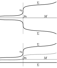
Figure 2. In the top figure, $\Sigma$ is a smooth hypersurface of $TM\equiv\mathds{R}^{2}$ consisting of two curves which intersect the vertical space at $(p_{0},v_{0})$ (depicted as a vertical line) non-transversely. So $\Sigma$ satisfies the property (a) in Definition 2.8 and (as the curves are symmetric with respect to the zero section of $TM$) it determines continuously a scalar product in the tangent space at each $p\in M\equiv\mathds{R}$. Nevertheless, the failure of (b) implies that this product does not vary smoothly with respect to $p$ and, so, $\Sigma$ does not determine a (smooth) Riemannian metric on $M$. In the second figure, changing the lower curve by a horizontal line, one obtains at each tangent space a wind Minkowskian structure varying continuously (but not smoothly) with the point. Moreover, the vector field determined by the centroids (the dashed curve) is not differentiable at $p_{0}$.

Definition 2.17.

Let $\Sigma$ be a wind Finslerian structure on $M$. Then,

$$\tilde{\Sigma}:=-\Sigma:=\{v\in TM:-v\in\Sigma\}$$

is the reverse wind Finslerian structure of $\Sigma$.

Obviously, $\tilde{\Sigma}$ is a wind Finslerian structure too and, from the definition, one gets easily the following.

Proposition 2.18.

Given a wind Finslerian structure $\Sigma$, the conic Finsler metric $\tilde{F}$ and the Lorentzian Finsler one $\tilde{F}_{l}$ associated with the reverse wind Finslerian structure $-\Sigma$ are the (natural) reverse conic pseudo-Finsler metrics of $F$ and $F_{l}$, that is, the domains of $\tilde{F}$ and $\tilde{F}_{l}$ are, respectively, $\tilde{A}=-A=\{v\in TM:-v\in A\}$ and $\tilde{A}_{l}=-A_{l}=\{v\in TM:-v\in A_{l}\}$ and they are defined as $\tilde{F}(v)=F(-v)$ for every $v\in\tilde{A}$ and $\tilde{F}_{l}(v)=F_{l}(-v)$ for every $v\in\tilde{A}_{l}$.

2.3. Wind lengths and balls

In order to deal with curves, the following conventions will be useful.

Convention 2.19.

For any wind Finslerian structure $\Sigma$ we extend $F$ and $F_{l}$ to $A\cup A_{E}$ as follows. First, consistently with Proposition 2.12, $F$ and $F_{l}$ are regarded as continuously extended to the boundary of $A_{l}$ in $TM_{l}\setminus\mathbf{0}$. $F_{l}$ is extended as equal to $+\infty$ on $A$ in the regions of mild and critical wind i.e. on the set $\{v\in A_{p}:0_{p}\in\bar{B}_{p}\}$ (that is, $F_{l}$ is equal to $+\infty$ on the vectors where $F$ has been defined and $F_{l}$ has not). Finally, we define $F_{l}$ and $F$ as equal to $1$ on the set of critical wind zeroes (i.e., the set $\{0_{p}:0_{p}\in\Sigma_{p}\}$, which was included in the definition of $A_{E}$, Definition 2.11). Notice that neither this choice of $F_{l}$ and $F$ on the critical wind region nor any other can ensure their continuity; however, $F_{l}$ and $F$ are continuous on $A\cup(A_{E}\setminus\mathbf{0})$. We also use natural notation such as $(A_{l})_{p}=A_{l}\cap T_{p}M$, $(A_{E})_{p}=A_{E}\cap T_{p}M$.

To understand this choice, recall first that the necessity to extend $A$ to $A_{E}$ in the critical and strong wind regions comes from the fact that all the indicatrices $\Sigma_{p}$ should be contained in $A_{E}$. In the critical region, $\Sigma_{p}\setminus\{0_{p}\}$ lies in $A$ and, so, in the domain of $F$. Therefore, it is not strange to include $0_{p}$ in $A_{E}$ so that $F_{l}$ is defined on this vector and, obviously, the choice $F_{l}(0_{p})=F(0_{p})=1$ comes from the fact that $0_{p}$ lies in the indicatrix and in the boundary of $A_{E}$. A further support for these choices will come from the viewpoint of spacetimes, as the vectors in $A\cup A_{E}$ are those which can be obtained as the projection of a lightlike vector in the spacetime.

As usual, a piecewise smooth curve $\gamma$ will be defined in a compact interval $I=[a,b]$, and it will be smooth except in a finite number of breaks $t_{i}\in I$, $i\in\{1,\dots,k\}$, where it is continuous and its one-sided derivatives are well defined; its reparametrizations will be assumed also piecewise smooth and with positive one-sided derivatives (so that, for example a piecewise smooth geodesic with proportional one-sided derivatives at each break pointing in the same direction can be reparametrized as smooth geodesics), unless otherwise specified.

Definition 2.20.

Let $\Sigma$ be a wind Finslerian structure with associated pseudo-Finsler metrics $F$ and $F_{l}$ and consider a piecewise smooth curve $\gamma:[a,b]\subset\mathds{R}\rightarrow M$, $a<b$.

(i) $\gamma$ is $\Sigma$-admissible if its left and right derivatives $\dot{\gamma}(s^{-}),\dot{\gamma}(s^{+})$ belong to $A\cup A_{E}$ at every $s\in[a,b]$. Analogously, $\gamma$ is $F$-admissible if $\dot{\gamma}(s^{\pm})\in A$, for each $s\in[a,b]$. Accordingly, a vector field $V$ on $M$ is $\Sigma$-admissible (resp. $F$-admissible) if $V_{p}\in A\cup A_{E}$ for each $p\in M$, (resp. $V_{p}\in A$ for each $p\in M$).

(ii) A $\Sigma$-admissible curve $\gamma$ is a wind curve if

$$F(\dot{\gamma}(s))\leq 1\leq F_{l}(\dot{\gamma}(s))\quad\quad\forall s\in[a,b],$$ (6)

and an $F$-admissible wind curve will be called just $F$-wind curve.

(iii) A $\Sigma$-admissible curve $\gamma$ is a regular curve if its one-sided derivatives can vanish only at isolated points (which can be regarded as break points, even though the curve may be smooth there), and it is a strictly regular curve if its one-sided derivatives (and, thus, its velocity outside the breaks) cannot vanish at any point.

(iv) The wind lengths of a $\Sigma$-admissible curve $\gamma$ (not necessarily a wind curve) are defined as

$$\ell_{F}(\gamma) =\int_{a}^{b}F(\dot{\gamma})ds\ \big{(}\!\!\in(0,+\infty]\big{)}, \ell_{F_{l}}(\gamma) =\int_{a}^{b}F_{l}(\dot{\gamma})ds\ \big{(}\!\!\in(0,+\infty]\big{)}.$$

Obviously, from (6) we get:

Proposition 2.21.

If $\gamma$ is a wind curve then

$$\ell_{F}(\gamma|_{[a^{\prime},b^{\prime}]})\leq b^{\prime}-a^{\prime}\leq\ell_{F_{l}}(\gamma|_{[a^{\prime},b^{\prime}]}),\quad\text{for all $a\leq a^{\prime}<b^{\prime}\leq b$.}$$ (7)

We will use this and other natural properties (as the fact that the concatenation of two wind curves $\gamma_{1},\gamma_{2}$ such that $\gamma_{1}(b_{1})=\gamma_{2}(a_{2})$ is another wind curve) with no further mention.

Remark 2.22.

Wind curves collect the intuitive idea of Zermelo’s navigation problem, namely: the possible velocities attained by the moving object are those satisfying the inequalities in (6) (observe that in the region $M\setminus M_{l}$, the inequalities in (6) reduce to $F(\dot{\gamma}(s))\leq 1$). These velocities never include $0_{p}$ if $p\in M_{l}$ and must include $0_{p}$ if $0_{p}\in\overline{B}_{p}$, which happens iff $p\in M\setminus M_{l}$, even though, by convenience, we have excluded $0_{p}$ from $A_{p}$ if $p\in M_{mild}$ and included it in the extended domain $A_{E}$ when $p\in M_{crit}$. The reason to exclude $0_{p}$ from $A_{p}$ when $p\in M_{mild}$ is just to emphasize the different role of the zero vector in this region and in $M_{crit}$ (as well as avoiding problems of differentiability with $F$). In fact, in order to connect points by means of curves included in $M_{mild}$, one can avoid to use velocities that vanish (and this may be convenient for purposes such as reparametrizing the curve at constant speed; such an assumption is frequent in Riemannian Geometry too). However, as in the case of Riemannian Geometry, the vanishing of the velocity in subsets with accumulation points leads to bothering problems about its reparametrizations. So, we will consider the solutions of Zermelo’s problem as regular wind curves (allowing the velocity to vanish in isolated points), and we will ensure the existence of such solutions (see Corollary 6.18). Observe also that the continuity of $F\circ\dot{\gamma}$ and $F_{l}\circ\dot{\gamma}$ has to be checked only when $\dot{\gamma}(s)$ is equal to a zero of the critical region (see Proposition 2.30-(ii)) and, in this case, $F$ and $F_{l}$ are defined as equal to $1$ there. A further explanation of this choice is provided in Example 2.23 below, where two paradigmatic examples of curves with Kropina’s zeroes in the derivatives are given.

Example 2.23.

Let $\mathds{R}^{2}$ be endowed with the Kropina norm $F(x,y)=(x^{2}+y^{2})/x$ defined in $A=\{(x,y)\in\mathds{R}^{2}:x>0\}$. Then the curve $\alpha:[0,1]\rightarrow\mathds{R}^{2}$, $\alpha(t)=(t^{2},t^{3})$, satisfies that $\dot{\alpha}(0)=(0,0)$ and $\lim_{t\rightarrow 0}F(\dot{\alpha}(t))=0$. Clearly, the reparametrization of this curve as an $F$-unit curve is not differentiable at $t=0$. In fact, this kind of curves was excluded in the mild region. However, consider the indicatrix of $F$ as a curve, take the part which is $\Sigma$-admissible and reparametrize it as an $F$-unit curve. In such a way, we get a curve $\gamma:[a,b]\rightarrow\mathds{R}^{2}$ whose derivative is zero in the two end-points, but with $F\circ\dot{\gamma}$ constantly equal to $1$. This second kind of curves is the main reason for including the zero in the Kropina region in the domains of $F$ and $F_{l}$. Observe that if one wants to exclude the first kind of curves, it is enough to require the continuity of $F\circ\dot{\gamma}$ in the definition of wind curves in every smooth piece.

Let $x_{0},x_{1}\in M$ and let us denote by $C^{\Sigma}_{x_{0},x_{1}}$ (resp. $C^{A}_{x_{0},x_{1}}$, $\Omega^{A}_{x_{0},x_{1}}$) the set of the wind curves (resp. $F$-wind curves, $F$-admissible curves) between $x_{0}$ and $x_{1}$ (each curve $\gamma$ defined in a possibly different interval $[a_{\gamma},b_{\gamma}]$).

Following [51], we introduce the following notions.

Definition 2.24.

Given a conic pseudo-Finsler metric $F\colon A\subset TM\to[0,+\infty)$, the Finslerian separation, also called $F$-separation, $d_{F}\colon M\times M\to[0,+\infty]$ is defined as $d_{F}(p,q)=\inf_{\gamma\in\Omega^{A}_{x_{0},x_{1}}}\ell_{F}(\gamma)$ if $\Omega^{A}_{x_{0},x_{1}}\neq\emptyset$ otherwise $d_{F}(p,q)=+\infty$. By using the Finslerian separation two families of subsets of $M$ can be introduced: for any $x_{0}\in M$ and $r\in(0,+\infty)$, set $B_{F}^{+}(x_{0},r)=\{y\in M:d_{F}(x_{0},y)<r\}$ and $B^{-}_{F}(x_{0},r)=\{y\in M:d_{F}(y,x_{0})<r\}$. Moreover, a conic pseudo-Finsler metric is said Riemannianly lower bounded on an open subset $D$ of $M$ if there exists a Riemannian metric $g_{0}$ on $M$ such that $F(v)\geq\sqrt{g_{0}(v,v)}$, for all $v\in TD\cap A$.

As $F$ and $F_{l}$ are continuously extendible to $A_{E}\setminus\mathbf{0}$, we immediately get, by homogeneity, that they are Riemannianly lower bounded on, respectively, $M$ and $M_{l}$. By [51, Proposition 3.13], the collections $B_{F}^{\pm}(x_{0},r)$ of a Riemannianly lower bounded conic pseudo-Finsler $F$ constitute a basis for the topology of $D$, thus we have:

Proposition 2.25.

The collections of $B_{F}^{\pm}(x_{0},r)$ (resp $B_{F_{l}}^{\pm}(x_{0},r)$) constitute a basis for the topology of $M$ (resp. $M_{l}$).

Some cautions, however, must be taken. For example, the Finslerian separation of the conic Finsler metric $F$ may be discontinuous; in fact, the conic Finsler metric in [51, Example 3.18] exhibits this property (see also Section 4 below). We refer to [51, Section 3.5] for a summary of the properties satisfied by the Fnslerian separation.

In order to work with the full geometry associated with $\Sigma$ we also introduce the following new collections of subsets of $M$.

Definition 2.26.

Let $x_{0}\in M$ and $r>0$. The forward (resp. backward) wind balls of center $x_{0}$ and radius $r$ associated with the wind Finslerian structure $\Sigma$ are:

$$B^{+}_{\Sigma}(x_{0},r)=\{x\in M:\ \exists\ \gamma\in C^{\Sigma}_{x_{0},x},\text{ s.t. }r=b_{\gamma}-a_{\gamma}\,\text{and}\;\ell_{F}(\gamma)<r<\ell_{F_{l}}(\gamma)\},$$

$$B^{-}_{\Sigma}(x_{0},r)=\{x\in M:\ \exists\ \gamma\in C^{\Sigma}_{x,x_{0}},\text{ s.t. }r=b_{\gamma}-a_{\gamma}\,\text{and}\;\ell_{F}(\gamma)<r<\ell_{F_{l}}(\gamma)\}.$$

being the closed balls $$\bar{B}^{\pm}_{\Sigma}(x_{0},r)$$ their closures. Moreover, the (forward, backward) c-balls are defined as:

$$\hat{B}^{+}_{\Sigma}(x_{0},r)=\{x\in M:\ \exists\ \gamma\in C^{\Sigma}_{x_{0},x},\text{ s.t. }r=b_{\gamma}-a_{\gamma}\,\text{(so,}\;\ell_{F}(\gamma)\leq r\leq\ell_{F_{l}}(\gamma))\},$$

$$\hat{B}^{-}_{\Sigma}(x_{0},r)=\{x\in M:\ \exists\ \gamma\in C^{\Sigma}_{x,x_{0}},\text{ s.t. }r=b_{\gamma}-a_{\gamma}\,\text{(so,}\;\ell_{F}(\gamma)\leq r\leq\ell_{F_{l}}(\gamma))\}$$

for $r>0$ and, by convention for $r=0$, $\hat{B}^{\pm}_{\Sigma}(x_{0},0)=x_{0}$.

Recall that, consistently with our conventions, if $0_{x_{0}}\in\Sigma_{x_{0}}$ then $x_{0}\in\hat{B}^{\pm}_{\Sigma}(x_{0},r)$ for all $r\geq 0$ (this will be interpreted naturally in the description of the causal future of a point in an $\rm SSTK$ see, e.g. Proposition 5.1).

Proposition 2.27.

If a wind Finslerian structure comes from a Finsler one then the sets $B^{+}_{\Sigma}(x_{0},r)$ and $B^{-}_{\Sigma}(x_{0},r)$, $r>0$, coincide with the standard forward and backward open balls centred at $x_{0}$.

Proof.

Just take into account that the assumption is equivalent to $0\in B_{p}$, for all $p\in M$ and, according to Convention 2.19, $F_{l}(v)=+\infty$, for all $v\in A=TM\setminus\mathbf{0}$. ∎

Example 2.28.

$\hat{B}^{+}_{\Sigma}(x_{0},r)$ and $\hat{B}^{-}_{\Sigma}(x_{0},r)$ do not coincide in general with the closures $\bar{B}_{\Sigma}^{+}(x_{0},r)$ and $\bar{B}_{\Sigma}^{-}(x_{0},r)$. This may occur even when $\Sigma$ comes from a Riemannian metric (in $\mathds{R}^{2}\setminus\{(1,0)\}$, $\hat{B}^{+}_{\Sigma}(0,2)$ is not closed); another simple example (using a strong wind Minkowskian structure) can be seen in Fig. 3. In fact, as we will see, the closedness of the c-balls will be related with the convexity of the manifold.

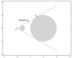
Figure 3. A wind Minkowskian structure $\Sigma$ in $\mathds{R}^{2}\setminus\{Q\}$. The shaded regions represent the wind balls $B^{+}_{\Sigma}(0,1/5)$ and $B^{+}_{\Sigma}(0,1)$ which satisfy $\hat{B}^{+}_{\Sigma}(0,1/5)=\bar{B}^{+}_{\Sigma}(0,1/5)$ but $P\in\bar{B}^{+}_{\Sigma}(0,1)\setminus\hat{B}^{+}_{\Sigma}(0,1)$.

The next three propositions provide a better understanding of $\hat{B}^{\pm}_{\Sigma}(x_{0},r)$. Before them, we will prove a technical lemma, which stresses the importance of transversality (recall Example 2.16).

Lemma 2.29.

Let $\Sigma$ be a wind Finslerian structure on $M$ and $p\in M$ such that $0_{p}\in\Sigma_{p}$, and let $\gamma:(-\varepsilon,\varepsilon)\rightarrow M$ be a smooth $F$-admissible curve such that $\gamma(0)=p$. Then, reducing $\varepsilon$ if necessary, the surface

$$T_{\gamma}=\{\lambda\dot{\gamma}(s):\lambda\in\mathds{R},s\in(-\varepsilon,\varepsilon)\}$$

is embedded in $TM$ and it is transverse to $\Sigma$. Moreover, if $\varepsilon$ is small enough, a smooth function $(-\varepsilon,\varepsilon)\ni s\mapsto\lambda(s)\in\mathds{R}$ is obtained by requiring that each $\lambda(s)\dot{\gamma}(s)$ be the point in $\Sigma_{\gamma(s)}\cap T_{\gamma}=\{\lambda_{1}\dot{\gamma}(s),\lambda_{2}\dot{\gamma}(s)\}$ with smaller $|\lambda_{i}|,i=1,2$.

Proof.

Clearly, $T_{\gamma}$ is embedded and it cuts $\Sigma$ transversely in two points because $\dot{\gamma}(s)\in A$ for every $s\in(-\varepsilon,\varepsilon)$ (with $\varepsilon>0$ small enough). So, $T_{\gamma}$ fulfils the required property of transversality and, moreover, $\Sigma\cap T_{\gamma}$ is composed by two connected one-dimensional smooth submanifolds $\rho_{1}$, which contains $0_{p}$, and $\rho_{2}$. The parameter $s$ of $\gamma$ can be chosen as a natural coordinate for $\rho_{1}$. In this coordinate, the inclusion of $\rho_{1}$ in $TM$ is the smooth map $s\mapsto\lambda(s)\dot{\gamma}(s)$, so that the map $\lambda$ is smooth. ∎

Proposition 2.30.

With the above notation:

1. Let $(M,\Sigma)$, $p\in M$, $0_{p}\in\Sigma_{p}$ and $\gamma:(-\varepsilon,\varepsilon)\rightarrow M$, $\gamma(0)=p$, smooth and $F$-admissible, as in the previous lemma. Then, $\ell_{F_{l}}(\gamma|_{[0,\varepsilon^{\prime}]})=+\infty$ for all $0<\varepsilon^{\prime}\leq\varepsilon$. As a consequence, for each $r_{0}>0$ there exists $\varepsilon_{0}\leq\varepsilon$ such that $\gamma((0,\varepsilon_{0}])\subset B^{+}_{\Sigma}(p,r)$ for all $r\geq r_{0}$.

2. If a smooth curve $\gamma\colon[a,b]\to M$ is $\Sigma$-admissible and strictly regular, then $F\circ\dot{\gamma}$ and $F_{l}\circ\dot{\gamma}$ are continuous (the latter as a map from $[a,b]$ to $(0,+\infty]$).

3. A $\Sigma$-admissible curve $\gamma:[a,b]\rightarrow M$ satisfies $\ell_{F_{l}}(\gamma)=+\infty$ if $F_{l}(\dot{\gamma}(s_{0}))=+\infty$ at some $s_{0}\in[a,b]$. The converse holds when $\gamma$ is strictly regular.

4. For any $\Sigma$-admissible curve,

   $$\ell_{F}(\gamma)\leq\ell_{F_{l}}(\gamma)$$ (8)

   with equality iff $\dot{\gamma}(s)\in A_{E}\setminus A$. Moreover, for a wind curve satisfying the equality in (8), $F_{l}(\dot{\gamma})=F(\dot{\gamma})\equiv 1$ everywhere.

Proof.

$(i)$ Choose any sequence $\varepsilon_{k}\searrow 0$ in $(0,\varepsilon)$. Clearly, we have $\gamma(\varepsilon_{k})\rightarrow p$ and $\ell_{F}(\gamma|_{[0,\varepsilon_{k}]})\searrow 0$; so, it is enough to prove that $\ell_{F_{l}}(\gamma|_{[0,\varepsilon_{k}]})=+\infty$ for all $k$. From the definition of $\lambda(s)$ in Lemma 2.29 and $F_{l}$, we have

$$F_{l}(\dot{\gamma}(s))=\left\{\begin{array}[]{lcrl}1/\lambda(s)&&\hbox{if}&\lambda(s)>0\\ +\infty&&\hbox{if}&\lambda(s)\leq 0\\ \end{array}\right.$$ (9)

As $\lambda(0)=0$ and $\lambda$ is smooth around $0$

$$\int_{0}^{\varepsilon_{k}}\frac{ds}{\lambda(s)}=+\infty,$$

and all the assertions follow directly.

$(ii)$ Observe that $F\circ\dot{\gamma}$ is always continuous in this case and $F_{l}\circ\dot{\gamma}$ can be discontinuous in $s_{0}\in[a,b]$, only when $\gamma(s_{0})$ belongs to $M_{crit}$. Moreover, in this case, $\gamma$ has to be $F$-admissible in a neighborhood of $s_{0}$ because it is smooth and strictly regular. Then applying Lemma 2.29 in order to get (9) to the reparametrization $\tilde{\gamma}(s)=\gamma(s-s_{0})$, we conclude.

$(iii)$ Necessarily, $\gamma(s_{0})$ must belong either to $M_{crit}$, and the part $(i)$ applies (recall that, being $F_{l}(\dot{\gamma}(s_{0}))=+\infty$, $\dot{\gamma}(s_{0})\in A_{\gamma(s_{0})}$ and $\gamma$ must be $F$-admissible and smooth in a right or a left neighborhood of $s_{0}$), or to $M_{mild}$ and $F_{l}(\dot{\gamma})=+\infty$ in some neighborhood of $s_{0}$. For the converse, notice that at least one of the smooth pieces of $\gamma$ has to be of infinite $F_{l}$-length then, necessarily, $F_{l}(\dot{\gamma}(s_{0}))=+\infty$ for at least one point $s_{0}\in[a,b]$ otherwise the $F_{l}$-length of such a piece would be finite by part $(ii)$.

$(iv)$ Apply Proposition 2.12 and Convention 2.19. ∎

Remark 2.31.

$F$-admissible curves are always strictly regular $\Sigma$-admissible ones. For these curves, $\ell_{F_{l}}(\gamma)$ may be infinite even in the case of an $F$-admissible curve contained in $M_{l}$ except at one endpoint, see Proposition 2.30. The role of strict regularity becomes apparent from the discussion in Convention 2.19 (see also Proposition 2.32 below).

Notice that wind curves depend on reparametrizations. However, the following result suggests that this is not a relevant restriction, at least when the velocities do not vanish; it also provides a control on the possible reparametrizations.

Proposition 2.32.

Let $\gamma$ be a piecewise smooth $\Sigma$-admissible curve such that, in each interval where $\gamma$ is smooth, $F\circ\dot{\gamma}$ is continuous and $F_{l}\circ\dot{\gamma}$ is either infinite at some point or continuous. Then, $\gamma$ admits a (piecewise smooth) reparametrization $\tilde{\gamma}:[0,r_{0}]\rightarrow M$ as a wind curve and, necessarily then, $\ell_{F}(\gamma)\leq r_{0}\leq\ell_{F_{l}}(\gamma)$. Moreover, $r_{0}$ can be chosen equal to any value of $[\ell_{F}(\gamma),\ell_{F_{l}}(\gamma)]$ if $\ell_{F_{l}}(\gamma)<+\infty$, and, any value of $[\ell_{F}(\gamma),+\infty)$ otherwise. In particular, this applies for any strictly regular $\Sigma$-admissible curve and, therefore, for any $F$-admissible curve.

Proof.

We can assume that $\gamma$ is smooth because the piecewise smooth case trivially follows from this. Put $\tilde{\gamma}(r)=\gamma(s(r))$. The reparametrization $s(r)$ as a wind curve is characterized by

$$F(\dot{\gamma}(s(r)))\dot{s}(r)\leq 1\leq F_{l}(\dot{\gamma}(s(r)))\dot{s}(r).$$

As $F\circ\dot{\gamma}$ is continuous, we can first reparametrize $\gamma$ with $F(\dot{\gamma})\equiv 1$. Clearly, this gives also a parametrization of $\gamma$ as a wind curve. In order to prove the last part of the proposition let us distinguish three cases:

(a) If $F_{l}(\dot{\gamma})<+\infty$ at all the points then, by assumptions, $F_{l}\circ\dot{\gamma}$ is continuous and the family of reparametrizations, defined by $\dot{r}_{\lambda}(s)=\lambda F_{l}(\dot{\gamma}(s))+(1-\lambda)F(\dot{\gamma}(s)),\lambda\in[0,1]$, is enough to obtain all the required values of $r_{0}$.

(b) If $F_{l}(\dot{\gamma}(\bar{s}))=+\infty$, for some $\bar{s}\in[a,b]$, and $F_{l}\circ\dot{\gamma}$ is continuous (as a map assuming values in $(0,+\infty]$) everywhere, then, by Proposition 2.30-(iii), $\ell_{F_{l}}(\gamma)=+\infty$ and the conclusion follows modifying the expression of $\dot{r}_{\lambda}$ in case (a) by substituting $F_{l}(\dot{\gamma}(s))$ with $\varphi_{\lambda}(F_{l}(\dot{\gamma}(s)))$, $\lambda\in[0,1)]$, where:

$$\varphi_{\lambda}(t)=\left\{\begin{array}[]{ll}t&\hbox{if}\;t\leq 1/(1-\lambda)\\ \phi_{0}(t-1/(1-\lambda))+1/(1-\lambda)&\hbox{if}\;t\in\left(1/(1-\lambda),2+1/(1-\lambda)\right)\\ 1+1/(1-\lambda)&\hbox{if}\;t\geq 2+1/(1-\lambda)\end{array}\right.$$

being $\phi_{0}:[0,2]\rightarrow[0,1]$ any curve with $\phi_{0}(t)\leq t,t\in[0,2]$ that connects smoothly the graphs of $t\mapsto t$ for $t\leq 0$ and of $t\mapsto 1$ for $t\geq 2$, and recalling that we have assumed $F(\dot{\gamma})=1$.

(c) Finally, if $F_{l}(\dot{\gamma}(\bar{s}))=+\infty$, for some $\bar{s}\in[a,b]$, then $\gamma$ must be strictly regular in a neighbourhood $[a^{\prime},b^{\prime}]$ of $\bar{s}$ and then, by Proposition 2.30-(ii), $F_{l}\circ\dot{\gamma}$ must be continuous in $[a^{\prime},b^{\prime}]$. Therefore, as in case (b), we can change the parametrization of $\gamma$ only on the interval $[a^{\prime},b^{\prime}]$ to get all the values $r_{0}\in[\ell_{F}(\gamma),+\infty)$ also in this case.

∎

Proposition 2.33.

For any wind Finslerian structure $\Sigma$ and $r>0$:

$$B^{+}_{\Sigma}(x_{0},r)\subset\hat{B}^{+}_{\Sigma}(x_{0},r)\subset\bar{B}_{\Sigma}^{+}(x_{0},r),$$

$$B^{-}_{\Sigma}(x_{0},r)\subset\hat{B}^{-}_{\Sigma}(x_{0},r)\subset\bar{B}_{\Sigma}^{-}(x_{0},r).$$

Thus, the closures of ${B}_{\Sigma}^{+}(x,r)$ and $\hat{B}_{\Sigma}^{+}(x,r)$ are equal.

Proof.

The first inclusions follow trivially from the definitions. Let $x\in\hat{B}^{+}_{\Sigma}(x_{0},r)$ and consider a wind curve $\gamma\colon[a,b]\to M$ from $x_{0}$ to $x$ such that $\ell_{F}(\gamma)\leq r=b-a\leq\ell_{F_{l}}(\gamma)$. If the two inequalities held strictly, there would be nothing to prove. Otherwise, consider the following cases:

(a) $\ell_{F}(\gamma)=r=\ell_{F_{l}}(\gamma)$ (in particular, $\dot{\gamma}(s)\in A_{E}\setminus A$ for all $s$ and $F(\dot{\gamma})\equiv 1$, recall Remark 2.31(2)). Choose any $F$-admissible vector field $V$ such that $F(V)\equiv 1$ defined in some neighborhood $U$ of $x$; notice that the integral curves of $V$ are wind curves. Take a smaller neighborhood $U^{\prime}$ and some $\varepsilon>0$ so that the flow of $V$ is defined in $[0,\varepsilon]\times U^{\prime}$ and $\gamma([b-\varepsilon,b])\subset U^{\prime}$. Choose $\{s_{n}\}\nearrow b$ and consider the curve $\gamma_{n}$ obtained by concatenating $\gamma|_{[a,s_{n}]}$ and the integral curve $\rho_{n}:[0,\varepsilon_{n}]\rightarrow M$ of $V$ starting at $\gamma(s_{n})$, where $\varepsilon_{n}:=b-s_{n}>0$. By construction, $\ell_{F}(\rho_{n})=\varepsilon_{n}=\ell_{F}(\gamma|_{[b-s_{n},b]})$ and $\ell_{F}(\gamma_{n})=r<\ell_{F_{l}}(\gamma_{n})$. So, choosing some close $\varepsilon^{\prime}_{n}<\varepsilon_{n}$, the lengths of the corresponding restriction of $\gamma_{n}$ allow us to write $\rho_{n}(\varepsilon^{\prime}_{n})\in B^{+}_{\Sigma}(x_{0},r)$ and $\rho_{n}(\varepsilon^{\prime}_{n})\to x$, as required.

(b) $\ell_{F}(\gamma)=r<\ell_{F_{l}}(\gamma)$. Just notice that the points $\gamma(b-\varepsilon)$ will belong to $B^{+}_{\Sigma}(x_{0},r)$ for small $\varepsilon$.

(c) $\ell_{F}(\gamma)<r\leq\ell_{F_{l}}(\gamma)$. Extending $\gamma$ beyond $b$ by concatenating an $F$-admissible piece, the points in the extension close to $x$ will belong to $B^{+}_{\Sigma}(x_{0},r)$.

∎

Finally, an interpretation of the c-balls is provided for the classical Finsler case. Notice that, in this case, the restriction for a piecewise smooth curve to be “wind” is just to assume that its speed is not bigger than 1 (in order to travel not faster than the maximum allowed speed) and the velocity not to be 0 (by convenience, see Remark 2.22 (3)); so, there are no relevant restrictions from a practical viewpoint.

Proposition 2.34.

Let $(M,F)$ be a connected Finsler manifold and $\Sigma$ its indicatrix, regarded as a wind Finslerian structure with forward and backward balls $B^{+}_{F}(x_{0},r)(=B^{+}_{\Sigma}(x_{0},r))$ and $B^{-}_{F}(x_{0},r)(=B^{-}_{\Sigma}(x_{0},r))$. The following assertions are equivalent:

1. $\hat{B}^{+}_{\Sigma}(x_{0},r)=\bar{B}^{+}_{F}(x_{0},r)$ for all $x_{0}\in M,r>0$.

2. $\hat{B}^{-}_{\Sigma}(x_{0},r)=\bar{B}^{-}_{F}(x_{0},r)$ for all $x_{0}\in M,r>0$.

3. $(M,F)$ is (geodesically) convex, i.e., any pair of points $(p,q)$ can be connected by a geodesic of length equal to the Finsler distance $d_{F}(p,q)$.

Proof.

We will consider only the equivalence between $(i)$ and $(iii)$, as the convexity of $F$ is equivalent to the convexity of its reverse metric $\tilde{F}$.

$(iii)\Rightarrow(i)$. Otherwise, there exists some $x_{1}\in\bar{B}^{+}_{F}(x_{0},r)\setminus\hat{B}^{+}_{\Sigma}(x_{0},r)$ and, by the continuity of the distance, $d_{F}(x_{0},x_{1})=r$. But no curve of length equal to $r$ can join these points, which contradicts geodesic convexity.

$(i)\Rightarrow(iii)$. Straightforward from the definitions (recall that when the wind Finslerian structure is Finsler, $F_{l}=+\infty$ and a minimizing curve must be a geodesic). ∎

2.4. Geodesics

We aim now to introduce a notion of geodesic for a wind Finslerian structure which recovers the standard one for $F$ and $F_{l}$. As the radius corresponding to each $v\in\Sigma\cap(A_{E}\setminus A)$ is not transversal to $\Sigma$, $\Sigma$ does not carry a globally defined smooth contact form such that the flow of its associated Reeb vector field is compatible with the geodesic flow of both $F$ and $F_{l}$ (compare with [15, Section 2]). Thus, we start by defining extremizing geodesics of $\Sigma$ by unifying local extremizing properties of both type of geodesics as follows.

Definition 2.35.

Let $(M,\Sigma)$ be a wind Finslerian manifold. A wind curve $\gamma:[a,b]\to M$, $a<b$, is called a unit extremizing geodesic if

$$\gamma(b)\in\hat{B}_{\Sigma}^{+}(\gamma(a),b-a)\setminus B_{\Sigma}^{+}(\gamma(a),b-a).$$ (10)

We will say that $\gamma$ is an extremizing geodesic (resp. pregeodesic) if it is an affine (resp. arbitrary, according to the end of Convention 2.19) reparametrization of a unit extremizing geodesic.

Some elementary properties of these geodesics are the following.

Proposition 2.36.

Let $(M,\Sigma)$ be a wind Finsler structure.

1. If $\gamma$ is a unit extremizing geodesic of $(M,\Sigma)$, then:

   1. its restriction $\gamma_{|[a^{\prime},b^{\prime}]}$ to any subinterval $[a^{\prime},b^{\prime}],a\leq a^{\prime}<b^{\prime}\leq b$ is also a unit extremizing geodesic. In particular,

      $$\gamma(t)\in\hat{B}_{\Sigma}^{+}(\gamma(a),t-a)\setminus B_{\Sigma}^{+}(\gamma(a),t-a)$$

      for every $t\in[a,b]$;

   2. at least one of the following two properties holds:

      $$\gamma(b)\notin B^{+}_{\Sigma}(\gamma(a),\ell_{F}(\gamma)),$$ (11)

      $$\gamma(b)\notin B^{+}_{\Sigma}(\gamma(a),\ell_{F_{l}}(\gamma))\quad\quad(\hbox{with }\quad\ell_{F_{l}}(\gamma)<+\infty).$$ (12)

      Moreover, in the first case, $F(\dot{\gamma})\equiv 1$ everywhere and in the second one $F_{l}(\dot{\gamma})\equiv 1$ everywhere.

2. If a wind curve $\gamma$ satisfies (11) (resp. (12)), then this same property holds for the restriction $\gamma_{|[a^{\prime},b^{\prime}]}$. Moreover, if $\gamma$ is also strictly regular or, more generally, it satisfies the hypotheses in Proposition 2.32, then it is an extremizing pregeodesic.

3. If a constant curve $\gamma_{x_{0}}(t)=x_{0}$ for all $t\in[a,b]$ is a (unit) extremizing geodesic then $x_{0}\in M_{crit}$. In this case, $\gamma_{x_{0}}$ will be called an extremizing exceptional geodesic.

Proof.

$(i)$ For $(a)$, assume by contradiction that (10) is violated in a subinterval so that $\gamma(b^{\prime})\in B_{\Sigma}^{+}(\gamma(a^{\prime}),b^{\prime}-a^{\prime})$ (recall that (7) holds). So, there will exist a wind curve $\tilde{\gamma}:[a^{\prime},b^{\prime}]\rightarrow M$ satisfying both strict inequalities in (7), and so will do the concatenation $\gamma_{1}\colon[a,b]\to M$ of $\gamma|_{[a,a^{\prime}]},\tilde{\gamma}$ and $\gamma|_{[b,b^{\prime}]}$ defined as

$$\gamma_{1}(t)=\begin{cases}\gamma(t)&\text{if $t\in[a,b]\setminus[a^{\prime},b^{\prime}]$,}\\ \tilde{\gamma}(t)&\text{if $t\in[a^{\prime},b^{\prime}]$,}\end{cases}$$

in contradiction with (10) (for all the interval $[a,b]$).

For $(b)$, notice that by the assumptions,

$$\gamma(b)\not\in B_{\Sigma}^{+}(\gamma(a),b-a)$$ (13)

and $\ell_{F}(\gamma)\leq b-a\leq\ell_{F_{l}}(\gamma)$. Moreover, (13) implies that at least one of the inequalities must be an equality; so, replace $b-a$ with $\ell_{F}(\gamma)$ or $\ell_{F_{l}}(\gamma)$ in (13). For the last assertion, observe that, among the points where $F\circ\dot{\gamma}$ and $F_{l}\circ\dot{\gamma}$ can be different from $1$, they are continuous except in the (finite set of) breaks.

$(ii)$ The curve $\tilde{\gamma}$ which shows that (11) (resp. (12)) does not hold for $\gamma_{|[a^{\prime},b^{\prime}]}$, can be concatenated (as in $(a)$ above) to obtain the contradiction that neither this property could hold for $\gamma$.

For the last assertion, reparametrize $\gamma$ as a wind curve with domain $[0,\ell_{F}(\gamma)]$ or $[0,\ell_{F_{l}}(\gamma)]$, (see Proposition 2.32), and (10) must hold.

$(iii)$ By our conventions, $\gamma_{x_{0}}$ is $\Sigma$- admissible only when $x_{0}\in M_{crit}$. ∎

Proposition  2.36 $(i)$-$(b)$ suggests that extremizing pregeodesics satisfy minimization or maximization properties. Let us introduce a natural variational setting.

Definition 2.37.

Let $\gamma\colon[a,b]\to M$ be a wind curve between $x_{0}$ and $x_{1}$, and assume that $\{a=t_{0}\leq\ldots\leq t_{n}=b\}$ is a subset of the interval $[a,b]$ such that $\gamma_{|[t_{i-1},t_{i}]}$ is smooth, for each $i\in\{1,\ldots,n\}$. Let $C^{\Sigma}_{x_{0},x_{1}}[a,b]:=\{\rho\in C^{\Sigma}_{x_{0},x_{1}}:\text{ $\rho$ is defined on $[a,b]$}\}$, and analogously let $C^{A}_{x_{0},x_{1}}[a,b]=\{\rho\in C^{A}_{x_{0},x_{1}}:\text{ $\rho$ is defined }$ $\text{on $[a,b]$}\}$. A (proper) wind variation of $\gamma$ is a continuous map $\psi\colon(-\varepsilon,\varepsilon)\times[a,b]\to M$, such that $\psi=\psi(s,t)$ is a $C^{2}$ map on $(-\varepsilon,\varepsilon)\times[t_{i-1},t_{i}]$, $\psi(0,\cdot)=\gamma$ and for each $s\in(-\varepsilon,\varepsilon)$, $\psi_{s}\colon=\psi(s,\cdot)\in C^{\Sigma}_{x_{0},x_{1}}[a,b]$. A wind variation will be said an $F$-wind variation if $\psi_{s}\in C^{A}_{x_{0},x_{1}}[a,b]$, for each $s\in(-\varepsilon,\varepsilon)\setminus\{0\}$.

Observe that, according to Definition 2.37, any wind variation of an $F$-wind curve must be $F$-wind (reducing $\varepsilon$ if necessary).

Example 2.38.

The wind restriction for a variation may be somewhat subtle. Consider, for example, the case in that the wind Finsler manifold is just a Riemannian one, and one is looking for wind variations $\psi$ of a unit extremizing geodesic $\gamma:[a,b]\rightarrow M$. Of course, such geodesics are just the minimizing geodesics for the Riemannian manifold parametrized by arc length. For the variation $\psi$ we must impose $F(\dot{\psi}_{s})\leq 1$, and $\ell_{F}(\psi_{s})\leq\ell_{F}(\gamma)$. So, a non-trivial wind variation can exist only when $\gamma(b)$ is the first conjugate point of $\gamma$. The non-existence of such a variation before the first conjugate point means implicitly that $\gamma$ minimizes strictly among nearby curves. Clearly, one can consider also geodesics parametrized at a different speed $c$: in the case $c<1$ wind variations are equal to classical variations but, in the case $c>1$, the geodesic is not a wind curve and, so, no wind variation is defined.

The following result suggests that the question of maximization / minimization becomes somewhat subtle.

Lemma 2.39.

Let $\gamma\in C^{\Sigma}_{x_{0},x_{1}}[a,b]$ be a unit extremizing geodesic satisfying (11), hence $\ell_{F}(\gamma)=b-a\leq\ell_{F_{l}}(\gamma).$ If there exists a wind curve $\alpha\in C^{\Sigma}_{x_{0},x_{1}}[a,b]$ s.t. $\ell_{F}(\alpha)<\ell_{F}(\gamma)$ then $\alpha$ is a unit extremizing geodesic satisfying (12) but not (11), i.e.:

$$\ell_{F}(\alpha)<\ell_{F}(\gamma)=b-a=\ell_{F_{l}}(\alpha)\leq\ell_{F_{l}}(\gamma).$$

Proof.

Being $\alpha$ a wind curve, (7) holds and, so, $b-a=\ell_{F_{l}}(\alpha)$ because, otherwise, $x_{1}\in B_{\Sigma}^{+}(x_{0},b-a)$. ∎

Of course, a dual version of the result holds for the case that $\gamma$ satisfies (12).

Example 2.40.

We emphasize that such an $\alpha$ can exist in some particular cases. In fact, notice first that, for any wind Minkowskian norm $\Sigma$ on $\mathds{R}^{n}$, the unit extremizing geodesics are the straight lines with velocity constantly equal to any vector of $\Sigma$. Now, consider a strong wind Minkowskian example $(\mathds{R}^{2},\Sigma)$ obtained by the displacement of the usual unit sphere by the (constant) vector $(2,0)$, and construct a wind Finslerian cylinder $(S^{1}\times\mathds{R},\Sigma)$ by identifying each $(x,y)$ with $(x+1,y)$, see Fig. 4. Choose the Minkowskian wind c-ball $\hat{B}_{\Sigma}^{+}((0,0),r_{0})\subset\mathds{R}^{2}$ with radius $r_{0}=1/2$. As the natural Euclidean diameter (as a subset of the Euclidean space $\mathds{R}^{2}$) of $\hat{B}_{\Sigma}^{+}((0,0),r_{0})$ is 1, its projection in $S^{1}\times\mathds{R}$ identifies the points $p_{1}=(1/2,0),p_{2}=(3/2,0)$ in a single one $p_{C}$. Then, the univocally determined unit extremizing geodesics $\beta_{1},\beta_{2}:[0,r_{0}]\rightarrow\mathds{R}^{2}$ from $(0,0)$ to $p_{1},p_{2}$ (resp.), project onto geodesics of $S^{1}\times\mathds{R}$ which play the role of $\alpha$ and $\gamma$ in Lemma 2.39.

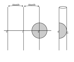
Figure 4. A wind Finslerian cylinder $(S^{1}\times\mathds{R},\Sigma)$. The shaded region represents the c-ball $\hat{B}_{\Sigma}^{+}((0,0),1/2)$

That is, extremizing geodesics are either global minimizers of $\ell_{F}$ or global maximizers of $\ell_{F_{l}}$ on $C^{\Sigma}_{x_{0},x_{1}}[a,b]$ except when a curve $\alpha$ as above appears. However, one can check that such a curve cannot appear among nearby geodesics in the following sense.

Proposition 2.41.

Let $\gamma\colon[a,b]\to M$ be a unit extremizing geodesic between $x_{0}$ and $x_{1}$. Then, one of the following exclusive alternatives holds:

1. $\ell_{F}(\gamma)<\ell_{F_{l}}(\gamma)$ and $x_{1}\not\in B^{+}_{\Sigma}(x_{0},\ell_{F}(\gamma))$ or, equally, $\ell_{F}(\gamma)=b-a<\ell_{F_{l}}(\gamma)$. Then $\gamma$ minimizes the length functional of $F$ between the curves $\psi_{s}$ defined by any wind variation $\psi:(-\epsilon,\epsilon)\times[a,b]\rightarrow M$ of $\gamma$ for $|s|$ sufficiently small ($0\leq|s|<\epsilon^{\prime}$ for some $\epsilon^{\prime}\leq\epsilon$). In this case $\gamma$ will be called a minimizing unit geodesic.

2. $\ell_{F}(\gamma)<\ell_{F_{l}}(\gamma)<+\infty$ and $x_{1}\not\in B^{+}_{\Sigma}(x_{0},\ell_{F_{l}}(\gamma))$ or, equally, $\ell_{F}(\gamma)<b-a=\ell_{F_{l}}(\gamma)$. Then, $\gamma$ maximizes the length functional of $F_{l}$ in a sense analogous to (i) above. In this case, $\gamma$ will be called a maximizing unit geodesic.

3. $\ell_{F}(\gamma)=\ell_{F_{l}}(\gamma)$ (necessarily equal to $b-a$). Then, both (11) and (12) hold, and the velocity of $\gamma$ lies in $A_{E}\setminus A_{l}$. In this case, $\gamma$ will be called a boundary unit geodesic.

Moreover, the restriction of $\gamma$ to any closed subinterval $[a^{\prime},b^{\prime}]$ of $[a,b]$ also satisfies the same type of extremizing property (i), (ii), (iii) as above (minimization, maximization or velocity in $A\setminus A_{l}$ as the original $\gamma$).

Proof.

The distinction of cases comes from Proposition 2.36.

(i) Assume, by contradiction, that there exists a wind variation of $\gamma$ such that for some sequence $s_{n}\to 0$, $\ell_{F}(\psi_{s_{n}})<\ell_{F}(\gamma)$, for each $n\in\mathds{N}$. By Lemma 2.39, $\ell_{F_{l}}(\psi_{s_{n}})=b-a$ and, thus, $F_{l}(\dot{\psi}_{s_{n}})\equiv 1$. As $\{\dot{\psi}_{s_{n}}(t)\}_{n}\rightarrow\dot{\gamma}(t)$ for all $t$, and $F_{l}$ is continuous away from $\mathbf{0}$ (but, there, its value is equal to $1$ too) then $F_{l}(\dot{\gamma})\equiv 1$. As a consequence, a contradiction with the inequality in the lengths of $\gamma$ appears.

(ii) Analogous to part $(i)$.

For (iii) use part (2) of Remark 2.31. For the last assertion, recall the parts $(i)$ and $(ii)$ of Proposition 2.36.

∎

Definition 2.42.

We say that an extremizing geodesic (or more generally, pregeodesic) is minimizing, maximizing or boundary if it can be reparametrized as a unit extremizing geodesic satisfying respectively $(i)$, $(ii)$ or $(iii)$ in Proposition 2.41.

Example 2.43.

Notice that the same geodesic can admit two reparametrizations, one as a minimizing unit geodesic and the other as a maximizing one, so that the possibilities $(i)$ and $(ii)$ are not exclusive. For example, this will happen for all the $\Sigma$- admissible straight lines of a strong wind Minkowskian structure regarded as a wind Finslerian structure. In fact, the straight lines starting at the origin and tangent to the indicatrix determine the boundary geodesics, where both equalities (11) and (12) hold, as the $F$- and $F_{l}$-lengths coincide for each one of them. The straight lines inside this cone also satisfy (11) and (12), even though these lengths are now different, and they consequently admit two different parametrizations as unit geodesics, one with $F(\dot{\gamma})\equiv 1$ (minimizing) and the other one with $F_{l}(\dot{\gamma})\equiv 1$ (maximizing). Notice also that a more classical approach also shows that such lines minimize locally for any conic Finsler norm $F$ (see [51, Section 3.4]), and an analogous reasoning shows that they maximize locally for any Lorentzian norm.

Finally, we arrive at the following definition of geodesic.

Definition 2.44.

Let $I\subset\mathds{R}$ be an interval. We say that a curve $\gamma:I\rightarrow M$ is a unit geodesic of the wind Finslerian structure $(M,\Sigma)$ if, locally, it is a unit extremizing geodesic, namely, for every $t\in I$ there exists $\varepsilon>0$ such that $\gamma|_{[t-\varepsilon,t+\varepsilon]\cap I}$ is a unit extremizing geodesic. We will say that $\gamma$ is a geodesic (resp. pregeodesic) of the wind Finslerian manifold $(M,\Sigma)$ if it is an affine (resp. arbitrary) reparametrization of a unit geodesic. An exceptional geodesic is a constant curve $\gamma_{x_{0}}$ which is locally an extremizing exceptional geodesic (according to Proposition 2.36$(iii)$).

Notice that when the interval $I$ is open, $\epsilon>0$ can be chosen such that $[t-\varepsilon,t+\varepsilon]\subset I$ (in agreement with Definition 2.35), while if $I$ is compact, the intersection with $I$ must be taken properly in the endpoints.

Example 2.43 stresses that a (non-boundary extremizing) geodesic can satisfy simultaneously both (11) and (12) for different “radii”

$$r_{1}(t,\varepsilon)=\ell_{F}(\gamma|_{[t-\varepsilon,t+\varepsilon]\cap I})\text{ and }r_{2}(t,\varepsilon)=\ell_{F_{l}}(\gamma|_{[t-\varepsilon,t+\varepsilon]\cap I}).$$

Thus, the names boundary, and locally minimizing or maximizing can be used only as non-exclusive possibilities.

Proposition 2.34 suggests the following general definition of convexity.

Definition 2.45.

A wind Finslerian structure $(M,\Sigma)$ is w-convex if for any $x_{0}\in M$ and $r>0$, both $\hat{B}_{\Sigma}^{+}(x_{0},r)$ and $\hat{B}_{\Sigma}^{-}(x_{0},r)$ are closed. Moreover, we say that a wind Finslerian structure is forward (resp. backward) complete if the domain of every inextendible geodesic is an interval of the type $(a,+\infty)$ with $a\geq-\infty$ (resp. $(-\infty,b)$ with $b\leq+\infty)$).

Proposition 2.46.

The reverse Finsler structure $\tilde{\Sigma}=-\Sigma$ satisfies:

$$B^{+}_{\Sigma}(x_{0},r)=B^{-}_{-\Sigma}(x_{0},r),\qquad\qquad\hat{B}^{+}_{\Sigma}(x_{0},r)=\hat{B}^{-}_{-\Sigma}(x_{0},r).$$

So, it is w-convex iff so is $\Sigma$ and it is forward complete iff $\tilde{\Sigma}$ is backward complete.

2.5. Link with geodesics of conic pseudo-Finsler metrics

We will say that a conic pseudo-Finsler metric is non-degenerate when the fundamental tensor defined in (3) is non-degenerate. In particular, by Proposition 2.5, the conic pseudo-Finsler metrics $F$ and $F_{l}$ associated with a wind Finslerian structure are non-degenerate. Our aim will be to justify that the non-boundary geodesics coincide with the geodesics for $F$ or $F_{l}$. Now, on the one hand, the fundamental tensor of $F_{l}$ is not positive definite and, on the other, the domains of $F$ and $F_{l}$ are only conic. So, we will make a brief study before arriving at Theorem 2.53.

Definition 2.47.

Let $F$ be a non-degenerate conic pseudo-Finsler metric on $M$ with conic domain $A$. The Cartan tensor of $F$ is defined as

$$C_{v}(w_{1},w_{2},w_{3})=\frac{1}{4}\left.\frac{\partial^{3}}{\partial s_{3}\partial s_{2}\partial s_{1}}F^{2}\left(v+\sum_{i=1}^{3}s_{i}w_{i}\right)\right|_{s_{1}=s_{2}=s_{3}=0}$$

for $v\in A$ and $w_{1},w_{2},w_{3}\in T_{\pi(v)}M$.

Because of the non-degeneracy of $g_{v}$, it makes sense to consider the Chern connection and, thus, the formal Christoffel symbols that yield the geodesic equations. However, following [67], it is especially convenient to study it as a family of affine connections associated with $F$-admissible vector fields (recall Definition 2.20-(i)):

Definition 2.48.

Let $F$ be a non-degenerate conic pseudo-Finsler. Given an $F$-admissible vector field $V$ on an open subset $\Omega\subset M$, we define $\nabla^{V}$ as the unique affine connection on $\Omega$ such that it is

1. torsion-free, namely,

   $$\nabla^{V}_{X}Y-\nabla^{V}_{Y}X=[X,Y]$$

   for every smooth vector fields $X$ and $Y$ on $\Omega$,

2. and almost $g$-compatible, namely,

   $$X(g_{V}(Y,Z))=g_{V}(\nabla^{V}_{X}Y,Z)+g_{V}(Y,\nabla^{V}_{X}Z)+2C_{V}(\nabla^{V}_{X}V,Y,Z),$$

   where $X$, $Y$ and $Z$ are smooth vector fields on $\Omega$.

This approach to Chern connection is very suitable to compute the variations of the length and the energy functional as it was shown in [47, 76]. Let us describe it.

Definition 2.49.

Given a chart $\varphi:\Omega\subset M\rightarrow\varphi(\Omega)\subset\mathds{R}^{m}$, $\Omega$ open, $\varphi(p)=(x^{1}(p),x^{2}(p),\ldots,x^{m}(p))$, we define the Christoffel symbols associated with $\varphi$ and to the $F$-admissible vector field $V$, $\tensor{\Gamma}{{}^{k}_{i}{}_{j}}(V)$, by means of the equation

$$\nabla^{V}_{\frac{\partial}{\partial x^{i}}}\left(\frac{\partial}{\partial x^{j}}\right)=\sum_{k=1}^{m}\tensor{\Gamma}{{}^{k}_{i}{}_{j}}(V)\frac{\partial}{\partial x^{k}},$$

for $i,j=1,\ldots,m$.

Observe that $\tensor{\Gamma}{{}^{k}_{i}{}_{j}}(V)$ in $p\in\Omega$ depends only on $V_{p}$ and not on the extension $V$ (see for example [47, Proposition 2.6]) and therefore $\Gamma^{k}_{\,\,ij}$ is a real function defined on $T\Omega\cap A$. Moreover, for any positive function $\lambda$ on $[a,b]$ we have $\tensor{\Gamma}{{}^{k}_{i}{}_{j}}(V)=\tensor{\Gamma}{{}^{k}_{i}{}_{j}}(\lambda V)$, (see for example [47, Remark 2.4]). So the following definition becomes consistent:

Definition 2.50.

Let $\gamma:[a,b]\rightarrow M$ be a curve and $V$ be an $F$-admissible vector field along $\gamma$. The covariant derivative of a vector field $X$ along $\gamma$ with reference $V$ is defined, (a) when the curve is contained in the domain of a coordinate chart $(\Omega,\varphi)$, as

$$D^{V}_{\gamma}X:=\sum_{i=1}^{m}\frac{{\rm d}X^{i}}{{\rm d}t}\frac{\partial}{\partial x^{i}}+\sum_{i,j,k=1}^{m}X^{i}\dot{\gamma}^{j}\tensor{\Gamma}{{}^{k}_{i}{}_{j}}(V)\frac{\partial}{\partial x^{k}},$$ (14)

where $(X^{1},\ldots,X^{m})$ and $(\dot{\gamma}^{1},\ldots,\dot{\gamma}^{m})$ are respectively the coordinates of $X$ and $\dot{\gamma}$ in the coordinate basis of $\varphi$, (b) in the general case, cover the curve $\gamma$ with a finite number of coordinate charts and define $D^{V}_{\gamma}X$ in every interval contained in one of these charts as in (14) (the fact that $D^{V}_{\gamma}X$ in (14) does not depend on the chart used to compute it guarantees that the covariant derivative is well-defined). Moreover, $\gamma$ is a geodesic of $(M,F)$ if it is a (smooth) $F$-admissible curve satisfying the equation

$$D_{\gamma}^{\dot{\gamma}}\dot{\gamma}=0.$$ (15)

As in the standard Finsler case, geodesics (resp. pregeodesics) are always critical points of the energy (resp. length) functional. Nevertheless, in order to ensure that a piecewise smooth curve which is a critical point of the energy (resp. length) functional becomes a geodesic (resp. pregeodesic), one should require that the Legendre transform is injective (the non-degeneracy of $g_{v}$ implies that the Lagrangian $L=F^{2}/2$ is regular and thus, its Legendre transform is locally injective [1, Definition 3.5.8 and Proposition 3.5.10]), but global injectivity is naturally required to avoid problems in the breaks, see [56]). Anyway, this always holds in our case, as the following refinement of [81, Lemma 3.1.1] shows. Recall that the Legendre transform of $F$ is defined as the fibre derivative of $L$. By homogeneity, it is shown that it coincides with the map $\mathscr{L}_{F}:A\to T^{\ast}M,$ such that for every $v\in A$, $\mathscr{L}_{F}(v)$ is given by $\mathscr{L}_{F}(v)(u)=g_{v}(v,u)$, $u\in T_{\pi(v)}M$.

Proposition 2.51.

Let $F:A\rightarrow\mathds{R}$ be a conic Finsler or a Lorentzian Finsler metric on a manifold $M$ such that $A_{p}\cup\{0\}$ is a convex set for all $p\in M$. Then, its Legendre transform is injective (and, thus, a diffeomorphism onto its image).

In particular, this happens for the conic Finsler metric and the Lorentzian Finsler metric associated with any wind Finslerian structure $\Sigma$.

Proof.

Recall that by the hypotheses on $A$, the indicatrix of $F$ at $p$, $(\Sigma_{F})_{p}=\{v\in T_{p}M:F(v)=1\}$, is a strongly convex hypersurface in $T_{p}M$ (when $F$ is a Lorentzian Finsler metric, this is understood in the sense that the opposite normal direction has been chosen in the computation of the second fundamental form). Hence, if $F$ is conic Finsler (resp. Lorentzian Finsler), the set $C_{p}=\{v\in A_{p}:F(v)\leq 1\}\cup\{0_{p}:\text{if }A_{p}=T_{p}M\setminus\{0\}\}$ (resp. $C_{p}=\{v\in A_{p}:F(v)\geq 1\}$) is convex. Assume by contradiction that there exist two different vectors $v_{1},v_{2}\in A$, such that $\mathscr{L}_{F}(v_{1})=\mathscr{L}_{F}(v_{2})$. Clearly, by homogeneity, $v_{1}$ and $v_{2}$ cannot be collinear. Then, the non-extreme points of the segment joining $v_{1}/F(v_{1})$ and $v_{2}/F(v_{2})$ are contained in the interior of $C_{p}$ and the vector $v_{1}/F(v_{1})-v_{2}/F(v_{2})$ points outwards $C_{p}$ in $v_{1}/F(v_{1})$ but inwards in $v_{2}/F(v_{2})$. This implies that $\mathscr{L}_{F}(v_{1}/F(v_{1}))(v_{2}/F(v_{2})-v_{1}/F(v_{1}))$ and $\mathscr{L}_{F}(v_{2}/F(v_{2}))(v_{2}/F(v_{2})-v_{1}/F(v_{1}))$ have different signs and so is, by homogeneity, for $\mathscr{L}_{F}(v_{1})(v_{2}/F(v_{2})-v_{1}/F(v_{1}))$ and $\mathscr{L}_{F}(v_{2})(v_{2}/F(v_{2})-v_{1}/F(v_{1}))$, a contradiction. ∎

Lemma 2.52.

Assume that $(M,F)$ is a non-degenerate pseudo-Finsler manifold, such that its Legendre transform $\mathscr{L}_{F}$ is one-to-one. Then a curve $\gamma\in\Omega^{A}_{x_{0},x_{1}}$ is a geodesic of $(M,F)$ if and only if it is a critical point of the length functional and $F(\dot{\gamma})$ is constant.

Proof.

Following the same lines as in [56, Proposition 3.1] we can deduce that a curve $\gamma\in\Omega^{A}_{x_{0},x_{1}}$ is a critical point of the length functional if and only if it satisfies the equation

$$D_{\gamma}^{\dot{\gamma}}\left(\frac{\dot{\gamma}}{F(\dot{\gamma})}\right)=0,$$ (16)

on the interval $[a,b]$. Then any reparametrization $\sigma$ of $\gamma$ such that $F(\dot{\sigma})=\mathrm{const.}$ must be smooth and satisfy equation (15). ∎

Theorem 2.53.

Let $(M,\Sigma)$ be a wind Finslerian manifold and $\gamma:[a,b]\rightarrow M$ be an $F$-admissible curve. If $\gamma$ is a unit geodesic of $(M,\Sigma)$ then it is a unit geodesic of one of the two conic pseudo-Finsler metrics associated with $\Sigma$.

Proof.

Let us show that $\gamma$ either minimizes $\ell_{F}$ or maximizes $\ell_{F_{l}}$ locally. Being $\gamma$ $F$-admissible and a unit geodesic of $(M,\Sigma)$, either $(i)$ or $(ii)$ of Proposition 2.41 holds locally. Then for each $t\in[a,b]$, there exists $\varepsilon$, depending on $t$, such that $\gamma|_{[a,b]\cap[t-\varepsilon,t+\varepsilon]}$ either minimizes $\ell_{F}$ or maximizes $\ell_{F_{l}}$, for any fixed endpoint variation wind variation of $\gamma|_{[\tilde{a},\tilde{b}]}$, where $\tilde{a}$, $\tilde{b}$ are the endpoints of the interval $[a,b]\cap[t-\varepsilon,t+\varepsilon]$. In the first case (the reasoning in the second case is analogous), assume by contradiction that there exists a variation (non necessarily a wind one) $\psi\colon(-\epsilon,\epsilon)\times[\tilde{a},\tilde{b}]\to M$, such that $\ell_{F}(\psi_{s_{n}})<\ell_{F}(\gamma)$, for some sequence $s_{n}\to 0$. Being $\gamma$ $F$-admissible, also $\psi_{s_{n}}$ are so and, then, by Proposition 2.32 they can be reparametrized as wind curves on the interval $[\tilde{a},\tilde{b}]$. Moreover, $\ell_{F}(\gamma|_{[\tilde{a},\tilde{b}]})=\tilde{b}-\tilde{a}<\ell_{F_{l}}(\gamma|_{[\tilde{a},\tilde{b}]})$. Arguing as in the proof of Proposition 2.41-$(i)$, we then get $\ell_{F_{l}}(\gamma|_{[\tilde{a},\tilde{b}]})=\tilde{b}-\tilde{a}$, a contradiction. Therefore, $\gamma|_{[\tilde{a},\tilde{b}]}$ must minimize $\ell_{F}$ for any variation $\psi$ and by Lemma 2.52, this implies that $\gamma$ satisfies (16) for $F$ or $F_{l}$ on $[a,b]\cap[t-\varepsilon,t+\varepsilon]$ and therefore, being $t$ arbitrary, on all $[a,b]$. Indeed, observe that by Proposition 2.36 $(i)$ (case $(b)$), when $\gamma$ minimizes $\ell_{F}$, then $F(\dot{\gamma})\equiv 1$ and when $\gamma$ maximizes $\ell_{F_{l}}$, $F_{l}(\dot{\gamma})\equiv 1$. As both subsets, $\{s\in[a,b]:F(\dot{\gamma}(s))=1\}$ and $\{s\in[a,b]:F_{l}(\dot{\gamma}(s))=1\}$, are closed and disjoint (because $\dot{\gamma}$ belongs to $A$) then one of them coincides with $[a,b]$ and the other is empty. ∎

2.6. Wind Riemannian structures

Let us focus now on a particularly important case of wind Finslerian structures.

Definition 2.54.

A wind Riemannian structure is a wind Finslerian structure $\Sigma$ in $TM$ such that $\Sigma_{p}=\Sigma\cap T_{p}M$ is a (real non-degenerate) ellipsoid for every $p\in M$.

Proposition 2.55.

Any wind Riemannian structure $\Sigma$ can be constructed univocally as the displacement of the indicatrix of a smooth Riemannian metric $g_{R}$ along a vector field $W$.

Proof.

From Proposition 2.15, the field $W$ of the centers of the ellipsoids $\Sigma_{p}$ is smooth and, by Proposition 2.13, the translated hypersurface $\Sigma-W$ is a wind Riemannian structure with centers at $0_{p}$, for each $p\in M$. By Proposition 2.12, it defines a smooth Riemannian metric $g_{R}$ on $M$. Hence, $\Sigma$ is defined by the equation $g_{R}(v-W,v-W)=1$ in $TM$. Clearly, if for any other Riemannian metric $h_{0}$ and vector field $V$, $\Sigma$ is defined by the equation $h_{0}(v-V,v-V)=1$ then, necessarily, $V$ must be the field of the centers of the ellipsoids $\Sigma_{p}$ and then equal to $W$, so that $h_{0}$ must be equal to $g_{R}$. ∎

In addition to the previous characterization, the definition of a wind Riemannian structure as a structure of ellipsoids suggests a second characterization in terms of the zeroes of a pointwise polynomial of degree two (defined up to a pointwise smooth non-vanishing factor). This second viewpoint will be interpreted in the next section in terms of the conformal class of an $\rm SSTK$ splitting, which will allow us to obtain a powerful characterization of the geometry of wind Riemannian structures.

The following elements equivalent to $g_{R},W$ will be used in the remainder and will be well adapted to the case of $\rm SSTK$ splittings.

Definition 2.56.

Given a wind Riemannian structure determined by a Riemannian metric $g_{R}$ and a vector field $W$ the associated triple $(g_{0},\omega,\Lambda)$ is the triple composed by $g_{0}=g_{R}$ and $\omega,\Lambda$ are the one-form and the function defined as $\omega=-g_{0}(\,\cdot\,,W),\Lambda=1-g_{0}(W,W)$.

Thanks to Proposition 2.55, we will also simply say that $\Sigma$ is the translation of a Riemannian metric, as in the case of Zermelo’s navigation problem. In fact, in the case $g_{0}(W,W)<1$, the so-obtained $\Sigma$ yields a Randers metric $Z$, that is, $Z(v)=\alpha(v)+\beta(v)$ for every $v\in TM$, where $\alpha(v)=\sqrt{\tilde{h}(v,v)}$, being $\tilde{h}$ a Riemannian metric on $M$ and $\beta$ a one-form such that its norm with respect to $\tilde{h}$ satisfies $\|\beta\|_{\tilde{h}}<1$ at every point. Indeed, Randers metrics are characterized by this property (see [4, Section 1.3], [29, §2.2] or the computations below). Let us determine all the cases that appear when considering wind Riemannian structures, refining Proposition 2.5.

Proposition 2.57.

Let $(M,\Sigma)$ be a wind Riemannian structure. At each point $p\in M$, one of the following three exclusive cases holds for some one-form $\beta$, some scalar product $\tilde{h}$ of index $0$ or $m-1$, and $\alpha(v)=\sqrt{|\tilde{h}(v,v)|}$:

1. if the zero vector $0_{p}$ belongs to the open unit ball $B_{p}$, then $\Sigma_{p}$ determines a Randers norm, i.e., $F(v)=\alpha(v)+\beta(v)$, where $\tilde{h}$ is positive definite and $\|\beta\|_{\tilde{h}}<1$ on $A_{p}=T_{p}M$;

2. if $0_{p}$ lies in $\Sigma_{p}$, then $\Sigma_{p}$ determines a Kropina norm, i.e.,

   $$F(v)=\frac{\alpha(v)^{2}}{\beta(v)},$$

   for a nowhere vanishing $\beta$ and $\tilde{h}$ positive definite, defined on $A_{p}=\{v\in T_{p}M:\beta(v)>0\}$;

3. if $0_{p}$ does not lie in $B_{p}\cup\Sigma_{p}$, then $\Sigma_{p}$ determines a proper wind Riemannian structure, i.e., a pair of conic pseudo-Minkowski norms:

   $$F(v) =-\alpha(v)+\beta(v),$$

   $$F_{l}(v) =\alpha(v)+\beta(v),$$

   defined on

   $$A_{p}=\{v\in T_{p}M:\tilde{h}(v,v)>0\text{ and }\beta(v)>0\},$$

   where $\tilde{h}$ has index $m-1$ and $\beta$ satisfies $\beta(v)^{2}>\tilde{h}(v,v)$, for all $v\in T_{p}M\setminus\{0\}$, that is $\beta\otimes\beta-\tilde{h}$ is positive definite.

Moreover, in all the three cases the converse holds.

Proof.

Let $(g_{0},\omega,\Lambda)$ be the triple associated with $\Sigma$ according to Proposition 2.55 and Definition 2.56. The conic pseudo-Finsler metrics $F$ and $F_{l}$ associated with $\Sigma$ (see Proposition 2.12) are both determined by the equation

$$g_{0}\left(\frac{v}{Z(v)}-W,\frac{v}{Z(v)}-W\right)=1$$

(recall (4)) which is equivalent to

$$g_{0}(v,v)+2\omega(v)Z(v)-\Lambda Z(v)^{2}=0,$$ (17)

and, whenever $\Lambda\neq 0$,

$$Z(v)=\frac{\omega(v)\mp\sqrt{\Lambda g_{0}(v,v)+\omega^{2}(v)}}{\Lambda}.$$

We are interested only in the solutions that make $Z(v)$ positive.

Case $(i)$. If $\Lambda(p)>0$ ($0_{p}\in B_{p}$), then the unique positive value of $Z(v)$ is:

$$F(v)=\frac{\omega(v)+\sqrt{\Lambda g_{0}(v,v)+\omega^{2}(v)}}{\Lambda}$$ (18)

and the required $\tilde{h},\beta$ are then:

$$\tilde{h}=\frac{g_{0}}{\Lambda}+\frac{\omega}{\Lambda}\otimes\frac{\omega}{\Lambda},\qquad\quad\beta=\frac{\omega}{\Lambda}.$$ (19)

Conversely, if $F=\alpha+\beta$, with $\alpha$ the norm of a Riemannian metric $\tilde{h}$ and $\|\beta\|_{\tilde{h}}<1$, we can reconstruct $g_{0}$, $\omega$ and $\Lambda$ from $\tilde{h},\beta$, just by using (19) and defining

$$\Lambda=\frac{1}{1+\Delta},\qquad\qquad\hbox{where}\quad\Delta:=(\tilde{h}-\beta\otimes\beta)(\beta^{\sharp},\beta^{\sharp})$$ (20)

being $\beta^{\sharp}$ the vector metrically equivalent to $\beta$ for the metric $\tilde{h}-\beta\otimes\beta$. The restriction $\|\beta\|_{\tilde{h}}<1$ forces $\Delta\geq 0$, i.e., $0<\Lambda\leq 1$, which ensures the consistency of the reconstruction of $g_{0},W$ and $\Lambda$ from $\alpha$ and $\beta$ (in fact, a posteriori, $\beta^{\sharp}=-W$ and $\Lambda=1-g_{0}(W,W)$).

However, in order to understand better this reconstruction for later referencing, notice also that the vector $B$ which is $\tilde{h}$-equivalent to $\beta$ is proportional to $\beta^{\sharp}$ (if $\tilde{h}(B,v)=\beta(v)=0$ then $(\tilde{h}-\beta^{2})(B,v)=0$). More precisely, $\beta^{\sharp}=aB$ with $a=1/(1-\tilde{h}(B,B))$ and $1-\tilde{h}(B,B)>0$ (this follows equating the expressions $\Delta=\beta(\beta^{\sharp})=a\beta(B)=a\tilde{h}(B,B)$ and $\Delta=a^{2}(\tilde{h}-\beta^{2})(B,B)$, the latter greater than $0$ whenever $B\neq 0$ and equal to $a^{2}\tilde{h}(B,B)(1-\tilde{h}(B,B))$). Then, putting $\Delta=a\tilde{h}(B,B)$ in (20) one also has:

$$\Lambda=1-\tilde{h}(B,B)$$ (21)

(compare with [4, §1.3] and also [13, Proposition 3.1]).

Case $(iii)$. If $\Lambda(p)<0$, at $p\in M$, then there are two solutions, one given by (18) and the other by

$$F_{l}(v)=\frac{\omega(v)-\sqrt{\Lambda g_{0}(v,v)+\omega^{2}(v)}}{\Lambda}$$ (22)

both defined in the open domain

$$A_{p}=\{v\in T_{p}M:-\omega(v)>0,\ \Lambda g_{0}(v,v)+\omega^{2}(v)>0\}.$$

The required $\tilde{h},\beta$ are obtained by using again the expressions in (19). Observe that in this case, $\tilde{h}$ is negative definite in the kernel of $\omega$ and $\tilde{h}(W,W)=\frac{g_{0}(W,W)}{\Lambda^{2}}>0$, which implies that $\tilde{h}$ has index $m-1$.

For the converse, recall first that, if $B$ is the vector $h$-metrically related to $\beta$, then by the hypotheses, $B$ cannot be 0 and $(\tilde{h}-\beta^{2})(B,B)<0$, i.e.:

$$\tilde{h}(B,B)(1-\tilde{h}(B,B))<0.$$ (23)

Moreover, $\tilde{h}(B,B)$ cannot be negative. Indeed, otherwise, $B$ would be a spacelike vector for the Lorentzian scalar product $-\tilde{h}$. So, we could take a timelike vector $v$ for $-\tilde{h}$ orthogonal to $B$ and we would have $(\tilde{h}-\beta^{2})(v,v)=\tilde{h}(v,v)>0$, in contradiction with the hypotheses on $\tilde{h},\beta$. Therefore, (23) forces $\tilde{h}(B,B)>1$. This ensures that $\Lambda,\omega,g_{0}$ can be reconstructed from (21) and (19) with $\Lambda(p)<0$.

Case $(ii)$. Now $\Lambda(p)=0$ and from (17), we obtain only one metric

$$F(v)=-\frac{g_{0}(v,v)}{2\omega(v)},$$ (24)

which is of the type in $(ii)$ with $\alpha$ the norm associated with $g_{0}$ and $\beta=-2\omega$. For the converse, choose $g_{0}=\frac{\tilde{h}}{4\tilde{h}(B,B)}$ and $W=\frac{1}{2}B$, and recall that $\tilde{h}(B,v)=\beta(v)$ for every $v\in TM$. ∎

Observe that the analysis in Proposition 2.57 was accomplished in each single tangent space, while a wind Riemannian structure in a manifold $M$ can attain all the three possible types. The standard expressions of the metrics given in the proposition do not allow us to give a unified expression on $TM\setminus\mathbf{0}$ of the metric $F$ which can be achieved instead as follows:

Proposition 2.58.

Let $(M,\Sigma)$ be a wind Riemannian structure with associated triple $(g_{0},\omega,\Lambda)$ (according to Definition 2.56). Then, the conic Finsler metric pointwise determined by Proposition 2.57 is equal to

$$F(v)=\frac{g_{0}(v,v)}{-\omega(v)+\sqrt{\Lambda g_{0}(v,v)+\omega^{2}(v)}},$$ (25)

defined, up to the zero section, in the interior of

$$\{v\in TM\setminus\mathbf{0}:-\omega(v)+\sqrt{\Lambda g_{0}(v,v)+\omega^{2}(v)}>0\},$$

on all $TM$. Moreover, $F_{l}$ on $A_{l}$ is equal to the expression above with a minus sign before the root.

Proof.

Observe that the expressions in (18) and (24) coincide with (25). In fact, the last inequality is fulfilled for all $v\in T_{p}M\setminus\{0\}$ whenever $\Lambda(p)>0$, it reduces to $\{v\in T_{p}M:-\omega(v)>0\}$ whenever $\Lambda(p)=0$, and it includes implicitly the restrictions $\Lambda(p)g_{0}(v,v)+\omega^{2}(v)>0$ plus $-\omega(v)>0$ when $\Lambda(p)<0$. For $F_{l}$, it is enough to notice that (22) is equal to

$$-\frac{g_{0}(v,v)}{\omega(v)+\sqrt{\Lambda g_{0}(v,v)+\omega^{2}(v)}}$$

for any $v\in A_{l}$. ∎

The case $\Lambda\geq 0$ ($g_{0}(W,W)\leq 1$) makes possible a simple description of the wind Riemannian structure $\Sigma$, as it determines a unique conic Finsler metric $F$, which adopts either the Randers or the Kropina form in Proposition 2.57.

Definition 2.59.

A Randers-Kropina metric on a manifold $M$ is any wind Riemannian structure $\Sigma$ such that $0_{p}\in\bar{B}_{p}$ for all $p\in M$ so that $\Lambda\geq 0$ and the associated conic Finsler metric $F$ is given by (25) with domain

$$A=\bigcup_{p\in M}A_{p},\text{ where }A_{p}=\begin{cases}T_{p}M\setminus\{0\},&\text{ if $g_{0}(W_{p},W_{p})<1$,}\\ \{v\in T_{p}M\colon g_{0}(W_{p},v)>0\},&\text{ if $g_{0}(W_{p},W_{p})=1$.}\end{cases}$$

When the wind is strong $\Lambda<0$ ($g_{0}(W,W)>1$) or, simply, when one restricts to the region $M_{l}$, a specific property of the wind Riemannian case holds, namely, the Lorentzian Finsler metric $F_{l}$ can be described formally in terms of $F$. In fact, notice that the expression (22) can be obtained from (18) just by applying $F$ to $-v$ and reversing the sign, and analogously this happens with the expression of $F_{l}$ and $F$ in part $(iii)$ of Proposition 2.57. Summing up, we have:

Proposition 2.60.

Let $M_{l}$ be the strong wind region of a wind Riemannian structure, and $F,F_{l}$ its associated conic pseudo-Finsler metrics. Then there exist a one-form $\beta$ and a Lorentzian metric $-\tilde{h}$ such that $\beta\otimes\beta-\tilde{h}$ is Riemannian satisfying:

1. the domain of $F$ and $F_{l}$ is

   $$A_{l}=\{v\in TM_{l}:\tilde{h}(v,v)>0\text{ and }\beta(v)>0\}.$$

2. $F=-\alpha+\beta$.

3. $F_{l}=-F^{\hbox{{\tiny frev}}}$, where $F^{\hbox{{\tiny frev}}}$ is the formal reverse of $F$, defined by:

   $$F^{\hbox{{\tiny frev}}}(v)=F(-v),\qquad\qquad\qquad\forall v\in A_{l},$$

   and $F(-v)$ is obtained by applying the expression (ii) to the vectors of $-A_{l}$.

Remark 2.61.

Taking into account also the expressions for the conic pseudo-Finsler metrics $\tilde{F},\tilde{F}_{l}$ with domains associated with the reverse wind Riemannian structure $\tilde{\Sigma}$ we can write:

$$\tilde{F}(v)=F(-v),\qquad\qquad\tilde{F}_{l}(v)=F_{l}(-v)=-F(v),\qquad\qquad\forall v\in-A,$$

where $F(v)$ is computed by applying the expression $(ii)$ in the previous proposition. So, the formal expression of $F$ allows us to write easily $\tilde{F}$, $F_{l}$ and $\tilde{F}_{l}$ —these considerations can be extended naturally to the bigger domains $A_{E}$ in Convention 2.19. This simplifies notations and makes clear that a piece of the indicatrix determines all of them. Even though we will usually work with $F$ and $F_{l}$, some formulae will be written conveniently by using above expressions.

3. Fermat structures for $\rm SSTK$ splittings

In a series of papers [21, 42, 20, 23, 18, 36], it has been developed a detailed correspondence between the geometric properties of Randers spaces and the conformal structure of stationary spacetimes, including: variational principles for geodesics of a Finsler metric vs. Fermat’s principle for lightlike and timelike geodesics [21], links between the curvatures of Randers and stationary spaces [42], Morse theory for Finsler geodesics vs. Morse theory for lightlike and timelike geodesics [20, 22], Finslerian distances and geodesics vs. causal structure [23], convexity of hypersurfaces vs. visibility and gravitational lensing [18], Busemann plus Gromov boundaries vs. causal boundaries [36] and almost isometries vs. conformal maps [48]. As pointed out in [23], such a correspondence would be extendible to obtain further properties of general Finslerian manifolds suggested by the spacetime viewpoint, yielding so a broader relation between Lorentzian and Finslerian geometries. In the next section we consider the class of spacetimes that allows us to extend this relation to wind Riemannian structures.

3.1. Spacetimes with a space-transverse Killing field

We will follow [8] and [71] for the general background on spacetimes and causality. In particular, if $(L,g)$ is an $(m+1)$-dimensional Lorentzian manifold (with signature $(-,+,\dots,+)$) we say, following [71], that a tangent vector $v\in TL$ is timelike (resp. lightlike; causal; spacelike; non-spacelike) if $g(v,v)<0$ (resp. $g(v,v)=0$ and $v\neq 0$; $v$ is either timelike or lightlike; $g(v,v)>0$; $g(v,v)\leq 0$). A spacetime is a connected time-oriented Lorentzian manifold, which is also denoted $(L,g)$; the time orientation continuously selects a causal cone at each tangent space and it makes possible to distinguish between future-pointing causal vectors (namely, those in the selected cone) and past-pointing ones. We say that two points $p,q\in L$ are chronologically related ($p$ is chronologically related to $q$ or $p$ lies in the chronological past of $q$), denoted $p\ll q$, if there exists a future-pointing timelike curve (i.e. its tangent vectors are always causal future-pointing) from $p$ to $q$. The chronological future of $p$ is defined as the subset $I^{+}(p)=\{q\in L:p\ll q\}$ and analogously the chronological past as $I^{-}(p)=\{q\in L:q\ll p\}$. Moreover, we say that $p,q$ are strictly causally related (resp. causally related), denoted $p<q$ (resp. $p\leq q$), if there exists a future-pointing causal curve from $p$ to $q$ (resp. either $p<q$ or $p=q$). The causal future and past of $p$ are defined respectively as $J^{+}(p)=\{q\in L:p\leq q\}$ and $J^{-}(p)=\{q\in L:q\leq p\}$.

Remark 3.1.

A well-known property to be used later is that, whenever $p\leq q\leq r$ ($p,q,r\in L$), either $p\ll r$ or the unique non-spacelike curves from $p$ to $r$ are null pregeodesics (with no conjugate points except, at most, the endpoints); other properties such as $p\leq q\ll r\Rightarrow p\ll r$ and the fact that the relation $\ll$ is open are also well known.

Now, let us focus on the class of spacetimes relevant for our approach.

Definition 3.2.

A spacetime $(L,g)$ is standard with a space-transverse Killing vector field ($\rm SSTK$) if it admits a (necessarily non-vanishing) complete Killing vector field $K$ and a spacelike hypersurface $S$ transverse to $K$ which is crossed exactly once by all the integral curves of $K$.

Proposition 3.3.

A spacetime is $\rm SSTK$ if and only if it is isometric to a product manifold $\mathds{R}\times M$ endowed with a Lorentzian metric $g$ of the form

$$g=-(\Lambda\circ\pi){\rm d}t^{2}+\pi^{*}\omega\otimes{\rm d}t+{\rm d}t\otimes\pi^{*}\omega+\pi^{*}g_{0},$$ (26)

where $\Lambda$, $\omega$ and $g_{0}$ are, respectively, a smooth real function, a one form and a Riemannian metric on $M$, $\pi:\mathds{R}\times M\rightarrow M$ is the natural projection, and $\pi^{*}$ the pullback operator, satisfying the following relation:

$$\Lambda+\|\omega\|^{2}_{0}>0,$$ (27)

being $\|\omega\|_{0}$ the pointwise $g_{0}$ norm of $\omega$. In this case, the projection $t:\mathds{R}\times M\rightarrow\mathds{R}$ satisfies that $-\nabla t$ is a timelike vector field, which can be assumed future-pointing (i.e. time-orientating the spacetime) with no loss of generality.

Proof.

Notice first that the bilinear form $g$ given in (26) is a Lorentzian metric if and only if (27) is fulfilled at each $x\in M$. In fact, let $e_{1},e_{2},\ldots,e_{m}$ be an orthonormal basis for $(T_{x}M,g_{0})$ such that $\omega(e_{1})=\|\omega\|_{0}$ and $\omega(e_{i})=0$, for each $i=2,\ldots,m$. Let $B=\{(1,0),(0,e_{1}),(0,e_{2}),\ldots,(0,e_{m})\}$ be the corresponding basis of $(\mathds{R}\times T_{x}M,g)$ and $M_{B}(g)$ the matrix representation of $g$ in $B$. The only non-diagonal elements different from $0$ in this matrix come from the product of the first two elements of $B$ and, thus

$${\rm det}\,M_{B}(g)=-\Lambda-\omega(e_{1})^{2}=-\Lambda-\|\omega\|^{2}_{0},$$ (28)

which must be negative to ensure the Lorentzian signature. Clearly, (26) defines an $\rm SSTK$ with $K=\partial_{t}$ and $S$ equal to any slice $S_{t_{0}}:=t^{-1}(t_{0})$.

Conversely, given any non-vanishing Killing vector field $K$ on a Lorentzian manifold $(L,g)$, and any choice of a spacelike hypersurface $S$ transverse to $K$, a local expression of the metric as in (26) holds on some neighborhood $U=(a,b)\times U_{0}\subset L$, $(a,b)\subset\mathds{R}$, $U_{0}\subset S$, with $K$ identifiable to $\partial_{t}$. However, the global assumption on $S$ plus the completeness of $K$ ensure that the local expression can be obtained globally just by moving $S$ (which would be identified to the slice $\{0\}\times M$) with the flow of $K$.

For the last assertion, observe that $\nabla t$ is timelike because it is orthogonal to the spacelike slices $\{t_{0}\}\times M$ and it does not vanish, as $g(\nabla t,\partial_{t})=1$. Finally, it is not a restriction that $-\nabla t$ time-orientates the spacetime as, otherwise, the change of $K$ by $-K$ (or $t$ by $-t$) yields the expression (26) with $\omega$ changed by $-\omega$. ∎

Remark 3.4.

(1) A temporal function on a spacetime is a smooth function $t$ with past-pointing timelike gradient $\nabla t$, so that $t$ is in particular a time function, i.e. a continuous function that increases on any future-pointing causal curve (see, e.g. [8] and [71]). The existence of the latter for a spacetime can be chosen as a definition of the step stable causality in the so-called causal ladder or hierarchy of spacetimes [71] (in particular, these spacetimes are strongly causal, i.e. all the causal curves that leave a fixed neighbourhood of a point cannot return arbitrarily near the same point).

The previous proposition shows that the constructed function $t$ is a temporal one and, so, $\rm SSTK$ spacetimes are always stably causal. In Theorem 4.9 we will see that, whenever $\Lambda\geq 0$, they are also causally continuous (the subsequent step in the causal ladder which holds intuitively when, additionally, the chronological future $I^{+}(p)$ and past $I^{-}(p)$ of any point $p\in L$ vary continuously with $p$).

(2) The previous characterization of $\rm SSTK$ spacetimes can be refined for the case of stationary spacetimes, i.e. those spacetimes which admit a timelike Killing vector field $K$. It is known [50] that such a spacetime is standard stationary (i.e., an $\rm SSTK$ splitting with $\Lambda>0$) iff $K$ is a complete vector field and the spacetime is distinguishing (i.e., $p\neq q$ implies $I^{+}(p)\neq I^{+}(q)$ and $I^{-}(p)\neq I^{-}(q)$). The reader can check that all our approach is widely simplified for standard stationary spacetimes and agrees with [23].

Convention 3.5.

(1) Except if otherwise specified, in what follows we will assume that the Killing vector field $K$ and the spacelike hypersurface $S$ of an $\rm SSTK$ spacetime are prescribed and, so, an $\rm SSTK$ splitting will mean the product manifold $\mathds{R}\times M$ endowed with the metric $g$ in (26) and the (future) time-orientation provided by $-\nabla t$. When different splittings obtained by changing the hypersurface $S$ will be taken into account (as in Subsection 6.2), we will point it out explicitly.

(2) When there is no possibility of confusion, we will write a tangent vector to a point $(t_{0},x_{0})\in\mathds{R}\times M$ simply as $(\tau,v)\in\mathds{R}\times TM$, since the metric $g$ is independent of the time coordinate $t$.

3.2. Associated wind Riemannian structure

Next, our goal is to associate a natural wind Riemannian structure with any $\rm SSTK$ as in previous convention.

Proposition 3.6.

Let $\Lambda,\omega$ and $g_{0}$ be a function, a one-form, and a Riemannian metric on $M$. Then, the set $\Sigma\subset TM$ of solutions of

$$-\Lambda+2\omega(v)+g_{0}(v,v)=0$$ (29)

constitutes a wind Riemannian structure if and only if the inequality (27) holds. In this case, putting $\Omega=\left(\Lambda+\|\omega\|^{2}_{0}\right)^{-1}$, this wind Riemannian structure is the displacement of the indicatrix of the Riemannian metric $g_{R}=\Omega g_{0}$ along the vector field $W$ which is $g_{0}$-metrically equivalent to the one-form $-\omega$.

Proof.

Notice first that, as $g_{0}$ is Riemannian, at each $p\in M$, $\Sigma\cap T_{p}M$ must be either the empty set or a point or an ellipsoid, and the last possibility holds if and only if (27) holds at $p$. In this case, the transversality of $\Sigma$ is automatically satisfied. To check this plus the last assertion, multiply (29) by $\Omega$ and observe that $\Sigma$ is the displacement of the indicatrix of $g_{R}$ by $W$ (in fact, $\Omega\Lambda=1-g_{R}(W,W)$ so that (29) becomes equivalent to $g_{R}(v-W,v-W)=1$); in particular, Proposition 2.13 applies. ∎

Lemma 3.7.

If a tangent vector $(a,v)\in\mathds{R}\times TM$ is lightlike, then $a\neq 0$ and, in this case, it is future-pointing iff $a>0$.

Proof.

Straightforward from the fact that the slices $t=\mathrm{const.}$ are spacelike and $t$ is a temporal function. ∎

Proposition 3.8.

The set $\Sigma$ of all the vectors $v\in TM$ such that $(1,v)$ is a future-pointing lightlike vector in $\mathds{R}\times TM$ becomes a wind Riemannian structure on $M$. Moreover, the reverse wind Riemannian structure $\tilde{\Sigma}=-\Sigma$ contains all the vectors $w\in TM$ such that $(-1,w)$ is a past-pointing lightlike vector in $\mathds{R}\times TM$.

Proof.

From the expression of the metric, $(1,v)$ is a lightlike vector iff $v$ satisfies (29). Proposition 3.6 and the consistency of the causal characters in Lemma 3.7 yield the first assertion; the last one follows from Definition 2.17 and the fact that $(-1,-v)$ is lightlike iff so is $(1,v)$. ∎

Notice that lightlike vectors are preserved by all the metrics pointwise conformal to $g$. When a conformal factor $\Omega>0$ is invariant by the flow of $K=\partial_{t}$, it induces naturally a function also denoted by $\Omega$ which multiplies the three elements $\Lambda,\omega,g_{0}$.

Definition 3.9.

The Fermat structure associated with (the conformal class of) an $\rm SSTK$ splitting is the wind Riemannian structure $\Sigma$ obtained in Proposition 3.8.

Theorem 3.10.

The following statements hold:

• Any wind Riemannian structure $\Sigma$ is the Fermat structure associated with the conformal class of an $\rm SSTK$ spacetime with a representative $(g_{0},\omega,\Lambda)$, $\Lambda=1-g_{0}(W,W)$, $W$ the vector field $g_{0}$-metrically equivalent to $-\omega$.

  Conversely, given the Fermat structure $\Sigma$ associated with the conformal class of an $\rm SSTK$ splitting, there exists a unique representative $(g_{0},\omega,\Lambda)$ of the class such that the vector field $W$, $g_{0}$-associated with $-\omega$ satisfies $\Lambda=1-g_{0}(W,W)$ and $\Sigma$ is the wind Riemannian structure defined by $g_{0}$ and the displacement $W$.

• Two Fermat structures $\Sigma,\Sigma^{\prime}$ associated with two $\rm SSTK$ splittings determined by the data $(g_{0},\omega,\Lambda)$, $(g^{\prime}_{0},\omega^{\prime},\Lambda^{\prime})$ on $M$ are equal if and only if the two spacetimes are pointwise conformal, i.e., there exists some function $\Omega>0$ on $M$ such that $(g^{\prime}_{0},\omega^{\prime},\Lambda^{\prime})=(\Omega g_{0},\Omega\omega,\Omega\Lambda)$.

Proof.

$(i)$ It is an immediate consequence of Proposition 3.6.

$(ii)$ Recall first that two pointwise conformal $\rm SSTK$ splittings as in (26) must differ in a conformal factor invariant by the flow of $\partial_{t}$ and, so, they will induce a positive function $\Omega$ on $M$. So, use simply that two spacetimes are pointwise conformal iff they have the same lightlike vectors with the same time-orientations. ∎

The regions of strong and weak wind can be easily determined (see Fig. 5).

Figure 5. The time cone in an $\rm SSTK$ splitting

Proposition 3.11.

Let $(M,\Sigma)$ be a Fermat structure, $p\in M$ and $0_{p}\in T_{p}M$ the zero vector:

(i) $0_{p}\in B_{p}$ iff $K_{p}$ is timelike ($\Lambda(p)>0$). In this case, $\Sigma_{p}$ determines a Randers norm.

(ii) $0_{p}\in\Sigma_{p}$ iff $K_{p}$ is lightlike ($\Lambda(p)=0$). In this case, $\Sigma_{p}$ determines a Kropina norm.

(iii) $0_{p}\not\in\bar{B}_{p}$ iff $K_{p}$ is spacelike ($\Lambda(p)<0$). In this case, $\Sigma_{p}$ defines a strong wind Minkowskian structure.

Proof.

It is straightforward from the facts that $0_{p}$ satisfies (29) iff $\Lambda(p)=0$ and the unit ball $B_{p}$ defined by $\Sigma_{p}$ is obtained by replacing the equality in (29) with the inequality $<$. ∎

3.3. Lightlike vectors and link with Zermelo metrics

Next, let us describe in a precise way the lightlike vectors of an $\rm SSTK$ splitting and write the Finslerian elements of the Fermat structure in terms of $\Lambda,\omega,g_{0}$.

Proposition 3.12.

Given an $\rm SSTK$ splitting determined by $\Lambda,\omega,g_{0}$ as in (26), define, for each $x\in M$:

$$A_{x}=\begin{cases}T_{x}M\setminus\{0\}&\text{if $\Lambda(x)>0$},\\ \{v\in T_{x}M\colon-\omega(v)>0,\ \Lambda(x)g_{0}(v,v)+\omega(v)^{2}>0\}&\text{if $\Lambda(x)\leq 0$}.\end{cases}$$

Let $M_{l}=\{x\in M:\Lambda(x)<0\}$ and put

$$A=\bigcup_{x\in M}A_{x},\qquad\qquad A_{l}=\bigcup_{x\in M_{l}}A_{x},$$

as well as $A_{E}$ (as defined in Definition 2.11). Define $F$ and $F_{l}$ as

$$F(v)=\frac{g_{0}(v,v)}{-\omega(v)+\sqrt{\Lambda g_{0}(v,v)+\omega(v)^{2}}},\quad\quad\quad\forall v\in A,$$ (30)

where, when $\Lambda(x)=0$, the previous expression is understood as

$$F(v)=-\frac{g_{0}(v,v)}{2\omega(v)},\qquad\qquad\forall v\in\{w\in T_{x}M\colon-\omega(w)>0\},$$ (31)

and

$$F_{l}(v)=(-F^{\hbox{{\tiny frev}}}(v):=)-\frac{g_{0}(v,v)}{\omega(v)+\sqrt{\Lambda g_{0}(v,v)+\omega(v)^{2}}},\quad\quad\forall v\in A_{l},$$ (32)

and extend them to $A\cup A_{E}$ as in Convention 2.19.

A tangent vector $(\tau,v)\in\mathds{R}\times TM$ is a future-pointing lightlike vector if and only if $\tau>0,v\in A\cup A_{E}$ and one of the three following cases holds:

1. When $\Lambda(x)>0$, then $(\tau,v)=(F(v),v)$.

2. When $\Lambda(x)=0$, then

   • $(\tau,v)=(\tau,0_{x})$, or

   • $v\in A_{x}$ and $(\tau,v)=(F(v),v)$.

3. When $\Lambda(x)<0$, (necessarily, $A_{x}\subsetneqq(A_{E})_{x}$), then

   • $(\tau,v)=(F(v),v)$, iff $\tau\Lambda(x)-\omega(v)\geq 0$,

   • $(\tau,v)=(F_{l}(v),v)$, iff $\tau\Lambda(x)-\omega(v)\leq 0$,

   • $(\tau,v)=(F(v),v)=(F_{l}(v),v)$ iff $\tau\Lambda(x)-\omega(v)=0$.

   Moreover, $0<F(v)\leq F_{l}(v)$ and the equality holds iff $v\in(A_{E})_{x}\setminus A_{x}$.

Proof.

This can be computed directly by imposing that $(\tau,v)$ must be lightlike, i.e., $-\Lambda\tau^{2}+2\omega(v)\tau+g_{0}(v,v)=0$ and thus

$$\tau=\frac{\omega(v)\pm\sqrt{\Lambda g_{0}(v,v)+\omega(v)^{2}}}{\Lambda}=\frac{g_{0}(v,v)}{-\omega(v)\pm\sqrt{\Lambda g_{0}(v,v)+\omega(v)^{2}}},$$ (33)

the first equality whenever $\Lambda\not=0$ and the last one valid even if $\Lambda$ vanishes whenever $v\neq 0$. So, the result follows from a straightforward discussion of cases. ∎

The last part of this proposition characterizes precisely all the lightlike vectors of the spacetime. However, it will be useful to know exactly which are all the causal vectors that project on a given tangent vector to $M$ (recall Fig. 7). A straightforward discussion of cases yields the following possibilities.

Corollary 3.13 (Future-pointing causal vectors looked from $M$).

Let $(t_{0},x_{0})\in\mathds{R}\times M$ and $v\in T_{x_{0}}M\setminus\{0\}$. Then, the following cases can occur:

1. Case $\Lambda(x_{0})>0$. The vector $(F(v),v)$ tangent at $(t_{0},x_{0})$ (with $F$ computed indistinctly either from (30) or from the first expression in (33) with the positive sign) is a future-pointing lightlike vector; moreover, all future-pointing lightlike vectors in $\mathds{R}\times T_{x_{0}}M$ can be written in this way. The vector $(\tau,v)$ tangent at $(t_{0},x_{0})$ is future-pointing timelike iff $F(v)<\tau$; moreover, all future-pointing timelike vectors in $\mathds{R}\times T_{x_{0}}M$ can be written either in this way or as $(\tau,0)$ with $\tau>0$.

2. Case $\Lambda(x_{0})=0$. When $v\in A_{x_{0}}$, the vector $(F(v),v)$ (with $F$ computed from (31)) is lightlike and future-pointing; moreover, all future-pointing lightlike vectors can be written either in this way or as $(\tau,0)$ with $\tau>0$. The vector $(\tau,v)$ is a future-pointing timelike vector iff $F(v)<\tau$; moreover, all future-pointing timelike vectors can be written in this way.

3. Case $\Lambda(x_{0})<0$. One of the following exclusive alternatives occurs:

   1. $v\in A_{x_{0}}$. Then, there are exactly two future-pointing lightlike vectors $(F(v),v)$, $(F_{l}(v),v),F(v)<F_{l}(v)$, in $\mathds{R}\times T_{x_{0}}M$ (computed from (30) and (32)) that project onto $v$. The tangent vector $(\tau,v)$ is a future-pointing timelike vector iff $F(v)<\tau<F_{l}(v)$; moreover, all the future-pointing timelike vectors in the case (c) can be written in this way.

   2. $v$ belongs to $(A_{E})_{x_{0}}\setminus A_{x_{0}}$. Then, there is exactly one future-pointing lightlike vector in $\mathds{R}\times T_{x_{0}}M$ and no timelike vector that projects onto $v$. The first component of this lightlike vector can be computed by using formally any of the two expressions (30) and (32), as they agree when computed on such a $v$ (recall also that, as in the previous sub-case, $-\omega(v)>0$ necessarily).

   3. $v$ does not belong to $(A_{E})_{x_{0}}$. Then, no future-pointing lightlike nor timelike vector in $\mathds{R}\times M$ projects onto $v$.

Remark 3.14.

In the standard stationary case, $A=TM\setminus\mathbf{0},A_{l}=\emptyset$ and $F$ can be safely computed from any of the expressions in (33) just by choosing the sign $+$. So, $F$ becomes a classical Finsler metric, the Fermat metric of the standard stationary spacetime, and the corresponding results can be checked in [23].

Proposition 3.15.

Let $\Sigma$ be the Fermat structure associated with an $\rm SSTK$ splitting. Then the conic Finsler metric $F$ and the Lorentzian Finsler metric $F_{l}$ associated with $\Sigma$ are those determined in Proposition 3.12.

Proof.

Taking into account the definition of the Fermat structure, if $(\tau,v)\in$ $\mathds{R}\times TM$ is a future-pointing lightlike vector, then $\tau>0$ and $v/\tau\in\Sigma_{x}$. So, it is enough to use Proposition 3.12 with $\tau=1$ (notice that the expressions for the conic pseudo-Finsler metrics $F$ and $F_{l}$ in (30) and (32) are invariant under the conformal change $(g_{0},\omega,\Lambda)\mapsto(\Omega g_{0},\Omega\omega,\Omega\Lambda)$, $\Omega\colon M\to(0,+\infty)$). ∎

The equivalences in Theorem 3.10 plus Propositions 2.57, 3.6 and 3.15 extend the well-known ones existing between Randers, Zermelo and stationary metrics, [13, Proposition 3.1], and they are summarized in Fig. 6.

Figure 6. The equivalence between $\rm SSTK$ splittings, wind Riemannian and Zermelo structures

Figure 7. The shaded region represents, in the case where $\Lambda(x_{0})<0$, all the future-pointing timelike vectors $(\tau,v)$, for $v\in A_{x_{0}}$. The lightlike vectors $(F(v),v)$ and $(F_{l}(v),v)$ yield the boundary of such a region.

The case of past-pointing causal vectors and its relation with the reverse wind Finslerian structure (see Fig. 7) can be summarized as follows. Recall that in Theorem 3.10, one assumes implicitly that $-\nabla t$ is future-pointing (Convention 3.5). If we consider an $\rm SSTK$ splitting determined by the triple $(g_{0},\omega,\Lambda)$ in (26), and construct a new spacetime just reversing the time-orientation, the transformation $t\mapsto-t$ would allow one to express this second spacetime as an $\rm SSTK$ with data $(g_{0},-\omega,\Lambda)$. Clearly, the Fermat structure of the latter will be the reverse $\tilde{\Sigma}$ of the original one. Then, the possibilities analogous to Corollary 3.13 for lightlike vectors can be summarized as follows.

Corollary 3.16 (Past lightlike vectors and time reversal).

Let $(t_{0},x_{0})\in\mathds{R}\times M$ and $v\in T_{x_{0}}M\setminus\{0\}$. Then, the following cases can occur:

1. Case $\Lambda(x_{0})>0$. The tangent at $(t_{0},x_{0})$ vector $(-F(-v),v)$ (recall $\tilde{F}(v)=F(-v)$) is a past-pointing lightlike vector; moreover, all past-pointing lightlike vectors in $\mathds{R}\times T_{x_{0}}M$ can be written in this way.

2. Case $\Lambda(x_{0})=0$. When $v\in-A_{x_{0}}$, the vector $(-F(-v),v)$, is lightlike and past-pointing; moreover, all past-pointing lighlike vectors can be written either in this way or as $(-\tau,v)$ with $\tau>0$.

3. Case $\Lambda(x_{0})<0$. One of the following exclusive alternatives occurs:

   1. $v\in-A_{x_{0}}$. Then, there are exactly two past-pointing lightlike vectors $(-F(-v),v)$, $(-F_{l}(-v),v),-F_{l}(-v)<-F(-v)$, in $\mathds{R}\times T_{x_{0}}M$ (recall that $F(-v)=\tilde{F}(v)$ and, formally, $F_{l}(-v)=\tilde{F}_{l}(v)=-F^{\hbox{\tiny frev}}(-v)=-F(v)$) that project onto $v$.

   2. $v$ belongs to $-((A_{E})_{x_{0}}\setminus A_{x_{0}})$. Then, there is exactly one past-pointing lightlike vector in $\mathds{R}\times T_{x_{0}}M$, namely, $(-F(-v),v)$ ($F(-v)=F_{l}(-v)$) that projects onto $v$.

   3. $v$ does not belong to $-(A_{E})_{x_{0}}$. Then, no past-pointing lightlike vector in $\mathds{R}\times M$ projects onto $v$.

Proof.

A vector $(-\tau,v)$ is past-pointing and lightlike if and only if $\tau>0$ and $(\tau,-v)$ is future-pointing and lightlike. So, one should apply Corollary 3.13 (or the last part of Proposition 3.12) replacing $v$ with $-v$. This change of sign transforms the assertions on $F$ and $F_{l}$ in assertions on their reverse metrics $\tilde{F}$ and $\tilde{F}_{l}$ defined on $\tilde{A}=-A$ and $\tilde{A}_{l}=-A_{l}$ (and extendible to $\tilde{A}_{E}=-A_{E}$) as asserted in Proposition 2.18; moreover, notice that the metric $F$ determines $\tilde{F}$, which can be used to give expressions only in terms of $F$ (instead of the quadruple $F,F_{l},\tilde{F},\tilde{F}_{l}$, see Proposition 2.60 and Remark 2.61). ∎

Finally, using the SSTK viewpoint, we will characterize the vectors in the indicatrix of $\Sigma$ that correspond to abnormal geodesics. Recall that, at each point of strong wind, the indicatrices $S_{F}^{m-1}$ and $S_{F_{l}}^{m-1}$ of $F$ and $F_{l}$ cover all $\Sigma$ but the abnormal ones (see Fig. 8).

Proposition 3.17 (The common boundary of the indicatrices of $F$ and $F_{l}$ on $M_{l}$).

Let $\Sigma$ be a wind Riemannian structure with associated triple $(g_{0},\omega,\Lambda)$ and $x_{0}\in M$ such that $\Lambda(x_{0})<0$. The intersection $S_{0}^{m-2}$ between the indicatrix $\Sigma_{x_{0}}$ and the boundary of the conic domain $(A_{l})_{x_{0}}$ is characterized by the equations:

$$g_{0}(v,v) =-\Lambda(x_{0}), \omega(v) =\Lambda(x_{0}), v\in T_{x_{0}}M,$$

which define a $(m-2)$-dimensional sphere obtained as the transversal intersection of a round $g_{0}$-sphere and a hyperplane.

Proof.

The boundary of $(A_{l})_{x_{0}}$ in $TM\setminus\mathbf{0}$ is given by the vectors $v\in T_{x_{0}}M$ such that the expressions for $F$ and $F_{l}$ agree (i.e. the square root in (30) and (32) vanishes) and $-\omega(v)>0$. Moreover, a tangent vector $v$ belongs to the indicatrix iff the vector $(1,v)\in\mathds{R}\times T_{x_{0}}M$ in the associated SSTK splitting is lightlike (Fig. 8). These two conditions yield:

$$\Lambda(x_{0})g_{0}(v,v)+\omega(v)^{2} =0, g_{0}(v,v)+2\omega(v)-\Lambda(x_{0}) =0$$

which are equivalent to the required equations. Transversality holds because of the Lorentzian restriction (27). ∎

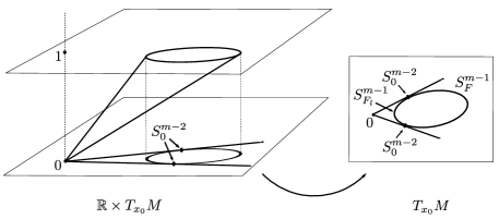
Figure 8. The intersection between the future-pointing light cone at $(t_{0},x_{0})$ and the slice $\{1\}\times T_{x_{0}}M$ projects onto the wind Finslerian structure $\Sigma_{x_{0}}=S_{F}^{m-1}\cup S_{0}^{m-2}\cup S_{F_{l}}^{m-1}$, ($m=2$)

3.4. Projection on $\partial_{t}^{\perp}$ and interpretation of $A_{l}$, $\tilde{A_{l}}$

The fact that the radicand in the expressions of $F$ and $F_{l}$ (formulas (30) and (32)) may not be automatically positive has been interpreted above (possibilities $(c2)$ and $(c3)$ in Corollaries 3.13 and 3.16). Let us go a step further by analysing the metric tensor in this radicand, that is,

$$h:=\Lambda g_{0}+\omega\otimes\omega,$$ (34)

on $M$. The metric $h$ admits the following interpretation on the open subset $M_{\Lambda\neq 0}=\{x\in M:\Lambda\neq 0\}$ where $\partial_{t}$ is not lightlike.

Proposition 3.18.

Let $p_{\mathds{R}}^{\perp}:\mathds{R}\times TM_{\Lambda\neq 0}\rightarrow\mathds{R}\times TM_{\Lambda\neq 0}$ the natural projection on the bundle $\partial^{\perp}_{t}$, $g$-orthogonal to $\partial_{t}$. Then, for any $v\in T_{x}M,x\in M_{\Lambda\neq 0}$:

$$h(v,v)=\Lambda g(p_{\mathds{R}}^{\perp}(0,v),p_{\mathds{R}}^{\perp}(0,v)).$$

Moreover, $h(v,v)/\Lambda^{2}=(F+F^{\hbox{\tiny frev}})^{2}(v)/4$ and, thus, $h/\Lambda^{2}$ is conformally invariant.

Proof.

For the first assertion, apply $g$ to $p_{\mathds{R}}^{\perp}(0,v)=(\omega(v)/\Lambda,v)$. For the last one, use (30) and (32) (or (33)) and recall that Fermat metrics are conformally invariant, Theorem 3.10. ∎

That is, the metric $h$ on $M$ can be identified with a metric conformal to the original one $g$ restricted to $\partial_{t}^{\perp}$, being the conformal factor $\Lambda$ such that $h$ makes sense even in the limit case when $\partial_{t}$ is lightlike. Recall that $\Lambda$ and $\omega$ satisfy (27), then we immediately get:

Corollary 3.19.

The metric $h$ on $M$ is Riemannian when $\Lambda>0$, degenerate when $\Lambda=0$ and it has coindex 1 (i.e., $-h$ is Lorentzian) when $\Lambda<0$.

In the region $M_{l}$ where $\Lambda<0$, the expressions of $F$ and $F_{l}$ (resp. $\tilde{F}$ and $\tilde{F}_{l}$) have been well-defined on all $A_{E}$ (resp. $\tilde{A}_{E}=-A_{E}$) in Convention 2.19. Then, one has directly the following characterizations of the lightlike vectors for $-h$ on $M_{l}$.

Proposition 3.20.

For any $v\in TM_{l}\setminus\mathbf{0}$, the following properties are equivalent:

(i) $h(v,v)=0$, i.e., $v$ is lightlike for the Lorentzian metric $-h$.

(ii) $v$ belongs to the boundary of $A_{E}\cup\tilde{A}_{E}$ in $TM_{l}\setminus\mathbf{0}$,

(iii) either $v\in A_{E}$ and $F(v)=F_{l}(v)$ or $v\in\tilde{A}_{E}$ and $\tilde{F}(v)=\tilde{F}_{l}(v)$, and

(iv) either $v\in A_{E}$ and $F(v)=-\frac{g_{0}(v,v)}{\omega(v)}$ or $v\in\tilde{A}_{E}$ and $\tilde{F}(v)=\frac{g_{0}(v,v)}{\omega(v)}$.

Consistently, the Lorentzian metric $-h$ is time-oriented so that a lightlike vector $v$ for $-h$ will be defined as future-pointing if it belongs to the boundary of $A_{E}$.

Therefore, $A_{l}$ (resp. $\tilde{A}_{l}$) can be interpreted as the set of all the future-pointing (resp. past-pointing) timelike vectors for $-h$; analogously, $A_{E}$ (resp. $\tilde{A}_{E}$) is the set of all the future-pointing (resp. past-pointing) causal vectors.

The following property of lightlike geodesics of $(\mathds{R}\times M,g)$ in terms of $h$ will be useful later. Notice first that if $\gamma=(\zeta,\sigma)$ is a lightlike curve in $(\mathds{R}\times M,g)$ then

$$g(\dot{\gamma},\partial_{t})=-\Lambda\dot{\zeta}+\omega(\dot{\sigma})=\left\{\begin{array}[]{lll}\omega(\dot{\sigma})&&\hbox{if}\,\Lambda=0\\ \mp\sqrt{\Lambda g_{0}(\dot{\sigma},\dot{\sigma})+\omega(\dot{\sigma})^{2}}&&\hbox{if}\,\Lambda\neq 0,\end{array}\right.$$ (35)

(take into account (33)). In particular, the lightlike vectors for $-h$ in the region $M_{l}$ can be interpreted as the projection of lightlike vectors of the spacetime orthogonal to $\partial_{t}$, in addition to the characterizations in Proposition  3.20. Now, recall that if $\gamma$ is a geodesic of $(\mathds{R}\times M,g)$, then $g(\dot{\gamma},\partial_{t})$ is constant along $\gamma$ (as $\partial_{t}$ is Killing).

Lemma 3.21.

For any lightlike geodesic $\gamma=(\zeta,\sigma)$ of $(\mathds{R}\times M,g)$, the constant $C=g(\dot{\gamma},\partial_{t})$ satisfies $C^{2}=h(\dot{\sigma},\dot{\sigma})$. Moreover, if $C=0$ either (i) $\sigma$ is constant, $\sigma\equiv x_{0}\in M$, and the integral curve of $K$ that projects onto $x_{0}$ is a lightlike pregeodesic (that is, $d\Lambda$ vanishes on the kernel of $\omega_{x_{0}}$) or (ii) $\sigma$ remains in the closure $\bar{M}_{l}$ of $M_{l}$ (in particular, if $M_{l}=\emptyset$ this case cannot hold), $\sigma$ can reach the boundary $\partial M_{l}$ only at isolated points (where the $g_{0}$-acceleration $D^{g_{0}}\dot{\sigma}/ds$ does not vanish) and, whenever $\sigma$ remains in $M_{l}$ ($-h$ is Lorentzian on $\sigma$), $\sigma$ is a lightlike geodesic of $h/\Lambda$.

Proof.

For the first assertion, recall that the expression (35) is equal to $\sqrt{h(\dot{\sigma},\dot{\sigma})}$ up to a sign, i.e. $h(\dot{\sigma},\dot{\sigma})=C^{2}$.

For the last assertion, if $\sigma$ is constantly equal to $x_{0}$, then $\gamma$ can be a geodesic if and only if the corresponding orbit of $\partial_{t}$ can be reparametrized as a geodesic. This happens if and only if the gradient $\nabla^{g}\Lambda$ of $\Lambda$ with respect to the metric $g$, when projected on $TM$ by using the differential of $\pi:\mathds{R}\times M\rightarrow M$, is $0$. In fact, since for a Killing vector field $K$, $\nabla^{g}(g(K,K))=-2\nabla_{K}K$, an orbit $\gamma(t)=(t,x_{0})$ of $\partial_{t}$ is a pregeodesic if and only if there exists a function $\lambda$ such that $\nabla^{g}\big{(}g(\partial_{t},\partial_{t})\big{)}|_{(t,x_{0})}=\lambda(t)\partial_{t}|_{(t,x_{0})}$, for all $t\in\mathds{R}$. Recalling that $-g(\partial_{t},\partial_{t})(t,x_{0})=\Lambda(x_{0})$, for all $t\in\mathds{R}$, and that $\omega_{x_{0}}$ is the one-form on $M$ $g_{0}$-equivalent to the $g$-orthogonal projection of $\partial_{t}$ on $TM$, this equation is equivalent to the condition that $\mathrm{d}\Lambda(x_{0})$ is proportional to $\omega_{x_{0}}$, as required.

Finally, observe that a lightlike geodesic $\gamma=(\zeta,\sigma)$ with $\sigma$ non-constant can have $C=0$ only in $\bar{M}_{l}$ and, if there exists some $s_{0}$ such that $\sigma(s_{0}):=x_{0}\in\partial M_{l}$, then: (i) $\dot{\sigma}(s_{0})=0$ (otherwise, $\gamma$ cannot be both, lightlike and orthogonal to $\partial_{t}$), (ii) $d\Lambda_{x_{0}}$ cannot be proportional to $\omega_{x_{0}}$ (otherwise, by uniqueness of geodesics $\gamma$ would be a reparametrization of an integral curve of $\partial_{t}$), and (iii) $\left(D^{g_{0}}\dot{\sigma}/ds)\right)(s_{0})\neq 0$. To see this, observe that $\gamma$ is a geodesic of $(\mathds{R}\times M,g)$ if and only if

$$\frac{D^{g_{0}}}{ds}\dot{\sigma}=-\ddot{\zeta}\,\omega^{\sharp}+\dot{\zeta}\,\hat{\Omega}(\dot{\sigma})-\frac{1}{2}\dot{\zeta}^{2}\,\nabla^{g_{0}}\Lambda,$$

$$\omega(\dot{\sigma})-\Lambda\,\dot{\zeta}={\rm const.}$$

where $D^{g_{0}}/ds$ and $\nabla^{g_{0}}$ are respectively the covariant derivative of $(M,g_{0})$ along $\sigma$ and the gradient with respect to $g_{0}$, $\omega^{\sharp}$ is the vector field $g_{0}$-equivalent to $\omega$ and $g_{0}(w,\hat{\Omega}(v))={\rm d}\omega(v,w)$ for every $v,w\in TM$. The above equations can be obtained for example using that the geodesics are the critical points of the energy functional (or using the explicit formulas (13) and (14) in [38], which are valid for arbitrary $\Lambda$). Then $\left(\frac{D^{g_{0}}}{ds}\dot{\sigma}\right)(s_{0})\not=0$ because otherwise $\ddot{\zeta}(s_{0})\,\omega^{\sharp}_{x_{0}}=-\frac{1}{2}\dot{\zeta}^{2}(s_{0})\,\nabla^{g_{0}}\Lambda(x_{0})$. As $\dot{\zeta}^{2}(s_{0})\neq 0$, because $\gamma$ is lightlike, we conclude that $\sigma$ is constant by $(i)$. Now, in the region $M_{l}$, the map $\pi:(\mathds{R}\times M_{l},g)\rightarrow(M_{l},h/\Lambda)$ is a semi-Riemannian submersion (see Proposition 3.18) and therefore, lightlike geodesics orthogonal to the fibers project into (and are all the lifts of) lightlike geodesics of $(M_{l},h/\Lambda)$. ∎

Stationary spacetimes have been studied in many mathematically oriented papers, see e.g. [39, 66, 50, 38, 21, 42, 23, 18], while the case $\Lambda\equiv 0$, which includes global Brinkmann decompositions [14], has been considered recently in [6], where the authors study geodesic connectedness.

3.5. Fundamental tensors for $F,F_{l}$

Recall that when $\Lambda>0$, $F$ is a Randers metric with a well-known positive definite fundamental tensor (see for example [51, Corollary 4.17]) and, when $\Lambda=0$, then $F$ is a Kropina metric with also a positive-definite fundamental tensor (see [51, Corollary 4.12]). Next, we focus on the region $\Lambda<0$ and the domain $A_{l}$ of $TM$.

The fundamental tensors of $F$ and $F_{l}$ can be computed explicitly from the expressions (30) and (32) by taking into account that these metrics can be regarded as canonical $(F_{0},\omega)$-ones, i.e. they can be written as $F_{0}\cdot\phi(\omega/F_{0})$ being $F_{0}$ the root of $g_{0}$ and

$$\phi(z)=\frac{1}{-z\pm\sqrt{z^{2}+\Lambda}},$$

see [51, §4.2.1]. In any case, a simplified computation can be accomplished. In fact, it is enough to study the fundamental tensor of the Randers type metrics:

$$F^{\epsilon}=-\epsilon\sqrt{\tilde{h}}+\beta\quad\quad\hbox{with}\;\tilde{h}=\beta\otimes\beta-\bar{g}_{0},$$

where $\beta$ is the one-form $\omega/\Lambda$, and $\bar{g}_{0}$ the Riemannian metric $g_{0}/|\Lambda|$, so that $\tilde{h}$ is Lorentzian with coindex $1$ and $\beta(v)>0$ on $A_{l}$. The value of $\epsilon$ is $1$ for $F$ and $-1$ for $F_{l}$.

Proposition 3.22.

Let $G^{\epsilon},\epsilon=\pm 1$, be the fundamental tensor of $F^{\epsilon}$, i.e., of $F$ for $\epsilon=1$ and $F_{l}$ for $\epsilon=-1$. Then, with the above notation for $\tilde{h}$ and $\beta$:

$$G^{\epsilon}_{v}(w,w)=-\epsilon F^{\epsilon}(\tilde{v})\left(\tilde{h}(w,w)-\tilde{h}(\tilde{v},w)^{2}\right)+\left(-\epsilon\tilde{h}(\tilde{v},w)+\beta(w)\right)^{2}$$ (36)

for all $v\in A_{l}$ and $w\in T_{x_{0}}M$, where $\tilde{v}=v/\sqrt{\tilde{h}(v,v)}$ on $A_{l}$.

Proof.

It is enough to observe that [51, Prop. 4.10], with $\phi(s)=-\epsilon+s$, holds also in this case. ∎

Remark 3.23.

Observe that (36) can be used to prove directly that $F$ and $F_{l}$ are, respectively, conic Finsler and Lorentzian Finsler in their domains $A$ and $A_{l}$. Focusing on $A_{l}$, clearly $G^{\epsilon}_{v}(v,v)=F^{\epsilon}(v)^{2}>0$; therefore, the space of the vectors $u\in T_{x_{0}}M$ which are $G^{\epsilon}_{v}$-orthogonal to $v$ is transversal to $v$ and has dimension $m-1$. Moreover, setting $v\in A_{l}$:

$$G^{\epsilon}_{v}(v,u)=0\quad\Leftrightarrow\quad\beta(u)=\epsilon\tilde{h}(\tilde{v},u)\quad\quad\quad\left(\Leftrightarrow\beta(u)=-\frac{\epsilon\bar{g}_{0}(\tilde{v},u)}{1-\epsilon\beta(\tilde{v})}\right).$$

By using repeatedly this equivalence, if $u$ is $G_{v}$-orthogonal to $v$, (36) becomes:

$$G^{\epsilon}_{v}(u,u)=-\epsilon F^{\epsilon}(\tilde{v})\left(\tilde{h}(u,u)-\tilde{h}(\tilde{v},u)^{2}\right)=\epsilon F^{\epsilon}(\tilde{v})\bar{g}_{0}(u,u),$$

and the result follows as $F^{\epsilon}(\tilde{v})>0$.

4. The case of causal $K$: Randers-Kropina metrics

Next, we focus on the case of an $\rm SSTK$ splitting when $K$ is causal (i.e., $\Lambda\geq 0$), so that its Fermat structure becomes a Randers-Kropina metric $F$ according to Definition 2.59. In particular, $A_{l}=\emptyset$, and $A_{x}=T_{x}M\setminus\{0\}$ iff $\Lambda(x)>0$ while $A_{x}$ is an open half-space in $T_{x}M$ iff $\Lambda(x)=0$ (recall Definition 2.11 and Proposition 3.12). Therefore, $F_{l}$ and $A_{E}$ will not be used and we will consider $F$-admissibility rather than notions as wind curves —the wind balls will be also treated in a way similar to the classical Finslerian one. Our aim is to show that, on the one hand, $F$ can be used to describe the causality of the spacetime $(\mathds{R}\times M,g)$ and, on the other hand, the known properties on causality of spacetimes allow us to obtain properties of the associated Finslerian separation $d_{F}:M\times M\rightarrow[0,+\infty]$.

4.1. Characterization of the chronological relation

Following [51, Definitions 3.6, 3.8], for any conic pseudo-Finsler metric $F\colon A\subseteq TM\to[0,+\infty)$ on $M$ and any $x,y\in M$, one says that $x$ $F$-precedes $y$, written $x\prec y$, if there is an $F$-admissible curve from $x$ to $y$. Here, a curve is said $F$-admissible consistently with Definition 2.20, i.e., if its velocity lies in the domain $A$ of $F$, so that $x\prec y$ iff $\Omega^{A}_{x,y}\neq\emptyset$. We recall that the Finslerian separation $d_{F}$ (Definition 2.24) is non-negative and satisfies a triangle inequality, namely, $d(x,z)\leq d(x,y)+d(y,z)$ for all $x,y,z\in M$, but it is non-symmetric and $d_{F}(x,x)$ can be positive [51, Proposition 3.9]; in the case that a standard Finsler metric is regarded as the conic Finsler metric of a wind Finslerian structure $\Sigma$, the balls $B_{F}^{+}(x,r)$ and $B_{F}^{-}(x,r)$ introduced in Definition 2.24 agree with the wind balls $B_{\Sigma}^{+}(x,r)$ and $B_{\Sigma}^{-}(x,r)$ of $\Sigma$ (see Definition 2.26 and notice that $F_{l}=+\infty$ in this case). Both of them are open subsets and constitute a basis for the topology of $M$ in the standard Finsler case and these properties are generalizable to the wind Finslerian case (recall Proposition 2.25). However, the closures $\bar{B}_{F}^{\pm}(x,r)$ of these balls cannot be obtained merely replacing the strict equalities by non-strict ones (see Corollary 4.8 below).

Now, let us focus on the $F$-separation $d_{F}$ of the conic Finsler metric $F$ associated with an $\rm SSTK$ splitting with $K$ causal. The chronological relation can be characterized in a simple way.

Proposition 4.1.

For any $\rm SSTK$ splitting with causal $K$:

$$(t_{0},x_{0})\ll(t_{1},x_{1})\quad\Leftrightarrow\quad d_{F}(x_{0},x_{1})<t_{1}-t_{0},$$

for every $x_{0},x_{1}\in M$ and $t_{0},t_{1}\in\mathds{R}$. Therefore:

$$\begin{array}[]{l}I^{+}(t_{0},x_{0})=\{(t,y):d_{F}(x_{0},y)<t-t_{0}\},\\ I^{-}(t_{0},x_{0})=\{(t,y):d_{F}(y,x_{0})<t_{0}-t\}.\end{array}$$ (37)

Equivalently, considering $d_{F}$-forward and backward balls

$$I^{+}(t_{0},x_{0})=\cup_{s>0}\{t_{0}+s\}\times B_{F}^{+}(x_{0},s),\quad I^{-}(t_{0},x_{0})=\cup_{s>0}\{t_{0}-s\}\times B_{F}^{-}(x_{0},s).$$

Proof.

Recall that a vector $(\tau,v)\in\mathds{R}\times TM$ is timelike and future-pointing if and only if $\tau>F(v)$ (see Corollary 3.13 cases (a) and (b)).

If $(t_{0},x_{0})\ll(t_{1},x_{1})$, then there exists a future-pointing timelike curve $\gamma=(t,\sigma):[0,1]\rightarrow\mathds{R}\times M$ from $(t_{0},x_{0})$ to $(t_{1},x_{1})$ such that $\dot{t}>F(\dot{x})$ and, perturbing the curve when needed, we can assume that $\dot{x}(s)\not=0$ for every $s\in[0,1]$ Then by integration, we get $t_{1}-t_{0}>\ell_{F}(\sigma)$, i.e. $d_{F}(x_{0},x_{1})<t_{1}-t_{0}$.

Conversely, if $d_{F}(x_{0},x_{1})<t_{1}-t_{0}$, choose an $F$-admissible curve $\sigma:[0,1]\rightarrow M$ from $x_{0}$ to $x_{1}$ such that $d_{F}(x_{0},x_{1})\leq\ell_{F}(\sigma)<t_{1}-t_{0}$. Then the curve $(t,\sigma):[0,1]\rightarrow\mathds{R}\times M$, where $t(s)=t_{0}+\ell_{F}(\sigma|_{[0,s]})+\varepsilon s$ and $\varepsilon=t_{1}-t_{0}-\ell_{F}(\sigma)$, is a timelike future-pointing curve from $(t_{0},x_{0})$ to $(t_{1},x_{1})$.

The remainder is then straightforward. ∎

4.2. Continuity of the Finslerian separation for Randers-Kropina spaces

Let us start with a general result.

Proposition 4.2.

The $F$-separation associated with any conic pseudo-Finsler metric $F$ is upper semi-continuous, i.e., if $x_{n}\rightarrow x$, $y_{n}\rightarrow y$, then

$$\limsup_{n}d_{F}(x_{n},y_{n})\leq d_{F}(x,y).$$

In particular, if $x\prec y$, then $x_{n}\prec y_{n}$ for large $n$.

Proof.

Assume that $d_{F}(x,y)<+\infty$ and, by contradiction,

$$d_{F}(x_{n},y_{n})>d_{F}(x,y)+3\varepsilon$$

for some $\varepsilon>0$ and for some subsequences still denoted by $x_{n}$ and $y_{n}$. Choose a curve $\gamma$ from $x$ to $y$ with $\ell_{F}(\gamma)<d_{F}(x,y)+\varepsilon$ and choose $\bar{x},\bar{y}$ on $\gamma$ such that $x\in B_{F}^{-}(\bar{x},\varepsilon)$ and $y\in B_{F}^{+}(\bar{y},\varepsilon)$. By [51, Prop. 3.9] these two balls are open and so, for large $n$, they contain all $x_{n}$ and $y_{n}$. So, the curve $\rho$ obtained by concatenating an $F$-admissible curve of length smaller than $\varepsilon$ from $x_{n}$ to $\bar{x}$ with the piece of $\gamma$ from $\bar{x}$ to $\bar{y}$ and with another $F$-admissible curve of length smaller than $\varepsilon$ from $\bar{y}$ to $y_{n}$ yields the required contradiction $d_{F}(x_{n},y_{n})<d_{F}(x,y)+3\varepsilon$. ∎

Although lower semi-continuity may not hold even in the conic Finsler case (and even with points $x,y$ at a finite $F$-separation, see [51, Example 3.18]), we will check that this semi-continuity does hold in the Randers-Kropina case.

Notice first the following straightforward consequence of Proposition 4.1.

Proposition 4.3.

For any $\rm SSTK$ splitting with causal $K$, the function

$$\tau_{F}:M\times M\rightarrow[0,+\infty],\quad\quad\tau_{F}(x,y):=\inf\{t\in\mathds{R}:\,(0,x)\ll(t,y)\}$$

is equal to the $F$-separation function $d_{F}$.

The function $\tau_{F}$ will be called the (future) arrival time function and its definition on $M$ instead of $\mathds{R}\times M$ uses implicitly the invariance of the metric with $t$.

Next, we will prove the lower semi-continuity of $d_{F}$ by using results of spacetimes (which, in particular, extend those in [78]). To this aim, we will use a well-known result on limit curves. The latter are defined as follows (see [8, Definition 3.28]).

Definition 4.4.

A curve $\gamma$ in a spacetime $(L,g)$ is a limit curve of a sequence of curves $\{\gamma_{k}\}$, if there exists a subsequence $\{\gamma_{m}\}$ such that for all $p$ in the image of $\gamma$, any neighborhood of $p$ intersects all but a finite number of the curves in $\{\gamma_{m}\}$.

A standard result says that any sequence $\{\gamma_{k}\}$ of causal, future-pointing, future-inextendible causal curves whose images have an accumulation point $p$ admits a limit curve through $p$ which is also causal, future-pointing and future-inextendible (see [8, Proposition 3.31]; the same holds replacing “future” with “past” in the previous statement). Let us remark that a limit curve is not necessarily piecewise smooth, but causal continuous (for the definition of a causal continuous curve see the beginning of §3.2 in [8]). Moreover, observe that to be causal continuous on an interval $I$ is equivalent to be locally absolutely continuous with future-pointing causal derivative a. e. in $I$ (see [17, Theorem A.1]).

Theorem 4.5.

The $F$-separation $d_{F}:M\times M\rightarrow[0,+\infty]$ associated with any Randers-Kropina metric is continuous away from the diagonal $D=\{(x,x):x\in M\}\subset M\times M$.

Proof.

From Proposition 4.3 and Proposition 4.2, it is enough to prove the lower semi-continuity of $\tau_{F}$ for the corresponding $\rm SSTK$ splitting.

Let $\{x_{n}\}$ and $\{y_{n}\}$ be converging sequences, $x_{n}\to x,y_{n}\to y\neq x$, and assume by contradiction that there exist subsequences, denoted again by $\{x_{n}\}$, $\{y_{n}\}$, such that $\{\tau_{F}(x_{n},y_{n})\}$ converges with

$$T_{0}:=\lim_{n}\tau_{F}(x_{n},y_{n})<\tau_{F}(x,y).$$

Choose $T_{1}\in(T_{0},\tau_{F}(x,y))$, and define $q_{n}:=(T_{1},y_{n})$, $p_{n}:=((T_{1}-T_{0})/2,x_{n})$. Each line $l_{y_{n}}=\{(s,y_{n}):s\in\mathds{R}\}$ is causal and, since $\tau_{F}(x_{n},y_{n})$ is finite for large $n$, necessarily $p_{n}\ll q_{n}$ for $n$ big enough (recall $l_{y}\neq l_{x}$ and Remark 3.1). Thus, we can take a sequence of past-pointing timelike curves $\{\gamma_{n}\}$ connecting each $q_{n}$ with $p_{n}$. Moreover, these curves are assumed to be inextendible to the past, by prolonging them with the lines $l_{x_{n}}$. As $\{q_{n}\}\rightarrow q_{\infty}:=(T_{1},y)$, the sequence $\{\gamma_{n}\}$ admits a causal, past-inextendible and past-pointing limit curve $\gamma$ starting at $q_{\infty}$. Necessarily, $\gamma$ must leave $l_{y}$ at some point $Q$; otherwise, as $\gamma$ is inextendible, it must run all $(t,q_{\infty})$ when $t\rightarrow-\infty$ (but this is absurd because the points in $\gamma$ lie in the closure of the set of images of all $\gamma_{n}$, and the piece of such curves with $t\circ\gamma_{n}\leq(T_{1}-T_{0})/2$ lie in $l_{x_{n}}$, which accumulate at $l_{x}\neq l_{y}$). Notice also that if $\gamma$ arrived at the limit $p_{\infty}:=((T_{1}-T_{0})/2,x)$ of $\{p_{n}\}$, a contradiction with the definition of $\tau_{F}(x,y)$ would be obtained. Now, choose $T_{2}\in(T_{1},\tau_{F}(x,y))$ and any point $Q^{\prime}$ on $\gamma$ away from $l_{y}$; necessarily $Q^{\prime}<Q<(T_{2},y)$ and, then, $Q^{\prime}\ll(T_{2},y)$ (recall Remark 3.1). But $Q^{\prime}$ lies in the closure of the images of the set of all $\gamma_{n}$ and, thus, up to a subsequence, some point $Q^{\prime}_{n}$ on each $\gamma_{n}$ satisfies $Q^{\prime}_{n}\ll(T_{2},y)$ for large $n$. Therefore, we can assume

$$p_{n}(\ll Q^{\prime}_{n})\ll(T_{2},y),$$

and choose a future-inextendible timelike curve $\alpha_{n}$ from $p_{n}$ to $(T_{2},y)$ and equal to $l_{y}$ beyond this point. Consider the limit curve $\alpha$ of the sequence $\alpha_{n}$ departing from $p_{\infty}$. Reasoning as above, $\alpha$ leaves $l_{x}$ at some point, and any point $Q^{\prime\prime}$ on $\alpha$ away from $l_{x}$ satisfies $p=(0,x)\ll Q^{\prime\prime}$. Choose a point $Q^{\prime\prime}_{n}$, in a curve $\alpha_{n}$, close enough to $Q^{\prime\prime}$ such that $p\ll Q^{\prime\prime}_{n}$. This concludes that

$$p\ll Q^{\prime\prime}_{n}\ll(T_{2},y),$$

in contradiction with the definition of $\tau_{F}(x,y)$. ∎

The necessity of the exception on the diagonal $D$ in the previous theorem comes from the following fact.

Proposition 4.6.

The $F$-separation $d_{F}$ associated with a Randers-Kropina metric is discontinuous at $(x_{0},x_{0})$ if $d_{F}(x_{0},x_{0})>0$. Moreover,

• the property $d_{F}(x_{0},x_{0})>0$ occurs if there exists a neighborhood $U$ of $x_{0}$ such that no admissible loop contained in $U$ exists, i.e. $y\not\prec_{U}y$, for all $y\in U$; in particular for any Kropina metric $F=\alpha^{2}/\beta$ such that the kernel of $\beta$ is locally integrable, i.e. $\beta\wedge d\beta=0$;

• for any Kropina norm on a vector space, $d_{F}(x,x)=\infty$ for all $x\in V$.

Proof.

For the first assertion, choosing any $F$-admissible curve $\gamma$ starting at $x$, one constructs trivially a sequence $\{x_{n}\}$, $x_{n}\rightarrow x$ of points on $\gamma$ with $d_{F}(x,x_{n})\rightarrow 0$. For (i), notice that any $F$-admissible loop starting at $x$ (and leaving necessarily $U$) will have a length greater than some $\varepsilon>0$; to check this, notice that one can always obtain a Finsler metric $F_{0}$ in any compact neighborhood of $x$ such that $F_{0}$ is smaller than $1$ on the indicatrix of $F$. In the Kropina case, the assumption $\beta\wedge d\beta=0$ implies that $\beta|_{U}=\Omega df$ on a small neighborhood $U$ of $x_{0}$, for a positive function $\Omega$ and $f$ with no critical points on $U$ (as any Kropina metric is defined only on the open region of the manifold $M$ where $\beta$ is nowhere vanishing). So $f$ is strictly increasing on any admissible curve on $U$ (recall that $\beta(v)>0$ for $v\in A$); thus, $y\not\prec_{U}y$ for all $y\in U$. Finally in the case of a Kropina norm, being $\beta$ a constant one-form, $\beta=df$ on $V$ and therefore $d_{F}(x,x)=\infty$ for all $x\in V$. ∎

Remark 4.7.

The previous proposition shows that explicit examples of discontinuous $d_{F}$ can be constructed easily. It also shows that the possible discontinuity on the diagonal would not be removed if $d_{F}(x,x)$ were redefined as $0$ (namely, regarding $\tau_{F}(x,y)$ as the infimum of the set $\{t\in\mathds{R}:(0,x)\leq(t,y)\}$ and defining $d_{F}(x,y)$ as the new $\tau_{F}(x,y)$). On the other hand, it is trivial to check that for any Randers-Kropina metric $F$, if $K$ is timelike at $x\in M$ then $d_{F}(x,x)=0$ and $d_{F}$ is continuous at $(x,x)$.

Finally notice the discontinuity of $d_{F}$ at the diagonal yields the following subtlety (consistent with Definition 2.26 and Proposition 2.33).

Corollary 4.8.

The closed forward (resp. backward) $d_{F}$-balls, defined as the closures of the corresponding open balls, satisfy, for $r>0$:

$$\bar{B}_{F}^{+}(x,r)=\{y\in M:d_{F}(x,y)\leq r\}\cup\{x\}$$

$$\hbox{(resp.}\;\bar{B}_{F}^{-}(x,r)=\{y\in M:d_{F}(y,x)\leq r\}\cup\{x\}).$$

Proof.

The proof of the first assertion in the previous proposition shows that $\{x\}$ belongs to the closure of the ball. So, just apply the continuity of $d_{F}$ outside the diagonal. ∎

4.3. Ladder of causality and properties for Randers-Kropina separation

Next, we can go further into the causal structure of our class of spacetimes. The following relation between the position of the spacetime in the causal ladder and the properties of the Randers-Kropina metric appears.

Theorem 4.9.

Consider an $\rm SSTK$ splitting $(\mathds{R}\times M,g)$ as in (26) with $K$ causal and associated Randers-Kropina metric $F$ on $M$. Then, $(\mathds{R}\times M,g)$ is causally continuous, and

1. the following assertions are equivalent:

   (i1) $(\mathds{R}\times M,g)$ is causally simple i.e., it is causal (which means that no closed smooth causal curve exists) and the sets $J^{+}(p)$, $J^{-}(p)$ are closed for all $p\in\mathds{R}\times M$).

   (i2) $(M,F)$ is convex, in the sense that for every $x,y\in M$, $x\neq y$, with $d_{F}(x,y)<+\infty$, there exists a geodesic $\gamma$ from $x$ to $y$ such that $\ell_{F}(\gamma)=d_{F}(x,y)$.

   (i3) $J^{+}(p)$ is closed for all $p\in\mathds{R}\times M$.

   (i4) $J^{-}(p)$ is closed for all $p\in\mathds{R}\times M$.

2. $(\mathds{R}\times M,g)$ is globally hyperbolic (i.e. it is causal and all the intersections $J^{+}(p)\cap J^{-}(q)$ are compact) if and only if $\bar{B}_{F}^{+}(x,r_{1})\cap\bar{B}_{F}^{-}(y,r_{2})$ is compact (or empty) for every $x,y\in M$ and $r_{1},r_{2}>0$.

3. The following assertions are equivalent:

   (iii1) A slice $S_{t}=\{(t,x):x\in\mathds{R}\times M\}$ (and, then all the slices) is a spacelike Cauchy hypersurface i.e., it is crossed exactly once by any inextendible timelike curve (and, then, also by any causal one).

   (iii2) the closures $\bar{B}_{F}^{+}(x,r)$, $\bar{B}_{F}^{-}(x,r)$ are compact for all $r>0$ and $x\in M$.

   (iii3) $F$ is forward and backward geodesically complete.

Proof.

First observe that, as $t:\mathds{R}\times M\rightarrow\mathds{R}$, $(t,x)\mapsto t$, is a temporal function, then $(\mathds{R}\times M,g)$ is stably causal and, in particular, distinguishing (for the elements of causality to be used here, see [71] or [8, 12]). So, to prove causal continuity, it is enough to show that $(\mathds{R}\times M,g)$ is future and past reflecting (see for example [71, Definition 3.59, Lemma 3.46] or [8, Theorem 3.25, Proposition 3.2]). Let us see that it is past reflecting (the other case is analogous), that is, $I^{+}(p)\supset I^{+}(q)$ implies $I^{-}(p)\subset I^{-}(q)$ for any $p=(t_{0},x)$ and $q=(t_{1},y)$. We can assume $x\neq y$ (otherwise it is obvious), and the inclusion $I^{+}(p)\supset I^{+}(q)$ implies that $d_{F}(x,y)\leq t_{1}-t_{0}$. This is a consequence of the continuity of $d_{F}$ away from $D$ proven in Theorem 4.5. In fact, consider a sequence $\{q_{n}=(t_{1}+\varepsilon_{n},y_{n})\}$ contained in $I^{+}(q)$ and converging to $q$ so that $\varepsilon_{n}\searrow 0,y_{n}\rightarrow y$. By (37), $d_{F}(x,y_{n})<(t_{1}-t_{0})+\varepsilon_{n}$, and, by the continuity of $d_{F}$, the required inequality holds. But $d_{F}(x,y)\leq t_{1}-t_{0}$ implies directly $I^{-}(p)\subset I^{-}(q)$ (use again (37) and the triangle inequality for $d_{F}$), as required.

Equivalences in $(i)$ and $(ii)$ can be proved formally as in the stationary case [23]. The proof of the equivalences in $(iii)$ has some differences with respect to the stationary case due to the lack of a Hopf-Rinow theorem for Randers-Kropina metrics. The reader can check, however, that both, the equivalence between (iii1) and (iii3), and the implications (iii1) $\Rightarrow$ (iii2) $\Rightarrow$ (iii3) hold by means of simple modifications of the arguments in [23, Theorems 4.3 and 4.4]. In any case, a full proof can be obtained as a particular case of the most general Theorem 5.9 below. ∎

As a straightforward consequence of Theorem 4.9 and the implications from causality theory (iii1) $\Rightarrow$ global hyperbolicity $\Rightarrow$ (i1), one has the following version of Hopf-Rinow theorem.

Corollary 4.10.

For any Randers-Kropina metric $F$ on a manifold $M$, the forward (resp. backward) geodesic completeness of $d_{F}$ is equivalent to the compactness of the forward closed balls $\bar{B}^{+}_{F}(x,r)$ (resp. backward closed balls $\bar{B}^{-}_{F}(x,r)$) for every $x\in M,r>0$. Moreover, any of these properties implies the compactness of the intersection between any pair of forward and backward closed balls. Finally, the last property implies the convexity of $(M,F)$, in the sense of Theorem 4.9.

Example 4.11.

The so-called Brinkmann spaces are defined by the existence of a complete parallel lightlike vector field $K$, and they include many physical examples of interest, as wave-type spacetimes (plane waves, pp-waves etc.); a detailed study of these spaces is carried out in [14]. Under very general hypotheses, they are strongly causal [37] and become an $\rm SSTK$ [33, Th. V.11]; so, they determine a Kropina metric where all the previous results are applicable. We mention that they have been considered recently in [6], where their geodesic connectedness is studied.

5. The case of arbitrary $K$: general wind Riemannian structures

In this section we consider the general case of a Killing vector field $K$ with no restriction on its pointwise causal character.

5.1. Causal futures and lightlike geodesics

For the study of the causality of a general $\rm SSTK$ splitting, we will use its Fermat structure $\Sigma$ in Definition 3.9 and the notation for causal elements in Section 3.1.

We start with a characterization of the chronological relation which generalizes the one obtained in Proposition 4.1 when $K$ is causal; notice that there is now no natural Finslerian separation that fully describes the causal properties of $(\mathds{R}\times M,g)$. This problem will be circumvented by means of a description of the causal futures and pasts, which makes apparent an interpretation of the c-balls. Recall that the time coordinate of the $\rm SSTK$ splitting is a temporal function and every causal curve can be parametrized with the time.

Proposition 5.1.

Let $(\mathds{R}\times M,g)$ be an $\rm SSTK$ splitting. Then:

$$I^{+}(t_{0},x_{0})=\cup_{s>0}\{t_{0}+s\}\times B_{\Sigma}^{+}(x_{0},s),$$

$$I^{-}(t_{0},x_{0})=\cup_{s>0}\{t_{0}-s\}\times B_{\Sigma}^{-}(x_{0},s),$$

$$J^{+}(t_{0},x_{0})=\cup_{s\geq 0}\{t_{0}+s\}\times\hat{B}_{\Sigma}^{+}(x_{0},s),$$

$$J^{-}(t_{0},x_{0})=\cup_{s\geq 0}\{t_{0}-s\}\times\hat{B}_{\Sigma}^{-}(x_{0},s).$$

Proof.

Taking into account Corollary 3.13 and Convention 2.19, a vector $(\tau,v)\in\mathds{R}\times(TM\setminus\mathbf{0})$ with $\tau>0$ is causal and future-pointing if and only if $v\in A_{E}\cup A\setminus\mathbf{0}$ and

$$F(v)\leq\tau\leq F_{l}(v);$$ (38)

moreover, it is timelike and future-pointing if and only if both inequalities hold strictly in (38) (and, thus, $v\in A$). Accordingly, a $t$-parametrized piecewise smooth curve $(t,x):[t_{0},t_{1}]\rightarrow\mathds{R}\times M$ is causal (resp. timelike) and future-pointing if and only if $x$ is $\Sigma$-admissible and

$$F(\dot{x}(t))\leq\dot{t}\equiv 1\leq F_{l}(\dot{x}(t))$$ (39)

(resp. $x$ is $F$-admissible and

$$F(\dot{x}(t))<\dot{t}\equiv 1<F_{l}(\dot{x}(t)))$$ (40)

thus, in particular, $x$ is a wind curve. Now, reasoning for the future and the inclusions $\subset$, observe that if $(t_{1},x_{1})\in J^{+}(t_{0},x_{0})$, then there exists a future-pointing causal curve $\gamma=(t,x)$ joining $(t_{0},x_{0})$ and $(t_{1},x_{1})$, with $x$ being $\Sigma$-admissible (recall footnote 6) . So, integrating in (39) one has: if $(t_{1},x_{1})\in J^{+}(t_{0},x_{0})$ then $x_{1}\in\hat{B}^{+}_{\Sigma}(x_{0},t_{1}-t_{0})$ (resp. if $(t_{1},x_{1})\in I^{+}(t_{0},x_{0})$, then $x_{1}\in B^{+}_{\Sigma}(x_{0},t_{1}-t_{0})$), as required.

For the converse $\supset$, in the case $J^{+}$, choose any $x_{1}\in\hat{B}^{+}_{\Sigma}(x_{0},s)$ and a wind curve $x:[0,s]\rightarrow M$ from $x_{0}$ to $x_{1}$ such that $\ell_{F}(x)\leq s\leq\ell_{F_{l}}(x)$ (which exists by definition of $\hat{B}_{\Sigma}(x_{0},s)$). From (39), the curve $[t_{0},t_{0}+s]\ni t\mapsto(t,x(t-t_{0}))$ is the required causal curve from $(t_{0},x_{0})$ to $(t_{0}+s,x_{1})$. Moreover, to check the inclusion $\supset$ for $I^{+}$, notice that if $x_{1}\in B^{+}_{\Sigma}(x_{0},s)$ then the inequalities (39) hold strictly at some point. If both of them hold at some point $\bar{t}$, then the causal curve becomes timelike at $(\bar{t},x(\bar{t}-t_{0}))$ —so that the points $(t_{0},x_{0})$ and $(t_{0}+s,x_{1})$ can be connected by means of a timelike curve, see for example [72, Proposition 10.46]. Otherwise, there must exist two disjoint intervals $[\bar{t}_{1},\bar{t}_{2}]$, $[\bar{t}_{3},\bar{t}_{4}]\subset]0,s]$ such that in $[\bar{t}_{1},\bar{t}_{2}]$ does hold the second strict inequality and in $[\bar{t}_{3},\bar{t}_{4}]$ it holds the first one. Assume that $\bar{t}_{2}<\bar{t}_{3}$ (the other case is analogous) and define the function

$$\rho(\mu)=\begin{cases}0&0\leq\mu\leq\bar{t}_{1}\\ \varepsilon(\mu-\bar{t}_{1})&\bar{t}_{1}\leq\mu\leq\bar{t}_{2}\\ \varepsilon(\bar{t}_{2}-\bar{t}_{1})&\bar{t}_{2}\leq\mu\leq\bar{t}_{3}\\ \varepsilon\left(\bar{t}_{2}-\bar{t}_{1}+\frac{\bar{t}_{2}-\bar{t}_{1}}{\bar{t}_{4}-\bar{t}_{3}}(\bar{t}_{3}-\mu)\right)&\bar{t}_{3}\leq\mu\leq\bar{t}_{4}\\ 0&\bar{t}_{4}\leq\mu\leq s\end{cases}$$

If $\varepsilon>0$ is small enough, the curve $[0,s]\ni\mu\mapsto(\mu+\rho(\mu),x(\mu))\in\mathds{R}\times M$ is a causal curve from $(t_{0},x_{0})$ to $(t_{0}+s,x_{1})$ which is timelike in some point. Then applying again [72, Proposition 10.46] we conclude. ∎

We recall that two points $p$ and $q$ in a spacetime are said horismotically related if $q\in J^{+}(p)\setminus I^{+}(p)$. We will give a characterization of these points after the following lemma.

Lemma 5.2.

Let $I\subset\mathds{R}$ be an interval and $\rho\colon I\rightarrow\mathds{R}\times M$ be a lightlike future-pointing pregeodesic of an $\rm SSTK$ splitting $(\mathds{R}\times M,g)$. Then $\rho$ can be reparametrized as $s\mapsto(s,x(s))$ on $[t(\rho(a)),t(\rho(b))]$ and the function $C_{\rho}(s):=g(\partial_{t},\dot{\rho}(s))$ either has a definite sign on $I$ or it vanishes everywhere.

Proof.

The possibility of the reparametrization follows because the projection $t:\mathds{R}\times M\rightarrow\mathds{R}$ is a temporal function (see part (1) of Remark 3.4). Moreover, since $\partial_{t}$ is a Killing vector field, $g(\partial_{t},\dot{\gamma})$ is constant for any geodesic $\gamma$ of $(\mathds{R}\times M,g)$, which implies that $g(\partial_{t},\dot{\rho}(s))$ will preserve the sign in $s\in I$, as $\rho$ is a reparametrization of a geodesic of $(\mathds{R}\times M,g)$. ∎

Corollary 5.3.

Two distinct points $(t_{0},x_{0}),(t_{1},x_{1})\in\mathds{R}\times M$ are horismotically related if and only if $x_{1}\in\hat{B}^{+}_{\Sigma}(x_{0},t_{1}-t_{0})\setminus B^{+}_{\Sigma}(x_{0},t_{1}-t_{0})$.

In this case, there exists a lightlike pregeodesic $\rho:[t_{0},t_{1}]\rightarrow\mathds{R}\times M$, $\rho(s)=(s,x(s))$ from $(t_{0},x_{0})$ to $(t_{1},x_{1})$ and such that $x$ is a unit extremizing geodesic of $\Sigma$ from $x_{0}$ to $x_{1}$ with $\ell_{F}(x)=t_{1}-t_{0}$ or $\ell_{F_{l}}(x)=t_{1}-t_{0}$ (or both). Moreover, when $x$ is a constant curve (i.e. an extremizing exceptional geodesic), necessarily $\Lambda(x_{0})=0$ with $\mathrm{d}\Lambda(\mathrm{Ker}\,\omega_{x_{0}})\equiv 0$; when $x$ is not constant then it is regular (in the sense of Definition 2.20-(iii)).

Proof.

The first equivalence is straightforward from Proposition 5.1. More precisely, two horismotically related points are connected by a lightlike geodesic $\gamma$ (see e.g. [72, Proposition 10.46]) and, applying Lemma 5.2, we can reparametrize $\gamma$ as $\rho(s)=(s,x(s))$. Now, $x$ is a wind curve connecting $x_{0}$ with $x_{1}$, and horismoticity implies $x(s)\in\hat{B}^{+}_{\Sigma}(x_{0},s-t_{0})\setminus B^{+}_{\Sigma}(x_{0},s-t_{0})$, for all $s\in(t_{0},t_{1}]$, so that $x$ is a unit extremizing geodesic (Definition 2.35). The last assertions follow from Lemmas 3.21 and 5.2. ∎

The next result characterizes the lightlike geodesics of an $\rm SSTK$ spacetime in terms of the Finslerian elements. But, first, the following lemma points out some simple technical properties. Recall that a Lorentzian manifold $(M,g)$ admits a convex neighborhood $U$ at every point $p\in M$ (i.e., $U$ is a normal neighborhood of all its points), [88].

Lemma 5.4.

Given an $\rm SSTK$ splitting $(\mathds{R}\times M,g)$ and $z_{0}=(t_{0},x_{0})\in\mathds{R}\times M$ there exists a convex neighborhood $U$ of $z_{0}$, a neighborhood $V$ of $z_{0}$ contained in $U$ and some small $\varepsilon>0$ such that $J^{+}(z)\cap\{(t,x)\in\mathds{R}\times M:t\in[t(z),t_{0}+\varepsilon)\}\subset U$ for every $z\in V$.

Proof.

Consider a chart $(U,y^{0},y^{1},\ldots,y^{m})$ around $z_{0}$ such that no causal curve starting at $U$ will leave and return to $U$ (this can be obtained as the $\rm SSTK$ spacetime is strongly causal, Remark 3.4 (1)) and with the coordinates adapted to the product structure ($y^{0}=t$, $y^{1},...y^{m}$ coordinates on $M$). Choosing a smaller $U$, such that it is convex in $(\mathds{R}\times M,g)$, define a (flat) Minkowski metric $g^{\text{\tiny flat}}$ in these coordinates such that $\partial_{i},\ i\in\{1,\ldots,m\},$ span a spacelike hyperplane and the timecones of $g^{\text{\tiny flat}}$ are wider than those of $g$ (this can be obtained obviously at the point $z_{0}$ and, by continuity, in some small neighborhood). Then, the required property for $g$ holds as it does trivially for $g^{\text{\tiny flat}}$. ∎

Theorem 5.5.

Let $I\subset\mathds{R}$ be an interval and $\rho(s)=(s,x(s)),\ s\in I$, be a (piecewise smooth) curve in an $\rm SSTK$ splitting $(\mathds{R}\times M,g)$. Then $\rho$ is a future-pointing lightlike pregeodesic of $(\mathds{R}\times M,g)$ if and only if its projection $I\ni s\to x(s)\in M$ is a unit geodesic of $(M,\Sigma)$. Moreover, in this case:

1. $C_{\rho}<0$ iff $x$ is a unit geodesic of $F$ ($F(\dot{x})\equiv 1$; $x$ is $F$-admissible).

2. $C_{\rho}>0$ iff $x$ is a unit geodesic of $F_{l}$ ($F_{l}(\dot{x})\equiv 1$; $x$ is $F$-admissible).

3. $C_{\rho}=0$ iff one of the following two possibilities occurs:

   (a) $\rho$ is an integral curve of $K$ which projects onto some $x_{0}$ with $\Lambda(x_{0})=0$ and $\mathrm{d}\Lambda(\mathrm{Ker}\,\omega_{x_{0}})\equiv 0$ (so that the projection is an exceptional geodesic, Definition 2.44), or

   (b) $x$ is contained in $\overline{M}_{l}$; whenever it remains included in $M_{l}$, $x$ is a lightlike pregeodesic of $-h$ parametrized with $F(\dot{x})\equiv F_{l}(\dot{x})\equiv 1$, and $x$ can reach $\partial M_{l}$ only at isolated points $s_{j}\in I,j=1,2...$, where $\Lambda(x(s_{j}))=0$, $\dot{x}(s_{j})=0$ and $\left(D^{g_{0}}\dot{x}/ds\right)(s_{j})\neq 0$.

Proof.

Assume that $\rho$ is a lightlike pregeodesic. For each $s_{0}\in I$ (different from its endpoints, and with straightforward modifications otherwise), there exists $\varepsilon>0$ such that $[s_{0}-\varepsilon,s_{0}+\varepsilon]\subset I$ and $\rho(s)\in J^{+}(\rho(s_{0}-\varepsilon))\setminus I^{+}(\rho(s_{0}-\varepsilon))$, for all $s\in[s_{0}-\varepsilon,s_{0}+\varepsilon]$ (recall, for example, [72, Proposition 5.34] and use strong causality). Thus, Corollary 5.3 can be applied locally (recall Lemma 5.4), and $x|_{[s_{0}-\varepsilon,s_{0}+\varepsilon]}$ is a unit extremizing geodesic of the Fermat structure $(M,\Sigma)$.

Conversely, if $x:I\rightarrow M$ is a unit geodesic of $(M,\Sigma)$, then it is locally a unit extremizing geodesic (recall Definitions 2.44, 2.35). So, by Proposition 5.1, every $s_{0}$ (as above) admits an $\varepsilon>0$ such that $[s_{0}-\varepsilon,s_{0}+\varepsilon]\subset I$ and the curve $[s_{0}-\varepsilon,s_{0}+\varepsilon]\ni s\rightarrow(s,x(s))\in\mathds{R}\times M$ is contained in $J^{+}(s_{0}-\varepsilon,x(s_{0}-\varepsilon))\setminus I^{+}(s_{0}-\varepsilon,x(s_{0}-\varepsilon))$; therefore, it is a lightlike pregeodesic (see [72, Proposition 10.46]).

For the last part, first notice that $C_{\rho}=-\Lambda(x(s))+\omega(\dot{x}(s))$ and $C^{2}_{\rho}=h(\dot{x},\dot{x})$ (the latter follows as in the first part of the proof of Lemma 3.21). Thus, when $C_{\rho}\neq 0$, $\dot{x}(s)$ belongs to $A_{x(s)}$, for all $s\in I$. Hence, $x$ is a unit and $F$-admissible geodesic of $(M,\Sigma)$ and, then, from Theorem 2.53, a geodesic of $F$ or $F_{l}$. Precisely, from part $(iii)$ of Proposition 3.12, $F(\dot{x})=1$ iff $-C_{\rho}=\Lambda(x(s))-\omega(\dot{x}(s))\geq 0$ and $F_{l}(\dot{x})=1$ iff $-C_{\rho}=\Lambda(x(s))-\omega(\dot{x}(s))\leq 0$, i.e. $x$ is a unit $F$-geodesic iff $C_{\rho}<0$ and a unit $F_{l}$-geodesic iff $C_{\rho}>0$. Finally, $(iii)$ follows from Lemma 3.21. ∎

As a straightforward consequence of Lemmas 3.21, 5.2 and Theorem 5.5 we get:

Corollary 5.6.

Let $\gamma\colon I\to\mathds{R}\times M$, $\gamma(s)=(\zeta(s),\sigma(s))$ be a (piecewise smooth) curve in an $\rm SSTK$ splitting $(\mathds{R}\times M,g)$, with $\sigma$ non-constant. Then $\gamma$ is a future-pointing lightlike geodesic if and only if $\sigma$ is a pregeodesic of $(M,\Sigma)$ parametrized with $h(\dot{\sigma},\dot{\sigma})=\mathrm{const.}$, and one of the following three exclusive possibilities holds

1. $C_{\gamma}<0$ and $\sigma$ is a pregeodesic of $F$ and $\zeta(\bar{s}_{0})-\zeta(s_{0})=\ell_{F}(\sigma|_{[s_{0},\bar{s}_{0}]})$ for any $s_{0},\bar{s}_{0}\in I$, $s_{0}<\bar{s}_{0}$;

2. $C_{\gamma}>0$ and $\sigma$ is a pregeodesic of $F_{l}$ and $\zeta(\bar{s}_{0})-\zeta(s_{0})=\ell_{F_{l}}(\sigma|_{[s_{0},\bar{s}_{0}]})$ for any $s_{0},\bar{s}_{0}\in I$, $s_{0}<\bar{s}_{0}$;

3. $C_{\gamma}=0$, $\sigma$ is smooth, it is included in $\overline{M}_{l}$, it touches $\partial M_{l}$ at most at isolated points $s_{j}$, $j=1,2,\ldots,$ such that $\dot{\sigma}(s_{j})=0$, $\sigma$ is a lightlike geodesic of $h/\Lambda$ whenever it remains in $M_{l}$, and also $\zeta$ is determined by

   $$\zeta(\bar{s}_{0})-\zeta(s_{0})=\ell_{F_{l}}(\sigma|_{[s_{0},\bar{s}_{0}]})=\ell_{F}(\sigma|_{[s_{0},\bar{s}_{0}]})$$

   for any $s_{0},\bar{s}_{0}\in I$, $s_{0}<\bar{s}_{0}$.

5.2. Characterization of the causal ladder

The following technical property concerns limit curves (recall Definition 4.4) in connection with time functions. The role of these functions in the limit process is not usually taken into account (indeed, it is rather trivial in the case of Cauchy temporal functions). So, we write it for any stably causal spacetime, which may have interest in its own right.

Lemma 5.7.

Let $(L,g)$ be a spacetime endowed with a time function $t:L\rightarrow\mathds{R}$.

1. Consider a sequence of inextendible causal curves $\{\gamma_{n}\}$ parametrized by the time $t$ and assume that there exists a convergent sequence $\{t_{n}\}$ such that $\gamma_{n}(t_{n})$ converges to $z_{0}$. Then there exists an (inextendible, causal) limit curve $\gamma$ through $z_{0}$ parametrized by the time $t$, and a subsequence $\gamma_{n_{k}}$ such that, whenever the intersection of $\gamma$ with the slice $S_{t_{0}}:=\{z\in L:t(z)=t_{0}\}$ is not empty for $t_{0}\in\mathds{R}$, then all the curves $\gamma_{n_{k}}$ but a finite number intersect $S_{t_{0}}$ and $\gamma(t_{0})=\lim_{k}\gamma_{n_{k}}(t_{0})$.

2. Let $\gamma_{n}$ be a sequence of causal curves and, for each $n\in\mathds{N}$, $z_{n}\leq w_{n}$ be two points on $\gamma_{n}$. If $z_{n}\to z$, $w_{n}\to w$, $z\neq w$, and the intersection of the slice $S_{t_{0}}$ with the images of all $\gamma_{n}$ lies in a compact subset for any $t_{0}\in(t(z),t(w))$, then any (inextendible) limit curve $\gamma$ of the sequence starting at $z$ arrives at $w$.

Proof.

$(i)$ The existence of the limit curve follows from [8, Proposition 3.31]. Let $\{\gamma_{n_{k}}\}$ be any subsequence that converges to $\gamma$ uniformly on compact subsets for some auxiliary complete Riemannian metric (up to a reparametrization, according to [8, Lemma 14.2]) and, so, such that some sequence $\{p_{k}:=\gamma_{n_{k}}(t_{n_{k}})\},t_{n_{k}}\in\mathds{R}$, converges to $p:=\gamma(t_{0})$; in particular $t_{n_{k}}\rightarrow t_{0}$. Choose open neighborhoods $V,U$ of $p$, with $V\subset U$, $U$ convex and $V$ having compact closure included in $U$ and being globally hyperbolic with Cauchy hypersurface $S_{t_{0}}$. Due to the convergence to $p$, all $\gamma_{n_{k}}$ but a finite number will enter in $V$ and cross $V\cap S_{t_{0}}$ at a single point $q_{k}$. Reasoning by contradiction, if $\{q_{k}\}$ does not converge to $p$ then, up to a subsequence, $\{q_{k}\}$ converges to some $q\in U\setminus\{p\}$. Assume that, up to a new subsequence, $p_{k}\leq q_{k}$ (otherwise we could assume $q_{k}\leq p_{k}$ up to a subsequence, and the reasoning would be analogous). By the convexity of $U$, $p\leq q$ but, as $p$ and $q$ lie in the acausal set $V\cap S_{t_{0}}$, one obtains the absurd $p=q$.

$(ii)$ Let $t^{*}\in(t(z),t(w))$ and let us reparameterize all the curves with $t$. Assume that $\gamma:[t(z),t^{*})\rightarrow L$ cannot be extended to $t^{*}$. Let $\{\gamma_{n_{k}}\}$ be any subsequence that converges to $\gamma$ as in part $(i)$ and such that $\{\gamma_{n_{k}}(t^{*})\}$ converges to some point $z^{*}\in S_{t^{*}}$, the latter property by the assumption on compactness. Up to a subsequence, $\{\gamma_{n_{k}}\}$ admits a limit curve starting at $z^{*}$, say, $\rho:(t^{*}-\varepsilon,t^{*}]\rightarrow L$ for some $\varepsilon>0$. Now, by part $(i)$, necessarily $\{\gamma_{n_{k}}(t)\}$ converges to both $\gamma(t)$ and $\rho(t)$, for each $t\in(t^{*}-\varepsilon,t^{*})$. So, $\gamma$ admits $z^{*}$ as a future limit point and it is then extendible, a contradiction. Thus, $\gamma$ is defined on $[t(z),t(w))$ and since $w_{n}\to w$ necessarily it arrives at $w$. ∎

As a first consequence, we obtain characterizations of some causal properties, which will be related to the possible reflectivity and causal simplicity of the spacetime.

Proposition 5.8.

For any $p=(t_{0},x_{0}),q=(t_{1},x_{1})$ in an $\rm SSTK$ splitting:

1. $I^{+}(p)\supset I^{+}(q)$ if and only if $x_{1}\in\bar{B}^{+}_{\Sigma}(x_{0},t_{1}-t_{0})$, and

2. $I^{-}(p)\subset I^{-}(q)$ if and only if $x_{0}\in\bar{B}^{-}_{\Sigma}(x_{1},t_{1}-t_{0})$.

Moreover,

$$\bar{J}^{+}(t_{0},x_{0})=\left(\cup_{s>0}\{t_{0}+s\}\times\bar{B}_{\Sigma}^{+}(x_{0},s)\right)\,\cup\,\{(t_{0},x_{0})\}$$

$$\bar{J}^{-}(t_{0},x_{0})=\left(\cup_{s>0}\{t_{0}-s\}\times\bar{B}_{\Sigma}^{-}(x_{0},s)\right)\,\cup\,\{(t_{0},x_{0})\}$$

Proof.

We consider the case $(i)$, being part $(ii)$ analogous.

($\Rightarrow$) Choose $\{q_{n}\}\subset I^{+}(q)$, converging to $q$ and inextendible future-pointing timelike curves $\gamma_{n}$ through $p$ and $q_{n}$. From part $(i)$ of Lemma 5.7, there exists a subsequence $\gamma_{n_{k}}$ that cuts the slice $S_{t_{1}}$ in a sequence of points $(t_{1},y_{n_{k}})$, such that $y_{n_{k}}\to x_{1}$. By Proposition 5.1, $y_{n_{k}}\in B^{+}_{\Sigma}(x_{0},t_{1}-t_{0})$ and, then, $x_{1}\in\bar{B}^{+}_{\Sigma}(x_{0},t_{1}-t_{0})$.

($\Leftarrow$) As $x_{1}\in\bar{B}^{+}_{\Sigma}(x_{0},t_{1}-t_{0})$, take a sequence $\{\tilde{y}_{n}\}$ in $B^{+}_{\Sigma}(x_{0},t_{1}-t_{0})$ converging to $x_{1}$. The sequence $q_{n}=(t_{1},\tilde{y}_{n})$ converges to $q$ and, by Proposition 5.1, is contained in $I^{+}(p)$. As the chronological relations are open, given $r\in I^{+}(q)$, then $r\in I^{+}(q_{n})$ for $n$ big enough. This implies that $r\in I^{+}(p)$ and then $I^{+}(p)\supset I^{+}(q)$, as required.

For the last assertion, recall first that, in any spacetime $\bar{J}^{\pm}(p)=\bar{I}^{\pm}(p)$ (see, e.g. [72, Lemma 14.6]) hence the inclusions $\supset$ hold trivially from Proposition 5.1. For the converse in the case of $\bar{J}^{+}$, let $q=(t_{1},x_{1})\in\bar{J}^{+}(p)=\bar{I}^{+}(p)$, and take $q_{n}\in I^{+}(p)$ such that $q_{n}\to q$. Apply part $(i)$ of Lemma 5.7 to obtain a sequence $(t_{1},y_{n_{k}})\in I^{+}(p)$ such that $y_{n_{k}}\to x_{1}$, and conclude again from Proposition 5.1 that $y_{n_{k}}\in B^{+}_{\Sigma}(x_{0},t_{1}-t_{0})$, so that $x_{1}\in\bar{B}^{+}_{\Sigma}(x_{0},t_{1}-t_{0})$. ∎

Now, we can study the causal ladder of any $\rm SSTK$ splitting, extending the Randers-Kropina case in Theorem 4.9.

Theorem 5.9.

Consider an $\rm SSTK$ splitting $(\mathds{R}\times M,g)$ as in (26) with associated Fermat structure $\Sigma$ on $M$. Then, $(\mathds{R}\times M,g)$ is stably causal and

1. $(\mathds{R}\times M,g)$ is causally continuous if and only if $\Sigma$ satisfies the following property: given any pair of points $x_{0},x_{1}$ in $M$ and $r>0$, $x_{1}\in\bar{B}^{+}_{\Sigma}(x_{0},r)$ if and only if $x_{0}\in\bar{B}^{-}_{\Sigma}(x_{1},r)$.

2. $(\mathds{R}\times M,g)$ is causally simple if and only if $(M,\Sigma)$ is w-convex (according to Definition 2.45).

3. The following assertions are equivalent:

   1. $(\mathds{R}\times M,g)$ is globally hyperbolic.

   2. $\hat{B}^{+}_{\Sigma}(x,r_{1})\cap\hat{B}^{-}_{\Sigma}(y,r_{2})$ is compact for every $x,y\in M$ and $r_{1},r_{2}>0$.

   3. $\bar{B}^{+}_{\Sigma}(x,r_{1})\cap\bar{B}^{-}_{\Sigma}(y,r_{2})$ is compact for every $x,y\in M$ and $r_{1},r_{2}>0$.

4. The following assertions are equivalent:

   1. A slice $S_{t}$ (and, then every slice) is a spacelike Cauchy hypersurface.

   2. All the c-balls $\hat{B}_{\Sigma}^{+}(x,r)$ and $\hat{B}_{\Sigma}^{-}(x,r)$, $r>0$, $x\in M$, are compact.

   3. All the (open) balls $B_{\Sigma}^{+}(x,r)$ and $B_{\Sigma}^{-}(x,r)$, $r>0$, $x\in M$, are precompact.

   4. $\Sigma$ is forward and backward geodesically complete (according to Definition 2.45).

Proof.

$(i)$ As the natural projection $t:\mathds{R}\times M\rightarrow\mathds{R}$ is a temporal function, Remark 3.4, the spacetime is stably causal. Thus, causal continuity becomes equivalent to past and future reflectivity. However, by Proposition 5.8, past reflectivity (i.e., $I^{+}(p)\supset I^{+}(q)$ implies $I^{-}(p)\subset I^{-}(q)$) becomes equivalent to the property

$$x_{1}\in\bar{B}^{+}_{\Sigma}(x_{0},t_{1}-t_{0})\Rightarrow x_{0}\in\bar{B}^{-}_{\Sigma}(x_{1},t_{1}-t_{0}),$$

and future reflectivity is equivalent to the converse.

$(ii)$ Assuming that $(\mathds{R}\times M,g)$ is causally simple, for any $x_{0}\in M$ and $t_{0}<t_{1}$, the intersections $S_{t_{1}}\cap J^{+}(t_{0},x_{0})$ and $S_{2t_{0}-t_{1}}\cap J^{-}(t_{0},x_{0})$ must be closed. By Proposition 5.1, these intersections are equal to $\{t_{1}\}\times\hat{B}_{\Sigma}^{+}(x_{0},t_{1}-t_{0})$ and $\{2t_{0}-t_{1}\}\times\hat{B}_{\Sigma}^{-}(x_{0},t_{1}-t_{0})$, respectively, which means that $\Sigma$ is w-convex. For the converse, just apply the last assertion of Proposition 5.8, plus Proposition 2.33 and Proposition 5.1.

$(iii)$ ($(iii1)\Rightarrow(iii2)$) Assume that $(\mathds{R}\times M,g)$ is globally hyperbolic and consider the points $(r_{1},x)$ and $(-r_{2},y)$. By Proposition 5.1,

$$\{0\}\times\left(\hat{B}_{\Sigma}^{+}(x,r_{1})\cap\hat{B}_{\Sigma}^{-}(y,r_{2})\right)=(\{0\}\times M)\cap J^{+}(-r_{1},x)\cap J^{-}(r_{2},y),$$

and the right-hand side is compact by global hyperbolicity.

($(iii2)\Rightarrow(iii3)$) By Proposition 2.33, it is enough to prove that the property of compactness of the intersections implies the closedness of the c-balls. Reasoning by contradiction, if, say, $z\in\bar{B}_{\Sigma}^{+}(x,r_{1})\setminus\hat{B}_{\Sigma}^{+}(x,r_{1})$, as $z$ always belongs to some (open) ball ${B}_{\Sigma}^{-}(y,r_{2})$ (recall that one can take any $\Sigma-$ admissible curve through $z$ in order to choose appropriate $y$ and $r_{2}$), necessarily $\hat{B}_{\Sigma}^{+}(x,r_{1})\cap\hat{B}_{\Sigma}^{-}(y,r_{2})$ cannot be compact.

($(iii3)\Rightarrow(iii1)$) For any $(t_{0},x_{0})$, $(t_{1},x_{1})$ in $\mathds{R}\times M$, recalling Propositions 5.1 and 2.33, we get

$$J^{+}(t_{0},x_{0})\cap J^{-}(t_{1},x_{1})\subset$$

$$\cup_{s\in(0,t_{1}-t_{0})}\{t_{0}+s\}\times\left(\bar{B}_{\Sigma}^{+}(x_{0},s)\cap\bar{B}_{\Sigma}^{-}(x_{1},t_{1}-t_{0}-s)\right)\,\cup\,\{(t,x_{0}),(t_{1},x_{1})\}$$

and we have to check that the left-hand side is compact. Indeed, for any sequence $\{z_{n}\}\subset J^{+}(t_{0},x_{0})\cap J^{-}(t_{1},x_{1})$ we can take a sequence of causal curves $\gamma_{n}$ from $(t_{0},x_{0})$ to $(t_{1},x_{1})$ passing through $z_{n}$. By the hypothesis on the closures, part $(ii)$ of Lemma 5.7 is applicable, and there exists a limit curve $\gamma$ of $\{\gamma_{n}\}$ with the same endpoints. So, some subsequence $\{\gamma_{n_{k}}\}$ converges in the $C^{0}$ topology to $\gamma$ (see [8, Proposition 3.34]) and, thus, $\{z_{n_{k}}\}$ lies in a compact subset, admitting so a convergent subsequence to a point in the image of $\gamma$.

$(iv)$ ($\it(iv1)\Rightarrow(iv2)$) By Proposition 5.1,

$$J^{+}(0,x)\cap S_{r}=\{r\}\times\hat{B}_{\Sigma}^{+}(x,r),\quad J^{-}(0,x)\cap S_{-r}=\{-r\}\times\hat{B}_{\Sigma}^{-}(x,r)$$

and the left-hand sides are compact as $S_{r},S_{-r}$ are Cauchy hypersurfaces (otherwise, the limit curve of the sequence of causal curves obtained by connecting $(0,x)$ with a diverging sequence of points would not cross the corresponding Cauchy hypersurface).

($\it(iv2)\Rightarrow(iv3)$) Just apply Proposition 2.33.

($\it(iv3)\Rightarrow(iv1)$) By using the one-parameter group of isometries generated by the complete Killing field $\partial_{t}$, one easily sees that if a slice $S_{t_{0}}$ is a Cauchy hypersurface then all the slices $S_{t}$ are Cauchy hypersurfaces. Thus, by contradiction, let us assume that $S_{0}$ is not Cauchy. Hence, there will exist some inextendible timelike curve $\rho:[0,t_{0})\rightarrow\mathds{R}\times M$, $\rho(s)=(s-t_{0},x_{\rho}(s))$ or $\rho:(-t_{0},0]\rightarrow\mathds{R}\times M$, $\rho(s)=(s+t_{0},x_{\rho}(s))$, which does not cross it. We recall that any timelike vertical line $s\mapsto(s,\bar{x})$, $\bar{x}\in M$, always crosses once $S_{0}$ and that, for any subinterval $[s_{1},s_{2}]\subset[0,t_{0})$ (or $\subset(-t_{0},0]$) containing some point $\bar{s}$ where $\dot{x}_{\rho}(\bar{s})=0$, $\rho_{|[s_{1},s_{2}]}$ can be replaced by a timelike future-pointing curve $\tilde{\rho}(s)=(s,x_{\tilde{\rho}}(s))$, such that $\dot{x}_{\tilde{\rho}}(s)\neq 0$, for each $s\in[s_{1},s_{2}]$ (see footnote 6). Summing up, we can assume, without losing generality, that $\dot{x}_{\rho}(s)\neq 0$, for all $s$. Thus, being $\rho$ timelike and future-pointing, we have (recall (40)) $\ell_{F}(x_{\rho})<t_{0}<\ell_{F_{l}}(x_{\rho})$. Then if $\epsilon>0$ is small enough, $x_{\rho}(t_{0}-\epsilon)\in B_{\Sigma}^{+}(x_{\rho}(0),t_{0})$ or $x_{\rho}(-t_{0}+\epsilon)\in B_{\Sigma}^{-}(x_{\rho}(0),t_{0})$. As $\rho$ cannot remain in a compact region of the spacetime (otherwise it would be extendible), either $B_{\Sigma}^{+}(x_{\rho}(0),t_{0})$ in the first case, or $B_{\Sigma}^{-}(x_{\rho}(0),t_{0})$ in the second one, is not precompact.

($\it(iv1)\Leftrightarrow(iv4)$) As the slices $S_{t}$ are closed, spacelike and acausal, each one will be Cauchy if and only if it is crossed by any future-pointing inextendible lightlike pregeodesic $\rho$ (see [72, Lemma 14.42 and Corollary 14.54]). So, let $\rho$ be any inextendible future-pointing lightlike pregeodesic and let us parametrize it as $\rho(s)=(s,x_{\rho}(s))$ (recall Lemma 5.2). Hence, $S_{t}$ will be Cauchy if and only if $\rho$ is defined on $\mathds{R}$. From the first part of Theorem 5.5, this property is equivalent to saying that $(M,\Sigma)$ is forward and backward geodesically complete. ∎

Remark 5.10.

(1) As suggested by the equivalence $(i)$ above, wind Finslerian structures where $x_{1}\in\bar{B}^{+}_{\Sigma}(x_{0},r)$ does not imply that $x_{0}\in\bar{B}^{-}_{\Sigma}(x_{1},r)$ do exist (in contrast with the Randers-Kropina case); in fact, it is not difficult to construct explicit examples, as the one in Fig. 9.

(2) In the comparison with the Randers-Kropina case, notice that Theorem 4.9 was stated by using only balls for the Finslerian separation $d_{F}$, as this notion had familiar similarities with a distance. However, the results stated here in terms of c-balls are more accurate and refine those in that theorem.

Figure 9. A wind Finslerian structure on $\mathds{R}^{2}$ minus the bold dashed segment, where $x_{1}\in\bar{B}^{+}_{\Sigma}(x_{0},r)$ but $x_{0}\not\in\bar{B}^{+}_{\Sigma}(x_{1},r)$

6. Applications to wind Riemannian structures and navigation

As emphasized in Section 3, every wind Riemannian structure can be seen as the Fermat structure of a certain $\rm SSTK$ splitting (canonically chosen in a conformal class, see Theorem 3.10), which will be referred to as the $\rm SSTK$ splitting associated with the wind Riemannian structure.

Along this section, some results on wind Riemannian structures will be obtained by using the associated $\rm SSTK$ splitting. Some of these properties can be generalizable to any wind Finslerian structure, see Section 9.

6.1. Characterization of geodesics and Hopf-Rinow properties

One of the most relevant difficulties of arbitrary wind Finslerian structures in comparison with standard Finsler (or Riemannian) metrics is that the exponential map is not necessarily defined in all directions. Indeed, the second order differential equations defining the extremizing geodesics of the conic non-degenerate pseudo-Finsler metrics $F$ and $F_{l}$ associated with $\Sigma$ have coefficients $\Gamma^{k}_{\,\,ij}$ defined on a subset ($A$ or $A_{l}$) of $TM$ that, in general, does not contain a punctured neighborhood of the zero section (the most we could say was Theorem 2.53). In wind Riemannian structures, however, this difficulty can be overcome easily by using the associated $\rm SSTK$ splitting. Indeed, recall that a triple $(g_{0},\omega,\Lambda)$ is associated with any wind Riemannian structure $(M,\Sigma)$ (Proposition 2.55 and Definition 2.56) and then an $\rm SSTK$ spacetime with Fermat structure $\Sigma$ (Theorem 3.10). As a first result in this direction we have the following.

Proposition 6.1.

Let $(M,\Sigma)$ be a wind Riemannian manifold, then its wind balls are open.

Proof.

From Proposition 5.1, $B_{\Sigma}^{\pm}(x_{0},s)$ is homeomorphic to $I^{\pm}(t_{0},x_{0})\cap S_{t_{0}+s}$ and, in any spacetime, $I^{\pm}(t_{0},x_{0})$ is open. ∎

Notice that the Lorentzian result [72, Proposition 10.46]) claimed in the proof of Proposition 5.1 has been crucial.

We pass now to study geodesics of a wind Riemannian structure. As any lightlike geodesic is locally horismotic, Corollary 5.3 plus the crucial Lemma 3.21 on lightlike geodesics of an $\rm SSTK$ splitting imply:

Proposition 6.2.

All the non-exceptional geodesics of a wind Riemannian manifold $(M,\Sigma)$ are regular. Moreover, if $x$ is a non-exceptional geodesic of $\Sigma$ then it is a smooth curve, its velocity can be zero only at isolated points and its acceleration (for one auxiliary Riemannian metric and, then, for any of them) does not vanish at those zeroes.

The following theorem characterizes wind Riemannian geodesics and refines Theorem 2.53.

Theorem 6.3.

Let $(M,\Sigma)$ be a wind Riemannian structure. For any $\Sigma$-admissible (piecewise smooth) curve $x:[a,b]\rightarrow M$, the following conditions are equivalent:

1. $x$ is a unit geodesic of $\Sigma$,

2. $x$ satisfies one of the following three exclusive possibilities:

   (a) $x$ is a unit $F$-admissible geodesic of $(M,F)$ and, then, locally, it minimizes the $F$-length

   (b) $x$ is a unit $F$-admissible geodesic of $(M_{l},F_{l})$ and, then, locally, it maximizes the $F_{l}$-length,

   (c) $x$ is a smooth curve contained in $\overline{M}_{l}$ and either (c1) $x$ is constant, $\Lambda(x)=0$ and $d\Lambda({\rm ker}\,\omega_{x})\equiv 0$ or (c2) whenever it remains included in $M_{l}$, $x$ is a lightlike pregeodesic of the Lorentzian metric $-h$ in (34) parametrized with $F(\dot{x})\equiv F_{l}(\dot{x})\equiv 1$ ($x$ is a boundary geodesic), and $x$ can reach $\partial M_{l}$ only at isolated points $s_{j}\in I,j=1,2...$, where $\dot{x}(s_{j})=0$, $d\Lambda({\rm ker}\,\omega_{x(s_{j})})\neq 0$ and its second derivative (in one and then any coordinates) does not vanish.

Proof.

The implication $(i)\Rightarrow(ii)$ follows by applying Theorem 5.5 to the $\rm SSTK$ splitting $(\mathds{R}\times M,g)$ associated with $(M,\Sigma)$. Moreover, as in Theorem 2.53, it can be proved that the extremal properties hold for any variation. For the converse, in the cases $(a)$ and $(b)$, choose $s_{0}\in[a,b]$ and take the future-pointing lightlike geodesic $\gamma$ of the associated $\rm SSTK$ spacetime $(\mathds{R}\times M,g)$, satisfying the initial conditions $\big{(}(s_{0},x(s_{0})),(1,\dot{x}(s_{0}))\big{)}$. Let us reparametrize $\gamma$ as $\rho(s)=(s,x_{\rho}(s))$. From Theorem 5.5, $x_{\rho}$ is a unit geodesic of $(M,\Sigma)$ and, as the vector $\dot{x}(s_{0})\in A_{x(s_{0})}$, $C_{\rho}\neq 0$. Thus, $x_{\rho}$ is, according to the sign of $C_{\rho}$, a unit $F$-admissible geodesic for $F$ or $F_{l}$ which coincides with $x$ by existence and uniqueness of geodesic of a conic pseudo-Finsler metric. In the remaining case $(c)$, whenever $x$ is not constant, $j=1,2,\ldots,$ such that $\Lambda(x_{\rho}(s_{j}))=0$ and $\dot{x}_{\rho}(s_{j})=0$, the curve $\rho(s)=(s,x(s))$ is orthogonal to the Killing vector field (recall part $(iii)$ of Proposition 3.12) and then a lightlike pregeodesic whenever $x$ is contained in $M_{l}$ (recall, from Proposition 3.18, that $\pi:(\mathds{R}\times M_{l},g)\rightarrow(M_{l},\frac{1}{\Lambda}h)$ is a semi-Riemannian submersion, and also that lightlike pregeodesics were preserved by conformal changes of the metric); moreover, as $x$ is smooth and its derivative vanishes at the points where it touches the boundary $\partial M_{l}$, we conclude that $\rho$ is globally a lightlike pregeodesic. Then, from Theorem 5.5-(iii), $x$ is a unit geodesic of $(M,\Sigma)$. Finally, if $x\equiv x_{0}\in M$, $\Lambda(x_{0})=0$ and $d\Lambda({\rm ker}\,\omega_{x_{0}})=0$, then $x$ is an exceptional geodesic of $(M,\Sigma)$. ∎

Lemma 6.4.

For every neighborhood $W_{0}$ of $x_{0}\in M$, there exists another neighborhood $U_{0}\subset W_{0}$ and some $\varepsilon>0$ such that $\hat{B}^{\pm}_{\Sigma}(x,r)$ is compact and contained in $W_{0}$ for every $r<\varepsilon$ and $x\in U_{0}$.

Proof.

The proof is a refinement of Lemma 5.4 obtained by taking into account that, given $W_{0}$ and considering the $\rm SSTK$ splitting $(\mathds{R}\times M,g)$ associated with the wind Riemannian structure, then the convex neighborhood $U$ provided by that lemma around $z_{0}=(0,x_{0})$ can be easily chosen satisfying the following properties: (i) $U$ is included in $\mathds{R}\times W_{0}$, (ii) $U$ is precompact and (iii) $U$ contains the intersections $J^{\pm}(z)\cap([-\varepsilon,\varepsilon]\times M)$ for some $\varepsilon>0$ and all $z$ in a smaller neighborhood $V\subset U$. Then, put $U_{0}:=V\cap S_{0}\subset W_{0}$ and observe that, for any $r\in(0,\varepsilon)$, the set $J^{+}(0,x)\cap(\{\pm r\}\times M)$ is compact for all $x\in U_{0}$ (observe that it is a closed set, as $U$ is normal, included in a compact set, also by hypothesis on $U$) and, by Proposition 5.1, it projects homeomorphically into $\hat{B}^{\pm}_{\Sigma}(x_{0},r)$ and this projection is contained in $W_{0}$ as required. ∎

The following local properties can also be proved by using the spacetime viewpoint. They are equivalent to saying that the exponential maps of the conic pseudo-Finsler metrics associated with a wind Riemannian metric are defined in some small cone.

Proposition 6.5.

Let $(M,\Sigma)$ be a wind Riemannian structure and $x_{0}\in M$, then there exists $\varepsilon>0$ such that the geodesics of $F$ (resp. $F_{l}$) departing from $x_{0}$ and parametrized by the arc length are defined on $[0,\varepsilon)$ and they are extremizing unit geodesic and therefore minima (resp. maxima) of $\ell_{F}$ (resp. $\ell_{F_{l}}$) with respect to any variation.

Proof.

Let $\varepsilon>0$ as in Lemma 6.4 and consider the $\rm SSTK$ splitting associated with $(M,\Sigma)$. Any geodesic $x\colon[0,a_{x}]\to M$, $a_{x}>0$ of $F$ or $F_{l}$, starting at $x_{0}$ and parametrized by the arc length, defines a lightlike pregeodesic $(s,x(s))$ (recall Theorems 5.5 and 6.3) which must be defined on $[0,r]$, for any $r<\varepsilon$. In fact, $(s,x(s))\in J^{+}(0,x_{0})\cap(\{s\}\times M)$ and, for $s\in[0,r]$, $J^{+}(0,x_{0})\cap(\{s\}\times M)$ is contained in a precompact convex neighborhood of $(0,x_{0})$ (see the proof of Lemma 6.4). Therefore, $(s,x(s))\in J^{+}(0,x_{0})\setminus I^{+}(0,x_{0})$ and $x$ must also be an extremizing unit geodesic for $\Sigma$ by Corollary 5.3 and then, being $F$-admissible, it must be a local minimum of $\ell_{F}$ or a local maximum of $\ell_{F_{l}}$ (recall Theorem 6.3). ∎

Finally, the following result becomes straightforward from Theorem 5.9 and plays the role of Hopf-Rinow theorem for wind Finslerian structures (then generalizing Corollary 4.10).

Proposition 6.6.

Let $(M,\Sigma)$ be a wind Riemann structure.

1. The following properties are equivalent:

   1. $\Sigma$ is geodesically complete,

   2. $B^{+}_{\Sigma}(x,r)$ and $B^{-}_{\Sigma}(x,r)$ are precompact for every $x\in M$ and $r>0$.

   3. $\hat{B}^{+}_{\Sigma}(x,r)$ and $\hat{B}^{-}_{\Sigma}(x,r)$ are compact for every $x\in M$ and $r>0$.

   In particular, if $M$ is compact then $\Sigma$ is geodesically complete.

2. The following properties are equivalent and imply the w-convexity (Definition 2.45) of $(M,\Sigma)$:

   1. $\hat{B}^{+}_{\Sigma}(x,r_{1})\cap\hat{B}^{-}_{\Sigma}(y,r_{2})$ is compact for every $x,y\in M$ and $r_{1},r_{2}>0$.

   2. $\bar{B}^{+}_{\Sigma}(x,r_{1})\cap\bar{B}^{-}_{\Sigma}(y,r_{2})$ is compact for every $x,y\in M$ and $r_{1},r_{2}>0$.

   Moreover, these conditions hold whenever the previous ones in $(i)$ are satisfied.

3. If $(M,\Sigma)$ is w-convex, then $x_{1}\in\bar{B}^{+}_{\Sigma}(x_{0},r)$ if and only if $x_{0}\in\bar{B}^{-}_{\Sigma}(x_{1},r)$ for any $x_{0},x_{1}\in M$ and $r>0$.

Proof.

Apply Theorem 5.9 to the associated $\rm SSTK$ splitting (see Theorem 3.10), and use the causal implications: existence of a Cauchy hypersurface $\Rightarrow$ global hyperbolicity $\Rightarrow$ causal simplicity $\Rightarrow$ causal continuity. ∎

The relations between lightlike geodesics on an $\rm SSTK$ splitting and geodesics of the associated Fermat structure are summarized in Fig. 10.

$$\quad\quad\quad\quad\quad x=x(s)\text{ is a }\left\{\mbox{\begin{minipage}{312.9803pt}\mbox{\begin{minipage}{78.24507pt}unit geodesic of $F$\\ {\footnotesize(with $C_{\rho}<0$)}\end{minipage}} $\xLeftrightarrow{\text{Lemma\leavevmode\nobreak\ \ref{criticallength} }}\,$ \mbox{\begin{minipage}{85.35826pt} \footnotesize critical point of $\ell_{F}$ on $\Omega^{A}_{x_{0},y_{0}}$ parametrized with unit $F$-speed \end{minipage}} \vspace{0.2cm} \\ \mbox{\begin{minipage}{78.24507pt}unit geodesic of $F_{l}$\\ {\footnotesize(with $C_{\rho}>0$)}\end{minipage}} $\xLeftrightarrow{\text{Lemma\leavevmode\nobreak\ \ref{criticallength}}}\,$ \mbox{\begin{minipage}{85.35826pt} \footnotesize critical point of $\ell_{F_{l}}$ on $\Omega^{A}_{x_{0},y_{0}}$ parametrized with unit $F_{l}$-speed \end{minipage}} \vspace{0.2cm} \\ light. pregeod. of $-h$, up to isolated points \\ where $x$ is smooth, parametrized with \\ unit speed w.r.t. $F=F_{l}$ \\ {\footnotesize(and $C\rho=0$)}\end{minipage}}\right.$$

Figure 10. The relations between future-pointing lightlike pregeodesics of an $\rm SSTK$ splitting and geodesics of the associated Fermat structure. Here $\rho$ is a $t$-parametrized curve in the $\rm SSTK$ splitting ($s\in[a,b],\ x_{0}=x(a),\ y_{0}=x(b)$). Moreover, maximizing lightlike pregeodesics (i.e., whose points are horismotically related) which are not reparametrizations of flow lines of $K$ correspond to extremizing geodesics of the Fermat structure, Corollary 5.3.

6.2. The role of the different splittings of an $\rm SSTK$ spacetime.

Observe that given an $\rm SSTK$ spacetime, for every spacelike hypersurface which intersects all the orbits of the Killing field there will exist a different splitting (26) as an $\rm SSTK$ (with the same Killing vector field). Let us characterize when a transversal hypersurface is spacelike in terms of the Fermat structure.

Lemma 6.7.

Let $(\mathds{R}\times M,g)$ be an $\rm SSTK$ splitting with $g$ given by (26) and $f:M\rightarrow\mathds{R}$, a smooth function. Then $S^{f}=\{(f(x),x)\in\mathds{R}\times M:x\in M\}$ is a spacelike hypersurface if and only if one of the following two exclusive possibilities occurs: either

$${\rm d}f(v)<F(v)\text{ for every $v\in A\cup A_{E}$,}$$ (41)

or the Killing field $K=\partial_{t}$ is spacelike everywhere and

$${\rm d}f(v)>F_{l}(v)\text{ for every $v\in A\cup A_{E}$}.$$ (42)

Proof.

Observe that the tangent space to $S^{f}$ at $(f(x),x)\in S^{f}$ is given by

$$T_{(f(x),x)}S^{f}=\{({\rm d}f(v),v):v\in T_{x}M\},$$

and, then,

$$g(({\rm d}f(v),v),({\rm d}f(v),v))=g_{0}(v,v)+2\omega(v){\rm d}f(v)-\Lambda{\rm d}f(v)^{2},$$

so that $S^{f}$ is spacelike if and only if

$$g_{0}(v,v)+2\omega(v){\rm d}f(v)-\Lambda{\rm d}f(v)^{2}>0$$ (43)

for every $v\in TM\setminus\mathbf{0}$. Now, if $\Lambda(x)>0$, (43) is equivalent to $-\tilde{F}(v)<{\rm d}f(v)<F(v)$ for every $v\in T_{x}M\setminus\{0\}$, and this is equivalent to ${\rm d}f(v)<F(v)$ (because $-\tilde{F}(v)=-F(-v)$ for every $v\in T_{x}M\setminus\{0\}$, recall Remark 2.61). If $\Lambda(x)=0$ then, (43) is equivalent to ${\rm d}f(v)<F(v)=-\frac{g(v,v)}{2\omega(v)}$, for all $v\in A_{x}=\{v\in T_{x}M:-\omega(v)>0\}$, since it is satisfied for each $v\neq 0$ belonging to the kernel of $\omega$, while on $-A_{x}$ it becomes ${\rm d}f(v)>-\frac{g(v,v)}{2\omega(v)}=-F(-v)$. Hence, we conclude that, when $\Lambda(x)\geq 0$, (43) is satisfied if and only if (41) holds on $A$.

If $\Lambda(x)<0$, (43) is satisfied away from $\overline{A_{x}\cup(-A_{x})}\setminus\{0\}$, while on $(A_{E})_{x}(=\{v\in T_{x}M:-\omega(v)>0,\ \Lambda(x)g_{0}(v,v)+\omega(v)^{2}\geq 0\})$ it is equivalent either to

$${\rm d}f(v)<F(v)\qquad\hbox{or to }\qquad{\rm d}f(v)>F_{l}(v).$$ (44)

On $-(A_{E})_{x}$, the required conditions are satisfied iff they are satisfied on $(A_{E})_{x}$, so that (44) suffices.

By a simple continuity argument, it follows that both conditions in (44) cannot hold for different tangent vectors (at the same or at different points). Then, if the second inequality holds, $\Lambda<0$ in $M$ and the Killing field is spacelike everywhere. ∎

Remark 6.8.

Geometrically, the meaning of the two possibilities in the lemma is the following. When the tangent space $T_{x}S^{f}$ is naturally included in $T_{(f(x),x)}L$, $(L=\mathds{R}\times M)$ the latter is divided in two open half spaces. If (41) holds, then the future-pointing vectors and the Killing $\partial_{t}$ lie in the same half space, but when (42) holds they lie in different ones (see Fig. 11). In the latter case, we can follow the proof of Proposition 3.3 and choose $S^{f}$ as the spacelike hypersurface $S$ which allows us to write the spacetime as an $\rm SSTK$ splitting. Then the corresponding projection $t^{f}:L\rightarrow\mathds{R}$ still satisfies that $-\nabla t^{f}$ is timelike, but we cannot assume that it is future-pointing (as the time-orientation had already been prescribed). Indeed, $-t^{f}$ (no $t^{f}$) is a temporal function now.

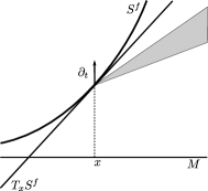
Figure 11. A hypersurface $S^{f}$ in an $\rm SSTK$ splitting $L=\mathds{R}\times M$ satisfying condition (42). The shaded region represents the future-pointing causal vectors in $T_{(f(x),x)}L$

Now, let $(\mathds{R}\times M,g)$ be an $\rm SSTK$ splitting and fix some $f:M\rightarrow\mathds{R}$ under the hypotheses (41) or (42) of the lemma. Define the spacelike hypersurface $S^{f}$ of $(\mathds{R}\times M,g)$ and denote the new $\rm SSTK$ splitting as $(\mathds{R}\times M,g^{f})$, where

$$g^{f}((\tau,v),(\tau,v))=g((df(v)+\tau,v),(df(v)+\tau,v))$$ (45)

for $(\tau,v)\in\mathds{R}\times TM$.

Convention 6.9.

According to the remark above, $\Sigma^{f}$ will denote the Fermat structure associated with $(\mathds{R}\times M,g^{f})$ when $f$ lies in the case (41) and its reverse Fermat structure (see comment before Corollary 3.16) when $f$ lies in the case (42).

Proposition 6.10.

With the above notation,

1. if $F$ and $F_{l}$ are the conic pseudo-Finsler metrics associated with $\Sigma$, then $F^{f}=F-df$ and $F_{l}^{f}=F_{l}-df$ are the conic pseudo-Finsler metrics associated with $\Sigma^{f}$,

2. $\Sigma^{f}$ has the same geodesics as $\Sigma$ up to parametrization.

Proof.

Observe that $g^{f}((\tau,v),(\tau,v))=g_{0}^{f}(v,v)+2\omega^{f}(v)\tau-\Lambda^{f}\tau^{2}$, where

$$\begin{array}[]{rll}g_{0}^{f}(v,v)&=&g((df(v),v),(df(v),v))=g_{0}(v,v)+2\omega(v)df(v)-\Lambda df(v)^{2},\\ \omega^{f}(v)&=&g((df(v),v),(1,0))=\omega(v)-\Lambda df(v)\end{array}$$ (46)

and $\Lambda^{f}=\Lambda$; in particular, the metric $h$ in (34) remains invariant:

$$\Lambda g_{0}^{f}(v,v)+\omega^{f}(v)^{2}=\Lambda g_{0}(v,v)+\omega(v)^{2}.$$ (47)

$(i)$ When $\Lambda(x)=0$, the equality $F^{f}=F-df$ follows directly from (46) (recall (31)). For the case $\Lambda\not=0$, just notice that the expressions of $F,F_{l}$ in (30), (32) can be rewritten as in the first identity of (33), and use (47).

$(ii)$ By Theorem 6.3, the geodesics of $\Sigma^{f}$ are either geodesics of $F^{f}$, geodesics of $F_{l}^{f}$, lightlike pregeodesics of $\Lambda g_{0}^{f}(v,v)+\omega^{f}(v)^{2}$ (except at isolated points) or constant curves with $\Lambda^{f}(x)=0$ and $d\Lambda^{f}({\rm Ker}\,\omega^{f}_{x})\equiv 0$. In the two last cases, they are pregeodesics of $\Sigma$ by (47) and because $d\Lambda({\rm Ker}\,\omega_{x})\equiv 0$ if and only if $d\Lambda^{f}({\rm Ker}\,\omega^{f}_{x})\equiv 0$ in the points where $\Lambda^{f}(x)(=\Lambda(x))=0$. In the other cases, the length functionals of $F^{f}=F-df$ and $F$ (resp. $F_{l}^{f}$ and $F_{l}$), when defined on the space of $F$-admissible (or equivalently $F^{f}$-admissible) curves connecting two prescribed points, are the same up to a constant. Therefore, both functionals have the same critical points and these critical points are pregeodesics of $(M,\Sigma)$ by Theorem 6.3. ∎

Previous interpretations allow us to refine the conclusions of Proposition 6.6 in the Randers-Kropina case.

Corollary 6.11.

Let $(M,F)$ be a Randers-Kropina metric. If the intersection of any closed forward ball and any closed backward one is compact then there exists a new Randers-Kropina metric $F^{f}$ which is geodesically complete and has the same pregeodesics of $F$.

Proof.

As the associated $\rm SSTK$ splitting $(\mathds{R}\times M,g)$ is globally hyperbolic by part $(ii)$ of Theorem 4.9, there exists a smooth spacelike Cauchy hypersurface $S$ (see [11]). As the integral curves of $\partial_{t}$ are causal, they must intersect $S$ transversely and, so, $S$ can be written as a graph $S^{f}$. By Proposition 6.10, the associated splitting $(\mathds{R}\times M,g^{f})$ has a Fermat structure $\Sigma^{f}$ which must be associated with some Randers-Kropina metric $F^{f}=F-df$, and will have the same pregeodesics as $F$. By part $(iii)$ of Theorem 4.9, $\Sigma^{f}$ is geodesically complete. ∎

Remark 6.12.

In the stationary case $\Lambda>0$, the function $f$ can be explained physically as a (new) synchronization of the “observers” travelling along the integral curves of $\partial_{t}$. In the case $\Lambda\geq 0$, Corollary 6.11 extends [23, Theorem 5.10] valid for Randers manifolds (namely, if $R$ is a Randers metric and the closed symmetrized balls are compact then there exists a function $f$ such that $R-df$ is also Randers, plus complete and with the same pregeodesics as $R$). As suggested in that reference and proved in [68], such a result can be extended from Randers to any Finsler manifold. Anyway, notice that in the case of strong wind an additional difficulty occurs in the proof of Corollary 6.11: as the integral curves of $\partial_{t}$ become spacelike, it is not guaranteed that they will cross the Cauchy hypersurface $S$.

6.3. Precedence relation and solution to Zermelo problem

In [51], the authors introduced a notion of precedence, $\prec$, for a conic pseudo-Finsler metric (see Section 4.1). This can be easily extended to any wind Finslerian structure $(M,\Sigma)$ and, moreover, also a less restrictive relation $\preceq$ appears naturally, so that $\prec$ and $\preceq$ resemble, respectively, the chronological and the causal relations in a Lorentzian manifold. Namely, for any $x,y\in M$, we say that $x\prec y$ (resp. $x\preceq y$) if there exists an $F$-wind (resp. wind) curve connecting $x$ to $y$ (i.e $C^{A}_{x,y}\neq\emptyset$, resp. $C^{\Sigma}_{x,y}\neq\emptyset$). Moreover, for any $x\in M$, the $F$-future (resp. $\Sigma$-future, $F$-past, $\Sigma$-past) of $x$ is the set $I_{\Sigma}^{+}(x)$ (resp. $J_{\Sigma}^{+}(x)$, $I_{\Sigma}^{-}(x)$, $J_{\Sigma}^{-}(x)$) defined as $I_{\Sigma}^{+}(x)=\{y\in M:x\prec y\}$ (resp. $J_{\Sigma}^{+}(x)=\{y\in M:x\preceq y\}\cup\{x\}$, $I_{\Sigma}^{-}(x)=\{y\in M:y\prec x\}$, $J_{\Sigma}^{-}(x)=\{y\in M:y\preceq x\}\cup\{x\}$). The following result summarizes the relations between the above-defined $I^{\pm}_{\Sigma},J^{\pm}_{\Sigma}$, and the corresponding future or past sets for the Lorentzian metrics $g$ in $\mathds{R}\times M$ and $-h$ in $M_{l}$.

Proposition 6.13.

For a wind Riemannian structure with associated $\rm SSTK$ splitting $(\mathds{R}\times M,g)$ and natural projection $\pi:\mathds{R}\times M\rightarrow M$:

$$I^{+}_{\Sigma}(x)=\pi\left(I^{+}(0,x)\right), I^{-}_{\Sigma}(x)=\pi\left(I^{-}(0,x)\right),$$

$$J^{+}_{\Sigma}(x)=\pi\left(J^{+}(0,x)\right), J^{-}_{\Sigma}(x)=\pi\left(J^{-}(0,x)\right),$$

where $x\in M,(0,x)\in\mathds{R}\times M$. In particular, $I^{\pm}_{\Sigma}(x)$ are open subsets.

In the case of strong wind ($M=M_{l}$), $I^{+}_{\Sigma}(x)$ and $I^{-}_{\Sigma}(x)$ coincide, resp., with the chronological future and past of $x$ for the Lorentzian metric $-h$ on $M$ endowed with a natural time-orientation.

Proof.

We shall prove the proposition only for the future sets $I^{+}_{\Sigma}$, being the proof for $I^{-}_{\Sigma}$ completely analogous. Let $y\in I^{+}_{\Sigma}(x)$, $\sigma\in C^{A}_{x,y}$. As $\dot{\sigma}^{\pm}(t)\in A$, then $F\big{(}\dot{\sigma}^{\pm}(t)\big{)}<F_{l}\big{(}\dot{\sigma}^{\pm}(t)\big{)}$ and $y\in B^{+}_{\Sigma}(x,r)$, $r\in(\ell_{F}(\sigma),\ell_{F_{l}}(\sigma))$. Thus, Proposition 5.1 ensures that $(r,y)\in I^{+}(0,x)$. For the converse inclusion, just recall that if $(0,x)\ll(r,y)\in\mathds{R}\times M$ then there exists a future-pointing timelike curve $\gamma(s)=(t(s),\sigma(s))$ between $(0,x)$ and $(r,y)$ with $\dot{\sigma}(s)\neq 0$ for all $s$, see footnote 6. Reparameterizing $\gamma$ with respect to $t$ gives an $F$-wind curve between $x$ and $y$ and $y\in I^{+}_{\Sigma}(x)$.

The proof of the inclusions for $J^{\pm}_{\Sigma}$ are analogous except for a slight difference. In fact, for the inclusion $\pi\left(J^{+}(0,x)\right)\subset J^{+}_{\Sigma}(x)$, observe that if $(0,x)<(r,y)$, the existence of a causal curve between $(0,x)$ and $(r,y)$, such that $\dot{\sigma}(s)\neq 0$ for all $s$, is guaranteed except when $x=y$ and $\gamma$ is a lightlike pregeodesic, but in that case $y\in J^{+}_{\Sigma}(x)$, by definition. For the last assertion, recall Proposition 3.20. ∎

Example 6.14.

Even though $\pi:\mathds{R}\times M\rightarrow M$ is an open map (in agreement with the fact that $I^{\pm}_{\Sigma}(x)$ must be open as so is $I^{\pm}(0,x)$) if, say, $J^{+}(0,x)$ is closed, then $J^{+}_{\Sigma}(x)$ is not necessarily closed. Typically, this happens for “black hole regions” (recall Section 8.3) even in globally hyperbolic $\rm SSTK$ splittings. Namely, the causal future of a point $(0,x)$ inside the black hole is closed (as the spacetime is globally hyperbolic) but its causal future may approach the horizon and never touch it. So, the projection $J^{+}_{\Sigma}(x)$ of $J^{+}(0,x)$ admits as boundary points the projection of points of the horizon, but these points do not belong to $J^{+}_{\Sigma}(x_{0})$.

One could define the $F$-separation $d_{F}$ in an analogous way as in the Randers-Kropina case, by using the infimum of the lengths of the $F$-admissible (or $\Sigma$-admissible) curves connecting each two points, as well as a Lorentzian separation $d^{F_{l}}$ by taking the supremum of the $F_{l}$-lengths. In fact, if $F$-admissible curves are taken, then $d_{F}$ lies again in the case of the $F$-separation defined for any conic Finsler structure in [51]. However, as a difference with the Randers-Kropina case, now discontinuities of $d_{F}$ may appear in non-trivial cases. Even though some properties can be proven in this case by using a kind of extended Finsler separation (see Section 9.2), we will ensure directly the existence of geodesics and their extremizing properties by using the previously introduced notions.

Theorem 6.15.

Let $(M,\Sigma)$ be a w-convex wind Riemannian structure and let $x_{0},y_{0}\in M$ such that $y_{0}\in J_{\Sigma}^{+}(x_{0})\setminus{\{x_{0}\}}$. Then:

1. There exists a global minimum $\sigma$ on $C^{\Sigma}_{x_{0},y_{0}}$ of the length functional $\ell_{F}$ which is a pregeodesic of $(M,\Sigma)$, and, when $y_{0}\not\in I_{\Sigma}^{+}(x_{0})$, it is a lightlike pregeodesic of the Lorentzian metric $-h$ in (34), up to isolated points where its derivative vanishes.

2. If $R(x_{0},y_{0}):=\sup\{r>0:y_{0}\in\hat{B}_{\Sigma}^{+}(x_{0},r)\}<+\infty$, there exists a global maximum $\sigma$ on $C^{\Sigma}_{x_{0},y_{0}}$ of the length functional $\ell_{F_{l}}$ which is a pregeodesic of $(M,\Sigma)$, and, when $y_{0}\not\in I_{\Sigma}^{+}(x_{0})$, it is a lightlike pregeodesic of the Lorentzian metric $-h$ (with non-vanishing derivative).

Proof.

$(i)$ Consider the associated $\rm SSTK$ splitting $(\mathds{R}\times M,g)$ and recall that w-convexity implies its causal simplicity (see Theorem 5.9). Given $x_{0},y_{0}$ as above, denote $r(x_{0},y_{0}):=\inf\{r>0:y_{0}\in\hat{B}_{\Sigma}^{+}(x_{0},r)\}$; notice that $0<r(x_{0},y_{0})<+\infty$ (the first inequality follows from Proposition 5.1 and the acausality of $S_{0}$, the second one trivially follows from $y_{0}\in J^{+}_{\Sigma}(x_{0})$). The definition of $r(x_{0},y_{0})$ and Proposition 5.1 imply that $(r_{n},y_{0})\in J^{+}(0,x_{0})$ for some sequence $r_{n}\rightarrow r(x_{0},y_{0})$ with $r_{n}\geq r(x_{0},y_{0})$ and, moreover, $(r^{\prime},y_{0})\not\in J^{+}(0,x_{0})$ if $r^{\prime}<r(x_{0},y_{0})$. So, $(r(x_{0},y_{0}),y_{0})$ lies in the boundary of $J^{+}(0,x_{0})$ and causal simplicity implies that this boundary is contained in $J^{+}(0,x_{0})$. Thus, $(0,x_{0})$ and $(r(x_{0},y_{0}),y_{0})$ are horismotically related and any connecting causal curve from $(0,x_{0})$ to $(r(x_{0},y_{0}),y_{0})$ must be a lightlike pregeodesic. The projection $\sigma$ on $M$ of such a pregeodesic is an extremizing pregeodesic of $(M,\Sigma)$ (recall Corollary 5.3); moreover, $\sigma$ must be a global minimum of $\ell_{F}$ on $C^{\Sigma}_{x_{0},y_{0}}$ otherwise a curve $\sigma_{1}\in C^{\Sigma}_{x_{0},y_{0}}$ should exist such that $\ell_{F}(\sigma_{1})<\ell_{F}(\sigma)=r(x_{0},y_{0})$. As $\ell_{F}(\sigma_{1})\leq\ell_{F_{l}}(\sigma_{1})$, $y_{0}\in\hat{B}_{\Sigma}^{+}(x_{0},\ell_{F}(\sigma_{1}))$ in contradiction with the definition of $r(x_{0},y_{0})$. In the case $y_{0}\not\in I_{\Sigma}^{+}(x_{0})$, the velocity of any connecting $\Sigma$-admissible curve must lie in $A_{E}\setminus A$ at some point and, thus, $\sigma$ must belong to case (ii)-(c) of Theorem 6.3 that implies the last conclusion.

$(ii)$ Notice that the additional hypothesis $R(x_{0},y_{0})<+\infty$ allows us to use the same technique as in the previous part in order to obtain a maximizing pregeodesic $\sigma$ of $(M,\Sigma)$. However, now the velocity of $\sigma$ cannot vanish at some (isolated) point because, in this case, $K$ would be lightlike at that point and one could concatenate an arbitrary segment of integral curve of $K$ at that point. Thus, $R(x_{0},y_{0})=+\infty$, a contradiction. ∎

Example 6.16.

Let us observe that if $y_{0}\in I^{+}_{\Sigma}(x_{0})$ in the part $(i)$ of last theorem, this does not necessarily imply that the solution is a pregeodesic of $F$. This can happen for example in an $\rm SSTK$ whose associated $-h$ is Lorentzian and the slice is compact, as $(\mathds{R}\times T^{2},g)$ with $g=dt^{2}+dx^{2}+dy^{2}-\sqrt{2}(dxdt+dtdx)$ (we consider the torus $T^{2}$ as the quotient of $\mathds{R}^{2}$ with the identifications $(x,y)\sim(x+1,y)$ and $(x,y)\sim(x,y+1)$). In this case, $h=dx^{2}-dy^{2}$ and $(T^{2},-h)$ is totally vicious, so we have that $y_{0}\in I^{+}_{\Sigma}(x_{0})$ for all $x_{0},y_{0}\in T^{2}$. But the spacetime $(\mathds{R}\times T^{2},g)$ is globally hyperbolic and there always exists solution to the associated Zermelo problem, given by a boundary geodesic in some cases as when we consider $x_{0}=(0,0)\in T^{2}$ and $y_{0}=(s,s)\in T^{2}$, for small $s>0$.

From Proposition 6.6-$(ii)$, we have that w-convexity is satisfied if $M$ is compact, and then we get immediately:

Corollary 6.17.

Let $\Sigma$ be the wind Riemannian structure determined by a compact Riemannian manifold $(M,g_{R})$ and a vector field $W$ on $M$. Then for any couple of points $x_{0},y_{0}\in M$, $x_{0}\neq y_{0}$, there exists a curve in $C^{\Sigma}_{x_{0},y_{0}}$ which is a minimum of $\ell_{F}$ provided that at least a wind curve from $x_{0}$ to $y_{0}$ exists.

Theorem 6.15 gives the last step in the solution to Zermelo’s navigation theorem under any type of (time-independent) wind $W$ in a Riemannian background $(M,g_{R})$. As far as we know, the description of this problem as a Finslerian geodesic connectedness problem appeared first in [82], under the assumption that the wind is mild (apart from its time-independence). The case of a wind which is everywhere critical was considered in [89]. Because of its importance, we summarize and discuss the general solution now.

Corollary 6.18 (Summary of the solution to Zermelo’s problem).

Let $\Sigma$ be the wind Riemannian structure determined by a Riemannian manifold $(M,g_{R})$ and a vector field $W$ on $M$ and let $x_{0}\neq y_{0}\in M$:

1. If there exists a solution $\sigma$ to Zermelo navigation connecting $x_{0}$ to $y_{0}$, that is, a regular wind curve from $x_{0}$ to $y_{0}$ which is a global minimum of the length functional $\ell_{F}$ on $C^{\Sigma}_{x_{0},y_{0}}$, then $x_{0}\preceq y_{0}$ and $\sigma$ is a pregeodesic of $(M,\Sigma)$.

   Moreover, $\sigma$ is either a pregeodesic for the conic Finsler metric $F$ (and, thus, $x_{0}\prec y_{0}$), or a lightlike pregeodesic of the Lorentzian metric $-h$ in (34), up to isolated points where its derivative vanishes.

2. If $x_{0}\preceq y_{0}$ and the wind Finslerian structure is w-convex, then there exists a solution to Zermelo navigation from $x_{0}$ to $y_{0}$.

Proof.

Recall that, by Definition 2.20–(iii), $\sigma$ is a piecewise smooth, $\Sigma$-admissible curve whose left and right derivatives can vanish only at a finite number of instants $\sigma(s_{j})$ (being also $0_{\sigma(s_{j})}\in\Sigma_{\sigma(s_{j})}$ and, by Convention 2.19, $F(0_{\sigma(s_{j})}=1$). Since $\ell_{F}(\sigma)<+\infty$, we can assume that $\sigma$ is reparametrized by using its $F$-length. Then, $\sigma$ must be a unit extremizing $\Sigma$-geodesic (according to Definition 2.35) because, otherwise, there would be a connecting wind curve of strictly smaller length. So, the result follows from the classification of $\Sigma$-geodesics in Theorem 6.3. For (ii), just use Theorem 6.15–(i). ∎

In order to apply these results in a practical way, the following comments are in order (see also Figure 10):

1. An obvious necessary condition for the existence of a Zermelo solution between $x_{0},y_{0}$ $(x_{0}\neq y_{0})$ is the possibility to travel from the first to the second point, that is, $y_{0}\in J^{+}_{\Sigma}(x_{0})$. This is a vacuous condition when the wind is mild. When the wind is strong (on all $M$), the question is reduced to study the causal future of $x_{0}$ for the Lorentzian metric $-h$; this is a non-trivial but typical computation in spacetimes (see, e.g., Example 6.19 and Proposition 6.23 below). When there are points with critical wind, then the precedence relation must be studied specifically there; moreover, the possibility of travelling between two critical points by moving freely in the region of mild wind must be also taken into account. Even though, in principle, this may be done directly, from the spacetime viewpoint it becomes equivalent to the existence of a future-pointing causal curve connecting $(0,x_{0})$ to $l_{y_{0}}=\mathds{R}\times\{y_{0}\}$).

2. In the case that the trip is possible, the possible solutions to Zermelo’s navigation must be found in the set of geodesics for the conic Finsler metric $F$ and in the set of piecewise smooth lightlike pregeodesics for $-h$ with $C^{1}$ zero velocity at the breaks and non-vanishing second derivative there.

   The possibility of the existence of these last geodesics was pointed out by Caratheodory in [27, §282], who studied a time-independent wind on a plane. Indeed, he mentioned the possibility of the existence of solutions which are limits of maximal and minimal ones and called “anomalous” their possible velocity vector fields. In a more modern language, these solutions are called abnormal extremals (compare, e.g., with [80, p.54-55], where the Zermelo navigation problem on a plane is analysed).

   We have interpreted abnormal extremals in three equivalent ways: (a) boundary geodesics of $(M,\Sigma)$, (b) lightlike pregeodesics (up to a finite number of instants where the velocity vanishes) of $-h$, and (c) projections of certain lightlike geodesics in the associated SSTK spacetime.

   From the spacetime viewpont, all Zermelo solutions are projections of first arriving future-pointing lightlike pregeodesics connecting $(0,x_{0})$ to $l_{y_{0}}=\mathds{R}\times\{y_{0}\}$.

3. For the existence of maximizing geodesics, assuming the obvious necessary condition $R(x_{0},y_{0})<+\infty$ (apart from $y_{0}\in J^{+}_{\Sigma}(x_{0})$), the possible maximizing curves must be found in the set of geodesics for the Lorentz-Finsler metric $F_{l}$ and in the set of (smooth) lightlike pregeodesics of $-h$.

   Notice that the maximizing geodesics, if they exist, must be entirely contained in the region of strong wind: otherwise, when one crosses a point of non-strong wind, one can concatenate a wind curve segment so that the curve remains close to this point along an arbitrarily long time, before arriving at $y_{0}$.

   From the spacetime viewpoint, all maximizing curves are projections of last arriving future-pointing lightlike pregeodesics connecting $(0,x_{0})$ to $l_{y_{0}}=\mathds{R}\times\{y_{0}\}$.

4. In order to ensure the existence of extremals, the condition of w-convexity becomes the natural one: (a) it holds when $\Sigma$ is complete or any of the conditions in parts $(i)$ and $(ii)$ of Proposition 6.6 holds, (b) it generalizes the classical notion of convexity for domains of Riemannian and Finslerian manifolds, and (c) as in these geometries, it is related to the convexity of the boundary of the domain (see Theorem 6.21 below).

   From the spacetime viewpoint, w-convexity becomes equivalent to the causal simplicity of the spacetime, a standard causality condition. As in the previous cases, the interpretation in the SSTK has a double interest: (i) it may be easier to check, and (ii) it provides the arrival times of the extremal geodesics (namely, the $t$-coordinate at boundary points in $l_{y_{0}}$ of $J^{+}(0,x_{0})\cap l_{y_{0}}$).

5. As in Riemannian Geometry, one can wonder at what extent all the $\Sigma$-pregeodesics from $x_{0}$ to $y_{0}$ are critical points for some length functional. The answer to this question (Theorem 7.8) is postponed to the study of a new general Fermat’s principle for spacetimes and its adaptation for SSTK spacetimes in Section 7.

Example 6.19.

The obvious connectivity condition $y_{0}\in J_{\Sigma}^{+}(x_{0})\setminus{\{x_{0}\}}$ in Zermelo’s problem may fail even if $M$ is compact. Indeed, consider a sphere $S^{2}$ with the natural metric induced by the Euclidean one and a smooth vector field which is given in spherical coordinates $(\theta,\phi)$ by

$$W(\phi,\theta)=\begin{cases}0&\theta\in[0,\pi/6]\cup[\pi/2,\pi]\\ f(\theta)e_{\theta}&\theta\in(\pi/6,\pi/2)\end{cases}$$

where $e_{\theta}$ is the unit vector field associated with the latitude coordinate $\theta$ and the function $f\colon[\pi/6,\pi/2]\to[0,+\infty)$ is smooth, non-negative, equal to $0$ at $\theta=\pi/6,\pi/2$, strictly increasing in $[\pi/6,\pi/4]$, strictly decreasing otherwise and such that $f(\pi/4)>1$. Any wind curve from each point $x_{0}$ in the hemisphere containing the south pole cannot connect points in the open region containing the north pole and having as boundary the parallel of latitude $\bar{\theta}$, where $\bar{\theta}\in(\pi/4,\pi/2)$ is equal to $f^{-1}(1)$. In fact, along the line $p_{\theta}=\{(\phi,\theta):\theta=\bar{\theta}\}$, the set of admissible velocities for wind curves is included in the tangent half-space containing $e_{\theta}$ plus the zero vectors and therefore any wind curve starting on the region $\Omega_{S}=\{(\phi,\theta):\theta>\bar{\theta}\}$ must turn back into $\Omega_{S}$ when arriving to a point on $p_{\theta}$ (compare with Proposition 6.23 below).

6.4. Further results on existence of geodesics

Our methods can also be applied to find a solution of Zermelo navigation problem in quite a few interesting cases. Let us start considering an open subset of a wind Riemannian manifold $(M,\Sigma)$ whose boundary satisfies a convexity assumption. We recall first some notions and results about convexity of the boundary of an open subset which have been studied in [7]. Let $D$ be an open subset of a Finsler manifold $(M,F)$ with smooth boundary. We say that $D$ has locally convex boundary if for each $x\in\partial D$ there exists some neighborhood of $0$ in $T_{x}\partial D$ whose images by both the exponential maps of $F$ and of its reverse Finsler metric $\tilde{F}(v):=F(-v)$ do not intersect $D$. This condition is equivalent to the infinitesimal convexity of $\partial D$ (related to its normal curvature at any point $x\in\partial D$) and will be referred here just as the (extrinsic) convexity of $\partial D$. If $\partial D$ is convex and $x\in\partial D$ then, [7, Lemma 3.5], there exists a small enough convex ball (of the metric $F$) $B^{+}(x,\delta)$ such that for each $x_{1},x_{2}\in D\cap B^{+}(x,\delta)$ the (unique) geodesic in $B^{+}(x,\delta)$ which connects $x_{1}$ with $x_{2}$ is included in $D$. The following lemma is a refinement of that result.

Lemma 6.20.

Let $D$ be an open subset of a Finsler manifold $(M,F)$ with smooth, convex boundary and $x\in\partial D$. Then for all $x_{1},x_{2}\in\bar{D}\cap B^{+}(x,\delta)$, $\delta>0$ small enough, the (unique) geodesic in $B^{+}(x,\delta)$ which connects $x_{1}$ with $x_{2}$ is included in $\bar{D}$. In particular, if $x_{1},x_{2}\in\partial D$ then it is either contained in $\partial D\cap B^{+}(x,\delta)$ or it is contained in $D\cap B^{+}(x,\delta)$, except for its endpoints, and it is not tangent to $\partial D$ in the endpoints. This last case always happens if at least one of the points $x_{1}$, $x_{2}$ belongs to $D$.

Proof.

Choosing $\delta$ as in the discussion above, only the case when at least one of the points $x_{1},x_{2}$ belongs to $\partial D$ must be taken into account. Take two sequences of points $\{x^{1}_{k}\},\ \{x^{2}_{k}\}\subset D\cap B^{+}(x,\delta)$ converging resp. to $x_{1}$ and $x_{2}$. Consider the geodesics $\gamma_{k}$ connecting $x^{1}_{k}$ with $x_{k}^{2}$ which are contained in $D\cap B^{+}(x,\delta)$, [7, Lemma 3.5]. By smooth dependence of geodesics in a convex neighborhood from endpoints, $\gamma_{k}$ converges (in the $C^{2}$-topology) to the geodesic $\gamma$ connecting $x_{1}$ and $x_{2}$ in $B^{+}(x,\delta)$. Thus, $\gamma$ is contained in $\bar{D}$ and it is tangent to $\partial D$ when it touches the boundary away from the endpoints. By the definition of local convexity, this easily implies that $\gamma$ is either contained in the boundary or it touches the boundary transversally at most in the endpoints. ∎

By using the above lemma and the correspondence between $\rm SSTK$ spacetimes and wind Riemannian structures, we can prove the existence of a solution to Zermelo navigation problem in an open subset $D\subset M$ such that $\partial D$ is compact. To this end, we need to consider wind curves whose image is contained in $\bar{D}$ and we will recall this by using the symbol $\Sigma|_{\bar{D}}$. For example, given $x_{0},y_{0}\in\bar{D}$, $C^{\Sigma|_{\bar{D}}}_{x_{0},y_{0}}$ denotes the subset of wind curves from $x_{0}$ to $y_{0}$ with image in $\bar{D}$.

Theorem 6.21.

Let $(M,\Sigma)$ be a wind Riemannian structure, $D\subset M$ be a precompact, open subset with smooth boundary $\partial D$, and let $x_{0},y_{0}\in\bar{D}$ such that $y_{0}\in J_{\Sigma|_{\bar{D}}}^{+}(x_{0})\setminus{\{x_{0}\}}$. Assume that the wind is mild on $\partial D$ and that this boundary is convex for $F$. Then there exists a global minimum $\sigma$ on $C^{\Sigma|_{\bar{D}}}_{x_{0},y_{0}}$ of the length functional $\ell_{F}$ and it fulfils one of the following two possibilities:

1. $\sigma$ is fully contained in $\partial D$ and, thus, it is a geodesic of both, $F$ and the Finsler metric induced by $F$ on $\partial D$;

2. $\sigma$ is contained in $D$ except, at most, its endpoints.

In particular, this last case happens when one of the points $x_{0}$, $y_{0}$ belongs to $D$. Moreover if (b) occurs: (i) $\sigma$ is a pregeodesic of $(M,\Sigma)$ and (ii) when $y_{0}\not\in I_{\Sigma|_{\bar{D}}}^{+}(x_{0})$, then $\sigma$ is also a lightlike pregeodesic of the Lorentzian metric $-h$ in (34), up to isolated points where its derivative vanishes.

Proof.

As $y_{0}\in J_{\Sigma|_{\bar{D}}}^{+}(x_{0})\setminus{\{x_{0}\}}$, the set of wind curves between $x_{0}$ and $y_{0}$ whose image is contained in $\bar{D}$ is not empty. We want to find a curve $\sigma\in C^{\Sigma|_{\bar{D}}}_{x_{0},y_{0}}$ which attains the infimum

$$T_{0}(x_{0},y_{0}):=\inf_{\sigma\in C^{\Sigma|_{\bar{D}}}_{x_{0},y_{0}}}\ell_{F}(\sigma).$$

Consider an $\rm SSTK$ spacetime $(\mathds{R}\times M,g)$ associated with $(M,\Sigma)$ (see part $(i)$ of Theorem 3.10) and the subset of curves

$$C^{cc|_{\bar{D}}}_{x_{0},y_{0}}=\{\gamma:[a_{\gamma},b_{\gamma}]\rightarrow\mathds{R}\times\bar{D}\subset\mathds{R}\times M:\text{$\gamma$ future-pointing causal continuous,}\\ \quad\quad\quad\quad\quad\quad\gamma(a_{\gamma})=(0,x_{0}),\ \pi\big{(}\gamma(b_{\gamma})\big{)}=y_{0},\ a_{\gamma}<b_{\gamma}\}$$

(recall Definition 4.4 and the paragraph below it for the notion of causal continuous curve). Now define

$$T_{1}(x_{0},y_{0}):=\inf_{\gamma\in C^{cc|_{\bar{D}}}_{x_{0},y_{0}}}T(\gamma),$$

where $T(\gamma)$ is the arrival time, namely, the first coordinate of $\gamma(b)$. Observe that $T_{1}(x_{0},y_{0})\leq T_{0}(x_{0},y_{0})$, since each curve in $C^{\Sigma|_{\bar{D}}}_{x_{0},y_{0}}$ can be lifted to a future-pointing lightlike curve $\gamma(t)=(t,\sigma(t))$ such that $\ell_{F}(\sigma)=T(\gamma)$ (see the proof of Proposition 5.1). It is enough to prove that the infimum $T_{1}(x_{0},y_{0})$ is attained by a future-pointing lightlike pregeodesic which, by Theorem 5.5, projects into a pregeodesic $\sigma$ of $(M,\Sigma)$ with $\ell_{F}(\sigma)=T_{1}(x_{0},y_{0})\leq T_{0}(x_{0},y_{0})$. Take a sequence of curves $\{\gamma_{k}\}$ in $C^{cc|_{\bar{D}}}_{x_{0},y_{0}}$ such that $\lim_{k}T(\gamma_{k})=T_{1}(x_{0},y_{0})$, which can be assumed parametrized by the first coordinate, namely, $\gamma_{k}(t)=(t,\sigma_{k}(t))$. Then by Lemma 5.7, there exists a limit curve $\gamma(t)=(t,\sigma(t))$ defined on $[0,T_{1}(x_{0},y_{0})]$ which is future-pointing causal continuous. Let us see that $\gamma$ is a future-pointing lightlike geodesic:

Case (i): let us first consider an instant $t_{0}\in(0,T_{1}(x_{0},y_{0}))$ such that $\sigma(t_{0})\in D$. Then there exists $\varepsilon>0$ such that $\gamma([t_{0}-\varepsilon,t_{0}+\varepsilon])\subset D$. Moreover, if $\gamma|_{[t_{0}-\varepsilon,t_{0}+\varepsilon]}$ is not a future-pointing lightlike pregeodesic, there exists a smooth causal curve $\beta$ from $\gamma(t_{0}-\varepsilon)$ to $(t_{0}+\varepsilon-\epsilon,\sigma(t_{0}+\varepsilon))$ for some $\epsilon>0$. In order to prove the existence of $\beta$ recall that by definition of causal continuous curve we can find a piecewise smooth causal curve close to $\gamma|_{[t_{0}-\varepsilon,t_{0}+\varepsilon]}$. Then by [72, Proposition 10.46], if it is not a future-pointing lightlike pregeodesic, we can find a future-pointing timelike curve from $\gamma(t_{0}-\varepsilon)$ to $\gamma(t_{0}+\varepsilon)$ and the conclusion follows using that the chronological relation is open. Now consider the concatenation $\tilde{\gamma}=\gamma|_{[0,t_{0}-\varepsilon]}\ast\beta\ast\bar{\gamma}$, where $\bar{\gamma}(t)=(t-\epsilon,\sigma(t))$ is defined in $[t_{0}+\varepsilon,T_{1}(x_{0},y_{0})]$. It turns out that $T(\tilde{\gamma})=T_{1}(x_{0},y_{0})-\epsilon$, a contradiction.

Case (ii): assume now that $\gamma(t_{0})\in\partial D$ for $t_{0}\in(0,T_{1}(x_{0},y_{0}))$ and consider a ball $B^{+}(\gamma(t_{0}),\delta)$ as in Lemma 6.20. There exists $\varepsilon>0$ such that $\gamma|_{[t_{0}-\varepsilon,t_{0}+\varepsilon]}$ is contained in $B^{+}(\gamma(t_{0}),\delta)$. Moreover, $\sigma|_{[t_{0}-\varepsilon,t_{0}+\varepsilon]}$ minimizes the $F$-length from $\sigma(t_{0}-\varepsilon)$ to $\sigma(t_{0}+\varepsilon)$, because otherwise if there exists a shorter curve $\tilde{\sigma}$, one can construct a causal continuous curve by concatenation as in case (i), using $\beta(t)=(t,\tilde{\sigma}(t))$ and $\epsilon=\ell_{F}(\sigma)-\ell_{F}(\tilde{\sigma})$. Being $\sigma|_{[t_{0}-\varepsilon,t_{0}+\varepsilon]}$ $F$-minimizing, we conclude by Lemma 6.20 that it is a geodesic contained in $\partial D$.

Case (ii) also implies conditions (a) and (b), and the final statement follows from part (i) of Theorem 6.15.

∎

Remark 6.22.

The last result of convexity can be extended with the same technique to more general cases. For example, when the wind is mild outside a compact subset $K\subset D$, $\partial D$ is convex, and $D\setminus K$ is forward (or backward) complete, in the sense that any $F$-geodesic $\gamma:[0,b)\rightarrow D\setminus K$ which is inextendible to $b$ in $D\setminus K$, either converges to some point in $\partial D\cup K$ or satisfies $b=\infty$. Recall also that another characterizations of this property can be easily obtained from Theorem 2.1 (a),(b) and (e) in [23] (this includes the compactness of the closed forward balls, which makes possible to reduce the non-compact case to the solved one in Theorem 6.21).

Now, let us focus on the case of strong wind. i.e., $M=M_{l}$. In the compact case, the unique condition for the existence of Zermelo solutions is the assumption of precedence, and it is easy to find conditions ensuring it for any two points.

Proposition 6.23.

Let $(M,\Sigma)$ be a wind Riemannian structure with strong wind and compact $M$. If the Lorentzian metric $-h$ is endowed with a timelike conformal Killing vector field then $y_{0}\in I^{\pm}_{\Sigma}(x_{0})$, for any couple of points $x_{0},y_{0}\in M$. Therefore, Zermelo navigation problem has always a solution for any couple of points.

In particular, such a vector field exists if the strong wind data $(g_{R},W)$ satisfy that $W$ is Killing for $g_{R}$.

Proof.

By [79, Th. 1] a compact Lorentzian manifold $M$ with a timelike conformal Killing vector field is totally vicious, i.e. the chronological future and past of every point $x_{0}\in M$ are equal to $M$. Since for a strong wind the chronological relation on $(M,-h)$ coincides with the precedence relation on $(M,\Sigma)$ (recall last part of Proposition 6.13) the result follows (the assertion on Zermelo follows from Theorem 6.15-(i)). For the last assertion, just notice that $W$ must be then also timelike and Killing for $-h$ (use (34) with $g_{R}=g_{0}$, $\Lambda=1-g_{R}(W,W)$ and $\omega=-g_{R}(\cdot,W)$). ∎

For the existence of maximizing geodesics, the (obviously necessary) hypothesis on $R(x_{0},y_{0})$ in Theorem 6.15(ii), never can hold if $y_{0}\not\in M_{l}$. However, the next lemma provides a natural sufficient condition.

Lemma 6.24.

Let $x_{0},y_{0}\in M$ and assume that there exists $\bar{r}>0$ such that $y_{0}\in\hat{B}_{\Sigma}^{+}(x_{0},\bar{r})$. Then $R(x_{0},y_{0})<+\infty$ whenever (i) the wind is strong (i.e. $M=M_{l}$), and (ii) the metric $-h$ is globally hyperbolic.

Proof.

As global hyperbolicity is preserved by conformal changes, $(M,\frac{1}{\Lambda}h)$ and $(M,-\frac{1}{\Lambda^{2}}h)$ are also globally hyperbolic (recall that $\Lambda<0$ if $M=M_{l}$). Since $y_{0}\in\hat{B}^{+}_{\Sigma}(x_{0},\bar{r})$, $x_{0}$ and $y_{0}$ are causally related in $(M,-h)$. Thus, by global hyperbolicity, the length w.r.t. the Lorentzian metric $-\frac{1}{\Lambda^{2}}h$ of all the future-pointing $-h$-causal curves between them is bounded (see [8, Lemma 4.5]). Moreover, since they are causal curves, the length w.r.t. the Riemannian metric $-\frac{1}{\Lambda}g_{0}$ is bounded as well (see [8, p. 76]). As, $\frac{1}{\Lambda^{2}}\omega(v)^{2}=\frac{1}{\Lambda^{2}}h(v,v)-\frac{1}{\Lambda}g_{0}(v,v)$, then

$$\big{|}\frac{1}{\Lambda}\omega(v)\big{|}\leq\sqrt{\frac{1}{\Lambda^{2}}h(v,v)}+\sqrt{-\frac{1}{\Lambda}g_{0}(v,v)}$$

for every causal $v\in TM$, which implies that the $F_{l}$-length of all the $\Sigma$-admissible curves between those two points is bounded (recall that $F_{l}=\sqrt{h/\Lambda^{2}}+\omega/\Lambda$, Fig. 6) and consequently $R(x_{0},y_{0})<+\infty$. ∎

Example 6.25.

The global hyperbolicity of $-h$ is not implied by the global hyperbolicity of the $\rm SSTK$ splitting: a counterexample is any $\rm SSTK$ splitting with compact slices such that $K$ is spacelike; indeed, the SSTK spacetime is globally hyperbolic (apply part $(iii)$ of Theorem 5.9), but $-h$ can never be globally hyperbolic (as compactness implies that it admits closed timelike curves, i.e., $-h$ is not chronological). An explicit counterexample is the Lorentzian cylinder $\mathds{R}\times S^{1}$, $g=dt^{2}-4dtd\theta+d\theta^{2}$. However, the next lemma shows that the converse holds.

Lemma 6.26.

In the case of strong wind, if $-h$ is globally hyperbolic then the associated $\rm SSTK$ splitting is also globally hyperbolic.

Proof.

Since $\pi:(\mathds{R}\times M,g)\rightarrow(M,\frac{1}{\Lambda}h)$ is a Lorentzian submersion, one can easily check that a lift of any Cauchy hypersurface on $(M,\frac{1}{\Lambda}h)$ is also a Cauchy hypersurface of $(\mathds{R}\times M,g)$. ∎

The previous lemmas yield a nice result on the existence of maximizing geodesics.

Theorem 6.27.

Let $(M,\Sigma)$ be a wind Riemannian structure with strong wind such that the Lorentzian metric $-h$ is globally hyperbolic. For any $x_{0}\in M$, if $y_{0}\in J_{\Sigma}^{+}(x_{0})\setminus\{x_{0}\}$ then there exists a global maximum on $C^{\Sigma}_{x_{0},y_{0}}$ of the length functional $\ell_{F_{l}}$.

Proof.

Apply Theorem 6.15 by taking into account that Lemma 6.26 ensures w-convexity and Lemma 6.24 ensures that the hypothesis in the last part of that theorem is fulfilled. ∎

Finally, let us give an application to the existence of closed geodesics. The differences between the causal properties of the Lorentzian metric $-h$ on all the manifold $M$, and the metric $g$ of the associated $\rm SSTK$ splitting, were stressed in Example 6.25. They are exploited now to prove the following result.

Theorem 6.28.

Let $(M,\Sigma)$ be a wind Riemannian structure with strong wind. If $M$ is compact then $(M,\Sigma)$ admits a closed (non-constant) geodesic.

Proof.

Consider the associated $\rm SSTK$ splitting and define:

$$T_{0}=\inf_{x\in M}\{T_{0}(x)\}\qquad\hbox{where}\qquad T_{0}(x)=\inf\{T>0:(0,x)\ll(T,x)\}.$$

Notice that $T_{0}<+\infty$. In fact, any closed timelike curve $\sigma:[0,1]\rightarrow M$ for $-h$ provides an $\rm SSTK$-timelike curve $\tilde{\sigma}(s)=(\eta(s),\sigma(s)),s\in[0,1]$, $2\eta(s)=\int_{0}^{s}(F(\dot{\sigma}(\bar{s}))+F_{l}(\dot{\sigma}(\bar{s})))d\bar{s}$ from $(0,\sigma(0))$ to $(T=\eta(1),\sigma(0))$, so that $T_{0}(\sigma(0))<+\infty$. Notice also that, as the associated $\rm SSTK$ splitting is strongly causal, $T_{0}(x)>0$ for each $x\in M$ and, whenever $T_{0}(x)<+\infty$, $(0,x)$ and $(T_{0}(x),x)$ can be joined by a lightlike geodesic $\gamma_{x}$ (since the associated $\rm SSTK$ splitting is globally hyperbolic, $J^{+}(0,x)$ is closed, so $(T_{0}(x),x)\in J^{+}(0,x)\setminus I^{+}(0,x)$). Now, consider a sequence $\{x_{n}\}\subset M$ such that $T_{0}(x_{n})\rightarrow T_{0}$ and, with no loss of generality, assume that $x_{n}\rightarrow x_{0}$. We claim that $T_{0}>0$ (see below). Thus, a limit curve $\gamma_{0}$ (not reduced to a point) of the corresponding sequence of curves $\{\gamma_{x_{n}}\}$ will exist and connect $(0,x_{0})$ to $(T_{0},x_{0})$ (so that $T_{0}=T_{0}(x_{0})$) and it must be a lightlike pregeodesic too. Hence, being $\partial_{t}$ spacelike, its image cannot be $l_{x_{0}}$ and by Theorem 5.5, its projection $\sigma_{0}=\pi\circ\gamma_{0}$ must be a pregeodesic of $(M,\Sigma)$ with endpoints equal to $x_{0}$. In order to check that $\sigma_{0}$ must be closed, assume that $\sigma_{0}$ and $\gamma_{0}$ are parametrized on $[0,1]$, extend $\sigma_{0}$ periodically, and extend $\gamma_{0}$ accordingly by making it invariant under the translation $(t,x)\mapsto(t+T_{0},x)$. If the velocities $\dot{\sigma}_{0}(0),\dot{\sigma}_{0}(1)$ do not match, then the points $x_{-}=\sigma_{0}(1-\varepsilon),x_{+}=\sigma_{0}(\varepsilon)$ on $\sigma_{0}$ for some $0<\varepsilon<1/2$ satisfy, by well known local causality properties of a Lorentzian manifold (applied to $(M,-h)$) $x_{-}\preceq x_{0}\preceq x_{+}$. Accordingly, $\gamma_{0}(1-\varepsilon)\leq\gamma_{0}(1)\leq\gamma_{0}(1+\varepsilon)$. As $\gamma_{0}$ is a lightlike geodesic broken at $\gamma_{0}(1)$, we can modify it into a causal curve $\rho$ by putting a timelike segment from $\gamma_{0}(1-\varepsilon)$ to $\gamma_{0}(1+\varepsilon)$ and making $\rho$ invariant under the translation $(t,x)\mapsto(t+T_{0},x)$ too. Then, there exists a point $\bar{x}\in M$ such that $\rho(0)=(0,\bar{x})$, $\rho(1)=(T_{0},\bar{x})$ and $\rho_{|[0,1]}$ is not a lightlike pregeodesic. Therefore, for $\varepsilon$ small enough $(0,\bar{x})\ll(T_{0}-\varepsilon,\bar{x})$, in contradiction with the definition of $T_{0}$.

Claim: $T_{0}>0$.

Assume, by contradiction, that $T_{0}(x_{n})\rightarrow 0$, $x_{n}\rightarrow x_{0}$, and choose a neighborhood $W_{0}\subset M$ of $x_{0}$ such that $-h$ restricted to $W_{0}$ is causal. By Lemma 6.4, there exists a new neighborhood $U_{0}\subset W_{0}$ and some $\varepsilon>0$ such that any $\Sigma$-admissible closed curve starting at any $y\in U_{0}$ and leaving $W_{0}$ will leave $\hat{B}^{+}_{\Sigma}(y,r)$, for each $r\in[0,\varepsilon)$. Nevertheless, for large $n$ one has $x_{n}\in U_{0}$ and $T_{0}(x_{n})<\varepsilon$. So, the projection $\sigma_{n}$ of the lightlike geodesic $\gamma_{x_{n}}$ will be a $\Sigma$-admissible loop based at $x_{n}$ (thus leaving $W_{0}$) with $F$-length smaller than $\varepsilon$. As $\ell_{F}(\sigma_{n})\leq\ell_{F_{l}}(\sigma_{n})$, each point of $\sigma_{n}$ must belong to $B^{+}_{\Sigma}(x_{n},r)$ for some $r\in[0,\varepsilon)$, a contradiction. ∎

Remark 6.29.

The closed geodesic in Theorem 6.28 corresponds, in the associated $\rm SSTK$ splitting, to a future-pointing, lightlike geodesic which has closed component $x$ and connects the points $(0,x_{0}),(T_{0},x_{0})\in\mathds{R}\times M$, for each $x_{0}$ belonging to the support of $x$ (these geodesics are called $T_{0}$-periodic trajectories in [16, 78, 13]). This extends to the case of a spacelike Killing vector field $K$ (using the only topological assumption that $M$ is compact) results on the existence of at least one geometrically non-trivial, lightlike, $T$-periodic trajectory, when $K$ is timelike, obtained in [16, 66]. Indeed, the proof of Theorem 6.28 is inspired by a well known result by Tipler [84] as well as results on $T$-periodic trajectories in [78] –even though the reader will find quite a few non-trivial differences. Notice that if the wind were not strong at some point (non-spacelike $K$), the previous proof would fail as $T_{0}$ would be equal to $0$. Nevertheless, in the case of mild wind (timelike $K$) a closed (non-constant) geodesic must exist. In fact, this is known for any compact Finsler manifold [60] and, thus, for Randers ones. Whether a closed geodesic must exist when $K$ is allowed to be lightlike at some point may deserve a further study. The case when $K$ is lightlike everywhere has been recently studied in [19].

To end this section, let us digress on some links to other variational problems on curves in the literature and possible prospects.

(1) It is worth to stress that the dynamics of Zermelo’s navigation is not equivalent to the one of a system defined by a Riemannian metric $g_{R}$ and a one-form $\omega$ on a manifold $M$ (a particular case of the so-called magnetic geodesic flow) except, obviously, if $\|\omega\|_{g_{R}}<1$ because in this case both problems are then described by standard Finsler geometry.

(2) Nevertheless, one can find a parallelism between Zermelo navigation problem and the problem of the existence of timelike or causal curves $\rho$ connecting two events $z_{0},w_{0}$ in a spacetime $L$ which are critical for the action functional associated with an electromagnetic field for some prescribed charge-to-mass ratio $q/m$ (so that the timelike critical curves are solutions to the corresponding Euler-Lagrange equation, i.e., the Lorentz force equation for $q/m$, see e.g. [24, 69, 70]). These curves can be interpreted, say, in the case when $q/m>0$, as those lightlike geodesics for a Kaluza-Klein spacetime $L\times\mathds{R}$ which locally minimize the natural arrival coordinate at $\{w_{0}\}\times\mathds{R}$, see [70, Theorem 4.1]. Even though the natural projection $y:L\times\mathds{R}\rightarrow\mathds{R}$ is not a temporal function for the Kaluza Klein metric, the natural vector field $\partial_{y}$ is Killing. The similarities between the $\rm SSTK$ approach for Zermelo navigation and the Kaluza-Klein for electromagnetism suggests the following navigation problem, whose electromagnetic analogous was solved in [70]:

Consider classes of wind curves from $x_{0}$ to $y_{0}$ which are homotopic through $F$- (resp. $\Sigma$-) wind curves, and determine when such a class admits an $F$-length minimizing (or $F_{l}$-length maximizing) curve.

Even though, in principle, our techniques would allow one to ensure the existence of $\Sigma$-wind curves (under background hypotheses such as completeness or $w$-convexity), subtleties would appear for the existence of critical $F$-wind curves when $x_{0}\prec y_{0}$. This problem has a parallelism with the existence of critical points for the electromagnetic action in timelike or causal homotopy classes, where very precise results (which ensure the existence of timelike critical curves, not only lightlike ones) have been obtained, [70, Theorems 4.2 and 5.1]. Although such techniques seem translatable here, they would require the developing of further notions on wind geodesics (such as cut points) and, so, this will not be studied here.

7. Fermat’s principle and generalized Zermelo navigation problem.

7.1. A new problem: Fermat’s principle for arbitrary arrival curves

In optics, Fermat’s principle is a variational principle for light rays. Its formulations in general relativity, as e.g. in [57, 74, 41, 75], involve a prescribed event (a point $p$ on the Lorentzian manifold $L$ modeling the spacetime, which represents the event of light reception), the world-line of a light source (a timelike injective curve $\alpha\colon(a,b)\to L$), intersecting the causal past of $p$, an “arrival time functional” (the proper time in which the light source emitted the light signals). If some matter distribution (one or more galaxies, dark matter, etc., encoded in the spacetime metric $g$) is present between the source and the observer, it can cause the bending of light producing then the so-called gravitational lensing . From a geometric point of view, this configuration is equivalent to the case to be considered here when the light source emits the signals at a given event $p$ and the timelike curve $\alpha$, intersecting the causal future of $p$, is the world line of an observer (so that, the name “arrival time functional” is justified). From the properties of chronological and causal futures, it is easy to check that if there exists a lightlike (or causal) curve where the absolute maximum or minimum arrival time to $\alpha$ is achieved, this curve must be a lightlike pregeodesic. This is a consequence of the fact that the arrival point would be horismotically related to $p$ and this would hold even if $\alpha$ is not timelike. However, Fermat’s principle states that the set of critical points of the arrival time is equal to the set of lightlike pregeodesics connecting $p$ and $\alpha$ and the timelike character of $\alpha$ is required then. As emphasized by V. Perlick, no external notion of time is necessary, but just the arrival instant $\bar{t}$ with respect to the proper time parametrization of $\alpha$.

Nevertheless, in an $\rm SSTK$ splitting, it is natural to consider the temporal function $t$ and then to ask if Fermat’s principle holds when considering a point and an integral line of the Killing field $\partial_{t}$ (we recall that an integral curve $l_{x_{1}}$, $x_{1}\in M$, of $\partial_{t}$ can be parametrized with the temporal function $t$ of the $\rm SSTK$ splitting, so that the arrival time functional makes still sense). We emphasize that $l_{x_{1}}$ can be spacelike or lightlike now (the case when the Killing vector field is timelike is well known, see [39, 21]) and these possibilities have a clear interpretation in Zermelo’s navigation problem since the travel time can be identified, up to an initial constant, with the arrival time functional of the associated $\rm SSTK$ splitting. Indeed, Fermat’s principle can be viewed as a variational principle for a generalized Zermelo’s navigation problem, namely: look not only for the quickest navigation paths but also for any path that makes critical the time of navigation between two given points $x_{0},x_{1}\in M$. These paths will be the projections on $M$ of the paths in $\mathds{R}\times M$ which are critical for the arrival time functional at $l_{x_{1}}$ defined on the set of the piecewise smooth future-pointing lightlike curves connecting $p_{0}=(t_{0},x_{0})$ to $l_{x_{1}}$.

Summing up, a Fermat’s principle in SSTK spacetimes valid for lightlike curves from $p_{0}$ to any (timelike, spacelike or lightlike) $l_{x_{1}}$ would allow an interpretation of all the geodesics of a wind Riemannian structure as critical points for the arrival functional. However, this problem poses a general mathematical question for Fermat’s principle: when one considers the critical lightlike curves starting at a point $p_{0}$ and arriving at a curve $\alpha$ in an arbitrary spacetime, is it necessary to impose a prescribed causal character or any other hypotheses on $\alpha$?

At first glance, two natural restrictions appear: (a) a connecting lightlike curve $\gamma$ that is orthogonal to $\alpha$ at the arrival point $z_{\alpha}$ would not be permitted (otherwise, $\gamma$ could be a lightlike pregeodesic which coincided with $\alpha$ in a left neighborhood of the end-point and, thus, $\gamma$ would not be a critical point) and (b) $\alpha$ must be an embedded curve, that is, on the one hand its velocity must not be zero (in order to avoid bothering requirements on the variations); on the other, self-intersections or cases where the induced topology on the image is coarser than the one coming from an immersion should be excluded (in order to define properly the Fermat functional as the value of the parameter of $\alpha$ at the arrival point). Recall that these conditions are assumed in previous results, in fact, the requirements (a) and (b), the latter at least locally, hold classically as $\alpha$ is assumed to be a timelike curve; nevertheless in all the proofs we are aware of, the timelike character of $\alpha$ appears to be a fundamental assumption (compare [85, Lemma 2.5], [74, Lemma 3], [3, Lemma 2.1], [41, Remark 3.3]).

In the next subsection we will check that, amazingly, these two conditions are enough for a consistent general Fermat’s principle in spacetimes (Theorem 7.4). Moreover, in the last subsection we will prove that the particular structure of $\rm SSTK$ spacetimes makes unnecessary assumption (a) when $\alpha$ is a line $l_{x_{1}}(\not\ni p_{0})$, (of course, in this case, (b) is satisfied) and, even more, sharper conclusions can be obtained (Theorem 7.8).

7.2. A general Fermat’s Principle

Our aim is to establish a Fermat’s principle between a point $p_{0}$ and an arbitrary smooth embedded curve $\alpha$ for an arbitrary spacetime $(L,g)$.

Given a vector field $\xi=\xi(s)$ along a curve $\gamma$, we will denote by $\xi^{\prime}$ its covariant derivative $\frac{D\xi}{ds}$ with respect to the Levi-Civita connection of $g$. Let us introduce the variational approach for Fermat’s principle.

Definition 7.1.

Let $(L,g)$ be any spacetime, $\alpha:(\bar{a},\bar{b})\rightarrow L$ a smooth embedded curve in $L$, $p_{0}\in L$. Fix an interval $[a,b]$ (eventually normalized to $[0,1]$), and put

$$\mathcal{N}_{p_{0},\alpha}=\{\gamma:[a,b]\rightarrow L:\text{ $\gamma$ piecewise smooth, future-pointing lightlike,}\\ \text{ and $\gamma(a)=p_{0},\ \gamma(b)\in{\rm Im}(\alpha)$}\}$$ (48)

(i) The arrival functional $T:\mathcal{N}_{p_{0},\alpha}\rightarrow\mathds{R}$ is defined as

$$T(\gamma)=\alpha^{-1}(\gamma(b))$$ (49)

(ii) An admissible variation $\chi$ of $\gamma\in\mathcal{N}_{p_{0},\alpha}$ is a $C^{1}$ map $\chi\colon(-\varepsilon,\varepsilon)\times[a,b]\to L$ which has, at least, continuous second order mixed derivatives $\frac{\partial^{2}\chi}{\partial w\partial s},\ \frac{\partial^{2}\chi}{\partial s\partial w}$ on $(-\varepsilon,\varepsilon)\times[s_{j},s_{j+1}]$ (so that, there, $\frac{D}{dw}\frac{\partial\chi}{\partial s}=\frac{D}{ds}\frac{\partial\chi}{\partial w}$), where $a=s_{1}<s_{2}<\ldots<s_{n}=b$ is a subdivision of the interval $[a,b]$, and such that $\gamma_{w}:=\chi_{w}=\chi(w,\cdot)\in\mathcal{N}_{p_{0},\alpha}$, for all $w\in(-\varepsilon,\varepsilon)$, and $\chi_{0}=\gamma$. The variational vector field $Z$ associated with an admissible variation is $Z(s)=\frac{\partial\chi}{\partial w}(0,s)$.

(iii) A curve $z\in\mathcal{N}_{p_{0},\alpha}$ is a critical point of the arrival functional if, for every variation $\gamma_{w}$, we have that $\frac{\mathrm{d}}{\mathrm{d}w}T(\gamma_{w})|_{w=0}=0$.

A basic fact in the proof of the next Lemma is that any $m$-dimensional spacetime can be locally described as a product manifold $(c,d)\times\Omega$, where $\Omega$ is an open, $m-1$ dimensional, smooth manifold endowed with the metric

$$g((\tau,v),(\tau,v))=-\Lambda^{t}(x)\tau^{2}+2\omega^{t}(v)\tau+g_{0}^{t}(v,v)$$ (50)

where $(\tau,v)\in T_{(t,x)}((c,d)\times\Omega)\equiv\mathds{R}\times T_{x}\Omega$ and for every $t\in(c,d)$, $\Lambda^{t}$, $\omega^{t}$ and $g^{t}$ are respectively a function, a one-form and a Riemannian metric in $\Omega$ (under the analogous to (27)). Observe that the coordinate $t\in(c,d)$ also determines a temporal function of $((c,d)\times\Omega,g)$ as for an $\rm SSTK$ spacetime. Thus, this time-orientation and a notation consistent with the previously introduced one for the $\rm SSTK$ case will be used; for example, the line $l_{x_{1}}=\{(s,x_{1}):s\in(c,d)\}$ for every $x_{1}\in\Omega$. In particular, a vector field $Z$ along a curve $\gamma$ with image in $(c,d)\times\Omega$ will be denoted by $Z(s)=(Y(s),W(s))$.

Lemma 7.2.

Let $(L,g)$ be a spacetime, $p_{0}\in L$ and $\alpha:(\bar{a},\bar{b})\rightarrow L$ be any smooth, embedded curve in $L$. Assume that $\gamma:[a,b]\rightarrow L$ is a piecewise smooth future-pointing lightlike curve from $p_{0}$ to ${\rm Im}(\alpha)$, such that $\dot{\gamma}(b)$ is not orthogonal to $\dot{\alpha}(T(\gamma))$. Then there exists a partition $s_{0}=a<s_{1}<\ldots<s_{n}=b$ of the interval $[a,b]$ and $n$ open subsets $U_{1},U_{2},\ldots,U_{n}\subset L$ such that $\gamma$ is smooth in $[s_{j},s_{j+1}]$ with $\gamma([s_{j},s_{j+1}])\subset U_{i+1}$ for $i=0,\ldots,n-1$. Moreover, each $U_{j}$ is of the type $(-\varepsilon_{j},\varepsilon_{j})\times\Omega_{j}$ and the metric $g$ is written as in (50) with $\partial_{t}$ nowhere orthogonal to $\gamma$, and $\alpha$ an integral curve for $\partial_{t}$ or $-\partial_{t}$ in $U_{n}$.

Proof.

As a first step, recall that there exists a vector field $X$ defined on all $M$ such that $X$ is not orthogonal (thus, neither tangent) to $\gamma$ at any point and $\alpha$ is the integral curve of $X$ on a neighborhood $W$ of $q=\gamma(b)=\alpha(T(\gamma))$. Indeed, take any future-pointing timelike vector field $X_{1}$ on $M$, which is necessarily non-orthogonal to $\dot{\gamma}$, as the latter is lightlike, and a second vector field $X_{2}$ on a neighborhood $W$ of $q$, so that $\alpha$ is the integral curve of $X_{2}$ through $q$ (this can be done for example by considering adapted coordinates to $\alpha$). Assume that $g(\dot{\gamma}(b),X_{2})<0$ (otherwise, replace $X_{2}$ with $-X_{2}$) and reduce the neighborhood $W$ where $X_{2}$ is defined in such a way that $g(\dot{\gamma}(s),X_{2})<0$ whenever $\gamma(s)\in W$. Then, choose a bump function $\mu$ with support in $W$ and $\mu=1$ on a smaller neighborhood $W^{\prime}$ of $q$, and put $X=(1-\mu)X_{1}+\mu X_{2}$ on all $M$.

For every $s\in[a,b]$, choose a spacelike hypersurface $\Omega_{s}$ transverse to $X$ and containing $\gamma(s)$ with $X$ and $\dot{\gamma}(s)$ in the same side. Moving $\Omega_{s}$ with the flow of $X$ one obtains a neighborhood $U_{s}$ of $\gamma(s)$. Now, taking a Lebesgue number for the covering $U_{s}$ of ${\rm Im}(\gamma)$ (using an auxiliary Riemannian metric in $L$) one obtains the required sequence $a=s_{0}<\dots<s_{n}=b$. Finally, we can add the possible breaks of $\gamma$ to the subset $s_{0},s_{1},\ldots,s_{n}$, dividing every subinterval $[s_{j},s_{j+1}]$ in a finite number of intervals and considering the subset $U_{j+1}$ in all of them. ∎

Lemma 7.3.

Let $(L,g)$, $p_{0}$ and $\alpha$ as in Lemma 7.2. Let $Z$ be a piecewise smooth vector field along $\gamma$ with $Z(a)=0$ and $Z(b)$ proportional to $\dot{\alpha}(T(\gamma))$. Then $Z$ is the variational vector field of a variation by lightlike curves from $p_{0}$ to ${\rm Im}(\alpha)$ if and only if $g(\dot{\gamma},Z^{\prime})=0$.

Proof.

The implication to the right follows observing that $g(\dot{\gamma}_{w},\dot{\gamma}_{w})=0$, for all $w$, and then differentiating both sides of this equality w.r.t. $w$, using that $\frac{D}{dw}\frac{\partial\chi}{\partial s}=\frac{D}{ds}\frac{\partial\chi}{\partial w}$ and evaluating in $w=0$, we get that $g(\dot{\gamma},Z^{\prime})=0$. For the converse, let us make some previous considerations for the case of a smooth curve $\gamma:[a_{1},b_{1}]\rightarrow L$ contained in one of the local splittings $(c,d)\times\Omega$ in Lemma 7.2. Setting then $\gamma=(\theta,\sigma)$, $Z=(Y,W)$ and given a smooth curve $x:[a_{1},b_{1}]\rightarrow\Omega$, one has that $(t,x):[a_{1},b_{1}]\rightarrow(c,d)\times\Omega$ is a lightlike curve if and only if

$$-\Lambda^{t}(x)\dot{t}^{2}+2\omega^{t}(\dot{x})\dot{t}+g_{0}^{t}(\dot{x},\dot{x})=0.$$

It follows that $x$ can be lifted to a smooth lightlike curve in $((c,d)\times\Omega,g)$ whenever one of the differential equations

$$\dot{t}=\frac{g_{0}^{t}(\dot{x},\dot{x})}{-\omega^{t}(\dot{x})\pm\sqrt{\omega^{t}(\dot{x})^{2}+\Lambda^{t}(x)g^{t}_{0}(\dot{x},\dot{x})}}$$ (51)

has a solution in $[a_{1},b_{1}]$ which takes values in $(c,d)$. Observe that, as the initial curve $\gamma(s)=(\theta(s),\sigma(s))$ is future-pointing, i.e., $\dot{\theta}>0$, and nowhere orthogonal to $\partial_{t}$, i.e., $\omega^{\theta(s)}(\dot{\sigma}(s))-\Lambda^{\theta(s)}(\sigma(s))\dot{\theta}(s)\not=0$, for all $s\in[a_{1},b_{1}]$, the same properties hold for nearby curves and we will assume them for the curve constructed from $x(s)$ and the corresponding $t(s)$ whenever $x(s)$ is a longitudinal curve for some variation of $\sigma$. In particular, whenever $\Lambda^{t}$ vanishes, $\dot{x}$ cannot vanish and, moreover, (51) holds with $\omega^{t}(\dot{x})<0$ and the choice of sign $+$ in the denominator. Recall that neither $\dot{x}$ can vanish when $\Lambda^{t}\neq 0$ (otherwise $\partial_{t}$ would be non-null but proportional to the velocity $(\dot{t},\dot{x})$ of the lifted lightlike curve). In conclusion, the right-hand side of (51) is well-defined and smooth on $[a_{1},b_{1}]$, so that the lift can be carried out on all $[a_{1},b_{1}]$ and its $t$-component remains $C^{1}$ close to the $t$-component of $\gamma$ if $x$ is $C^{1}$ close enough to $\sigma$ (in particular, the $t$-component is contained in $(c,d)$).

Consider now a piecewise smooth vector field $Z$ along $\gamma$ such that $g(Z^{\prime},\dot{\gamma})=0$. Assume that $\gamma$ has breaks at most at $a=s_{0}<s_{1}<s_{2}<\ldots<s_{n}=b$ and let us consider $n$ open subsets $U_{j}$, $j\in\{1,\ldots,n\}$ as in Lemma 7.2. Let us denote $\gamma|_{[a,s_{1}]}$ as $(\theta^{(1)},\sigma^{(1)})$ on $U_{1}$ and write consistently $Z=(Y_{1},W_{1})$ along $[a,s_{1}]$. Consider a variation $\bar{\chi}_{1}:(-\varepsilon,\varepsilon)\times[a,s_{1}]\rightarrow\Omega_{1}$ of $\sigma$ with variational vector field $W_{1}$ and fixed initial point (the latter can be imposed as necessarily $W_{1}(a)=0$). Thus, up to reducing $\varepsilon$, $\bar{\chi}_{1}:(-\varepsilon,\varepsilon)\times[a,s_{1}]\rightarrow\Omega_{1}$ can be lifted to a (unique) variation $\tilde{\chi}_{1}:(-\varepsilon,\varepsilon)\times[a,s_{1}]\rightarrow(c,d)\times\Omega_{1}$ by lightlike curves in $[a,s_{1}]$ with fixed initial point $p_{0}$, and which has $\tilde{Z}{{}_{1}}=(\tilde{Y}_{1},W_{1})$ as variational vector field. The fact that this variation is given by lightlike curves departing from $p_{0}$ implies that

$$g(\tilde{Z}_{1}^{\prime},\dot{\gamma})=0\text{ with }\;\tilde{Z_{1}}(a)=0,\qquad\mbox{on}\;[a,s_{1}].$$ (52)

In particular, as $W_{1}$ was prescribed, the function $\tilde{Y}_{1}$ is determined by the differential equation (52). In fact, denoting the components of $\tilde{Z}^{\prime}_{1}$ by $(\tilde{Y}^{\prime}_{1},W^{\prime}_{1})$, this is the equation

$$\big{(}-\Lambda(\sigma^{(1)})\dot{\theta}^{(1)}+\omega^{\theta^{(1)}}(\dot{\sigma}^{(1)})\big{)}\tilde{Y}^{\prime}_{1}+\dot{\theta}^{(1)}\omega^{\theta^{(1)}}(W^{\prime}_{1})+g_{0}^{\theta^{(1)}}(\dot{\sigma}^{(1)},W^{\prime}_{1})=0.$$ (53)

As $-\Lambda(\sigma^{(1)})\dot{\theta}^{(1)}+\omega^{\theta^{(1)}}(\dot{\sigma}^{(1)})=g(\dot{\gamma},\partial_{t})|_{[a,s_{1}]}\neq 0$, for all $s\in[a,s_{1}]$ and taking into account the expression of the covariant derivative $\tilde{Z}_{1}^{\prime}=(\tilde{Y}^{\prime}_{1},W^{\prime}_{1})$, (53) can be put in normal form. As $Y_{1}$ is also a solution of (52), we conclude that $\tilde{Y}_{1}=Y_{1}$ on $[a,s_{1}]$, and therefore, $Z|_{[a,s_{1}]}$ is the variational vector of a variation by lightlike curves, as required. Finally, proceed inductively by considering analogously $\bar{\chi}_{i}:(-\varepsilon,\varepsilon)\times[s_{i-1},s_{i}]\rightarrow\Omega_{i}$ with $\bar{\chi}_{i}(w,s_{i})=\bar{\chi}_{i-1}(w,s_{i})$ and, when $i=n$, with fixed endpoint at $\sigma(b)$. Recall that these variations are lifted to variations $\tilde{\chi}_{i}:(-\varepsilon,\varepsilon)\times[s_{i-1},s_{i}]\rightarrow(c,d)\times\Omega_{i}$ by lightlike curves which match in the required one $\chi:(-\varepsilon,\varepsilon)\times[a,b]\rightarrow L$ after $n$ steps, as $\tilde{\chi}_{i}(w,s_{i})=\tilde{\chi}_{i-1}(w,s_{i})$ for $w\in(-\varepsilon,\varepsilon)$. ∎

Now, we are ready to give the extension of Fermat’s principle; our approach here has been inspired by [3].

Theorem 7.4 (Generalized Fermat’s principle).

Let $(L,g)$ be any spacetime and $\alpha:(\bar{a},\bar{b})\rightarrow L$ a smooth embedded curve. Assume that $\gamma:[a,b]\rightarrow L$ is a piecewise smooth future-pointing lightlike curve from $p_{0}$ to ${\rm Im}(\alpha)$, such that $\dot{\gamma}(b)$ is not orthogonal to $\alpha$. Then, $\gamma:[a,b]\rightarrow L$ is a critical point of the arrival functional $T$ if and only if it is a pregeodesic.

Proof.

By definition, $\gamma$ is a critical point of $T$ if and only if $\frac{d}{dw}T(\gamma_{w})_{|w=0}=0$ for every admissible variation $\gamma_{w}$. By Lemma 7.3, this is equivalent to $Z(b)=0$ for any variational vector field $Z$ along $\gamma$ since

$$Z(b)=\frac{d}{dw}\gamma_{w}(b)\mid_{w=0}=\frac{d}{dw}\alpha(T(\gamma_{w}))\mid_{w=0}=\frac{d}{dw}T(\gamma_{w})\mid_{w=0}\cdot\dot{\alpha}(T(\gamma)).$$

Let $U$ be a vector field along $\gamma$ which is not orthogonal to $\gamma$ at each point $\gamma(s)$ and it is proportional to $\dot{\alpha}(T(\gamma))$ at $s=b$ (recall the proof of Lemma 7.2). Observe that, given any vector field $W$ along $\gamma$ with $W(a)=W(b)=0$, we can obtain a vector field corresponding to an admissible variation as

$$Z_{W}(s)=W(s)+f_{W}(s)U(s),$$ (54)

where

$$f_{W}(s)=-e^{-\rho(s)}\int_{a}^{s}\frac{g(W^{\prime},\dot{\gamma})}{g(U,\dot{\gamma})}e^{\rho}d\mu\quad\hbox{and}\quad\rho(s)=\int_{a}^{s}\frac{g(U^{\prime},\dot{\gamma})}{g(U,\dot{\gamma})}d\mu\,,\quad\forall s\in[a,b].$$ (55)

Moreover, all the admissible vector fields can be obtained in this way. Indeed, assume that $Z$ is admissible and consider $W(s)=Z(s)-\left(c(s-a)/(b-a)\right)U$, where $c$ is the constant that satisfies $Z(b)=cU(b)$. Now observe that the difference $Z_{W}(s)-Z(s)=(f_{W}(s)-c(s-a)/(b-a))U$ is also admissible, but it has to be zero. The reason is that any admissible vector field $p\cdot U$, with $p:[a,b]\rightarrow\mathds{R}$ a smooth function such that $p(a)=0$, has to be zero, since it must satisfy

$$\dot{p}\cdot g(U,\dot{\gamma})+p\cdot g(U^{\prime},\dot{\gamma})=0$$

and $g(U,\dot{\gamma})$ cannot vanish. So, $Z=Z_{W}$ follows, and $\gamma$ will be a critical point if and only if $Z_{W}(b)=0$ for every $W$ as above. This is equivalent to $f_{W}(b)=0$ or, from the explicit formula (55),

$$\int_{a}^{b}\frac{g(W^{\prime},\dot{\gamma})}{g(U,\dot{\gamma})}e^{\rho}d\mu=0.$$ (56)

Now, if $\gamma$ is a critical point, we can choose $W$ such that $W(s_{i})=0$ in all the breaks. Applying integration by parts,

$$\int_{a}^{b}g(W,(\varphi\dot{\gamma})^{\prime})d\mu=0$$ (57)

where $\varphi=e^{\rho}/g(U,\dot{\gamma})$. Then $(\varphi\dot{\gamma})^{\prime}=0$ outside the breaks, which implies directly that $\gamma$ is a piecewise pregeodesic. Moreover, if there were a break at some $s_{i}\in(a,b)$ then, for every $w\in T_{\gamma(s_{i})}L$, one could choose a vector field $W$ along $\gamma$ such that $W(s_{i})=w$ and $W$ is zero in the other breaks (as well as in the endpoints). Then, consider $Z_{W}$ given by (54) and apply integration by parts to (56) again in order to obtain

$$g\left(w,e^{\rho}(s_{i})\left(\frac{\dot{\gamma}(s_{i}^{+})}{g(U(s_{i}),\dot{\gamma}(s_{i}^{+}))}-\frac{\dot{\gamma}(s_{i}^{-})}{g(U(s_{i}),\dot{\gamma}(s_{i}^{-}))}\right)\right)=0$$

for all $w\in T_{\gamma(s_{i})}L$. That is, $\dot{\gamma}(s_{i}^{+})$ and $\dot{\gamma}(s_{i}^{-})$ are proportional and $\gamma$ could be reparametrized as a smooth lightlike pregeodesic.

Conversely, if $\gamma$ is a pregeodesic, we can reparametrize it as a geodesic (with no breaks in the parametrization) as the value of the arrival time functional would remain unchanged. However, for a geodesic the function $\varphi$ is clearly a constant, which allows us to obtain (57) and, finally, (56).

∎

Some extensions of the Generalized Fermat’s Principle are still possible as for example when one considers timelike curves rather than lightlike ones. This case becomes meaningful if one prescribes a fixed length $c$ for all the timelike curves from $p_{0}$ to $\alpha$. In order to reduce this case to the lightlike one, consider the extended spacetime $(L\times\mathds{R},\tilde{g})$, $\tilde{g}=\pi_{L}^{*}g+\mathrm{d}u^{2}$, where $\pi_{L}$ is the canonical projection of $L\times\mathds{R}$ onto $L$. It is straightforward to check that, for any lightlike geodesic $\tilde{\gamma}:[a,b]\to L\times\mathds{R}$, $\tilde{\gamma}(s)=(\gamma(s),u(s))$, of the metric $\tilde{g}$, the component $\gamma$ is a causal geodesic of $(L,g)$ and the component $u$ satisfies $\dot{u}^{2}\equiv\mathrm{const.}:=c^{2}/(b-a)^{2}$. Thus, for any point $p_{0}\in L$ and any smooth embedded curve $\alpha$, Theorem 7.4 applied to the spacetime $(L\times\mathds{R},\tilde{g})$, the point $(p_{0},0)$ and the curve $\tilde{\alpha}(s)=(\alpha(s),c)$, $c>0$, gives:

Corollary 7.5.

Let $(L,g)$ be a spacetime and $\alpha:(\bar{a},\bar{b})\rightarrow L$ be a smooth embedded curve. Assume that $\gamma:[a,b]\rightarrow L$ is a piecewise smooth future-pointing timelike curve from $p_{0}\in L$ to ${\rm Im}(\alpha)$, with Lorentzian length $\int_{a}^{b}\sqrt{-g(\dot{\gamma},\dot{\gamma})}ds=c$, such that $\dot{\gamma}(b)$ is not orthogonal to $\alpha$. Then, $\gamma:[a,b]\rightarrow L$ is a critical point of the arrival functional $T$ defined on the set of the piecewise smooth timelike curves joining $p_{0}$ to ${\rm Im}(\alpha)$ and having fixed Lorentzian length $c$ if and only if it is a pregeodesic.

As a final application, observe that the generalized Fermat’s principle can be even applied in a purely Riemannian setting. Given a Riemannian manifold $(M,h)$, $x_{0}\in M$ and $\alpha:(\bar{a},\bar{b})\rightarrow M$ a smooth embedded curve, let us introduce the following two spaces of paths between $x_{0}$ and ${\rm Im}(\alpha)$:

$$\mathcal{L}_{x_{0},\alpha,c}=\{x:[a,b]\rightarrow M:\text{ $x$ piecewise smooth}$$

$$\quad\quad\quad\quad\quad\quad\text{ and $x(a)=x_{0},\ x(b)\in{\rm Im}(\alpha)$ with $\ell_{h}(x)=c$}\},$$

$$\mathcal{F}_{x_{0},\alpha}=\{x:[a,b]\rightarrow M:\text{ $x$ piecewise smooth}$$

$$\quad\quad\quad\quad\quad\quad\text{ and $x(a)=x_{0},\ x(b)\in{\rm Im}(\alpha)$ with $\ell_{h}(x)=\alpha^{-1}(x(b))$}\},$$

where $\ell_{h}(x)=\int_{a}^{b}\|\dot{x}\|_{h}ds$, $\|\dot{x}\|_{h}=\sqrt{h(\dot{x},\dot{x})}$, and $c$ is any constant greater than the distance between $x_{0}$ and ${\rm Im}(\alpha)$. Let the arrival functional $T$ defined as $T(x)=\alpha^{-1}(x(b))$.

Corollary 7.6.

Let $(M,h)$ be a Riemannian manifold and $\alpha:(\bar{a},\bar{b})\rightarrow M$ a smooth embedded curve. Let $x:[a,b]\rightarrow M$ be a piecewise smooth curve with $x(a)=x_{0}$, $x(b)\in{\rm Im}(\alpha)$.

• If $x\in\mathcal{L}_{x_{0},\alpha,c}$ and $\dot{x}(b)$ is not orthogonal to $\alpha$, then $x$ is a critical curve of the arrival functional $T$ on the space $\mathcal{L}_{x_{0},\alpha,c}$ if and only if $x$ is a pregeodesic of $(M,h)$.

• If $x\in\mathcal{F}_{x_{0},\alpha}$ and

  $$h\left(\frac{\dot{x}(b)}{\|\dot{x}(b)\|_{h}},\dot{\alpha}(T(x))\right)\not=1,$$ (58)

  then $x$ is a critical curve of the arrival functional $T$ on the space $\mathcal{F}_{x_{0},\alpha}$ if and only if $x$ is a pregeodesic of $(M,h)$.

Proof.

It follows from Theorem 7.4 by considering the spacetime $(\mathds{R}\times M,g)$ with $g((\tau,v),(\tau,v))=-\tau^{2}+h(v,v)$. Then any curve $x:[a,b]\rightarrow M$ lifts to a unique future-pointing lightlike curve $(t,x):[a,b]\rightarrow\mathds{R}\times M$ with $t(s)=\int_{a}^{s}\sqrt{h(\dot{x},\dot{x})}d\mu$. Moreover, lift $\alpha$ to the curve $(\bar{a},\bar{b})\ni\bar{t}\rightarrow\tilde{\alpha}(\bar{t})=(c,\alpha(\bar{t}))\in\mathds{R}\times M$ for statement (i) and to $(\bar{a},\bar{b})\ni\bar{t}\rightarrow\tilde{\alpha}(\bar{t})=(\bar{t},\alpha(\bar{t}))\in\mathds{R}\times M$, for $(ii)$. The conclusions are obtained by observing that $(\dot{t}(b),\dot{x}(b))$ is not orthogonal to $\tilde{\alpha}$ if and only if, (i), $\dot{x}(b)$ is not orthogonal to $\alpha$ and (ii) (58) holds. ∎

Remark 7.7.

While the result in (i) is immediately seen as a variational principle for geodesics with fixed length between a point and a curve, (ii) might require more explanation. In fact, it can be interpreted in the following (non-relativistic) way. The curve $\alpha$ is parametrized by a classical time $t$ and then $\alpha$ describes the motion of some target vehicle with arbitrary (but non-vanishing) speed. The curves in $\mathcal{F}_{x_{0},\alpha}$ are the trajectories followed by some tracker starting at $x_{0}$. As the length of the trajectories is independent of the parametrization, one can assume (neglecting the curves with speed vanishing at non-isolated points) that the tracker moves at constant speed. As a first approach, this speed can be assumed to be equal to 1 so that each trajectory $\gamma$ is parametrized by $t$ in the interval $[0,\ell_{h}(\gamma)]$. Now, the space $\mathcal{F}_{x_{0},\alpha}$ contains all the trajectories such that the tracker catches the target, being the arrival functional $T$ just the exact time (or length of $\gamma$) necessary for this aim. The corollary asserts that the geodesics coincide with the critical points of $T$ whenever the inequality (58) holds. As an interpretation of this inequality, notice that, if the component of the velocity of the target at the instant of the meeting in the direction of $\dot{x}(b)$ were equal exactly to $\dot{x}(b)$ then, even if $x$ were a geodesic, variations in the trajectory of the tracker might remain catching the target in subsequent instants. In particular, when the velocity of $\alpha$ were equal to $\dot{x}(b)$, these variations could be obtained simply by prolonging $x$ with (a reparametrization of) $\alpha$ beyond $b$.

7.3. Fermat’s principle for $\rm SSTK$ spacetimes

For $\rm SSTK$ spacetimes, the curve $\alpha$ will be taken just equal to a line $l_{x_{1}}$ parametrized with the global time function $t:\mathds{R}\times M\rightarrow\mathds{R}$ so that the space $\mathcal{N}_{p_{0},\alpha}$ in (48) is written now $\mathcal{N}_{p_{0},l_{x_{1}}}$ with $p_{0}=(t_{0},x_{0})$. Moreover, the arrival functional (49) becomes now a true arrival time functional

$$T(\gamma)=t(\gamma(b))$$ (59)

for future-pointing lightlike curves $\gamma\in\mathcal{N}_{p_{0},l_{x_{1}}}$ ($\gamma\colon[a,b]\rightarrow L=\mathds{R}\times M$). Notice that $\gamma$ is a critical point for $T$ on ${\mathcal{N}}_{p_{0},l_{x_{1}}}$ if and only if

$$\mathrm{d}t_{\gamma(b)}(Z(b))(=Y(b))=0$$ (60)

for the variational vector field $Z(s)=(Y(s),W(s))$ of any variation $\gamma_{w}$ of $\gamma$ in $\mathcal{N}_{p_{0},l_{x_{1}}}$. We will assume the non-triviality assumption $p_{0}\not\in{\rm Im}(\alpha)$ i.e. $x_{0}\neq x_{1}$ (see Remark 7.9). Now, we are ready for the general version of Fermat’s principle for $\rm SSTK$ spacetimes.

Theorem 7.8.

Let $(\mathds{R}\times M,g)$ be an $\rm SSTK$ as in (26), $x_{0},x_{1}\in M$, $x_{0}\neq x_{1}$, $p_{0}=(t_{0},x_{0})$ and $\gamma\in\mathcal{N}_{p_{0},l_{x_{1}}}$, $\gamma(s)=(\zeta(s),x(s))$. Then,

• if $\gamma$ is a critical point of the arrival time functional $T$ on $\mathcal{N}_{p_{0},l_{x_{1}}}$, then it is a lightlike pregeodesic of $(\mathds{R}\times M,g)$;

• if $\gamma$ is a lightlike geodesic of $(\mathds{R}\times M,g)$ and $C_{\gamma}=g(\partial_{t},\dot{\gamma})$ then one of the following three exclusive possibilities occurs:

  • $C_{\gamma}<0$, $\dot{x}$ lies in $A$, $x$ is a pregeodesic of $F$ parametrized with $h(\dot{x},\dot{x})=\mathrm{const.}$, $\gamma$ is a critical point of $T$ and

    $$\zeta(s)=\zeta(a)+\int_{a}^{s}F(\dot{x})\mathrm{d}\tau.$$

  • $C_{\gamma}>0$, $\dot{x}$ lies in $A_{l}$ (so that $\Lambda<0$ on all $x$), $x$ is a pregeodesic of $F_{l}$ parametrized with $h(\dot{x},\dot{x})=\mathrm{const.}$, $\gamma$ is a critical point of $T$ and

    $$\zeta(s)=\zeta(a)+\int_{a}^{s}F_{l}(\dot{x})\mathrm{d}\tau.$$

  • $C_{\gamma}=0$, $\dot{x}$ lies in $A_{E}\setminus A$ (so that $\Lambda\leq 0$ on all $x$), whenever it remains in $M_{l}$, $x$ is a lightlike geodesic of $h/\Lambda$ such that $-\omega(\dot{x})>0$ and $x$ lies in $M_{crit}$ only at the isolated points where $\dot{x}$ vanishes; moreover, $\zeta$ satisfies

    $$\zeta(s)=\zeta(a)-\int_{a}^{s}\frac{g_{0}(\dot{x},\dot{x})}{\omega(\dot{x})}\mathrm{d}\tau,$$

    for all $s\in[a,b]$.

Proof.

(1) Let us distinguish three cases:

Case (a). Assume that there is an instant $s_{0}\in(a,b)$ such that $x$ is $F$-admissible. We can also assume that $\gamma$ is smooth in $s_{0}$, otherwise just choose a close instant to $s_{0}$ where $\gamma$ is still $F$-admissible and smooth. Now, notice that the restriction $\gamma|_{[a,s_{0}]}$ must be a critical point of the arrival time functional on $\mathcal{N}_{p_{0},l_{x(s_{0})}}$. In fact, otherwise, take a variation $\gamma^{(s_{0})}_{w}$ which contradicts the critical character of $\gamma|_{[a,s_{0}]}$ and put

$$t^{(r)}(w)=t(\gamma^{(s_{0})}_{w}(r))-t(\gamma(r)),\quad a\leq r\leq s_{0}$$

Taking into account that $\partial_{t}$ is a Killing vector field, each curve $\gamma^{(s_{0})}_{w}$ can be concatenated with the curve $s\mapsto(\zeta(s)+t^{(s_{0})}(w),x(s)),s\in[s_{0},b]$, in contradiction with the critical character of $\gamma$. Thus, Theorem 7.4 is applicable to $\gamma|_{[a,s_{0}]}$, and this piece of $\gamma$ must be a pregeodesic. Now observe that we can consider the reverse problem because, reversing the parametrization of $\gamma$, it becomes a critical curve for the arrival time functional between $(t(\gamma(b)),x_{1})$ and the line $l_{x(s_{0})}$ (notice that all the longitudinal curves of a variation $\gamma_{w}$ of $\gamma$ can be shifted in $-t^{(b)}(w)$ by the flow of $\partial_{t})$. Then one also has that $\gamma|_{[s_{0},b]}$ must be a pregeodesic (which matches smoothly with the first piece), as required.

Case (b). Assume that $x$ is constant in an open interval $(s_{0}-\delta,s_{0}+\delta)$ (so that $\partial_{t}$ is lightlike at $x(s_{0})$). In this case, $(\zeta,x)$ cannot be a critical point of the arrival time. In fact, consider a variational vector field which is $Z(s)=f(s)\partial_{t}$ with $f(s)=0$ for every $s\in[a,s_{0}-\delta]$ and $f(s)=1$ for every $s\in[s_{0}+\delta,b]$ and the associated variation $x_{w}=x$ and $\zeta_{w}(s)=\zeta(s)+wf(s)$ for every $w\in(-\varepsilon,\varepsilon)$, being $\varepsilon>0$ small enough in such a way that $\dot{\zeta}_{w}(s)=\dot{\zeta}(s)+w\dot{f}(s)>0$ for every $s\in(s_{0}-\delta,s_{0}+\delta)$. Then ${\rm d}T(Z)={\rm d}t_{\gamma(b)}(Z(b))=1\not=0$.

Case (c). The only case left is when $\dot{x}(s)\in(A_{E}\setminus A)$ for every $s\in[a,b]$ and it is not zero in any subinterval. Moreover, we can also assume that $\dot{x}(s)$ never vanishes and, so, $x(s)$ lies in $M_{l}$ and it is a piecewise smooth lightlike curve of the Lorentzian metric $-h$. Indeed, if this case is solved, then, for any interval $J=[\bar{a},\bar{b}]\subset[a,b]$ such that $x|_{J}$ is smooth and strictly regular ($\dot{x}(s)\not=0$ for every $s\in J$) then $\gamma_{|J}$ will be a lightlike pregeodesic. As by Case (b), the set of zeroes does not contain intervals, then, the claimed case implies that $\gamma$ fulfils the equation of the pregeodesics $D^{g}\dot{\gamma}/ds=f\cdot\dot{\gamma}$ in an open dense subset $D$ of $[a,b]$, for some smooth function $f$ on $D$. Being $\gamma$ piecewise smooth and $\dot{\gamma}$ non-vanishing, $f$ can be smoothly extended to all $[a,b]$ except at most to the breaks, and $\gamma$ becomes a piecewise smooth lightlike pregeodesic. Moreover, if a break $s_{0}\in(a,b)$ appeared, the case $\dot{x}(s_{0}^{+})=0$ (or $\dot{x}(s_{0}^{-})=0$) could not hold. Indeed, otherwise $\Lambda(x(s_{0}))=0$, and this implies $(A_{E}\setminus A)\cap T_{x(s_{0})}M=\{0\}$. Thus, $\dot{x}(s_{0}^{-})=0$ and $\dot{\gamma}(s_{0}^{-})$ and $\dot{\gamma}(s_{0}^{+})$ become proportional, which implies that $\gamma$ admits a reparametrization as a smooth geodesic. Of course, the case when $\dot{x}(s_{0}^{+}),\ \dot{x}(s_{0}^{-})$ are both different from $0$ can hold and will be taken into account (indeed, the solution in the smooth case would imply that $\gamma$ is a piecewise pregeodesic with $C=0$ and, thus, its projection $x(s)$ would be a piecewise lightlike pregeodesic of $(M,-h)$, recall Corollary 5.6). As a technical detail, the conformal Lorentzian metric $-\tilde{h}:=-h/\Lambda^{2}$ will be used in the remainder (consistently with (19)). This is equivalent to the usage of $-h$ as only lightlike curves and pregeodesics will be concerned, and allows us to express easily the associated Fermat metrics

$$F=\frac{\omega}{\Lambda}+\sqrt{\tilde{h}}\qquad\qquad F_{l}=\frac{\omega}{\Lambda}-\sqrt{\tilde{h}}$$ (61)

(recall Proposition 3.12 and equation (33)), where $\Lambda<0$.

So, assume that $x$ is a piecewise smooth lightlike curve in $(M_{l},-\tilde{h})$. In particular, the lightlike curve $\gamma$ is univocally reconstructed from $x$ plus its initial point (Corollary 3.13 (c2) is applicable to $\dot{x}(s)$) and $g(\dot{\gamma},\partial_{t})\equiv 0$ (from the interpretation of $h$, see (35)). In the case that $x$ is also a (smooth) pregeodesic, Corollary 5.6 implies that $\gamma$ is a lightlike pregeodesic too. Otherwise, we can find a variation $x_{w}$ of $x$ by means of timelike curves of $-\tilde{h}$ for every $w\in(0,\varepsilon)$ with variational vector field $\xi$ such that $\tilde{h}(\xi^{\prime},\dot{x})>0$ in two cases: when $x$ is smooth but not a pregeodesic and when $x$ is a piecewise pregeodesic (see case 2 and last part of the proof of [72, Proposition 10.46]). Our aim is to lift this variation (up to a subtle choice $\theta$ of the parameter) to a variation of $\gamma$ in the spacetime. Specifically, the variation $\eta_{\theta}=\gamma_{w(\theta)}$ for $\theta\in(-\varepsilon^{\prime},\varepsilon^{\prime})$ will be written as

$$\gamma_{w(\theta)}(s)=(\zeta_{w(\theta)}(s),x_{w(\theta)}(s))$$ (62)

and $\zeta_{w(\theta)}$ is defined on $[a,b]$ as

$$\zeta_{w(\theta)}(s)=\begin{cases}\zeta(a)+\int_{a}^{s}F(\dot{x}_{w(\theta)})\mathrm{d}\tau&\mbox{ if }\theta\in[-\varepsilon^{\prime},0],\\ \zeta(a)+\int_{a}^{s}F_{l}(\dot{x}_{w(\theta)})\mathrm{d}\tau&\mbox{ if }\theta\in[0,\varepsilon^{\prime}],\end{cases}$$ (63)

for all $s\in[a,b]$. Notice that both expressions agree for $\theta=0$, and the longitudinal curves at constant $\theta$ are lightlike.

The reparametrization $w(\theta)$ will be crucial because otherwise $\frac{\partial}{\partial w}\zeta_{w}(s_{0})|_{w=0}$ might make no sense. Indeed, choose any $s_{0}\in(a,b)$ and, for small $w\geq 0$, put:

$$\theta(w)=\int_{0}^{w}\frac{d\bar{w}}{\sqrt{\tilde{h}(\dot{x}_{\bar{w}}(s_{0}),\dot{x}_{\bar{w}}(s_{0}))}}$$

whenever $w\in(0,\varepsilon)$, which is well-defined and it can be extended continuously at $w=0$ since $\tilde{h}(\dot{x}_{w}(s_{0}),\dot{x}_{w}(s_{0}))>0$, for $w>0$, and

$$\frac{\partial}{\partial w}\tilde{h}(\dot{x}_{w}(s_{0}),\dot{x}_{w}(s_{0}))|_{w=0}=2\tilde{h}(\xi^{\prime}(s_{0}),\dot{x}(s_{0}))>0.$$

In fact, the latter implies

$$\sqrt{\tilde{h}(\dot{x}_{w}(s_{0}),\dot{x}_{w}(s_{0}))}\geq c\sqrt{w},$$

for some constant $c>0$ and $0<w\leq\varepsilon$, and consequently,

$$\theta(w)=\int_{0}^{w}\frac{d\bar{w}}{\sqrt{\tilde{h}(\dot{x}_{\bar{w}}(s_{0}),\dot{x}_{\bar{w}}(s_{0}))}}\leq\int_{0}^{w}\frac{d\bar{w}}{c\sqrt{\bar{w}}}=\frac{2}{c}\sqrt{w}.$$

So, put $\theta(0)=0$ and let $w(\theta)$, $\theta\in[0,\varepsilon^{\prime})$, be the inverse function of $\theta(w)$, $w\in[0,\varepsilon)$. Observe that $\dot{w}(\theta)=\sqrt{\tilde{h}(\dot{x}_{w(\theta)}(s_{0}),\dot{x}_{w(\theta)}(s_{0}))}$, for $\theta>0$, and $\lim_{\theta\rightarrow 0^{+}}\dot{w}(\theta)=0$. Thus, $w$ can be $C^{1}$-extended evenly, that is, we write $w(-\theta)=w(\theta)$, on $(-\varepsilon^{\prime},\varepsilon^{\prime})$.

Once defined this (non-injective) function $w(\theta)$, our aim is to check the appropriate smoothness of the variation as well as to compute its variational vector field. As a previous technical computation, let us check that the function

$$(0,\varepsilon^{\prime}]\times[a,b]\ni(\theta,s)\mapsto\frac{\dot{w}(\theta)}{\sqrt{\tilde{h}(\dot{x}_{w(\theta)}(s),\dot{x}_{w(\theta)}(s))}}=\sqrt{\frac{\tilde{h}(\dot{x}_{w(\theta)}(s_{0}),\dot{x}_{w(\theta)}(s_{0}))}{\tilde{h}(\dot{x}_{w(\theta)}(s),\dot{x}_{w(\theta)}(s))}},$$ (64)

is bounded so that Lebesgue’s theorem of dominated convergence can be used in the integrals below. Indeed, taking into account that, by assumption, $\tilde{h}(\dot{x},\xi^{\prime})>0$ on $[a,b]$, consider the smooth function

$$u(s):=\sqrt{\frac{\tilde{h}(\dot{x}(s_{0}),\xi^{\prime}(s_{0}))}{\tilde{h}(\dot{x}(s),\xi^{\prime}(s))}}(>0),\qquad\forall s\in[a,b].$$

Now, applying L’Hopital’s rule for fixed $s\in[a,b]$ in the radicand of (64):

$$\lim_{\theta\rightarrow 0^{+}}\frac{\dot{w}(\theta)}{\sqrt{\tilde{h}(\dot{x}_{w(\theta)}(s),\dot{x}_{w(\theta)}(s))}}=\lim_{\theta\rightarrow 0^{+}}\sqrt{\frac{\tilde{h}\big{(}\dot{x}_{w(\theta)}(s_{0}),\frac{\tilde{D}\dot{x}_{w}}{\mathrm{d}w}|_{w=w(\theta)}(s_{0})\big{)}\dot{w}(\theta)}{\tilde{h}\big{(}\dot{x}_{w(\theta)}(s),\frac{\tilde{D}\dot{x}_{w}}{\mathrm{d}w}|_{w=w(\theta)}(s)\big{)}\dot{w}(\theta)}}=u(s)$$ (65)

and, up to consider a smaller $\varepsilon^{\prime}$, the boundedness of (64) follows easily. Indeed, observe that the assumption $\tilde{h}(\dot{x},\xi^{\prime})|_{J}>0$ implies that the function $(\theta,s)\in[0,\varepsilon^{\prime})\times J\mapsto\frac{\tilde{h}\big{(}\dot{x}(s_{0}),\frac{D\dot{x}_{w}}{\mathrm{d}w}|_{w=w(\theta)}(s_{0})\big{)}}{\tilde{h}\big{(}\dot{x}(s),\frac{D\dot{x}_{w}}{\mathrm{d}w}|_{w=w(\theta)}(s)\big{)}}$ is bounded on $[0,\varepsilon^{\prime\prime}]\times J$, for $0<\varepsilon^{\prime\prime}$ small enough. Thus, by Cauchy’s mean value theorem we also have that the function $(\theta,s)\in[0,\varepsilon^{\prime\prime}]\times J\mapsto\frac{\dot{w}(\theta)}{\sqrt{\tilde{h}(\dot{x}_{w(\theta)}(s),\dot{x}_{w(\theta)}(s))}}$ is bounded.

Consider now $\eta_{\theta}=\gamma_{w(\theta)}$ with $\theta\in(-\varepsilon^{\prime},\varepsilon^{\prime})$ as defined in (62), (63), with $F,F_{l}$ as in (61), recalling that $\Lambda(x(s))\neq 0$, for all $s\in[a,b]$. Then,

$$\lim_{\theta\rightarrow 0^{+}}\frac{\zeta_{w(\theta)}(s)-\zeta_{w(0)}(s)}{\theta}$$

$$\quad\quad=\lim_{\theta\rightarrow 0^{+}}\int_{a}^{s}\left.\frac{\partial}{\partial w}F_{l}(\dot{x}_{w})\right|_{w=w(\theta)}\dot{w}(\theta)\mathrm{d}\tau$$

$$\quad\quad=\lim_{\theta\rightarrow 0^{+}}\int_{a}^{s}\Big{(}\left.\frac{\partial}{\partial w}\frac{\omega(\dot{x}_{w})}{\Lambda(x_{w})}\right|_{w=w(\theta)}+\left.\frac{\tilde{h}(\frac{\tilde{D}\dot{x}_{w}}{\mathrm{d}w},\dot{x}_{w})}{\sqrt{\tilde{h}(\dot{x}_{w},\dot{x}_{w})}}\right|_{w=w(\theta)}\Big{)}\dot{w}(\theta)\mathrm{d}\tau$$

$$\quad\quad=\int_{a}^{s}\tilde{h}(\xi^{\prime},\dot{x})\,u\mathrm{d}\tau$$

where $\lim_{\theta\to 0}\dot{w}(\theta)=0$ and (65) are used in the last equality. Analogously,

$$\lim_{\theta\rightarrow 0^{-}}\frac{\zeta_{w(\theta)}(s)-\zeta_{w(0)}(s)}{\theta}$$

$$\quad\quad=\lim_{\theta\rightarrow 0^{-}}\int_{a}^{s}\left.\frac{\partial}{\partial w}F(\dot{x}_{w})\right|_{w=w(\theta)}\dot{w}(\theta)\mathrm{d}\tau$$

$$\quad\quad=-\lim_{\theta\rightarrow 0^{+}}\int_{a}^{s}\left.\frac{\partial}{\partial w}F(\dot{x}_{w})\right|_{w=w(\theta)}\dot{w}(\theta)\mathrm{d}\tau$$

$$\quad\quad=-\lim_{\theta\rightarrow 0^{+}}\int_{a}^{s}\Big{(}\left.\frac{\partial}{\partial w}\frac{\omega(\dot{x}_{w})}{\Lambda(x_{w})}\right|_{w=w(\theta)}-\left.\frac{\tilde{h}(\frac{\tilde{D}\dot{x}_{w}}{\mathrm{d}w},\dot{x}_{w})}{\sqrt{\tilde{h}(\dot{x}_{w},\dot{x}_{w})}}\right|_{w=w(\theta)}\Big{)}\dot{w}(\theta)\mathrm{d}\tau$$

$$\quad\quad=\int_{a}^{s}\tilde{h}(\xi^{\prime},\dot{x})\,u\mathrm{d}\tau.$$

That is, it follows:

$$\left.\frac{\mathrm{d}\zeta_{w(\theta)}}{\mathrm{d}\theta}\right|_{\theta=0}(s)=\int_{a}^{s}\tilde{h}(\xi^{\prime},\dot{x})\,u\mathrm{d}\tau\qquad\qquad\forall s\in[a,b]$$

Moreover, as $\left.\frac{\mathrm{d}x_{w(\theta)}}{\mathrm{d}\theta}\right|_{\theta=0}(s)=\dot{w}(0)\xi(s)=0$, we conclude that the variational vector field defining $\eta_{\theta}$ is $Z=\big{(}\left.\frac{\mathrm{d}\zeta_{w(\theta)}}{\mathrm{d}\theta}\right|_{\theta=0},0\big{)}$. Notice also that the corresponding variation $\gamma_{w(\theta)}$ (recall (62)) has continuous second order mixed derivatives on $(-\varepsilon,\varepsilon)\times[a,b]$. Thus, it is an admissible variation but

$$dt_{\gamma(b)}(Z(b))=r\int_{a}^{b}\tilde{h}(\xi^{\prime},\dot{x})\,u\mathrm{d}\tau=\sqrt{\tilde{h}(\xi^{\prime}(s_{0}),\dot{x}(s_{0}))}\int_{a}^{b}\sqrt{\tilde{h}(\xi^{\prime},\dot{x})}\mathrm{d}\tau>0,$$

in contradiction with (60).

Therefore, at the interval $J$ where $x$ is $(-\tilde{h})$-lightlike, $x|_{J}$ cannot be neither a smooth curve that is not a $-\tilde{h}$-lightlike pregeodesic nor a broken lightlike pregeodesic of $-\tilde{h}$, i.e., $x|_{J}$ has to be a lightlike pregeodesic of $\tilde{h}$ and this concludes Case (c).

(2) Recall that, from Corollary 5.6, if $\gamma$ is a future-pointing lightlike geodesic with $C_{\gamma}\neq 0$, then $x$ is a pregeodesic of $(M,F)$ or $(M,F_{l})$ according to $C_{\gamma}<0$ or $C_{\gamma}>0$. Now, any variation $\gamma_{w}=(\zeta_{w},x_{w})$ of $\gamma$, must satisfy $g(\partial_{t},\dot{\gamma}_{w})<0$, in the first case, and $g(\partial_{t},\dot{\gamma}_{w})>0$, in the second one, on all the interval $[a,b]$ and for $w$ small enough. Hence, $x_{w}$ defines an $F$-admissible variation of $x$. As $\zeta_{w}(s)=t_{0}+\ell_{F}\big{(}(x_{w})|_{[a,s]}\big{)}$ (resp. $\zeta_{w}(s)=t_{0}+\ell_{F_{l}}\big{(}(x_{w})|_{[a,s]}\big{)}$) we get that $\gamma$ is a critical point of $T$ (recall Lemma 2.52). Finally, the case when $C_{\gamma}=0$ follows from Corollary 5.6-(iii). ∎

Remark 7.9.

(1) Comparing Theorems 7.4 and 7.8, one realizes that the more restrictive ambient of the latter makes possible both, an accurate description of the critical points and also to remove the condition of non-orthogonality at the endpoint in Theorem 7.4. Nevertheless, a condition of non-triviality $x_{0}\neq x_{1}$ was assumed in Theorem 7.8. The role of this condition is apparent because if $x_{0}\in l_{x_{1}}$ and this line is lightlike, then the case (b) in the proof of Theorem 7.8 shows that even if this curve is a geodesic it will not be a critical point. If $l_{x_{1}}$ is a lightlike curve then last-point non-orthogonality should be assumed as in Theorem 7.4 and if it is not lightlike then the hypothesis can be removed.

(2) Observe that the variation obtained in Case (c) of the above proof is not necessarily $C^{2}$. Indeed, if one tries to compute the second partial derivative with respect to $\theta$, some denominators tending to $0$ appear. In any case, it is an admissible variation (according to Definition 7.1) because the second order mixed derivatives exist and are continuous.

Moreover, even though we have used just the first derivative of $w(\theta)$, one can check that $w$ is $C^{2}$. As a matter of fact, denoting by $\frac{\tilde{D}\dot{x}_{w}}{\mathrm{d}w}(s)$ the covariant derivative along the curve $w\mapsto x_{w}(s)$ associated with the Levi-Civita connection of $\tilde{h}$ on $M_{l}$, we have for the chosen $s_{0}\in(a,b)$ and each $\theta>0$:

$$\ddot{w}(\theta)=\frac{\tilde{h}\big{(}\dot{x}_{w(\theta)}(s_{0}),\frac{\tilde{D}\dot{x}_{w}}{\mathrm{d}w}|_{w=w(\theta)}(s_{0})\big{)}}{\sqrt{\tilde{h}\big{(}\dot{x}_{w(\theta)}(s_{0}),\dot{x}_{w(\theta)}(s_{0})\big{)}}}\dot{w}(\theta)=\tilde{h}\big{(}\dot{x}_{w(\theta)}(s_{0}),\tfrac{\tilde{D}\dot{x}_{w}}{\mathrm{d}w}|_{w=w(\theta)}(s_{0})\big{)}.$$

As the limit at $\theta=0$ of the right-hand side is well-defined, L’Hopital’s rule ensures that $w(\theta)$ is a $C^{2}$ function on all $(-\varepsilon^{\prime},\varepsilon^{\prime})$ (recall that $w(-\theta)=w(\theta)$ and then $\ddot{w}(-\theta)=\ddot{w}(\theta)$).

Since the lightlike geodesics in $(\mathds{R}\times M,g)$, that connect a point $x_{0}$ with a line $l_{x_{1}}$ when at least one of the two points $x_{0},x_{1}$ belongs to the region of mild wind, are those projecting on pregeodesics of $F$ (recall Corollary 5.6), from Theorem 7.8 we immediately get:

Corollary 7.10.

Let $x_{0},x_{1}\in M$ be such that at least one of the two points belongs to the mild wind region. Then the critical points of the arrival time functional on $\mathcal{N}_{(t_{0},x_{0}),l_{x_{1}}}$ are all and only the future-pointing lightlike curves connecting $(t_{0},x_{0})$ to $l_{x_{1}}$, whose projections on $M$ are pregeodesics of $(M,F)$ and, vice versa, all the pregeodesics of $(M,F)$ connecting $x_{0}$ to $x_{1}$, when lifted to $(\mathds{R}\times M,g)$ as lightlike curves starting at $(t_{0},x_{0})$, are critical points of $T$ on $\mathcal{N}_{(t_{0},x_{0}),l_{x_{1}}}$.

As in Corollary 7.5, we can obtain a result for timelike geodesics by considering the extended spacetime $(\mathds{R}\times M\times\mathds{R}_{u},\tilde{g})$. Notice that (27) is enough to ensure that $(\mathds{R}\times M\times\mathds{R}_{u},\tilde{g})$ is also an $\rm SSTK$ splitting and the canonical projection $t\colon\mathds{R}\times M\times\mathds{R}_{u}\to\mathds{R}$ is a temporal function. The Fermat structure $\Sigma_{1}$ on $M\times\mathds{R}_{u}$ carries two pseudo-Finsler metrics $F_{1}$ and $(F_{1})_{l}$ given by (30) and (32) with $g_{0}$ replaced by the Riemannian metric on $M\times\mathds{R}_{u}$, $g_{1}:=\pi_{M,u}^{*}g_{0}+\mathrm{d}u^{2}$, where $\pi_{M,u}$ is the canonical projection of $M\times\mathds{R}_{u}$ on $M$. Clearly also the domains $A_{1}$ and $(A_{1})_{E}$ follow trivial modifications according to Proposition 3.12. Then, Theorem 7.8 applied to $(\mathds{R}\times M\times\mathds{R}_{u},\tilde{g})$ with its Fermat structure $\Sigma_{1}$ and the arrival time functional $T$, from a point $(p_{0},0)\in\mathds{R}\times M\times\mathds{R}_{u}$ to a line $l_{(x_{1},\eta)}=\mathds{R}\times\{(x_{1},\eta)\}$ provides:

Corollary 7.11.

If the curve $\gamma_{1}$ is a critical point of the arrival time functional $T$ on $\mathcal{N}_{(p_{0},0),l_{(x_{1},\eta)}}$, then, its projection $\pi_{\mathds{R}\times M}\circ\gamma_{1}$ is a timelike pregeodesic of $(\mathds{R}\times M,g)$ with length $\eta$. Conversely, if $\gamma=(\zeta,x)\colon[0,1]\to\mathds{R}\times M$ is a timelike geodesic of $(\mathds{R}\times M,g)$ (of length $\eta=\sqrt{-g(\dot{\gamma},\dot{\gamma})}$) then, the lightlike geodesic of $(\mathds{R}\times M\times\mathds{R}_{u},\tilde{g})$, $\gamma_{1}(s)=(\gamma(s),\eta s)$, satisfies $C=g(\partial_{t},\dot{\gamma})=\tilde{g}(\partial_{t},\dot{\gamma}_{1})$ and one of the following three exclusive cases holds

• $C<0$, $\dot{x}$ lies in $A$, $(x(s),\eta s)$ is a pregeodesic of $F_{1}$, $\gamma_{1}$ is a critical point of $T_{1}$ and

  $$\zeta(s)=\zeta(a)+\int_{a}^{s}F_{1}\big{(}(\dot{x}(\bar{s}),\eta)\big{)}\mathrm{d}\bar{s}.$$

• $C>0$, $\dot{x}$ lies in $A_{l}$ (so that $\Lambda<0$ on all $x$), $(x(s),\eta s)$ is a pregeodesic of $(F_{1})_{l}$, $\gamma_{1}$ is a critical point of $T_{1}$ and

  $$\zeta(s)=\zeta(a)+\int_{a}^{s}(F_{1})_{l}\big{(}(\dot{x}(\bar{s}),\eta)\big{)}\mathrm{d}\bar{s}.$$

• $C=0$, $x$ remains in $\bar{M}_{l}$ and, whenever $\Lambda<0$ on $x$, necessarily $(x(s),\eta s)$ is a lightlike geodesic of the Lorentzian metric $h_{1}/\Lambda$ on $M_{l}\times\mathds{R}_{u}$, where $h_{1}=\pi_{M,u}^{*}h+\mathrm{d}u^{2}$ $-\omega(\dot{x})>0$ and $\zeta$ satisfies

  $$\zeta(s)=\zeta(a)-\int_{a}^{s}\frac{g_{1}\big{(}(\dot{x}(\bar{s}),\eta),(\dot{x}(\bar{s}),\eta)\big{)}}{\omega(\dot{x}(\bar{s}))}\mathrm{d}\bar{s}.$$

8. Further applications

Next, we give some simple applications to spacetimes (which, eventually, could be developed further in concrete cases of physical interest) in Subsections 8.1 and 8.3. An application to the differentiability of the Randers-Kropina separation in Subsection 8.2 is also provided.

8.1. Cauchy developments

The description of the causal properties of an $\rm SSTK$ splitting in terms of its Fermat structure allows us to obtain also information about Cauchy developments (see [72, Ch. 14] for background and conventions used here). The notion of Cauchy development makes sense for any subset $\mathcal{A}$ of a spacetime $L$ that is achronal i.e. no $x,y\in\mathcal{A}$ are chronologically related (we will only consider subsets included in a slice of an $\rm SSTK$ splitting that are always acausal too, see footnote 10). For such an $\mathcal{A}$, the future (resp. past) Cauchy development of $\mathcal{A}$, denoted by $D^{+}(\mathcal{A})$ (resp. $D^{-}(\mathcal{A})$) is defined as the subset of the points $y$ such that every past-inextendible (resp. future-inextendible) causal curve through $y$ meets $\mathcal{A}$. The union of both $D^{+}({\mathcal{A}})\cup D^{-}({\mathcal{A}})$ is simply called the Cauchy development of $\mathcal{A}$ and it will be denoted by $D(\mathcal{A})$. The future (resp. past) Cauchy horizon $H^{+}({\mathcal{A}})$ (resp. $H^{-}({\mathcal{A}})$) is defined as

$$H^{\pm}({\mathcal{A}})=\{q\in\overline{D}^{\pm}({\mathcal{A}}):I^{\pm}(q)\cap D^{\pm}({\mathcal{A}})=\emptyset\}.$$

It is helpful to think that $D({\mathcal{A}})$ is the region of the spacetime predictable from data in $\mathcal{A}$ (in fact, the interior of $D(\mathcal{A})$ is globally hyperbolic when non-empty) and the horizon $H({\mathcal{A}})=H^{+}({\mathcal{A}})\cup H^{-}({\mathcal{A}})$ can be thought as the boundary of this region. As an immediate consequence of the definition, $H^{+}(\mathcal{A})=\overline{D}^{+}(\mathcal{A})\setminus I^{-}(D^{+}(\mathcal{A}))$ and analogously for $H^{-}(\mathcal{A})$.

Proposition 8.1.

Let $(\mathds{R}\times M,g)$ be an $\rm SSTK$ splitting as in (26), ${\mathcal{A}}\subset M$ and ${\mathcal{A}}_{t_{0}}=\{t_{0}\}\times{\mathcal{A}}$ the (necessarily achronal) subset of $S_{t_{0}}$. Then

$$D^{+}({\mathcal{A}}_{t_{0}}) \subset\,\big{\{}(t,y)\in\mathds{R}\times M:t\geq t_{0}\text{ and }\hat{B}^{-}_{\Sigma}(y,t-t_{0})\subset{\mathcal{A}}\big{\}},$$

$$D^{-}({\mathcal{A}}_{t_{0}}) \subset\,\{(t,y)\in\mathds{R}\times M:t\leq t_{0}\text{ and }\hat{B}^{+}_{\Sigma}(y,t_{0}-t)\subset{\mathcal{A}}\}.$$

Moreover, if the spacetime is globally hyperbolic with $S_{0}$ a Cauchy hypersurface, then the reverse inclusions hold and:

$$H^{+}({\mathcal{A}}_{t_{0}})= \big{\{}(t,y)\in\mathds{R}\times M:t\geq t_{0},\ y\in\bigcup_{x\in\partial\mathcal{A}}\hat{B}^{+}_{\Sigma}(x,t-t_{0})\setminus\bigcup_{x\notin{\mathcal{A}}}B^{+}_{\Sigma}(x,t-t_{0})\big{\}},$$

$$H^{-}({\mathcal{A}}_{t_{0}})= \big{\{}(t,y)\in\mathds{R}\times M:t\leq t_{0},\ y\in\bigcup_{x\in\partial\mathcal{A}}\hat{B}^{-}_{\Sigma}(x,t_{0}-t)\setminus\bigcup_{x\notin{\mathcal{A}}}B^{-}_{\Sigma}(x,t_{0}-t)\big{\}}.$$

Proof.

Reasoning always for the ⁺ case, let $(t,y)\in D^{+}(\mathcal{A}_{t_{0}})$. As the time function of the $\rm SSTK$ splitting is decreasing on past-pointing causal curves, $t\geq t_{0}$. If $x\in\hat{B}^{-}_{\Sigma}(y,t-t_{0})$, from Proposition 5.1, $(t_{0},x)\in J^{-}(t,y)$ and there exists a past-pointing causal curve from $(t,y)$ to $(t_{0},x)$. Again by monotonicity of the time function, $(t_{0},x)$ is its unique point of intersection with $\mathcal{A}_{t_{0}}$, so that $x\in\mathcal{A}$.

Now let us assume that $S_{t_{0}}$ is a Cauchy hypersurface.

Let $(t,y)\in\mathds{R}\times M$ such that $\hat{B}^{-}_{\Sigma}(y,t-t_{0})\subset\mathcal{A}$. From Proposition  5.1, any past-inextendible causal curve through $(t,y)$ intersects $S_{t_{0}}$ in a point $(t_{0},x)$ with $x\in\hat{B}^{-}_{\Sigma}(y,t-t_{0})$, so that, $x\in\mathcal{A}$ and consequently $(t,y)\in D^{+}(\mathcal{A}_{t_{0}})$.

For the Cauchy horizons, consider the case $t>t_{0}$ and let us show the inclusion $\subset$. Let $(t,y)\in H^{+}(\mathcal{A}_{t_{0}})$. Assume that there exists $x\not\in\mathcal{A}$ such that $y\in B^{+}_{\Sigma}(x,t-t_{0})$. From Proposition 5.1 $(t_{0},x)\ll(t,y)$; thus, $I^{+}(t_{0},x)$ is a neighborhood of $(t,y)$ which does not intersect $D^{+}(\mathcal{A}_{t_{0}})$, which is absurd. Therefore, $y\not\in\cup_{x\not\in\mathcal{A}}B^{+}_{\Sigma}(x,t-t_{0})$. Now, let $\{(t^{+}_{n},y^{+}_{n})\}$ be a sequence in $I^{+}(t,y)$ converging to $(t,y)$ such that, for each $n\in\mathds{N}$, there exists a future-pointing causal curve $\gamma_{n}$ which does not cross $\mathcal{A}_{t_{0}}$. However, as $S_{t_{0}}$ is Cauchy, $\gamma_{n}$ will cross $S_{t_{0}}$ at some $(t_{0},x_{n})$ with $x_{n}\not\in\mathcal{A}$. The limit curve $\gamma$ of the sequence $\{\gamma_{n}\}$ passing through $(t,y)$ will also cross $S_{t_{0}}$ at some point $(t_{0},x)$ and, by $(i)$ in Lemma 5.7, $x=\lim_{n}x_{n}$. Therefore, $x\in\overline{M\setminus\mathcal{A}}$ and $y\in\hat{B}^{+}_{\Sigma}(x,t-t_{0})$. Moreover, $x$ cannot belong to the interior of $M\setminus{\mathcal{A}}$. Otherwise, if $V$ is a neighborhood of $x$ in $M\setminus{\mathcal{A}}$, then, recalling that $J^{-}(t,y)=\bar{I}^{-}(t,y)$, $I^{-}(t,y)$ would intersect $\{t_{0}\}\times V$ and, reasoning as above, $(t,y)\not\in\overline{D}^{+}(\mathcal{A}_{t_{0}})$.

For the inclusion $\supset$, notice first that, if $(t,y)\not\in\overline{D}^{+}(\mathcal{A}_{t_{0}})$, then there exists $(t^{\prime},y^{\prime})$, with $t_{0}<t^{\prime}<t$, such that $\overline{D}^{+}(\mathcal{A}_{t_{0}})\not\ni(t^{\prime},y^{\prime})\ll(t,y)$. Taking an inextendible past-pointing causal curve starting at $(t^{\prime},y^{\prime})$ which does not cross $\mathcal{A}_{t_{0}}$ (but which will cross $S_{t_{0}}$ necessarily), there exists $\bar{x}\in M\setminus\mathcal{A}$ such that $(t_{0},\bar{x})\leq(t^{\prime},y^{\prime})\ll(t,y)$ and, so, $y\in B^{+}_{\Sigma}(\bar{x},t-t_{0})$. Thus, one has just to prove only for points $(t,y)\in\overline{D}^{+}(\mathcal{A}_{t_{0}})$ that $(t,y)$ belongs to $H^{+}(\mathcal{A}_{t_{0}})$ whenever $y\in\hat{B}^{+}_{\Sigma}(\tilde{x},t-t_{0})$, for some $\tilde{x}\in\partial\mathcal{A}$. This hypothesis implies that $(t,y)\in J^{+}(t_{0},\tilde{x})$ and, so, any $(t^{\prime},x^{\prime})\gg(t,y)$ also satisfies $(t^{\prime},x^{\prime})\gg(t_{0},\tilde{x})$. As $\tilde{x}$ lies in $\partial\mathcal{A}$, necessarily $(t^{\prime},x^{\prime})\in I^{+}(S_{t_{0}}\setminus\mathcal{A}_{t_{0}})$, i.e., $(t^{\prime},x^{\prime})\not\in D^{+}(\mathcal{A}_{t_{0}})$, as required.

For the case $t=t_{0}$, the inclusion $\subset$ is straightforward (the balls $B_{\Sigma}^{+}(x,0)$ are empty and a simple local comparison with Lorentz Minkowski shows that (a) if $x$ belongs to the interior of $\mathcal{A}$ then $I^{+}(t_{0},x)$ intersects $D^{+}(\mathcal{A}_{t_{0}})$ while (b) if $x$ belongs to the interior of $M\setminus\mathcal{A}$ then $(t_{0},x)$ does not belong to the closure of $D^{+}(\mathcal{A}_{t_{0}})$). The converse inclusion follows because, clearly, $(t_{0},x)$ belongs to $\bar{D}^{+}(\mathcal{A}_{t_{0}})$ if $x\in\partial\mathcal{A}$ (as $\mathcal{A}_{t_{0}}\subset\bar{D}^{+}(\mathcal{A}_{t_{0}})$) and, if some $(t,y)\in I^{+}(t_{0},x)\cap D^{+}(\mathcal{A}_{t_{0}})$ then a contradiction follows as above. ∎

The previous result extends [23, Prop. 4.7]. When global hyperbolicity is assumed, one can use indistinctly closed or c-balls, even though some extensions in the sense of [23, Remark 4.8] could be explored. The following example stresses the role of the Cauchy hypersurface.

Example 8.2.

$\mathds{R}\times(0,+\infty)\subset\mathds{L}^{2}$ as $\rm SSTK$ spacetime shows that if $S_{t}$ is not Cauchy, then none on the conclusions for $H^{\pm}(\mathcal{A}_{t})$ holds if one chooses $\mathcal{A}=(0,2)$ (see Fig. 12). Notice that this example is even causally simple.

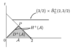
Figure 12. The points of the dashed line belong to $\cup_{t>0}\{t\}\times\hat{B}^{+}_{\Sigma}(2,t)\setminus B^{+}_{\Sigma}(2,t)$ but not to $H^{+}(\mathcal{A})$; the ones of the segment $\overline{0P}$, $0$ excluded, are in $H^{+}(\mathcal{A})$ but not in $\cup_{t>0}\{t\}\times\hat{B}^{+}_{\Sigma}(2,t)$.

8.2. Differentiability of the Randers-Kropina separation

For an $\rm SSTK$ with a causal Killing vector field, we can use the Finslerian separation $d_{F}$ of the associated Randers-Kropina metric to describe the future or the past Cauchy horizon of $\mathcal{A}_{t_{0}}=\{t_{0}\}\times\mathcal{A}$, at least when $S_{0}$ is Cauchy. Indeed, in this case, from Proposition 8.1, the set:

$$\{(t,y)\in\mathds{R}\times M:\not\exists x^{\prime}\in M\setminus{\mathcal{A}}:d_{F}(x^{\prime},y)<t-t_{0}\text{ and }\\ \text{either $y\in\partial\mathcal{A}$, $t\geq t_{0}$ and $\Lambda(y)=0$ or }\exists x\in\partial\mathcal{A}\text{ s. t. }d_{F}(x,y)=t-t_{0}\}\\ =\{(t,y)\in\mathds{R}\times\bar{\mathcal{A}}:\,\hbox{inf}_{x\not\in\mathcal{A}}d_{F}(x,y)=t-t_{0}\}\\ \cup\{(t,x):x\in\partial\mathcal{A},\Lambda(x)=0,\ t\geq t_{0}\,\hbox{and}\not\exists x^{\prime}\in M\setminus\mathcal{A}:d_{F}(x^{\prime},x)<t-t_{0}\}$$

is equal to the horizon $H^{+}({\mathcal{A}}_{t_{0}})$. Notice that, differently from the stationary case, $H^{+}({\mathcal{A}}_{t_{0}})$ might also contain achronal arcs, included in integral curves of $\partial_{t}$, such that $x\in\partial\mathcal{A}$, $\Lambda(x)=0$ and $\mathrm{d}\Lambda(\hbox{Ker}\,\omega_{x})=0$.

Example 8.3.

Consider $\mathds{R}^{2}$ endowed with the flat metric $g=\mathrm{d}x^{2}-(\mathrm{d}x\mathrm{d}t+\mathrm{d}t\mathrm{d}x)/2$ and $\mathcal{A}=(0,1)\subset\mathds{R}$, so that $S_{0}=\{0\}\times\mathds{R}$ is spacelike and the segment connecting the points having coordinates $(0,1)$ and $(1,1)$ (the first coordinate is $t$) is contained in $H^{+}(\mathcal{A}_{0})$. Clearly, this arc cannot be described as made of points belonging to the graph (in $\mathds{R}\times M$) of the function

$$\varphi:=x\in\bar{\mathcal{A}}\mapsto d_{F}(M\setminus\mathcal{A},x),$$

where $d_{F}(M\setminus\mathcal{A},x):=\inf_{y\in M\setminus\mathcal{A}}d_{F}(y,x)$. Modifying this example one can also easily check that, differently from the Riemannian or the Finslerian case, $\varphi$ is not continuous on $\partial\mathcal{A}$, in general.

Following [31], we introduce the notion of future horizon which encompasses some of the essential properties possessed by a Cauchy horizon. A future horizon is a topological, closed, achronal hypersurface ruled by future inextendible lightlike geodesics. This notion allows us to remove the assumption that $S_{0}$ must be a Cauchy hypersurface and, then, to extend to the Randers-Kropina separation $d_{F}$ a result about differentiability of the distance function from a closed subset valid for a Riemannian distance [31, Proposition 11] and for a distance associated with a Randers metric [23, Theorem 5.12].

Let $(M,F)$ be a Randers-Kropina space and $C\subset M$ a closed subset. Let $(\mathds{R}\times M,g)$ be the $\rm SSTK$ splitting associated with $(M,F)$ and $((-\infty,0)\times(M\setminus C),g)$ the spacetime obtained by considering the open subset $(-\infty,0)\times(M\setminus C)\subset\mathds{R}\times M$. Let us define $\rho\colon M\setminus C\to[-\infty,0)$, $\rho(x):=-d_{F}(x,C)$, where, now, $d_{F}(x,C):=\inf_{y\in C}d_{F}(x,y)$. Notice that, similarly to Proposition 4.3, $\rho$ is equal to the function

$$\tau(x) :=\sup\{t\in\mathds{R}:\exists y\in C\text{ such that }(t,x)\ll(0,y)\}$$

$$=\sup\{t\in\mathds{R}:(\{0\}\times C)\cap I^{+}(t,x)\neq\emptyset\}$$

$$=\sup\{t\in\mathds{R}:(t,x)\in I^{-}(\{0\}\times C)\}.$$

Let us prove that $\rho$ is a continuous function ($[-\infty,0)$ is endowed with its natural order topology). Indeed, being $\rho$ defined as minus the infimum of continuous functions, it is lower semi-continuous. Moreover, the following holds too:

Proposition 8.4.

The function $\rho\colon M\setminus C\to[-\infty,0)$ is upper semi-continuous.

Proof.

Assume by contradiction that there exist $x\in M\setminus C$ and two sequences $\{y_{n}\}\subset C$ and $\{x_{n}\}\subset M\setminus C$ such that $x_{n}\rightarrow x$ and $t_{n}:=-d_{F}(x_{n},y_{n})$ satisfy

$$T_{0}:=\lim_{n}t_{n}>\rho(x).$$

Then, take future-pointing timelike curves $\gamma_{n}$ from $(t_{n}-1/n,x_{n})$ to $(0,y_{n})$ and the limit curve $\gamma$ of the sequence starting at $(T_{0},x)$. As $\gamma$ is inextendible and $x\in M\setminus C$, by a reasoning analogous to that in the proof of Theorem 4.5, we deduce that its support cannot be included in the line $l_{x}=\mathds{R}\times\{x\}$. So, take a point $Q$ of $\gamma$ away from $l_{x}$ and $T_{1}\in(\rho(x),T_{0})$. As the line $l_{x}$ is causal, the segment with endpoints $(T_{1},x)$ and $(T_{0},x)$ glued with the arc of $\gamma$ between $(T_{0},x)$ and $Q$ gives a causal curve which cannot be a lightlike pregeodesic (otherwise the line $l_{x}$ would be also a lightlike pregeodesic and, at the first point where $\gamma$ leaves $l_{x}$, uniqueness of geodesics would be violated). Hence, from Remark 3.1, $(T_{1},x)\ll Q$. Being $\gamma$ a limit curve and the relation $\ll$ open, there exists $Q_{\bar{n}}$, $\bar{n}\in\mathds{N}$, belonging to the support of $\gamma_{\bar{n}}$ such that $(T_{1},x)\ll Q_{\bar{n}}$. Therefore, $(T_{1},x)\ll(0,y_{\bar{n}})$ too, and then $T_{1}\leq\rho(x)$, a contradiction. ∎

For each closed set $C\subset M$ we can construct a future horizon by using the function $\rho$ associated with $C$ as follows.

Proposition 8.5.

Let $C\subset M$ be a closed set. Then the hypersurface $H=\{(\rho(x),x):x\in M\setminus C,\rho(x)\neq-\infty\}$ is a future horizon in the spacetime $((-\infty,0)\times(M\setminus C),g)$.

Proof.

Since $\rho:M\setminus C\to[-\infty,0)$ is continuous we get that $H$ is a topological closed hypersurface in $((-\infty,0)\times M\setminus C,g)$. Moreover, it is achronal, otherwise a timelike future-pointing curve would connect $(\rho(x_{1}),x_{1})$ to $(\rho(x_{2}),x_{2})$ and, by taking a sequence of points $\{y_{n}\}\subset C$ such that $(\rho(x_{2})-1/n,x_{2})\ll(0,y_{n})$ we would get $(\rho(x_{1}),x_{1})\ll(0,y_{n})$, for $n$ big enough. Then, for $\varepsilon>0$ small enough, $(\rho(x_{1})+\varepsilon,x_{1})\ll(0,y_{\bar{n}})$, for some $\bar{n}\in\mathds{N}$, which, recalling that $\rho(x_{1})=\tau(x_{1})$, gives a contradiction.

Let us now prove the existence of a future-pointing, future-inextendible, geodesic $\gamma\colon[0,a)\to(-\infty,0)\times M$ through any point of $H$ and contained in $H$. Consider a sequence $\{\gamma_{n}\}$ of timelike future-pointing curves connecting $(\rho(x)-\frac{1}{n},x)$ to $(0,y_{n})$, with $y_{n}\in C$, which we can assume parametrized by the time function $t$. Such a sequence admits a future-pointing limit curve $\gamma\colon[0,a)\to\mathds{R}\times M$, such that $\gamma(0)=(\rho(x),x)$, and we can assume, by taking a smaller $a$ if necessary, that the image of $\gamma$ is contained in $\mathds{R}\times(M\setminus C)$. Reasoning as in the proof of Theorem 4.5 and Proposition 8.4, $\gamma$ cannot be contained in the line $l_{x}$ (as $x\in M\setminus C$) and all the points in $\gamma$ are horismotically related (otherwise, a point $Q$ on $\gamma$ would lie in the chronological future of $(\rho(x),x)$ and, being $\gamma$ a limit curve, this also would imply that $(\rho(x),x)$ is in the chronological past of $C$). From Corollary 5.3, $\gamma$ is a (future inextendible) lightlike pregeodesic which can be parametrized with $t$, i.e., $\gamma(t)=(t,\sigma(t))$, $t\in[\rho(x),t_{1})$ for some $t_{1}>0$ and some unit minimizing $F$-geodesic $\sigma$. To check that $\gamma$ is included in $H$, parametrize also the converging curves as $\gamma_{n}(t)=(t,x_{n}(t))$. Then, for each $t\in[\rho(x),t_{1})$, $t\leq\tau(x_{n}(t))=\rho(x_{n}(t))$ and by the continuity of $\rho$ and Lemma 5.7, $\rho(x_{n}(t))\rightarrow\rho(\sigma(t))$, hence $t\leq\rho(\sigma(t))$. If $t<\rho(\sigma(t))$, there would exist a timelike future-pointing curve connecting $\big{(}t+\rho(\sigma(t))/2,\sigma(t)\big{)}$ to $C$ and then, being the line $l_{\sigma(t)}$ causal, $(\rho(x),x)$ would be in the chronological past of $C$, which is impossible. Thus, $\rho(\sigma(t))=t$ so that $(t,\sigma(t))\in H$. ∎

Actually the proof of Proposition 8.5 shows also that the following extension to Randers-Kropina metrics of [31, Proposition 9] and [23, Proposition 5.11] holds.

Corollary 8.6.

Let $(M,F)$ be a Randers-Kropina space and $C\subset M$ a closed subset. Then every point $x\in M\setminus C$, such that $d_{F}(x,C)<+\infty$, belongs to at least one geodesic segment $\sigma$ which is minimizing, i.e. $d_{F}(\sigma(t),C)=t$, for all $t$ in a certain interval $(t_{0},t_{1}]$ with $\sigma(t_{1})=x$.

The correspondence between lightlike geodesics ruling $H$ and $d_{F}(\cdot,C)$ - minimizing geodesics allows us to use [9, Theorem 3.5], which states that the differentiable points of a horizon are the points which are crossed by one and only one lightlike geodesic ruling the horizon, so that we immediately obtain the following.

Proposition 8.7.

Let $(M,F)$ be a Randers-Kropina space and $C$ a closed subset of $M$. A point $x\in M\setminus C$, such that $d_{F}(x,C)<+\infty$, is a differentiable point of the function $d_{F}(\cdot,C)$ if and only if there exists a unique minimizing geodesic segment of $(M,F)$ through $x$.

Remark 8.8.

Another consequence of the results in [9] is that the set of the points in $M\setminus C$ where $d_{F}(x,C)$ fails to be differentiable is included in the set of the $F$-cut points of $C$, i.e. the points $x\in M\setminus C$ such that a minimizing geodesic through $x$ cannot be extended beyond its beginning at $x$ as a minimizing geodesic. The $F$-cut points of $C$ correspond to the endpoints of $H$ i.e. the points in $H$ where the lightlike geodesics ruling $H$ cease to belong to $H$. Moreover, the set of the points where $d_{F}(\cdot,C)$ is not differentiable corresponds with the crease set of $H$ i.e. the subset of the endpoints of $H$ belonging to two or more ruling lightlike geodesics.

8.3. K-horizons

When the Killing vector field $K$ of an $\rm SSTK$ spacetime is timelike (i.e., in the stationary case), there are no restriction for the admissible curves on the associated Finsler structure; so, each point $p\in\mathds{R}\times M$ and each integral curve of $K$ can be joined by means of a timelike curve $\gamma$. Physically, this prevents the existence of horizons. In fact, if the spacetime admits a sensible notion of future infinity $\mathcal{J}^{+}$ (namely, by means of a conformal embedding [87] or by using the causal boundary [35]), the existence of the connecting curves $\gamma$, the invariance of the metric with the flow of $K$, and the fact that this flow is composed by timelike curves, would imply $I^{-}(\mathcal{J}^{+})=\mathds{R}\times M$. Nevertheless, the situation is different when $K$ changes from timelike to spacelike. This situation is natural in Mathematical Relativity; recall that this happens, for example, in the extension of the Schwarzschild spacetime through its event horizon (the hypersurface $r=2m$, which coincides with the vanishing of $g(K,K)$ for its natural Killing $K=\partial_{t}$) as well as in Kerr spacetime, through the stationary limit hypersurface $H$ that serves as a boundary for the ergosphere (the spacetime event horizon appears beyond $H$).

In general, an embedded hypersurface $H$ invariant by the flow of a Killing vector field $K$ which is tangent and lightlike on $H$ is called a Killing horizon. The regularity of $H$ depends on the context, typically, $0$ would be a regular value of $g(K,K)$, and $H$ would be a connected component of the preimage, but one may admit non-smooth $H$ (see [30, §2.5], [28] and references therein). In the simple case that $H$ is the preimage of a regular value, a naive justification of the name horizon goes as follows. As all the future causal cones must lie on one side of $H$, given $(t_{0},x_{0})\in H$ (regarded as $H=\mathds{R}\times N_{H})(\subset\mathds{R}\times M)$ for some submanifold $N_{H}$) there is a neighborhood $U$ of $x_{0}$ such that no points $p,q\in\mathds{R}\times U$ with $g(K_{p},K_{p})>0,g(K_{q},K_{q})<0$, can be joined by means of a future-pointing (or past-pointing, depending on the time-orientations) timelike curve $\gamma$ from $p$ to $q$ entirely contained in $\mathds{R}\times U$, see Fig. 13 ($\gamma$ could not cross $H$ maintaining its timelike character).

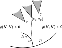
Figure 13. A Killing horizon $H=\mathds{R}\times N_{H}$ with the lightlike cones at $(t_{0},x_{0})\in H$, $p$ and $q$

However, even in this case, one can wonder if $p$ and $q$ could be joined by future-pointing causal curves which leave $\mathds{R}\times U$.

By using the associated Fermat structure $\Sigma$, these considerations can be formulated from a global viewpoint, with independence of the existence of Killing horizons, by means of the following notion.

Definition 8.9.

Let $M$ be a manifold endowed with a wind Finslerian structure $\Sigma$, and let ${\mathcal{A}}\subset M$. The $K$-horizon for $\mathcal{A}$ is the boundary $H_{\Sigma}({\mathcal{A}})$ of the set $\{y\in M:\exists x\in\mathcal{A}\text{ s. t. }C^{A}_{y,x}\neq\emptyset\}$.

Remark 8.10.

When the wind Finslerian structure is a Randers-Kropina metric $F$ with associated separation $d_{F}$, the $K$-horizon for $\mathcal{A}$ can be written as

$$H_{F}({\mathcal{A}})=\partial(\{y\in M:d_{F}(y,{\mathcal{A}})<+\infty\}).$$

When applied to $\rm SSTK$ spacetimes, this yields a natural concept:

Definition 8.11.

Let $(\mathds{R}\times M,g)$ be an $\rm SSTK$ splitting and ${\mathcal{A}}\subset M$. The $K$-horizon for $\mathds{R}\times\mathcal{A}$, is the boundary $H({\mathcal{A}})$ of the set of the points $(t,y)\in\mathds{R}\times M$ such that there exists a future-pointing timelike curve from $(t,y)$ to $\mathds{R}\times{\mathcal{A}}$.

Notice that the $K$-horizons for $\mathcal{A}$ (for both $\Sigma$ and the $\rm SSTK$ splitting) are controlled by the admissible curves and, these, by the open domain $A$ for $\Sigma$. The following results ensure the consistency of the previous two definitions.

Lemma 8.12.

Let $L$ be an $\rm SSTK$ spacetime that splits in two different ways $(\mathds{R}\times M,g),\ (\mathds{R}\times M^{f},g^{f})$ as in Lemma 6.7 and formula (45) for the same Killing vector field $K$, and let $\Sigma$, $\Sigma^{f}$ be the corresponding wind Finslerian structures (according to Convention 6.9 and Proposition 6.10). Consider a subset $\mathcal{A}_{L}\subset L$ invariant by the flow of $K$, and let $\mathcal{A}$ be its projection on $M$ (by using either of the previous two splittings). Then, $H_{\Sigma}(\mathcal{A})=H_{\Sigma^{f}}(\mathcal{A})$.

Proof.

Notice that the $K$-horizons for $\Sigma$ and $\Sigma^{f}$ depends exclusively on the set $A$ of $F$-admissible directions, and these directions are equal for $\Sigma$ and $\Sigma^{f}$, since they are the projections of causal vectors to $M$ and $M^{f}$ (recall that $M^{f}\equiv S^{f}$ can be seen as a hypersurface in $\mathds{R}\times M$ obtained as a graph, see (45)). ∎

Proposition 8.13.

Let $(\mathds{R}\times M,g)$ be an $\rm SSTK$ splitting and ${\mathcal{A}}\subset M$. Then:

1. $H({\mathcal{A}})=\mathds{R}\times H_{\Sigma}({\mathcal{A}})$.

2. The K-horizon $H({\mathcal{A}})$ is included in the region $g(K,K)\geq 0$.

Proof.

The part $(i)$ is a straightforward consequence of the definitions (recall Proposition 5.1). For $(ii)$, if $p\in H({\mathcal{A}})$, $g(K_{p},K_{p})$ cannot be negative as, otherwise, one would have a stationary region $\mathds{R}\times U$ around $p$ ($U\ni p$ open and connected) and all pairs of integral curves of $K$ in this region can be connected by both, future-pointing and past-pointing timelike curves. ∎

Example 8.14.

(Asymptotic flatness). A natural choice of a subset $\mathcal{A}$ for an $\rm SSTK$ splitting is the region $\Lambda>0$, so that $H({\mathcal{A}})$ can be understood as the limit of the region from which one can access to the stationary part $\mathds{R}\times{\mathcal{A}}$. In fact, the standard situation of horizons (including Kerr or Schwarzschild spacetimes) is the following: one considers an $\rm SSTK$ splitting which is asymptotically flat, in the sense that, away from a compact subset, $M$ has one or more ends, each one diffeomorphic to $\mathds{R}^{m}$ with a ball removed, and the associated wind Finslerian structure becomes a Randers metric $F$ approaching asymptotically to the natural Euclidean metric (see [18, Sect. 2.4]). In this case, it is natural to take $\mathcal{A}$ as the exterior of a large ball in one of the ends. Notice that Definition 8.11 gives a natural notion of horizon for that end (in the presence of a Killing field), extendible even when the standard notions of asymptotic flatness cannot be applied.

Remark 8.15.

($K$ horizons vs. Killing horizons). Notice that the strict inequality may hold in the case $(ii)$ of the previous proposition. In fact, this happens in Kerr spacetime for the $K$-horizon $H({\mathcal{A}})$ of the asymptotic region with $\Lambda>0$ (recall that $K$ is spacelike in Kerr’s ergosphere up to the poles). Remarkably, Kerr’s horizon is a $K$-horizon but not a Killing horizon (the stationary limit surface is neither a $K$-horizon nor a Killing horizon).

But even when the equality to 0 holds in $(ii)$, $H({\mathcal{A}})$ can be strictly included in the region $g(K,K)=0$ because of several reasons. First, this region may be not a hypersurface and, for example, it may contain an open subset; this happens in the case of pp-waves, recall Example 4.11. Moreover, when the zero level of $g(K,K)$ is a Killing horizon, the global behavior of the metric may prevent even the existence of a $K$-horizon, see Fig. 14.

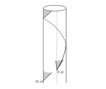
Figure 14. An $\rm SSTK$ cylinder $\mathds{R}\times S^{1}$ with a Killing vector field which is timelike everywhere except at the points of the line passing through $(0,x)$ where it is lightlike; the $K$-horizon $H(\{x\})$ is empty

Summing up, the physical interpretation of the $K$-horizon for $\mathcal{A}$ becomes apparent: $H(\mathcal{A})$ is the limit of the region $R$ so that $\mathds{R}\times\mathcal{A}$ is not accessible for particles starting beyond $R$. So, $K$-horizons are always associated with some concrete $\mathcal{A}$, and are clearly distinct to Killing horizons. Nevertheless, results on spacetimes and Killing horizons may be applicable to $K$-horizons (for example, to ensure that the Kropina part of a wind Finslerian structure appears on a smooth surface and, eventually, may be a $K$-horizon, see Lemma 7 or Proposition 3 in [28]).

9. Conclusions and further developments

To conclude, first we spotlight the distinguishing features of our approach.

When strong wind is considered, there is an obvious failure of the description of Zermelo problem by means of a Finslerian metric of Randers type. The notion of wind-Riemannian structure or, with more generality, wind Finslerian one $\Sigma$, appears then as a natural model even though, as far as we know, the only precedents of such geometric structures are the Kropina-metrics, a particular type of singular Finslerian metrics which would correspond to Zermelo problem with critical wind.

In order to develop the properties of $\Sigma$, a number of new concepts are defined (wind curve, c-ball, w-convexity, etc.), and more standard elements appear: a conic Finsler metric $F$ and a Lorentz-Finsler metric $F_{l}$ on a cone domain. Notably, geodesics in $\Sigma$ split in three types of geodesics: locally minimizing $F$-geodesics, locally maximizing $F_{l}$-geodesics and abnormal geodesics.

For the case of a wind Riemannian structure of dimension $m$, a correspondence with the conformal structure for an $\rm SSTK$ spacetime (a general class of Lorentzian manifolds) of dimension $m+1$ appears. In particular, the cone domain associated with $\Sigma$ can also be interpreted in terms of the (future) causal cone for a Lorentz metric in the region of strong wind (obtained from a sort of projection of the metric in the $\rm SSTK$ splitting), and the abnormal geodesics for $\Sigma$ become lightlike geodesics for this Lorentz metric.

The applications of the correspondence work in both directions. On the one hand, known results in Lorentzian Geometry can be applied to $\rm SSTK$ spacetimes, and they yield a full description of the geodesics of $\Sigma$. In particular, the properties of Kropina and Randers-Kropina metrics can be widely developed. On the other hand, the conformal geometry of an $\rm SSTK$ spacetime can be characterized by means of a wind Riemannian structure in a very precise way. This includes the $\rm SSTK$ causal ladder and the existence of horizons, as well as other properties of more purely mathematical interest such as the existence of some closed geodesics.

This correspondence allows us to obtain a fully satisfactory solution of Zermelo navigation problem with arbitrary wind: roughly, any solution is a geodesic for $\Sigma$, and solutions must exist under w-convexity.

What is more, Zermelo navigation suggests our general version of Fermat’s principle, with independent interest in General Relativity. This general version leads to a unified global variational description of all the $\Sigma$-geodesics connecting two prescribed points of an SSTK spacetime as the critical points of the time arrival functional.

Direct applications of our approach include the modelization of practical situations [63], examples of Analogue Gravity [5, §2] and links with fields where cone structures become relevant, such as Finsler spacetimes [52] or Hamilton-Jacobi equation [34]. What is more, further developments have been carried out by the authors since the first version of the present article. Next, we will mention some of them following four main references, hoping that this may serve as a motivation and guide for readers interested in a variety of related topics.

9.1. Randers and wind Riemannian manifolds of constant flag curvature

(Ref. [53].) The study of Randers manifolds of constant flag curvature (CFC) is a substantial topic in Finslerian Geometry, which includes as a milestone the local and global classification by Bao, Robles and Shen [4]. Essentially, they proved that, for all such metrics, the local Zermelo data $(g_{R},W)$ on $M$ consist of a Riemannian metric $g_{R}$ of constant curvature and a homothetic vector field $W$. Globally, however, a striking difference appears in comparison with the Riemannian case. In the latter, the model spaces (Euclidean, spherical, hyperbolic) appear under the natural assumptions of simple connectedness and completeness. However, in the Randers case, the fact that the $g_{R}$-norm of a homothetic $W$ may be greater and smaller than 1 in different regions of $M$ leads naturally to incomplete examples.

This is solved in [4] by considering inextensible CFC Randers spaces; however, a solution can be given within our more general framework. Indeed, following [53], all the incomplete Randers models can be extended as complete wind Riemannian structures by taking into account our notions of geodesic and completeness developed in Sections 2 and 6.1. Moreover, the notion of CFC can be extended to wind Riemannian structures, being these spaces naturally classifiable now.

Going into detail, we say that a wind Riemannian structure $(M,\Sigma)$ has CFC if its associated conic metrics $F$ and $F_{l}$ have constant flag curvatures for all the flagpoles in $A$ and $A_{l}$, respectively. As a first step, the techniques in [4] remain applicable proving that $(M,\Sigma)$ has constant flag curvature $\kappa\in\mathds{R}$ if and only if its Zermelo data $(g_{R},W)$ satisfy the following two conditions:

• there exists $\mu\in\mathds{R}$ such that the wind $W$ is $\mu$-homothetic for $g_{R}$ (i.e., ${\mathcal{L}}_{W}g_{R}=2\mu g_{R}$, where $\mathcal{L}$ is the Lie derivative), and

• the Riemannian metric $g_{R}$ has constant curvature $\kappa+\frac{1}{4}\mu^{2}$,

see [53, Theorem 3.8]. Using this local result, the following global classification of CFC spaces can be proved, see [53, Theorem 3.12]:

A complete simply connected wind Riemannian structure $(M,\Sigma)$ of constant flag curvature with Zermelo data $(g_{R},W)$ satisfies either

(i) $(M,g_{R})$ is a model space of constant curvature and $W$ is any of its Killing vector fields, or

(ii) $(M,g_{R})$ is isometric to $\mathds{R}^{n}$ and $W$ is a properly homothetic (i.e. non-Killing) vector field.

Along the proof, the following criterion on completeness for $(M,\Sigma)$ is used: if $g_{R}$ is complete and $W$ is homothetic, then $\Sigma$ is complete (moreover, if $W$ is properly homothetic, then $g_{R}$ is flat), see [53, Theorem 3.10-(ii)].

9.2. Sharp criteria on completeness and Cauchy hypersurfaces

(Ref. [54].) From the viewpoint of classical Riemannian or Finslerian Geometries, it was not surprising that completeness was essential for problems of classification; in particular, the criterion cited above goes in this standard direction. However, a major goal in our approach has been to translate properties of the wind Riemannian structure $(M,\Sigma)$ into properties of causality of the associated SSTK spacetime as in Section 5, which opened the possibility of a pletora of relativistic interpretations, including those in Section 8. In this setting, it is especially relevant the equivalence (proven in Theorem 5.9-(iv)) between the completeness of $\Sigma$ and the fact that the slices of its SSTK spacetime are Cauchy hypersurfaces. In [54], completeness is studied motivated by applications to these hypersurfaces. Indeed, a natural characterization of completeness is proven first and, then, criteria to ensure the Cauchy character of the slices are provided, as well as applications to explicit spacetimes. In a nutshell, the idea is that, taking into account only the conic Finsler metric $F$ including its continuous extension to the closure of $A$ in $TM\backslash\mathbf{0}$, Hopf-Rinow type properties will characterize completeness.

More precisely, one considers first an extension of the notion of Finslerian separation in Definition 4.1, obtained by considering the set of wind curves between two given points $C^{\Sigma}_{x_{0},x_{1}}$ and the lengths w.r.t. the extension $\bar{F}$ of $F$ (expressed as in (25)) to $A\cup A_{E}$ (recall Definition 2.11 and Remark 2.61). The notion of geodesic can be quite naturally extended to the conic Finsler manifold $(M,\bar{F})$ (see [54, Definition 3.19]) and, then, also forward and backward completeness are naturally defined for $(M,\bar{F})$. Then, it is proved that $(M,\Sigma)$ is geodesically complete if and only if $(M,\bar{F})$ is geodesically complete. Furthermore, forward (resp. backward) Cauchy completeness of $(M,d_{\bar{F}})$ becomes equivalent to its forward (resp. backward) geodesic completeness which is in turn equivalent to the fact that each closed and forward (resp. backward) bounded subset of $(M,d_{\bar{F}})$ is compact (see [54, Theorem 3.23]). Summing up, applying Theorem 5.9-(iv): the slices $S_{t}$ in the SSTK spacetime $(\mathds{R}\times M,g)$ are Cauchy hypersurfaces iff the associated conic Finsler space $(M,\bar{F})$ is geodesically complete.

Starting at this characterization, it is easy to give sufficient conditions for the completeness of $(M,\Sigma)$ arising from the completeness of some Riemannian or Finslerian metrics whose indicatrix at each $p\in M$ encloses $\Sigma_{p}$, see [54, Props. 4.3 and 4.4, Example 4.6]. Some more refined applications, both relativistic and purely geometric, are also provided. The former include examples of ergospheres and Killing horizons which enhance our study in Section 8.3. Among the latter, it is worth pointing out an example of a Randers manifold $(M,R)$ satisfying the following property: even though not all the closed symmetrized balls of $(M,R)$ are compact, its universal covering $(\tilde{M},\tilde{R})$ satisfies that all its closed symmetrized balls are compact, see [54, Example 2.11]. We emphasize that, for reversible Finsler metrics, the compactness of the closed symmetrized balls is equivalent to its completeness, as a difference with the non-reversible case. Such an example becomes the Finslerian translation of a notable static spacetime obtained by Harris [45]; the underlying ideas in its interpretation come from Section 6.2.

9.3. From wind Finslerian to cones and Lorentz-Finsler metrics

(Ref. [55].) Recall than a wind Finslerian structure $\Sigma$ can always be interpreted using the Zermelo problem, which is now anisotropic in a more general sense that the wind Riemannian case. Indeed, at each point $p\in M$, the subset $\bar{B}_{p}$ enclosed by $\Sigma_{p}=\Sigma\cap T_{p}M$ determines the velocities that a certain moving object can attain at $p$ (see Remark 2.22). If we add a non-relativistic time $t$ as a first coordinate the (non-relativistic) spacetime $\mathds{R}\times M$, the (boundary of the) velocities of the allowed trajectories determine a cone structure $\mathcal{C}$ which at each point $(t,p)$ is given by

$${\mathcal{C}}_{p}=\{\lambda(1,v)\in\mathds{R}\times T_{p}M:\lambda>0,v\in\Sigma_{p}\}.$$ (66)

Observe that this cone can be described by the triple $(dt,\partial_{t},\Sigma)$, being $\Sigma_{p}$ defined in $\ker(dt)\equiv T_{p}M$, (see Fig. 5 for an enlightening picture).

In the above setting, it is very natural to consider a time dependent Zermelo problem, which leads to wind Finslerian structures of the triple $(dt,\partial_{t},\Sigma)$ which depend on the coordinate $t$. Even if we restrict to the wind Riemannian case, an important difference with our approach in terms of SSTK spacetimes would appear, namely, now one cannot expect that the conformal geometry of the spacetime is codified in a single $t$-slice and, thus, a tidy result such as Theorem 5.9 cannot hold. However, the spacetime viewpoint introduced here will be very fruitful to handle these $t$-dependent structures in a unified way. Indeed, to achieve a generalized correspondence for wind Finslerian structures and also time-dependent, we will consider strongly convex cone structures and Lorentz-Finsler metrics [55, Defs. 2.7, 3.5] as the natural generalization of $\rm SSTK$ spacetimes.

As a first observation on cone structures $\mathcal{C}$, they can always be obtained from a class of (anisotropically conformal) Lorentz-Finsler metrics sharing the same pregeodesics, which turn out to be the intrinsic cone geodesics of $\mathcal{C}$ [55, Th. 1.1]. To establish the searched generalization, start at a wind Finslerian structure $(M,\Sigma)$ and construct the cone structure $\mathcal{C}$ as in (66). Then $\mathcal{C}$ can also be regarded as the cone structure of a Lorentz-Finsler metric $L$ on $\mathds{R}\times M$ which admits $K=\partial_{t}$ as a Killing vector field (see some details below). So, we arrive at the natural Finsler generalization of SSTK spacetimes. Recall that the notion of a smooth standard stationary Finsler spacetime has been developed in [55, Def. 4.6]. As in the relativistic case, these spacetimes are also endowed with a standard splitting such that $K=\partial_{t}$ is timelike and Killing. Thus, Finslerian SSTK spacetimes arise just dropping the timelike restriction. Summing up:

1. There is a natural Finslerian generalization of SSTK spacetimes, also endowed with a Killing $K=\partial_{t}$.

2. The further generalization which also permits $t$-dependence is obtained by dropping the Killing character of $\partial_{t}$.

Using the generalization (1), the extension of our full approach is also straightforward. Indeed, by using the intrinsic causal properties of cone structures, the whole setting of Sections 4 to 8 and most of their results are directly transferable. In particular, when $K$ is causal, a notion of Finsler-Kropina metric emerges as a natural extension of Randers-Kropina ones and all the results in Section 4 can be extended to this setting. About (2), some applications will be explained in the next subsection, but the following discussion is convenient first.

In contrast with the Lorentz case, many issues on Lorentz-Finsler metrics and their cone structures have been developed only recently. A detailed study of this general setting as well as of the tools to establish links with the present article is carried out in [55]. Indeed, cone structures are studied both intrinsically and by using a (highly non-unique) cone triple $(\Omega,T,F)$ in a manifold $N$ composed by a 1-form $\Omega$ a timelike vector field $T$ such that $\Omega(T)\equiv 1$ and a Finsler metric $F$ on the kernel of $\Omega$, the latter canonically determined by $\mathcal{C}$ once $\Omega$ and $T$ have been chosen. Observe that at each tangent space of $N$, one can obtain a decomposition $\mathds{R}\times\ker(\Omega)\equiv T_{p}N$ using the vector field $T$ and then an infinitesimal Zermelo problem using the ball of $F$ in $\ker(\Omega)$ as admissible velocities (compare with (66)). Moreover, these elements provide a Lorentz-Finsler metric (which is everywhere smooth but on $T$, where it is smoothable anyway) $L=\Omega^{2}-F^{2}$ and the cone structure $\mathcal{C}$ emerges as the tangent vectors $v$ which are lightlike ($L(v)=0$) and future-directed ($\Omega(v)>0$), see [55, Th. 1.2]. When the manifold splits, the setting of standard stationary spacetimes is naturally reobtained by taking $\Omega=dt$, $T=\partial_{t}$ and $F$ independent of the slice (moreover, a simple description in terms of non-smooth static Finsler spacetimes as in [25] also emerges); obviously, F can also be chosen t-dependent to deal with (2).

Notice, however, that the above description from [55] uses a Finsler metric $F$ rather than a wind Finsler structure $\Sigma$. Nevertheless, there would not be any problem to describe $\mathcal{C}$ by using a triple where $F$ is replaced by $\Sigma$: the latter would also be canonically determined when the restriction of being timelike for $T$ is dropped (recall again (66)). The restriction to a timelike $T$ (or a Finsler $F$) can always be done and gives a simple expression for the Lorentz-Finsler metric $L$, but it is not especially relevant. Indeed, there are cases where a non-necessarily timelike vector field $Z$ with $\Omega(Z)\equiv 1$ appears with independence of $\mathcal{C}$ (for example, when $Z$ is Killing as in the SSTK case or when it represents a priviledged field of observers as in the generalized Zermelo problem below). In these cases, $Z$ may play the role of $\partial_{t}$ and one can use a wind Finslerian structure $\Sigma$ for the description of $\mathcal{C}$.

9.4. Generalizations of Zermelo’s and applications to wave propagation

(Ref. [49].) In accordance with the items (1) and (2) above, the Zermelo navigation problem and Fermat’s principle considered in Sections 6 and 7 admit two natural extensions, namely, when the velocity of propagation is anisotropic (i.e., depending on the direction, beyond the existence of the wind) and time-dependent. Indeed, in [55, Sect. 6], the authors also considered the above Lorentz-Finsler setting, showing that the Zermelo problem reduces to Fermat’s principle and, then, that the cone geodesics of $\mathcal{C}$ provide the solutions for Zermelo’s (notice that, because of time-dependence, the used techniques are different and many of our sharp conclusions for the projections on slices are dropped). Clearly, this setting is applicable to interesting situations as, for example, when the flight time of an airship is affected by a time-dependent wind, eventually strong.

More subtlety, the following application to wave propagation and wildfires, developed in [49] after the work by Markvorsen in [63, 64], holds. Consider a wave which propagates in an anisotropic medium, the latter moving with respect to an observer. For example, when a sound wave propagates in the air, the variations of the properties of this medium such as pressure or temperature may yield an anisotropic speed of propagation with respect to this medium. Moreover, the wind may move the latter and, so, one should add the velocity of the air with respect to Earth to the previous velocity with respect to the medium (one assumes that the observer of the wave would remain at rest on Earth). Of course, the wind, as well as the pressure or temperature, might vary with the space point and the time. From an abstract viewpoint, this is modelled with a cone structure $\mathcal{C}$, eventually described by a cone triple $(\Omega=dt,\partial_{t},\Sigma)$, as explained at the previous subsection. Moreover, in this setting, $\Sigma$ is obtained as the translation of the indicatrix of a Finsler metric $F$ (velocities of the wave without perturbations) by a vector field $W$ (the wind). In this case, $T=W+\partial_{t}$ represents a sort of comoving field of observers, which may be useful for modelling.

When the Zermelo problem is time-dependent, it is no longer possible to reduce the study of its solutions to classical Finsler metrics. A way to solve this problem was firstly introduced by Markvorsen. Motivated by the problem of wildfire propagation, this author introduced a Finsler approach for the time-independent case [63] and, then, he considered rheonomic Lagrange manifolds and frozen metrics for the time-dependent one [64]. The latter would correspond to study $t$-dependent Finsler metrics in the spirit of (2’), but dropping the spacetime viewpoint. This viewpoint is taken into account in [49] so that the “fastest trajectories” followed by the wave (which will yield the frontwave at each instant of time) will become lightlike geodesics of the Lorentz-Finsler metric $L$.

More precisely, the wavefront propagation relies on a Zermelo problem starting from a submanifold rather than from a point. Indeed, in order to compute the evolution of a wave or wildfire, one needs to solve the Zermelo problem from the present wavefront, which will be a codimension 2 submanifold $S_{0}$ (a hypersurface embedded in a slice $t=t_{0}$) of the Finsler spacetime. In particular, Theorem 4.8 in [49] shows that the solutions to this Zermelo problem are given by the lightlike geodesics departing orthogonally from $S_{0}$, at least locally. When the wind is time-independent such geodesics can be computed with a wind Finslerian structure (which is a Finsler metric in the region of mild wind), see [49, Section 6].

Appendix: List of some symbols and conventions

In order to avoid heavy notations, we have made some abuses of notation when there was no possibility of confusion. For the convenience of the reader, the main ingredients of the notation are listed here.

Symbol	Stays for	Reference
$\Sigma$	wind Minkowskian structure on a vector space $V$;	Def. 2.3
	wind Finslerian structure on a manifold $M$ ($\Sigma=\cup_{p}\Sigma_{p}$)	Def. 2.8
$\Sigma_{F}$	indicatrix of a Minkowski norm;	below Def. 2.1
	indicatrix of a Finsler manifold	Remark 2.9
$\tilde{\Sigma}$	reverse wind Finsler structure	Def. 2.17
$M_{mild}$	region of mild wind	Def. 2.11
$M_{crit}$	region of critical wind
$M_{l}$	region of strong wind
$F$	(positively homogeneous) Minkowski norm;	Def. 2.1
	conic pseudo-Minkowski norm, conic Minkowski norm, Lorentzian norm;	Def. 2.4
	Finsler metric; conic pseudo-Finsler metric, Lorentzian Finsler metric;	above Def. 2.8
	conic Finsler metric associated to a wind Finslerian manifold;	Prop. 2.12
	conic Finsler metric associated to a wind Riemannian manifold	Eq. (18)
$F_{l}$	Lorentzian norm associated with a strong wind Minkowskian structure;	Prop. 2.5
	Lorentzian Finsler metric associated to a wind Finslerian manifold;	Prop. 2.12
	Lorentzian Finsler metric associated to a wind Riemannnian manifold	Eq. (22)
$A$	(open) conic domain in a vector space;	Def. 2.4
	domain of a conic Minkowski and a Lorentzian norm associated with a wind Minkowskian structure;	Prop. 2.5
	(open) domain of a wind Finslerian structure ($A=\cup_{p\in M}A_{p}$)	Def. 2.8
$A_{l}=\cup_{p\in M_{l}}A_{p}$	open domain of the conic Finsler metric $F$ and the Lorentzian Finsler metric $F_{l}$ of a strong wind Finslerian structure	Def. 2.11
$A_{E}$	extended domain of wind Finslerian structures	Def. 2.11
	extended definition of $F$ and $F_{l}$ to $A\cup A_{E}$	Conv. 2.19

Symbol	Stays for	Reference
$B$	(open) unit ball for a wind Minkowskian structure	Def. 2.3
$B_{p}$	unit ball for $\Sigma_{p}$	Def. 2.8
$B^{\pm}_{\Sigma}(x_{0},r)$	forward/backward wind balls;	Def. 2.26
$\hat{B}^{\pm}_{\Sigma}(x_{0},r)$	forward/backward c-balls;
$\bar{B}^{\pm}_{\Sigma}(x_{0},r)$	closed forward/backward wind balls
	$\Sigma$-admissible curve;	Def. 2.20-(i)
	$F$-admissible curve;
	wind curve;	Def. 2.20-(ii)
	(strictly) regular curve	Def. 2.20-(iii)
$C^{\Sigma}_{x_{0},x_{1}}$	set of wind curves;	below Ex. 2.23
$C^{A}_{x_{0},x_{1}}$	set of $F$-wind curves;
$\Omega^{A}_{x_{0},x_{1}}$	set of $F$-admissible curves
$C^{\Sigma}_{x_{0},x_{1}}[a,b]$	set of wind curves with domain $[a,b]$	Def. 2.37
$\psi$	wind variation, $F$-wind variation	Def. 2.37
$\ell_{F}$	wind lengths	Def. 2.20-(iv)
$\ell_{F_{l}}$
$d_{F}$	Finslerian separation	Def. 2.24
	unit extremizing (pre)geodesic	Def. 2.35
	minimizing, maximizing, boundary (unit) (pre)geodesic	Def. 2.42
	(pre)geodesic	Def. 2.44
$\gamma_{x_{0}}$	(extremizing) exceptional geodesic at $x_{0}$	Prop. 2.36
		Def. 2.44
	w-convex	Def. 2.45
	geodesically convex	Prop. 2.34
$(L,g)$	Lorentzian ($m+1$)-manifold or spacetime	Subsect. 3.1
$g$	metric of an $\rm SSTK$	Def. 3.2
$g_{R}$	Riemannian metric on $M$
$(g_{0},\omega,\Lambda)$	associated triple to a wind Riemannian structure;	Def. 2.56
	spacelike metric, shift and lapse of an $\rm SSTK$	Prop. 3.3
$S_{t}=$ $\{t\}\times M$	slice of any $\rm SSTK$ spacetime	below Eq. (28)
$\mathds{R}\times TM$	tangent space to $\mathds{R}\times M$ when the $t$-component becomes irrelevant	Conv. 3.5

Symbol	Stays for	Reference
	limit curve	Def. 4.4
		Lem. 5.7
	causal spacetime	Th. 4.9
	strongly causal spacetime;	Rem. 3.4
	stably causal spacetime;
	temporal function
	causally simple spacetime;	Th. 4.9
	globally hyperbolic spacetime;
	Cauchy hypersurface
$h$	signature changing metric on $M$	Eq. (34)
$\tilde{h}$	Lorentzian metric (of index $m-1$) on $M_{l}$ equal to $h/\Lambda^{2}$	Eq. (19)
$M_{\Lambda\neq 0}$	region where $\Lambda$ does not vanish	below Eq. (34)
$\mathcal{N}_{p_{0},\alpha}$	space of lightlike curves from $p$ to the curve $\alpha$	Eq. (48)
$\mathcal{N}_{p_{0},l{{}_{x_{1}}}}$	case when $\alpha$ is the line $l{{}_{x_{1}}}=\{(t,x_{1}):t\in\mathds{R}\}$	below Eq. (59)
$T$	arrival functional;	Eq. (49)
	arrival time functional	above Eq. (59)

References

- [1] R. Abraham and J. E. Marsden, Foundations of Mechanics, Benjamin/Cummings Publishing Co., Inc., Reading, Mass., 1978.
- [2] A. A. Agrachev and Y. L. Sachkov, Control Theory from the Geometric Viewpoint, Encyclopaedia of Mathematical Sciences, 87. Control Theory and Optimization, II. Springer-Verlag, Berlin, 2004.
- [3] F. Antonacci and P. Piccione, A Fermat principle on Lorentzian manifolds and applications, Appl. Math. Lett., 9 (1996), 91–95.
- [4] D. Bao, C. Robles and Z. Shen, Zermelo navigation on Riemannian manifolds, J. Differential Geom., 66 (2004), 377–435.
- [5] C. Barceló, S. Liberati and M. Visser, Analogue Gravity, Living Rev. Relativity, 8 (2005), 12.
- [6] R. Bartolo, A. M. Candela and J. L. Flores, Connectivity by geodesics on globally hyperbolic spacetimes with a lightlike Killing vector field, Rev. Mat. Iberoamericana, 33 (2017), 1–28.
- [7] R. Bartolo, E. Caponio, A.V. Germinario and M. Sánchez, Convex domains of Finsler and Riemannian manifolds, Calc. Var. Partial Differential Equations, 40 (2011), 335–356.
- [8] J. K. Beem, P. E. Ehrlich and K. L. Easley, Global Lorentzian Geometry, Marcel Dekker Inc., New York, second ed., 1996.
- [9] J. K. Beem and A. Królak, Cauchy horizon end points and differentiability, J. Math. Phys., 39 (1998), 6001–6010.
- [10] R. Beig and P. T. Chruściel, Killing initial data, Classical Quantum Gravity, 14 (1997), A83–A92.
- [11] A. N. Bernal and M. Sánchez, Smoothness of time functions and the metric splitting of globally hyperbolic spacetimes, Comm. Math. Phys., 257 (2005), 43–50.
- [12] A. N. Bernal and M. Sánchez, Globally hyperbolic spacetimes can be defined as ‘causal’ instead of ‘strongly causal’, Classical Quantum Gravity, 24 (2007), 745–749.
- [13] L. Biliotti and M. A. Javaloyes, -periodic light rays in conformally stationary spacetimes via Finsler geometry, Houston J. Math., 37 (2011), 127–146.
- [14] O. F. Blanco, M. Sánchez and J. M. M. Senovilla, Structure of second-order symmetric Lorentzian manifolds, J. Eur. Math. Soc., 15 (2013), 595–634.
- [15] R. L. Bryant, Some remarks on Finsler manifolds with constant flag curvature, Houston J. Math., 28 (2002), 221–262.
- [16] A. M. Candela, Lightlike periodic trajectories in space-times, Ann. Mat. Pura Appl. (4), 171 (1996), 131–158.
- [17] A. M. Candela, J. L. Flores and M. Sánchez, Global hyperbolicity and Palais-Smale condition for action functionals in stationary spacetimes, Adv. Math. 218 (2008), 515–536.
- [18] E. Caponio, A. Germinario and M. Sánchez, Convex regions of stationary spacetimes and Randers spaces. Applications to lensing and asymptotic flatness, J. Geom. Anal., 26 (2016), 791–836.
- [19] E. Caponio, F. Giannoni, A. Masiello, and S. Suhr, Connecting and closed geodesics of a Kropina metric, Adv. Nonlinear Stud. 21 (2021), 683–695.
- [20] E. Caponio, M. A. Javaloyes and A. Masiello, Morse theory of causal geodesics in a stationary spacetime, Ann. Inst. H. Poincaré Anal. Non Linéaire, 27 (2010), 857–876.
- [21] E. Caponio, M. A. Javaloyes and A. Masiello, On the energy functional on Finsler manifolds and applications to stationary spacetimes, Math. Ann., 351 (2011), 365–392.
- [22] E. Caponio, M. A. Javaloyes and A. Masiello, Addendum to “Morse theory of causal geodesics in a stationary spacetime via Morse theory of geodesics of a Finsler metric” [Ann. I. H. Poincaré—AN 27 (3) (2010) 857–876], Ann. Inst. H. Poincaré Anal. Non Linéaire, 30 (2013), 961–968.
- [23] E. Caponio, M. A. Javaloyes and M. Sánchez, On the interplay between Lorentzian causality and Finsler metrics of Randers type, Rev. Mat. Iberoamericana, 27 (2011), 919–952.
- [24] E. Caponio and E. Minguzzi, Solutions to the Lorentz force equation with fixed charge-to-mass ratio in globally hyperbolic spacetimes, J. Geom. Phys., 49 (2004), 176–186.
- [25] E. Caponio and G. Stancarone, Standard static Finsler spacetimes, Int. J. Geom. Methods Mod. Phys., 13 (2016), 1650040.
- [26] E. Caponio and G. Stancarone, On Finsler spacetimes with a timelike Killing vector field, Classical Quantum Gravity, 35 (2018), 085007.
- [27] C. Carathéodory, Calculus of Variations and Partial Differential Equations of the First Order, Holden-Day Inc., San Francisco, Calif., 1967.
- [28] A. Carrasco and M. Mars, On marginally outer trapped surfaces in stationary and static spacetimes, Classical Quantum Gravity, 25 (2008), 055011, 19.
- [29] X. Cheng and Z. Shen, Finsler Geometry. An approach via Randers spaces, Science Press Beijing, Beijing; Springer, Heidelberg, 2012,
- [30] P. Chruściel, J. Costa and M. Heusler, Stationary black holes: uniqueness and beyond, Living Rev. Relativity, 15 (2012).
- [31] P. T. Chruściel, J. H. G. Fu, G. J. Galloway and R. Howard, On fine differentiability properties of horizons and applications to Riemannian geometry, J. Geom. Phys., 41 (2002), 1–12.
- [32] P. T. Chruściel and J. D. E. Grant, On Lorentzian causality with continuous metrics, Classical Quantum Gravity, 29 (2012), 145001, 32.
- [33] I. P. Costa e Silva, J. L. Flores, On the splitting problem for Lorentzian manifolds with an -action with causal orbits, Ann. Henri Poincaré, 18 (2017), 1635–167.
- [34] A. Fathi, A. Siconolfi, On smooth time functions, Math. Proc. Cambridge Philos. Soc., 2 (2012), 303–339.
- [35] J. L. Flores, J. Herrera and M. Sánchez, On the final definition of the causal boundary and its relation with the conformal boundary, Adv. Theor. Math. Phys., 15 (2011), 991–1057.
- [36] J. L. Flores, J. Herrera and M. Sánchez, Gromov, Cauchy and causal boundaries for Riemannian, Finslerian and Lorentzian manifolds, Mem. Amer. Math. Soc., 226 (2013), vi+76.
- [37] J. L. Flores and M. Sánchez, The causal boundary of wave-type spacetimes, J. High Energy Phys., (2008), JHEP03(2008)036.
- [38] J. L. Flores and M. Sánchez, Geodesics in stationary spacetimes. Application to Kerr spacetime, Int. J. Theor. Phys., 8 (2002), 319-336.
- [39] D. Fortunato, F. Giannoni and A. Masiello, A Fermat principle for stationary space-times and applications to light rays, J. Geom. Phys., 15 (1995), 159–188.
- [40] F. Giannoni, A. Masiello and P. Piccione, A Morse theory for light rays on stably causal Lorentzian manifolds, Annales de l’I.H.P., section A, 69 (1998), 359–412.
- [41] F. Giannoni, A. Masiello and P. Piccione, The Fermat principle in General Relativity and applications, J. Math. Phys., 43 (2002), 563–596.
- [42] G. Gibbons, C. Herdeiro, C. Warnick and M. Werner: Stationary metrics and optical Zermelo-Randers-Finsler geometry, Phys. Rev. D, 79 (2009), 044022.
- [43] G. Gibbons, and C. Warnick, Traffic noise and the hyperbolic plane, Ann. Phys., 325 (2010), 909–923.
- [44] G. Gibbons, and C. Warnick, The geometry of sound rays in a wind, Contemporary Physics, 52 (2011), 197–209.
- [45] S. G. Harris, Static- and Stationary-complete spacetimes: algebraic and causal structures, Classical Quantum Gravity, 32 (2015), 135026.
- [46] J. Herrera and M. A. Javaloyes, Stationary-complete spacetimes with non-standard splittings and pre-Randers metrics. J. Geom. Phys., 163 (2021), 104120.
- [47] M. A. Javaloyes, Chern connection of a pseudo-Finsler metric as a family of affine connections, Publ. Math. Debrecen, 84 (2014), 29–43.
- [48] M. A. Javaloyes, L. Lichtenfelz and P. Piccione, Almost isometries of non-reversible metrics with applications to stationary spacetimes, J. Geom. Phys., 89 (2015), 38–49.
- [49] M.A. Javaloyes, E. Pendás-Recondo and M. Sánchez. Applications of cone structures to the anisotropic rheonomic Huygens’ principle, Nonlinear Analysis, 209 (2021), 112337.
- [50] M. A. Javaloyes and M. Sánchez, A note on the existence of standard splittings for conformally stationary spacetimes, Classical Quantum Gravity, 25 (2008), 168001, 7.
- [51] M. A. Javaloyes and M. Sánchez, On the definition and examples of Finsler metrics, Ann. Scuola Norm. Sup. Pisa Cl. Sci. (5), 13 (2014), 813–858.
- [52] M. A. Javaloyes and M. Sánchez, Finsler metrics and relativistic spacetimes, Int. J. Geom. Methods Mod. Phys., 11 (2014), 1460032.
- [53] M. A. Javaloyes and M. Sánchez, Wind Riemannian spaceforms and Randers-Kropina metrics of constant flag curvature, Eur. J. Math., 3 (2017), 1225–1244.
- [54] M. A. Javaloyes and M. Sánchez, Some criteria for wind Riemannian completeness and existence of Cauchy hypersurfaces in Lorentzian Geometry and Related Topics, vol. 211 of Springer Proc. Math. Stat., Springer, Cham, 2017, 117–151.
- [55] M. A. Javaloyes and M. Sánchez, On the definition and examples of cones and Finsler spacetimes, RACSAM, 114 (2020), 30.
- [56] M. A. Javaloyes and B. Soares, Geodesics and Jacobi fields of pseudo-Finsler manifolds, Publ. Math. Debrecen, 87 (2015), 5.
- [57] I. Kovner, Fermat principles for arbitrary space-times, Astrophysical Journal, 351 (1990), 114–120.
- [58] T. Levi-Civita, Über Zermelo’s Luftfahrtproblem., Z. Angew. Math. Mech., 11 (1931), 314–322.
- [59] M. Ludvigsen, General Relativity. A Geometric Approach., Cambridge Univ. Press, Cambridge, 2004.
- [60] L. A. Lyusternik and A. I. Fet, Variational problems on closed manifolds, Doklady Akad. Nauk SSSR (N.S.), 81 (1951), 17–18.
- [61] D. Maerten, Killing initial data revisited, J. Math. Phys., 45 (2004), 2594–2599.
- [62] B. Manià, Sopra un problema di navigazione di Zermelo, Math. Ann., 113 (1937), 584–599.
- [63] S. Markvorsen, A Finsler geodesic spray paradigm for wildfire spread modelling, Nonlinear Anal. Real World Appl., 28 (2016), 208–228.
- [64] S. Markvorsen. Geodesic sprays and frozen metrics in rheonomic Lagrange manifolds, arXiv:1708.07350 [math.DG], (2017).
- [65] M. Mars and M. Reiris, Global and uniqueness properties of stationary and static spacetimes with outer trapped surfaces, Comm. Math. Phys., 322 (2013), 633–666.
- [66] A. Masiello and P. Piccione, Shortening null geodesics in Lorentzian manifolds. Applications to closed light rays, Differential Geom. Appl., 8 (1998), 47–70.
- [67] H.-H. Matthias, Zwei Verallgemeinerungen eines Satzes von Gromoll und Meyer, Dissertation, Rheinische Friedrich-Wilhelms-Universität, Bonner Mathematische Schriften, Bonn, 1980.
- [68] V. S. Matveev, Can we make a Finsler metric complete by a trivial projective change?, in Recent trends in Lorentzian geometry, vol. 26 of Springer Proc. Math. Stat., Springer, New York, 2013, 231–242.
- [69] E. Minguzzi, On the existence of maximizing curves for the charged-particle action, Classical Quantum Gravity, 20 (2003) 4169–4175.
- [70] E. Minguzzi and M. Sánchez, Connecting solutions of the Lorentz force equation do exist, Comm. Math. Phys., 264 (2006), 349–370.
- [71] E. Minguzzi and M. Sánchez, The causal hierarchy of spacetimes, in Recent developments in pseudo-Riemannian geometry, ESI Lect. Math. Phys., Eur. Math. Soc., Zürich, 2008, 299–358.
- [72] B. O’Neill, Semi-Riemannian Geometry, Academic Press Inc. , New York, 1983.
- [73] B. O’Neill, The geometry of Kerr black holes. A K Peters, Ltd., Wellesley, MA, 1995.
- [74] V. Perlick, On Fermat’s principle in general relativity. I. The general case, Classical Quantum Grav., 7 (1990), 1319–1331.
- [75] V. Perlick, Gravitational lensing from a spacetime perspective, Living Rev. Relativity,(2004).
- [76] H.-B. Rademacher, Nonreversible Finsler metrics of positive flag curvature, in A sampler of Riemann-Finsler geometry, vol. 50 of Math. Sci. Res. Inst. Publ., Cambridge Univ. Press, Cambridge, 2004, 261–302.
- [77] M. Sánchez, Some remarks on causality theory and variational methods in Lorentzian manifolds, Conf. Semin. Mat. Univ. Bari, 265 (1997).
- [78] M. Sánchez, Timelike periodic trajectories in spatially compact Lorentz manifolds, Proc. Amer. Math. Soc., 127 (1999), 3057–3066.
- [79] M. Sánchez, On causality and closed geodesics of compact Lorentzian manifolds and static spacetimes, Differential Geom. Appl., 24 (2006), 21–32.
- [80] U. Serres, Geometry and feedback classification of low-dimensional non-linear control systems. Mathematics [math]. Université de Bourgogne, 2006. English. tel-00172902. Available at https://tel.archives-ouvertes.fr/tel-00172902
- [81] Z. Shen, Lectures on Finsler Geometry, World Scientific Publishing Co., Singapore, 2001.
- [82] Z. Shen, Finsler metrics with and , Canad. J. Math., 55 (2003), 112–132.
- [83] M. Tanaka and S. V. Sabau, The cut locus and distance function from a closed subset of a Finsler manifold, Houst. J. Math., 42 (2016), 1157–1197.
- [84] F. J. Tipler, Existence of closed timelike geodesics in Lorentz spaces, Proc. Amer. Math. Soc., 76 (1979), 145–147.
- [85] K. Uhlenbeck, A Morse theory for geodesics on a Lorentz manifold., Topology, 14 (1975), 69–90.
- [86] R. von Mises, Zum Navigationsproblem der Luftfahrt., Z. f. angew. Math., 11 (1931), 373–381.
- [87] R. M. Wald, General Relativity, University of Chicago Press, Chicago, IL, 1984.
- [88] J. Whitehead, Convex regions in the geometry of paths, Q. J. Math., Oxf. Ser., 3 (1932), 33–42, with an addendum.
- [89] R. Yoshikawa and S. V. Sabau, Kropina metrics and Zermelo navigation on Riemannian manifolds, Geom. Dedicata, 171 (2014), 119-148.
- [90] E. Zermelo, Über das Navigationsproblem bei ruhender oder veränderlicher Windverteilung., Z. Angew. Math. Mech., 11 (1931), 114–124.