Equivalence testing for functional data with an application to comparing pulmonary function devices

Abstract

Equivalence testing for scalar data has been well addressed in the literature, however, the same cannot be said for functional data. The resultant complexity from maintaining the functional structure of the data, rather than using a scalar transformation to reduce dimensionality, renders the existing literature on equivalence testing inadequate for the desired inference. We propose a framework for equivalence testing for functional data within both the frequentist and Bayesian paradigms. This framework combines extensions of scalar methodologies with new methodology for functional data. Our frequentist hypothesis test extends the Two One-Sided Testing (TOST) procedure for equivalence testing to the functional regime. We conduct this TOST procedure through the use of the nonparametric bootstrap. Our Bayesian methodology employs a functional analysis of variance model, and uses a flexible class of Gaussian Processes for both modeling our data and as prior distributions. Through our analysis, we introduce a model for heteroscedastic variances within a Gaussian Process by modeling variance curves via Log-Gaussian Process priors. We stress the importance of choosing prior distributions that are commensurate with the prior state of knowledge and evidence regarding practical equivalence. We illustrate these testing methods through data from an ongoing method comparison study between two devices for pulmonary function testing. In so doing, we provide not only concrete motivation for equivalence testing for functional data, but also a blueprint for researchers who hope to conduct similar inference.

FLA

and

1 Introduction

An equivalence test is a statistical hypothesis test whose inferential goal is to establish practical equivalence rather than a statistically significant difference [Berger and Hsu (1996)]. These tests arise from the fact that within the frequentist paradigm, failing to reject a null hypothesis of no difference is not logically equivalent to accepting said null. Examples of scenarios requiring equivalence tests include the assessment of a generic drug’s performance relative to a brand name drug and method comparison studies, in which the agreement of a new device with the “gold-standard” for measuring a particular phenomenon must be assured before the new device can replace the old one.

Equivalence tests for scalar data typically involve the establishment of upper and lower equivalence thresholds dependent on the metric of equivalence being used. The inferential aim is to establish that the metric falls within the upper and lower equivalence thresholds with a prespecified Type I error rate. See Berger and Hsu (1996) for a comprehensive overview of commonly used procedures. Oftentimes the use of scalar data is adequate, but in some instances the question of practical equivalence cannot be reduced to a hypothesis regarding scalar data.

The motivation for this research arose from a method comparison study between a new device for assessing pulmonary function, Structured Light Plethysmography (SLP), and the industry standard for such assessments, a spirometer. SLP holds many advantages over spirometry: it is noninvasive, it can be used to diagnose patients of a wider range of age and health levels, and it provides detailed information regarding specific regions of the lung that may be malfunctioning. Before SLP may be used extensively for diagnostic purposes it must be assured beyond a reasonable doubt that the measurements obtained by SLP are practically equivalent to those produced by a spirometer.

Doctors rely on a host of information that can be produced both by SLP and by spirometry. Some of these measurements are scalar and, hence, their equivalence can be addressed using available scalar methods; however, not all diagnostic tools utilized are scalar. For example, the “Flow-Volume Loop” is a phase plot of flow of air into and out of the lungs versus volume of air within the lungs over time for each breath. This plot allows doctors to investigate the relationship between flow and volume at various points in time during a given breath, which can indicate whether one has normally functioning lungs, suffers from an obstructive airway disease (such as asthma), suffers from a restrictive lung disease (such as certain types of pneumonia), or rather has another condition altogether. In fact, certain pulmonary ailments are associated with certain shapes of these loops. Figure 1 shows Flow-Volume Loops for healthy patients and for patients with varying pulmonary ailments [Goudsouzian and Karamanian (1984)].

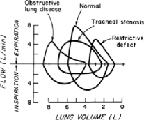
Figure 1: Flow-Volume Loops corresponding to various levels of pulmonary health, calculated using a spirometer. [Reproduced from Goudsouzian, N. and Karamanian, A. (1984). Physiology for the Anesthesiologist, 2nd ed. Appleton-Century-Crofts, Norwalk, CT, with permission.]

Alberola-Lopez and Martin-Fernandez (2003) discuss a frequentist approach for comparing two functions through the use of a Fourier basis expansion. Behseta and Kass (2005) propose a Bayesian method for assessing the equality of two functions using a nonparametric regression method known as Bayesian adaptive regression splines (BARS). Neither of these approaches uses the idea of establishing practical equivalence; rather, both papers test strict equality between the functions of interest, and in fact set strict equality as the null hypothesis and lack thereof as the alternative. In this paper, we propose a framework for functional equivalence testing that is analogous to its univariate counterpart. This involves an extension of scalar techniques to the functional realm and a modification of said techniques when a simple extension is not possible. In so doing, the inferential objective becomes to establish that a functional metric of equivalence lies within a tolerance region with a prespecified Type I error rate. We then discuss methods for equivalence testing within the frequentist and Bayesian paradigms, and illustrate these techniques with data from the method comparison study between SLP and spirometry. We further introduce a Bayesian model for heteroscedastic functional data inspired by the work of Barnard, McCulloch and Meng (2000) that separately places priors on the correlation structure and the underlying variance functions.

2 A framework for equivalence testing

2.1 Equivalence testing for scalar data

In the scalar case, equivalence testing begins by defining a metric whose value can be used to assess equivalence between the two populations of interest, say, $\theta$. Common choices include the difference between group means, $\mu_{1}-\mu_{2}$, and the difference of logarithms of group means, $\log(\mu_{1})-\log(\mu_{2})$ (provided one’s data are strictly positive). One then chooses lower and upper thresholds, $\kappa_{l}$ and $\kappa_{u}$, such that we can reject or fail to reject nonequivalence depending on whether or not $\theta$ falls between $\kappa_{l}$ and $\kappa_{u}$. The null hypothesis is nonequivalence and the alternative is equivalence:

$${\mathbf{H}}_{\mathbf{0}}\dvtx\theta\notin(\kappa_{l},\kappa_{u}),$$

$${\mathbf{H}}_{\mathbf{a}}\dvtx\theta\in(\kappa_{l},\kappa_{u}).$$

A common approach for conducting this hypothesis test within the frequentist paradigm is known as a Two One-Sided Test (TOST) [Berger and Hsu (1996)]. As the name suggests, this is a two step procedure. In no particular order, one separately tests for the alternatives that $\theta<\kappa_{u}$ and $\theta>\kappa_{l}$ with each test being conducted with size $\alpha$. If one successfully rejects for both tests, practical equivalence may then be suggested at size $\alpha$; otherwise, one fails to suggest practical equivalence. The lack of compensation in the significance level of the individual tests (say, to $\alpha/2$) follows immediately from the theory of Intersection-Union Tests (or IUTs), which are tests for which the null parameter space can be described as the union of disjoint sets, and the alternative as the intersection of the complements of those sets. One can see that an equivalence test is an IUT [Berger (1982)], as its null region is $\Theta_{0}:=\{(-\infty,\kappa_{l}]\cup[\kappa_{u},\infty)\}$ and its alternative region is $\Theta_{a}:=(\kappa_{l},\kappa_{u})=\Theta_{0}^{c}$.

The TOST testing procedure can suffer from a lack of power. Brown, Hwang and Munk (1995) and Berger and Hsu (1996) propose procedures which are uniformly more powerful for the scalar case, however, these methods are themselves quite complicated even when dealing with univariate data, to such an extent that TOST continues to be the method of choice in the vast majority of applications. We proceed within the TOST framework, which not only has intuitive appeal but can also be naturally extended to a test of equivalence for functional data within the frequentist paradigm.

The most common goal of equivalence testing is to prove equivalence of means, but this may not be sufficient. Anderson and Hauck (1990) and Chow and Liu (1992) both suggest that in addition to comparing mean responses, the variance of the two responses should also be compared, as a device or drug with smaller variability may be preferred. We will thus include a test for equivalence of variance in our testing procedure.

2.2 Equivalence testing for functional data

We now extend the equivalence testing framework to the functional regime. Let $\theta(\cdot)$ denote a functional measurement of similarity between the location parameters of two functions. One potential choice for $\theta(\cdot)$ is the difference between overall mean functions. $\mu_{1}(\cdot)-\mu_{2}(\cdot)$, but the choice of $\theta(\cdot)$ should depend on the nature of the inference being conducted. Let $\kappa_{l}(\cdot)$ and $\kappa_{u}(\cdot)$ denote lower and upper equivalence bands, which again vary over the same continuum as do the functional data. These bands are chosen such that practical equivalence can be suggested or refuted depending on whether or not $\theta(\cdot)$ falls entirely within $\kappa_{l}(\cdot)$ and $\kappa_{u}(\cdot)$.

For testing the equivalence of variability of the functional data, let $\lambda(\cdot)$ be a measurement of similarity between spreads of the populations. Choices may include $\frac{\sigma^{2}_{1}(\cdot)}{\sigma^{2}_{2}(\cdot)}$, the ratio between the variance functions of the two populations, or $\sigma^{2}_{1}(\cdot)-\sigma^{2}_{2}(\cdot)$, the difference between the two variances. We again establish upper and lower bands, $\zeta_{l}(\cdot)$ and $\zeta_{u}(\cdot)$, within which we can suggest practical equivalence of variance functions.

The null and alternative hypotheses for the tests of location and spread can then be stated as follows:

Note that the above test, in aggregate, is an IUT; the alternative space is $\{\theta(\cdot),\lambda(\cdot)\dvtx\forall t\in\mathcal{T},\theta(t)\in(\kappa_{l}(t),\kappa_{u}(t))\cap\lambda(t)\in(\zeta_{l}(t),\zeta_{u}(t))\}$. In order to test these hypotheses within the frequentist paradigm, we propose conducting two TOST procedures, one each for the location and spread parameters. Since this is an IUT, each of the four total hypothesis tests can be conducted at significance level $\alpha$ to arrive at an overall size of $\alpha$. Details of our frequentist testing procedure can be found in Section 4. Sections 8 and 9 also discuss conducting this test as a Bayesian.

Falling outside of the equivalence region for variability need not be a condemnation; to the contrary, whichever population has markedly smaller variability could be favored on those grounds. If one were comparing a gold standard to a new device and the new device had markedly lower variation, that would strengthen the case for the introduction of the new device into the market. Hence, in the case of method comparison studies, a simple one-sided test of noninferiority may be sufficient for comparing residual variability.

Note that, in practice, functional data are measured along a finite grid of values. Thus, the grid must be fine enough such that areas of potential dissimilarity along the domain are not ignored.

3 Equivalence testing for volume over time functions

As was explained in Section 1, we are interested in whether or not the Flow-Volume Loops produced by spirometry are practically equivalent to those produced by SLP in terms of location and variability. Measurements for volume over time and flow over time were recorded in 2009 for 16 individuals, with the devices set up such that each breath was simultaneously recorded by SLP and spirometry. These data were not the result of a clinical trial and, hence, our use of the data serves exposition of our methodology rather than an argument for the equivalence of SLP and spirometry. Our analysis herein focuses on using the 453 pairs of volume over time curves measured by both devices on these 16 patients to assess the equivalence of SLP and spirometry. Figure 2 shows the visual correspondence between these volume over time plots for SLP and spirometry from an individual.

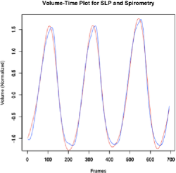
Figure 2: Volume over time obtained using SLP and spirometry for an individual.

The data require preprocessing before our analysis can proceed, as we must break our recordings into individual breaths that are aligned between devices and that are comparable in terms of their domains and scale; see the supplementary materials [Fogarty and Small (2014)] for details. This results in 453 pairs of breaths, where each breath is measured at 25 equispaced time points, time is scaled to the interval $[0,1]$, and time $t$ for SLP corresponds with time $t$ for spirometry within each pair to the best of our ability.

3.1 A model for volume over time functions

We use a functional analysis of variance model with cross-covariance between pairs of functions for our data. Functional analysis of variance models are appropriate when one’s data are comprised of functional responses that are believed to differ from one another solely due to certain categorical variables [Ramsay and Silverman (2005)]. Our model states that we can express the measured volume in the lungs of person $i$ using both devices (denoting SLP by $1$ and spirometry by $2$) in the $k$th breath at time $t\in\mathcal{T}$ as follows:

$$\left[\begin{array}[]{c}\mathbf{v}_{i,1,k}(t)\\ \mathbf{v}_{i,2,k}(t)\end{array}\right] = \left[\begin{array}[]{c}\alpha_{i,1}(t)\\ \alpha_{i,2}(t)\end{array}\right]+\left[\begin{array}[]{c}\epsilon_{i,1,k}(t)\\ \epsilon_{i,2,k}(t)\end{array}\right],$$

$$\left[\begin{array}[]{c}\alpha_{i,1}(t)\\ \alpha_{i,2}(t)\end{array}\right] = \left[\begin{array}[]{c}\mu_{1}(t)\\ \mu_{2}(t)\end{array}\right]+\left[\begin{array}[]{c}\varepsilon_{i,1}(t)\\ \varepsilon_{i,2}(t)\end{array}\right].$$

In this model $[\mu_{1}(\cdot),\mu_{2}(\cdot)]$ represent the overall mean volume over time trajectory for each device. We model the pairs $\{[\alpha_{i,1}(\cdot),\alpha_{i,2}(\cdot)]\}$ as random effects, as we think of the individuals as draws from a larger population. The terms $\{[\epsilon_{i,1,k}(\cdot),\epsilon_{i,2,k}(\cdot)]\}$ are the mean zero error functions for the realized volume over time trajectory of each pair of devices, assumed to be independent between breaths while allowing for both strong autocorrelation along the domain of a given breath and cross-correlation between two breaths in a given pair. This means that not only is there correlation between the value of the functions at times $t$ and $t^{\prime}$ for each breath from a specific device, but there will also be a correlation between the observation at time $t$ from SLP and the observation at time $t^{\prime}$ from the spirometer. Denote the variance functions of these errors by $[\sigma^{2}_{\epsilon,1}(\cdot),\sigma^{2}_{\epsilon,2}(\cdot)]$. The terms $\{[\varepsilon_{i,1}(\cdot),\varepsilon_{i,2}(\cdot)]\}$ are the mean zero error functions for each patient’s pair of random effects, assumed to be independent between patients while allowing for both strong autocorrelation along the domain of a given breath and cross-correlation between random effects in a given pair. Denote the variance functions of these random effects by $[\sigma^{2}_{\alpha,1}(\cdot),\ \sigma^{2}_{\alpha,2}(\cdot)]$.

3.2 Defining equivalence bands

For our analysis, we define $\theta(\cdot)\triangleq\mu_{1}(\cdot)-\mu_{2}(\cdot)$, $\lambda(\cdot)\triangleq\sigma^{2}_{\epsilon,1}(\cdot)/\sigma^{2}_{\epsilon,2}(\cdot)$. In addition, we want to assure ourselves that the variabilities of the random effect functions are similar between the two populations; otherwise, there may be evidence of a systematic bias. As such, we define a third metric of equivalence as $\psi(\cdot)\triangleq\sigma^{2}_{\alpha,1}(\cdot)/\sigma^{2}_{\alpha,2}(\cdot)$. Research is currently being conducted to ascertain proper values for upper and lower equivalence bands for our measures of equivalence of location and spread. These equivalence bands must be established via consultation of field experts (in our case, with pulmonary specialists). For the purpose of illustrating the methodology outlined herein, however, we set reasonable equivalence bands based on the fact that the time points immediately before, during, and immediately after maximal volume is attained are critical for diagnostic purposes: $\kappa_{l}(t)\triangleq-0.05\cos(2\pi t)-0.15$; $\kappa_{u}(t)\triangleq 0.05\cos(2\pi t)+0.15$; $\zeta_{u}(t)\triangleq 0.1\cos(2\pi t)+1.8$; $\zeta_{l}(t)\triangleq 1/(0.1\cos(2\pi t)+1.8)$.

We use the same sets of equivalence bands for the error variances and the random effect variances, although in practice these should be chosen separately. The class of equivalence bands need not be symmetric, as this assumption may be unrealistic; we have merely done so for simplicity. Figure 3 shows the locational discrepancy between volume curves if the true differences between devices truly were at the upper and lower thresholds of equivalence we have specified.

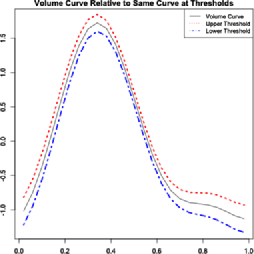
Figure 3: A Volume curve and the corresponding curve with $\kappa_{l}(\cdot)$ and $\kappa_{u}(\cdot)$ applied.

4 Frequentist equivalence testing for functional data

We propose using the nonparametric bootstrap [Efron and Tibshirani (1993)] for assessing equivalence by constructing pointwise confidence intervals for each metric of equivalence, and then using the duality between confidence intervals and pointwise hypothesis tests to conduct our inference. We begin with a testing procedure for i.i.d. data, as we imagine many situations encountered in practice will be of this form. We then discuss a procedure for testing within a random effects model. Allowing for random effects is useful for repeated measures data such as our pulmonary device data. Through our exposition, we illustrate why pointwise coverage of our confidence intervals is actually sufficient for guaranteeing that the resultant inference is of the desired size.

4.1 IID data, independence between populations

We use the difference in mean functions, $\theta(\cdot)\triangleq\mu_{1}(\cdot)-\mu_{2}(\cdot)$ and the ratio of variance functions $\lambda(\cdot)\triangleq\frac{\sigma^{2}_{\epsilon,1}(\cdot)}{\sigma^{2}_{\epsilon,2}(\cdot)}$, as metrics for equivalence. Let $y_{1,1}(\cdot),\ldots,y_{1,n_{1}}(\cdot)$ and $y_{2,1}(\cdot),\break\ldots,y_{2,n_{2}}(\cdot)$ denote the $n_{1}$ and $n_{2}$ observations from groups 1 and 2, respectively, and let $\bar{y}_{1}(\cdot)-\bar{y}_{2}(\cdot)$ denote the sample mean functions.

We use $\hat{\theta}(\cdot)\triangleq\bar{y}_{1}(\cdot)-\bar{y}_{2}(\cdot)$ and $\hat{\lambda}(\cdot)\triangleq\frac{s^{2}_{\epsilon,1}(\cdot)}{s^{2}_{\epsilon,2}(\cdot)}$ as our test statistics for the hypothesis test, and use the nonparametric bootstrap to derive pointwise confidence intervals for the corresponding parameters. We then use the duality between one-sided confidence intervals and one-sided tests to reject or fail to reject nonequivalence.

In each bootstrap simulation, we do the following: [4.]

Sample $n_{1}$ curves with replacement from the curves in group 1, and sample $n_{2}$ curves with replacement from the modified curves in group 2.

Compute the pointwise mean curve from these samples and the pointwise variance curves for each population. Denote these as $\{\bar{y}^{*}_{i}(\cdot)\}$ and $\{s^{2*}_{i}(\cdot)\}$.

Compute $\hat{\theta}^{*}(\cdot)\triangleq\bar{y}^{*}_{1}(\cdot)-\bar{y}^{*}_{2}(\cdot)$ and $\hat{\lambda}^{*}(\cdot)\triangleq\frac{s^{2*}_{1}(\cdot)}{s^{2*}_{2}(\cdot)}$.

Store this value.

Next, we find upper and lower one-sided pointwise $100(1-\alpha)$ confidence intervals. Let $q_{p}[X(t)]$ denote the $p$-quantile for the distribution of $X$ evaluated at time $t$. Then, we define our upper and lower pointwise confidence intervals for $\theta(t)$ using a bias correcting percentile-based bootstrap as discussed in Davison and Hinkley (1997):

$$C^{u}_{1-\alpha}\bigl{(}\theta(t)\bigr{)} = \bigl{[}2\hat{\theta}(t)-q_{\alpha}\bigl{[}\hat{\theta}^{*}(t)\bigr{]},\infty\bigr{)},$$

$$C^{l}_{1-\alpha}\bigl{(}\theta(t)\bigr{)} = \bigl{(}-\infty,2\hat{\theta}(t)-q_{1-\alpha}\bigl{[}\hat{\theta}^{*}(t)\bigr{]}\bigr{)}.$$

At any particular poin $t$, $C^{u}_{1-\alpha}(\theta(t))$ and $C^{l}_{1-\alpha}(\theta(t))$ can be interpreted as the set of all $\theta_{0}$ such that we fail to reject the null that $\theta(t)\leq\theta_{0}$ and $\theta(t)\geq\theta_{0}$, respectively. As such, if our lower equivalence band at time $t$, $\kappa_{l}(t)$, is outside of $C^{u}_{1-\alpha}(\theta(t))$, then we can reject the null that $\theta(t)\leq\kappa_{l}(t)$ at the point $t$. Likewise, if $\kappa_{u}(t)$ is outside of $C^{l}_{1-\alpha}(\theta(t))$, then we can reject the null that $\theta(t)\geq\kappa_{l}(t)$ at the point $t$.

Our upper and lower pointwise confidence interval for $\lambda(t)$ take on a different form. This is because dispersion measures are not typically variance stabilized. In such cases, conventional bootstrap intervals fail to attain their advertised coverage probabilities in small samples. We imagine that most test statistics for testing equivalence of dispersion will be based on the sample variance. For many distributions (including the normal), transforming by the logarithm results in an estimator whose variance is stabilized. Hence, we instead construct upper and lower one-sided confidence intervals for the variance stabilized quantity $\log(\lambda(t))$, and then utilize the monotonicity of the log transform to result in confidence intervals for $\lambda(t)$,

$$C^{u}_{1-\alpha}\bigl{(}\lambda(t)\bigr{)} = \bigl{[}\bigl{(}\hat{\lambda}(t)\bigr{)}^{2}\times q_{1-\alpha}\bigl{[}1/\hat{\lambda}^{*}(t)\bigr{]},\infty\bigr{)},$$

$$C^{l}_{1-\alpha}\bigl{(}\lambda(t)\bigr{)} = \bigl{(}0,\bigl{(}\hat{\lambda}(t)\bigr{)}^{2}\times q_{\alpha}\bigl{[}1/\hat{\lambda}^{*}(t)\bigr{]}\bigr{]}.$$

These intervals can be used to test whether $\lambda(t)$ is below the upper equivalence band and above the lower equivalence band at any point $t$. If one is concerned about the log transform providing variance stabilization, another approach to constructing these confidence intervals would be to estimate a variance stabilizing transformation within the bootstrap framework [see Davison and Hinkley (1997), Tibshirani (1988)].

We now have tests for whether or not we have equivalence of location and spread at any point $t$. To test for overall equivalence, we conduct tests at each domain point based on the $100(1-\alpha)$ pointwise interval at all points $t\in\mathcal{T}$ and reject the null of nonequivalence only if all of the individual tests result in a rejection. To see why there is no need to correct for simultaneous comparisons, let $\mathcal{T}_{0}\cup\mathcal{T}_{a}=\mathcal{T}$ be a partition of the domain where $\mathcal{T}_{0}$ contains the points for which the null hypothesis is true and $\mathcal{T}_{a}$ contains the points for which the alternative is true for any true metric of equivalence in the set of nonequivalence. Then, the probability of a false rejection is bounded as follows:

$$\mathbb{P}(\mbox{Type I error}) = \mathbb{P}(\mbox{falsely reject all of }\mathcal{T}_{0},\mbox{correctly reject all of }\mathcal{T}_{a})$$

$$\leq \mathbb{P}(\mbox{falsely reject all of }\mathcal{T}_{0})$$

$$\leq \mathbb{P}(\mbox{falsely reject a particular }t_{0}\in\mathcal{T}_{0})$$

$$= \alpha.$$

Hence, pointwise $\alpha$ tests of hypothesis guarantee size of at most $\alpha$. In fact, if one had further information regarding the correlation between test statistics, these tests could be done at a size larger than $\alpha$, since our decision to reject nonequivalence is an intersection of tests. As an example, if our function were defined on a grid of size $|\mathcal{T}|=20$, our test statistics were independent, and we wanted an overall size of $\alpha=0.05$, we could then run our tests using $\alpha^{*}=\alpha^{1/20}=0.87$. In the absence of such knowledge, conducting the pointwise tests at size $\alpha$ is actually a tight upper bound. To see this, consider an equivalence metric that is in the equivalence region at all points along the domain except for $t_{0}$, at which its value equals that of the equivalence band. If the probabilities of correct rejection at all points $\mathcal{T}/\{t_{0}\}$ are sufficiently close to one, then essentially the type one error rate is the size of the test at $t_{0}$, which is $\alpha$. In Section 10.1, we give an example where the overall size approaches the upper bound $\alpha$.

4.2 IID matched pairs

For paired functions (commonly arising in comparison studies where simultaneous measurements using two devices are possible), slight alterations are required in the bootstrapping procedure. We again use the difference in mean functions, $\theta(\cdot)\triangleq\mu_{1}(\cdot)-\mu_{2}(\cdot)$ and the ratio of variance functions $\lambda(\cdot)\triangleq\frac{\sigma^{2}_{1}(\cdot)}{\sigma^{2}_{2}(\cdot)}$, as metrics for equivalence. Let $\{y_{1,i}(\cdot),y_{2,i}(\cdot)\}$ be the paired curves, and let $n$ denote the total number of pairs. The bootstrap procedure is as follows: [4.]

Sample $n$ pairs of curves with replacement from the original sample.

Compute the pointwise mean curve from these samples and the pointwise variance curves for each population. Denote these as $[\bar{y}^{*}_{1}(\cdot),\bar{y}^{*}_{2}(\cdot)]$ and $[s^{2*}_{1}(\cdot),s^{2*}_{2}(\cdot)]$.

Compute $\hat{\theta}^{*}(\cdot)\triangleq\bar{y}^{*}_{1}(\cdot)-\bar{y}^{*}_{2}(\cdot)$ and $\hat{\lambda}^{*}(\cdot)\triangleq\frac{s^{2*}_{1}(\cdot)}{s^{2*}_{2}(\cdot)}$.

Record this value. Now that our bootstrap samples have been acquired, the rest of the procedure is identical to that explained in Section 4.1.

4.3 Random effects with matched pairs

We now describe a nonparametric bootstrap procedure for paired random effects and paired responses. The procedure for nonmatched data would replace sampling pairs with sampling individually from two populations and, hence, we omit its discussion herein. See Chambers and Chandra (2013) for an overview of random effect bootstrapping procedures.

Suppose our data consist of $A$ individuals with pairs of random effects $[\alpha_{i,1}(\cdot),\alpha_{i,2}(\cdot)]\stackrel{{\scriptstyle\mathrm{i.i.d.}}}{{\sim}}F$ with mean $[\mu_{1}(\cdot),\mu_{2}(\cdot)]$ and variance $[\sigma^{2}_{\alpha,1}(\cdot),\sigma^{2}_{\alpha,2}(\cdot)]$. For each individual $i\in[A]$, we observe $n_{i}$ pairs of curves with $[y_{i,1,k}(\cdot),\break y_{i,2,k}(\cdot)]\stackrel{{\scriptstyle\mathrm{i.i.d.}}}{{\sim}}G_{i}$ with mean $[\alpha_{i,1}(\cdot),\alpha_{i,2}(\cdot)]$ and variance $[\sigma^{2}_{\epsilon,1}(\cdot),\sigma^{2}_{\epsilon,2}(\cdot)]$. Let $N=\sum_{i=1}^{A}n_{i}$ denote the total number of curves. Our test for equivalence will, as before, focus on the location metric $\theta(\cdot)\triangleq\mu_{1}(\cdot)-\mu_{2}(\cdot)$ and metric of equivalence of error variabilities, $\lambda(\cdot)\triangleq\frac{\sigma^{2}_{\epsilon,1}(\cdot)}{\sigma^{2}_{\epsilon,2}(\cdot)}$. As described in Section 3.2, we also include a third metric, the ratio of random effect variances of the two populations: $\psi(\cdot)\triangleq\frac{\sigma^{2}_{\alpha,1}(\cdot)}{\sigma^{2}_{\alpha,2}(\cdot)}$.

Let $\bar{y}_{j}(\cdot)\triangleq\frac{1}{N}\sum_{i=1}^{A}\sum_{k=1}^{n_{i}}y_{i,j,k}(\cdot)$ be the overall mean curve for coordinate $j$ and let $\bar{y}_{i,j}\triangleq\frac{1}{n_{i}}\sum_{k=1}^{n_{i}}y_{i,j,k}(\cdot)$ be the mean curve for coordinate $j$ of individual $i$. Now, define $\operatorname{SSE}_{j}(\cdot)\triangleq\sum_{i=1}^{A}\sum_{k=1}^{n_{i}}(y_{i,j,k}(\cdot)-\bar{y}_{j}(\cdot))^{2}$, and let $\operatorname{SSA}_{j}(\cdot)\triangleq\sum_{i=1}^{A}n_{i}(\bar{y}_{i,j}-\bar{y}_{j})^{2}$. Our estimators for these metrics of equivalence will be based on their univariate random effect counterparts derived via ANOVA. See Searle, Casella and McCulloch (1992) for a description of methods for univariate random effect analysis. Begin by defining our estimate of the random effect variance curve by $s^{2}_{\alpha,j}(\cdot)=(\operatorname{SSA}_{1}(\cdot)/(A-1)-\operatorname{SSE}_{1}(\cdot)/(N-1))/n^{*}$, $n^{*}=(N-(\sum n_{i}^{2})/N)/(A-1)$. Then, we define our test statistics as $\hat{\lambda}(\cdot)=\frac{\operatorname{SSE}_{1}(\cdot)}{\operatorname{SSE}_{2}(\cdot)}$ and $\hat{\psi}(\cdot)=s^{2}_{\alpha,1}(\cdot)/s^{2}_{\alpha,2}(\cdot)$. Our estimators for the random effects will be $\hat{\alpha}_{i,j}(\cdot)=\bar{y}_{i,j}(\cdot)$. Based on these, we estimate our location metric, $\theta(\cdot)$, by $\hat{\theta}(\cdot)=\frac{1}{A}\sum_{i=1}^{A}(\hat{\alpha}_{i,1}(\cdot)-\hat{\alpha}_{i,2}(\cdot))$.

Denote $r_{i,j,k}(\cdot)=y_{i,j,k}(\cdot)-\hat{\alpha}_{i,j}(\cdot)$. We then consider these $N$ pairs as a reservoir from which to draw error functions in the bootstrap simulation, rather than maintaining a correspondence between random effects and residuals from that random effect’s group. This ignores the sample covariance between residuals from the same group and slight heteroscedasticity if the design is unbalanced. We doubt that this would have a substantial impact on the inference being performed (which the simulation studies of Section 10 seem to suggest), but leave a proper investigation for future work.

Before beginning the bootstrap, we adjust our estimates of the random effects such that the ratio of the variances of the pool of random effects used in the bootstrap matches up with our estimate of the random effect variance. We define the following adjusted random effects:

$$\hat{a}_{i,j}(\cdot)=\bar{y}_{j}(\cdot)-\bigl{(}\hat{\alpha}_{i,j}(\cdot)-\bar{y}_{j}(\cdot)\bigr{)}\frac{s_{\alpha,j}(\cdot)}{\operatorname{SD}(\hat{\alpha}_{i,j}(\cdot))}.$$

Here, $\operatorname{SD}(\hat{\alpha}_{i,j}(\cdot))$ is the standard deviation of our estimated group means evaluated pointwise. This transformation guarantees that the variances of the random effects used in the bootstrap are the same as our estimate of that variance. As noted in Shao and Tu (1995) and Chambers and Chandra (2013), this step is required to assure that the confidence intervals produced by the bootstrap procedure are consistent. We then proceed as follows: [5.]

Sample $A$ pairs of random effects from $\{[\hat{a}_{i,1}(\cdot),\hat{a}_{i,2}(\cdot)]\}$ with replacement. Call them $\{[\hat{a}_{i,1}(\cdot),\hat{a}_{i,2}(\cdot)]^{*}\}$. The first pair drawn gets assigned $n_{1}$ as the number of pairs of curves to be drawn within that group, the second gets assigned $n_{2}$, etc.

For each $i$, draw $n_{i}$ pairs of residuals with replacement from $\{[r_{i,1,k}(\cdot),\break r_{i,2,k}(\cdot)]\}$. Call these $\{[r_{i,1,k}(\cdot),r_{i,2,k}(\cdot)]^{*}\}$.

Define $[y_{i,1,k}(\cdot),y_{i,2,k}(\cdot)]^{*}=[\hat{a}_{i,1}(\cdot),\hat{a}_{i,2}(\cdot)]^{*}+[r_{i,1,k}(\cdot),r_{i,2,k}(\cdot)]^{*}$.

Estimate $\bar{y}_{j}^{*}(\cdot),\bar{y}_{i,j}^{*}(\cdot),\operatorname{SSE}_{j}^{*}(\cdot),\operatorname{SSA}_{j}^{*}(\cdot)$ based on the bootstrap sample $\{[y_{i,1,k}(\cdot),y_{i,2,k}(\cdot)]^{*}\}$.

Estimate $\hat{\theta}^{*}(\cdot),\hat{\lambda}^{*}(\cdot),\hat{\psi}^{*}(\cdot)$ based on these quantities.

We can create pointwise $100(1-\alpha)$ confidence intervals for $\theta(\cdot)$ and $\lambda(\cdot)$ just as we did in Section 4.1. For $\psi(\cdot)$, we define our confidence intervals in the same manner as we did with $\lambda(\cdot)$,

$$C^{u}_{1-\alpha}\bigl{(}\psi(t)\bigr{)} = \bigl{[}\bigl{(}\hat{\psi}(t)\bigr{)}^{2}\times q_{1-\alpha}\bigl{[}1/\hat{\psi}^{*}(t)\bigr{]},\infty\bigl{)},$$

$$C^{l}_{1-\alpha}\bigl{(}\psi(t)\bigr{)} = \bigl{(}0,\bigl{(}\hat{\psi}(t)\bigr{)}^{2}\times q_{\alpha}\bigl{[}1/\hat{\psi}^{*}(t)\bigr{]}\bigr{]}.$$

As before, these confidence intervals can be used to test whether $\psi(t)$ is below the upper equivalence band and above the lower equivalence band at any point $t$.

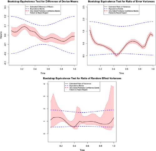
Figure 4: Equivalence Test for the difference of means (top left), ratio of error variances (top right), and the ratio of random effect variance curves (bottom).

5 A frequentist test of equivalence for lung volume functional data

We now conduct our equivalence test using the methods described in Section 4 for paired random effects. We drew 10,000 bootstrap samples and used $\alpha=0.05$ to carry out these tests. We find that Figure 4 is a powerful visual display of the results of this TOST procedure. In each plot, we display the upper and lower equivalence bands. We also display the upper band of the region $C^{l}_{0.95}(\cdot)$ and the lower band of the region $C^{u}_{0.95}(\cdot)$. Recall that we can reject the null if the upper equivalence band lies entirely outside the region $C^{l}_{0.95}(\cdot)$ and if the lower equivalence band lies entirely outside the region $C^{u}_{0.95}(\cdot)$. Hence, it is sufficient to check whether or not either the upper or lower equivalence band at any point intersect the region defined by the overlap of the two one-sided confidence regions, which is shaded in the plots. Intersection implies failure to reject, and lack thereof implies rejection of nonequivalence in favor of equivalence.

Based on Figure 4, we conclude that we can suggest equivalence for our locational metric, but fail to reject the null of nonequivalence for variability of both errors and random effects. We believe it will always be the case that a two-sided test for the variability of random effects is appropriate, as deviations in either direction indicate substantial differences in the distribution of the individual level mean curves; however, for certain applications (ours included), lower error variance will be strictly preferred. If we thus restrict ourselves to only having the ratio of error variances below the upper equivalence threshold, then we would also reject the null of noninferiority of error variability. Note that there does appear to be an inflation of error variance by a factor of 1.5 at the beginning of each breath for SLP relative to spirometry. Though the ratio between the two variances is high at this point, the actual magnitude of the variances at the beginning of these curves is extremely small for both devices, which results in the high value for the ratio of variances.

6 A Bayesian paradigm for equivalence testing

As in the frequentist case, we suggest using functional measures of location and spread to assess practical equivalence, however, carrying out a TOST hypothesis test is not required within the Bayesian paradigm. Rather than conducting a stochastic proof by contradiction, the Bayesian paradigm allows us to directly compute posterior probabilities of our functional metrics of equivalence falling entirely within specified equivalence ranges. That is, the Bayesian paradigm allows for direct computation of $\mathbb{P}\{H_{a}|\mathrm{Data}\}$ for each of the equivalence hypotheses. In light of this, we propose that the researcher conduct the following three steps when using the Bayesian framework for equivalence testing: [3.]

Define an equivalence region through expert consultation.

Define a probability value, call it $\gamma$, such that if $\mathbb{P}\{H_{a}|\mathrm{Data}\}\geq\gamma$, equivalence may be suggested. Using the suggestions of Jeffreys (1961) and Kass and Raftery (1995), a value of $\gamma=0.75$ or $\gamma=0.95$ may be appropriate.

Specify prior distributions for the metrics of equivalence that are commensurate with the researcher’s prior belief of the alternative being true relative to the null.

The specifics of this implementation depend on the types of prior distributions used to model the parameters and data. In Section 7 we discuss the use of Gaussian Processes in modeling both our data and parameters and describe a model that allows for specification of priors and posterior inference for our metrics of equivalence. Though Gaussian Processes are a rich and flexible class of distributions for functional data, a valuable extension of our work would be conducting Bayesian equivalence testing for functional data using nonparametric models.

7 Bayesian functional equivalence testing for lung volume data

Kaufman and Sain (2010) discuss using functional ANOVA modeling within the Bayesian paradigm. They begin by assuming that the functional data are realizations of an underlying Gaussian process with a mean function depending on the factor levels and a covariance function that describes the dependence between points along the function’s domain. They further assume that the covariance between errors can be aptly specified as a member of the class of Matérn covariance functions [Matérn (1986)]. The specification of a correlation function works to impose smoothness between estimated function values and to allow for interpolation at unobserved domain values. Gaussian process priors with Matérn covariance functions are used for the mean functions themselves, which allows for the incorporation of a priori beliefs about both smoothness and location.

The assumption of homoscedastic variances along the function’s domain is problematic for us, as allowing the error and random effect variances to change with time is vital to our investigation of equivalence. We consider a more flexible class of covariance and cross-covariance functions: $\mathbf{V}_{i,j}(t,t^{\prime})=\sigma_{i}(t)\sigma_{j}(t^{\prime})\mathbf{R}_{i,j}(t,t^{\prime})$. Here, $\sigma_{\epsilon,i}(t)$ is the error standard deviation function for device $j$ evaluated at time $t$, and $\mathbf{R}_{\epsilon,i,j}(t,t^{\prime})$ is either the correlation function for device $j$ for observations at times $t$ and $t^{\prime}$ if $i=j$ or the cross-correlation function between the error at time $t$ for device $i$ and the error at time $t^{\prime}$ for device $j$ if $i\neq j$.

To simplify notation, let $\Xi$ denote the set containing all of our parameters. Then, we can write our Multivariate Gaussian Process model for our responses:

$$\left.\left[\begin{array}[]{c}\mathbf{v}_{i,1,k}(\cdot)\\ \mathbf{v}_{i,2,k}(\cdot)\end{array}\right]\right|\Xi\stackrel{{\scriptstyle\mathrm{indep}}}{{\sim}}\operatorname{MVGP}\left(\left[\begin{array}[]{c}\alpha_{i,1}(\cdot)\\ \alpha_{i,2}(\cdot)\end{array}\right],\left[\begin{array}[]{c@{\quad}c}\mathbf{V}_{\epsilon,1,1}(\cdot,\cdot)&\mathbf{V}_{\epsilon,1,2}(\cdot,\cdot)\\ \mathbf{V}_{\epsilon,1,2}(\cdot,\cdot)&\mathbf{V}_{\epsilon,2,2}(\cdot,\cdot)\end{array}\right]\right).$$

Note that, in practice, our response functions are measured only at a predetermined set of grid points, $\mathbf{t}=\{t_{1},\ldots,t_{T}\}\subset\mathcal{T}$. To distinguish this, let the notation $[\mathbf{v}_{i,1,k}(\mathbf{t}),\mathbf{v}_{i,2,k}(\mathbf{t})]$ represent the vector whose coordinates are the response as measured at each of the $T$ grid points, and let the analogous notation hold for the functional parameters of our models. Hence, $[\mathbf{v}_{i,1,k}(\mathbf{t}),\mathbf{v}_{i,2,k}(\mathbf{t})]^{\prime}$ represents a $2T\times 1$ vector. Using the decomposition proposed in Barnard, McCulloch and Meng (2000), our covariance functions evaluated at $\mathbf{t}$ can be described in matrix notation as $\mathbf{V}_{\epsilon,i,j}(\mathbf{t},\mathbf{t})\triangleq\operatorname{Diag}(\sigma_{\epsilon,i}(\mathbf{t}))\mathbf{R}_{\epsilon,i,j}(\mathbf{t},\mathbf{t})\operatorname{Diag}(\sigma_{\epsilon,j}(\mathbf{t}))$, where $\operatorname{Diag}(\sigma_{\epsilon,j}(\mathbf{t}))$ denotes a $T\times T$ matrix whose diagonal elements are $\sigma_{\epsilon,j}(\mathbf{t})$.

Our assumption of a Multivariate Gaussian Process results in $[\mathbf{v}_{i,1,k}(\mathbf{t}),\break\mathbf{v}_{i,2,k}(\mathbf{t})]$ following a Multivariate Normal distribution when we consider observations at the set of gridpoints $\mathbf{t}$ with the fixed grid analogues for the mean and covariance structure.

8 Bayesian methodology

8.1 Correlation structure

Our data set consists of a total of 453 breaths collected from 16 individuals, where each breath was measured at 25 equispaced time points using both SLP and spirometry. Our desire to model cross-covariances between devices results in our matrices of observations being 50 dimensional. For modeling the error correlation, this is not an issue, as we have 453 observations, however, as we only have 16 individuals, a simplifying assumption must be made to proceed. In many functional data settings, the goal of the data analysis is mean function estimation and prediction at new locations (kriging). To facilitate this, modelers typically restrict themselves to a particular class of correlation functions. Unfortunately, the distribution of posterior variance functions is highly dependent on the correlation structure. Hence, misspecification of the correlation model can result in estimates for variance parameters that are biased and wildly misleading. As we would like to conduct inference for the ratio of variance functions of both errors and random effects, we are left searching for an alternative. More advanced methods that make no assumptions on the correlation function class have been suggested in the geostatistics literature [see Nychka, Wikle and Royle (2002), Paciorek and Schervish (2006), Fuentes and Smith (2001), Fuentes (2002)] and elsewhere [see Morris and Carroll (2006), Chen and Müller (2012)], but none of these works have directly focused on the accuracy of the resultant variance estimates. Estimation of correlation functions for repeatedly observed functional data remains an active area of research, particularly in the regime where the number of functional observations is small relative to the grid size.

Our recommendation is that if the researcher has sufficient data to flexibly model the correlation structure of both the random effects and the errors, then this should be the course pursued. As we do not, we instead make a modeling decision that will facilitate valid inference for our variance functions. We assume the following structure for the correlation of our errors and random effects:

$$\mathbf{R}_{i,j}\bigl{(}t,t^{\prime}\bigr{)}=\cases{1,&\quad$i=j,t=t^{\prime}$,\cr\rho(t),&\quad$i\neq j,t=t^{\prime}$,\cr 0,&\quad\mbox{otherwise}.}$$

We thus primarily focus on the marginal distributions for estimation of our mean functions and variances. This has the obvious drawback of not fully exploiting the functional nature of our data, but allows for estimation of marginal variances without the risk of biases due to misspecification of the correlation structure. This is an interesting instance where the simplifying assumptions made to facilitate inference would not necessarily align with ones made if the goal was estimation of mean functions or prediction of values at unmeasured locations. In the latter case, one would likely enforce a restriction to a specific class of correlation functions which would result in both smooth curve estimates and a principled manner by which interpolation and prediction could be performed; however, this would result in misleading estimates for the variance components of the model, which is unacceptable for testing equivalence of variance functions. In Section 10 we investigate the ramifications of this modeling decision on the resultant inference.

8.2 Prior distributions

Specification of priors for $\sigma_{\epsilon,1}(\cdot)$ and $\sigma_{\epsilon,2}(\cdot)$ must be done carefully, as practical equivalence of error variability is tested using a function of these parameters. We model these functions as themselves being realizations of independent stochastic processes. Specifically, we extend the work of Barnard, McCulloch and Meng (2000) to the functional regime by modeling the standard deviation curves as emanating from Log-Gaussian Processes:

$$\log\bigl{(}\sigma^{2}_{\epsilon,1}(\cdot)\bigr{)} \sim \operatorname{GP}\bigl{(}\tau_{\epsilon}(\cdot),s^{2}_{\epsilon}\Gamma_{\epsilon}(\cdot,\cdot)\bigr{)},$$

$$\log\bigl{(}\sigma^{2}_{\epsilon,2}(\cdot)\bigr{)} \sim \operatorname{GP}\bigl{(}\tau^{2}_{\epsilon}(\cdot)-\delta_{\epsilon}(\cdot),s^{2}_{\epsilon}\Gamma_{\epsilon}(\cdot,\cdot)\bigr{)},$$

$$\log\bigl{(}\sigma_{\epsilon,1}(\cdot)\bigr{)} \perp\!\!\!\perp \log\bigl{(}\sigma_{\epsilon,2}(\cdot)\bigr{)},$$

$$p\bigl{(}\tau_{\epsilon}(\cdot)\bigr{)} \propto 1,$$

$$\delta_{\epsilon}(\cdot) \sim \tfrac{1}{2}\mathbh{1}\bigl{\{}\delta_{\epsilon}(\cdot)=\log\bigl{(}\zeta_{l}(\cdot)\bigr{)}\bigr{\}}+\tfrac{1}{2}\mathbh{1}\bigl{\{}\delta_{\epsilon}(\cdot)=\log\bigl{(}\zeta_{u}(\cdot)\bigr{)}\bigr{\}},$$

where ${\Gamma}_{\epsilon}(\cdot,\cdot)=\frac{1}{2}(|t-t^{\prime}|/a_{\epsilon})^{2}\mathcal{K}_{2}(d(t,t^{\prime})/a_{\epsilon})$ is a standard Matérn correlation function [Matérn (1986)] with smoothness parameter $\nu=2$.

We use the ratio $\frac{\sigma^{2}_{\epsilon,1}(\cdot)}{\sigma^{2}_{\epsilon,2}(\cdot)}$ as our comparative measure for the error variability of the two devices. Our prior on the standard deviations yields the following prior for this ratio:

$$\frac{\sigma^{2}_{\epsilon,1}(\cdot)}{\sigma^{2}_{\epsilon,2}(\cdot)} \sim \frac{1}{2}\bigl{(}\mbox{Log-GP}\bigl{(}\log\bigl{(}\zeta_{l}(\cdot)\bigr{)},2s^{2}_{\epsilon}R_{\sigma}(\cdot,\cdot)\bigr{)}\bigr{)}$$

$${}+\frac{1}{2}\bigl{(}\mbox{Log-GP}\bigl{(}\log\bigl{(}\zeta_{u}(\cdot)\bigr{)},2s^{2}_{\epsilon}R_{\sigma}(\cdot,\cdot)\bigr{)}\bigr{)}.$$

This is a $50/50$ mixture of two Log-Gaussian Processes with medians at the upper and lower equivalence thresholds respectively. Hence, we can place prior probabilities on falling within the equivalence region by careful choices of $s^{2}_{\epsilon}\Gamma_{\epsilon}(\cdot,\cdot)$. Borrowing from the frequentist paradigm in which it is incumbent upon the researcher to prove his or her hypothesis beyond a reasonable doubt, we set the values of these hyperparameters such that the a priori probability of equivalence is quite small. We set $s_{\epsilon}^{2}=5$ and $a_{\epsilon}=0.1$, which results in a prior probability of falling entirely within the equivalence region of $\mathbb{P}\{\sigma^{2}_{\epsilon,1}(\mathbf{t})/\sigma^{2}_{\epsilon,2}(\mathbf{t})\in(\zeta_{l}(\mathbf{t}),\zeta_{u}(\mathbf{t}))\}\approx 5\times 10^{-8}$.

For the correlations resulting from the paired nature of our data, we set $\rho_{\epsilon}(t)\sim\mathcal{U}[-1,1]$ for all $t$.

For our random effects, $\{[\alpha_{i,1}(\cdot),\alpha_{i,2}(\cdot)]\}$, we use a Hierarchical Gaussian Process prior:

$$\left[\begin{array}[]{c}\alpha_{i,1}(\cdot)\\ \alpha_{i,2}(\cdot)\end{array}\right]\stackrel{{\scriptstyle\mathrm{i.i.d.}}}{{\sim}}\operatorname{GP}\left(\left[\begin{array}[]{c}\mu_{1}(\cdot)\\ \mu_{2}(\cdot)\end{array}\right],\left[\begin{array}[]{c@{\quad}c}\mathbf{V}_{\alpha,1,1}(\cdot,\cdot)&\mathbf{V}_{\alpha,1,2}(\cdot,\cdot)\\ \mathbf{V}_{\alpha,1,2}(\cdot,\cdot)&\mathbf{V}_{\alpha,2,2}(\cdot,\cdot)\end{array}\right]\right).$$

The priors on the variance functions of our random effects, $[\sigma^{2}_{\alpha,1}(\cdot),\sigma^{2}_{\alpha,2}(\cdot)]$, and the correlation structure are identical to the one used for the error variances.

The posterior distribution for the difference between the device specific curves, $\mu_{1}(\cdot)-\mu_{2}(\cdot)$, is of interest for assessing locational equivalence. Thus, proper attention must be paid to the prior placed on $\{\mu_{1}(\cdot),\mu_{2}(\cdot)\}$ such that the prior does not unduly force the posterior distribution toward the prespecified equivalence region. Our priors for $\mu_{1}(\cdot)$ and $\mu_{2}(\cdot)$ are as follows:

$$\mu_{1}(\cdot) \sim \operatorname{GP}\bigl{(}\mu_{0}(\cdot),s^{2}_{\mu}\Gamma_{\mu}(\cdot,\cdot)\bigr{)},$$

$$\mu_{2}(\cdot) \sim \operatorname{GP}\bigl{(}\mu_{0}(\cdot)-\delta_{\mu}(\cdot),s^{2}_{\mu}\Gamma_{\mu}(\cdot,\cdot)\bigr{)},$$

$$\mu_{1}(\cdot) \perp\!\!\!\perp \mu_{2}(\cdot),$$

$$p\bigl{(}\mu_{0}(\cdot)\bigr{)} \propto 1,$$

$$\delta_{\mu}(\cdot) \sim \tfrac{1}{2}\mathbh{1}\bigl{\{}\delta_{\mu}(\cdot)=\kappa_{l}(\cdot)\bigr{\}}+\tfrac{1}{2}\mathbh{1}\bigl{\{}\delta_{\mu}(\cdot)=\kappa_{u}(\cdot)\bigr{\}},$$

where $\Gamma_{\mu}(t,t^{\prime})$ is a Matérn correlation function with smoothness parameter $\nu=2$. This then implies that our difference of means has the following prior:

$$\mu_{1}(\cdot)-\mu_{2}(\cdot)\sim\tfrac{1}{2}\bigl{(}\operatorname{GP}\bigl{(}\kappa_{l}(\cdot),2s^{2}_{\mu}\Gamma_{\mu}(\cdot,\cdot)\bigr{)}\bigr{)}+\tfrac{1}{2}\bigl{(}\operatorname{GP}\bigl{(}\kappa_{u}(\cdot),2s^{2}_{\mu}\Gamma_{\mu}(\cdot,\cdot)\bigr{)}\bigr{)}.$$

In other words, our prior on the difference in device means is a $50/50$ mixture of two Gaussian Processes, with means at the upper and lower equivalence thresholds respectively. We choose a prior that places 1% likelihood in the equivalence region and the remaining 99% outside of it. To achieve this, we fixed a value of $a_{\mu}=0.3$, and then used the uniroot() and pmvnorm() functions in R [R Development Core Team (2011)] to solve for the value of $s^{2}_{\mu}$ such that $\mathbb{P}\{\mu_{1}(\mathbf{t})-\mu_{2}(\mathbf{t})\in(\kappa_{l}(\mathbf{t}),\kappa_{u}(\mathbf{t}))\}=0.01$. This value was found to be 0.1. Note that if one has a sense of an appropriate basis for the mean functions, one could place a prior $\mu_{0}(\cdot)\sim\mathcal{N}(\sum a_{k}\phi_{k}(\cdot),\sigma^{2}_{\mu})$ instead of $p(\mu_{0}(\cdot))\propto 1$. This could allow for regularization of the functional fits based on this basis while not restricting them to entirely follow said basis, and would still facilitate our strategy of putting priors on equivalence commensurate with prior knowledge.

8.3 Posterior sampling

Before conducting inference based on our model specification, we must devise a sampling schema for the posterior distribution of our parameters. We use a Metropolis-within-Gibbs sampling algorithm; see the supplementary materials [Fogarty and Small (2014)] for details.

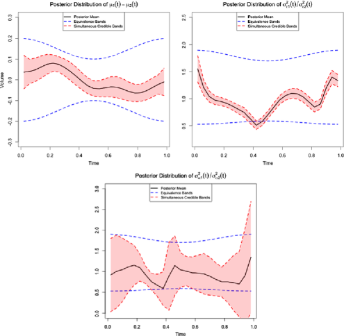
Figure 5: 95% simultaneous credible bands for $\mu_{1}(\cdot)-\mu_{2}(\cdot)$ (top left), $\sigma^{2}_{\epsilon,1}(\cdot)/\sigma^{2}_{\epsilon,2}(\cdot)$ (top right), and $\sigma^{2}_{\alpha,1}(\cdot)/\sigma^{2}_{\alpha,2}(\cdot)$ (bottom), along with upper and lower equivalence bands.

9 Posterior analysis

To conduct our posterior analysis, we ran our Gibbs sampler from three distinct starting values for 10,500 iterations per starting value (for a total of 31,500 iterations). We discarded the first 500 iterations as burn-in for each chain and took every 10 samples thenceforth for a total of 1000 samples per starting value, which were then chained together, resulting in 3000 roughly independent samples. See the supplementary material [Fogarty and Small (2014)] for convergence diagnostics.

Figure 5 shows the posterior distribution for the three metrics of interest. We summarize the posterior distributions of our metrics of equivalence by the posterior mean curve and 95% simultaneous posterior bands. These bands are computed using the multiplier based method of Buja and Rolke (2003). The posterior bands are unnecessary for inference, as the computation of $\mathbb{P}\{H_{a}|\mathrm{Data}\}$ depends solely on how many posterior curves fall within the equivalence region, but nonetheless provide a useful graphical aid. For our locational metric, $\mu_{1}(\cdot)-\mu_{2}(\cdot)$, we found that all 3000 of our samples from the posterior distribution fell within the prespecified equivalence range, suggesting overwhelming evidence in favor of the hypothesis that these two curves, in terms of location, can be considered practically equivalent. For the ratio of error variances, $\sigma^{2}_{\epsilon,1}(\cdot)/\sigma^{2}_{\epsilon,2}(\cdot)$, we note that if it is the case that lower variability is strictly more desirable, then 2998 out of 3000 samples fall strictly below the upper equivalence band; however, if one desires adherence to the lower equivalence band as well, then our posterior probability of equivalence is $0.0007$, since our posterior bands regularly violate the lower tolerance threshold toward the middle of the breaths (around $t=0.5$). For the ratio of random effect variances, $\sigma^{2}_{\alpha,1}(\cdot)/\sigma^{2}_{\alpha,2}(\cdot)$, we note that although the posterior median falls well within the equivalence range, only 18.2% of the posterior samples fell entirely within the equivalence region. Hence, although we can suggest equivalence of both means and error variances, we lack sufficient power to suggest equivalence of random effect variances.

10 Comparing the frequentist and Bayesian methods

We have presented methods for equivalence testing within the frequentist and Bayesian paradigms. From a pragmatic perspective, the relative computational intensity of both methods is of interest to practitioners. In this respect, our frequentist method is dominant, as within each bootstrap iteration, only simple vector operations are required. The Bayesian approach requires sampling from multivariate distributions, matrix multiplication, matrix inversion, and determinant calculation within each step. Furthermore, thinning of one out of every 10 iterations was required. Hence, to get the same effective sample size, we needed to do 10 times as many iterations for the frequentist procedure as we did for the Bayesian one. To attain 1000 independent samples via the Bayesian methodology, we needed to run 10,500 iterations of our sampling algorithm, which took 22.6 minutes on a personal laptop with 4 GB RAM and a 2.7 GHz processor. The bootstrap procedure took 16.1 seconds to run 1000 iterations on the same laptop. This discrepancy will only increase as the granularity of the grid the user implements increases, as both determinant and inverse calculation are $O(p^{3})$ in their simplest implementation.

Frequentist and Bayesian inference are not coherent with one another, in that frequentist inference has a built in preference for the null hypothesis. For the frequentist, the null is the status quo, and the goal of the inference is to refute it via a “proof by contradiction.” The Bayesian framework, on the other hand, allows the user to put varying degrees of a priori preference on one hypothesis versus the other. In our Bayesian analysis we have placed heavy preference on the null and thus require very strong evidence from the data to put the posterior probability in the proper region, but this may not always be appropriate. The Bayesian paradigm allows for a principled manner for incorporating the results of past studies in the form of the priors placed on equivalence vs nonequivalence, a feature not offered by the frequentist framework.

With these caveats in mind, we investigate the size and power of our methodologies, using the threshold of $\alpha=0.05$ in the frequentist procedure. For our Bayesian procedure, we use $\gamma=0.95$ as our threshold for the posterior probability of equivalence. In our investigation, we continue to place heavy a priori preference on nonequivalence for our Bayesian methodology.

10.1 Type I error

We restrict our investigation to the Type I error rates of our tests for location and error variances. We simulate 20 matched pair random effects, and then simulate 20 matched functional responses for each subpopulation. This results in 400 breaths total. To investigate the true size of our methods, we define a sequence of true values for our metrics of equivalence where equivalence is violated at one point along the domain, and the other points move farther and farther into the equivalence region. These sequences and numerical labels are shown in Figure 6. The remaining values of parameters needed for simulation are based on the posterior means from our data set. Additionally, we used an estimate of the correlation structure of our error functions as the true correlation for simulating both error functions and random effect functions. This allows us to assess the robustness of our Bayesian procedure to the assumption of Section 8.1

For each of the nine function values in the sequence, we simulated 500 data sets and ran both the frequentist and Bayesian methdologies on them. Figure 6 shows the result of this study. We see that for testing the equivalence of mean functions, the Bayesian procedure is far more conservative than our frequentist procedure, which appears to be due to the assumption on the correlation structure made in our Bayesian procedure. As expected, the frequentist procedure is initially conservative, but has size that approaches 0.05 as the test becomes increasingly reliant on our data’s behavior at one domain point (the one at which equivalence is violated). Figure 6 also demonstrates that the test is roughly unbiased in terms of purported size. For testing the equivalence of variances, the Bayesian and frequentist procedures initially exhibit similar Type I error rates, and also both appear to be slighty anti-conservative; however, the Bayesian procedure is anti-conservative to a far more egregious degree by the end of the sequence of functions, having an estimated size of 0.072 for the 9th function in the sequence versus an estimated size of 0.056 for the frequentist procedure at this value for the true ratio of error variances.

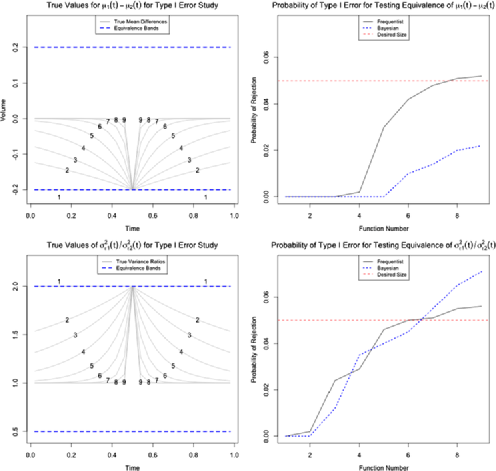
Figure 6: Sequence of true values and corresponding Type I error rates for $\mu_{1}(\cdot)-\mu_{2}(\cdot)$ (top) and $\sigma^{2}_{\epsilon,1}(\cdot)/\sigma^{2}_{\epsilon,2}(\cdot)$ (bottom) along with upper and lower equivalence bands used for Type I error study.

10.2 Power

To investigate the power of our methods, we define a sequence of true values for our metrics of equivalence that fall entirely between the upper and lower equivalence thresholds. These sequences and numerical labels are shown in Figure 7. The rest of our simulation procedure mirrors that of our simulation for testing the Type I error rate. Figure 7 shows the results of this study. We see that for testing equivalence of means, the frequentist procedure appears to be substantially more powerful than its Bayesian counterpart. For testing equivalence of variances, the frequentist and Bayesian procedures behave quite similarly, with no clear indication that one procedure is any more powerful than the other.

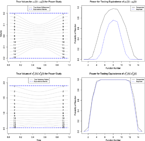
Figure 7: Sequence of true values and corresponding power of $\mu_{1}(\cdot)-\mu_{2}(\cdot)$ (top) and $\sigma^{2}_{\epsilon,1}(\cdot)/\sigma^{2}_{\epsilon,2}(\cdot)$ (bottom) along with upper and lower equivalence bands used for the power study.

11 Discussion

We have presented a broad framework for equivalence testing when one’s data are intrinsically functional. This framework begins with definitions of metrics of equivalence, and correspondingly with the establishment of upper and lower equivalence bands which are themselves functions of the continuum over which the functional data is defined. We have stressed the importance of using metrics that are able to discern similarity of location and of spread, as neither individually is sufficient for suggesting equivalence. We illustrated the proper use of these frameworks using data from a method comparison study assessing the performance of a new device for testing pulmonary function, SLP, relative to the gold standard for pulmonary diagnoses, the spirometer.

Our model presently makes an assumption that all individuals are drawn from the same population. For our application this makes sense, as we are solely looking at healthy individuals. For other applications, the individuals for which repeated measurements are attained may be draws from multiple populations. In our application, one could potentially have individuals of varying degrees of pulmonary health (e.g., healthy, asthmatic, smokers). Our model can easily adapt to this, as this simply requires adding an additional level to the hierarchy. We could either say that health level specific means are drawn from a population with an overall mean, and then individual means are drawn from these health level specific populations, or we could model the health level means as fixed effects and result in a functional mixed effects model.

Using the difference between mean functions to test locational disparity is a natural choice, and the extent to which magnitude of differences are important can be controlled by tightening or loosening the equivalence bands. For testing the disparity between variances of both errors and random effects, we have followed the prevalent choice in the scalar equivalence testing literature [see Chow and Liu (1992)] and have used the ratio between variances, $\sigma^{2}_{1}(\cdot)/\sigma^{2}_{2}(\cdot)$. On the one hand, this unitless measure has appeal in that it has potential for standardization across applications. On the other hand, we lose a sense of the absolute difference between the quantities. For some applications, the difference between a variance of 0.01 and 0.02 could be inconsequential, yet the difference between 0.04 and 0.08 could be enough to warrant using one device over another. If one were using ratios for assessing a discrepancy, however, these quantities would be identically different. We thus suggest that the difference between variances, $\sigma^{2}_{1}(\cdot)-\sigma^{2}_{1}(\cdot)$, may be an additional metric for equivalence that could be used in tandem with the ratio of variances to test for equivalence of variability.

Note that there may be additional facets of the underlying distributions of functions to be addressed beyond location and variability, depending on the application. For example, one may be interested not only in the difference in the mean functions being within an equivalence region, but also in the derivative of the difference between mean functions being small in absolute value. We leave the development of proper methodology for these questions as a topic for future research, but the strategy of supplying upper and lower equivalence bands would certainly be appropriate.

We hope that this paper serves as a valuable contribution to the literature on equivalence testing and that its extension to the realm of functional data will be useful for a host of applied users, including but not limited to practitioners looking to compare devices whose measurements cannot be summarized as scalar quantities. Comparison studies are of the utmost importance, as oftentimes the emergence of newer and better devices can have salubrious outcomes for society in general. Our goal is that this paper properly emphasizes the importance of equivalence testing in general, and provides traction for researchers who aim to suggest that two populations of functions are practically equivalent rather than to suggest that they are different.