Rarefaction acceleration in magnetized gamma-ray burst jets

Abstract

Relativistic jets associated with long/soft gamma-ray bursts are formed and initially propagate in the interior of the progenitor star. Because of the subsequent loss of their external pressure support after they cross the stellar surface, these flows can be modeled as moving around a corner. A strong steady-state rarefaction wave is formed, and the sideways expansion is accompanied by a rarefaction acceleration. We investigate the efficiency and the general characteristics of this mechanism by integrating the steady-state, special relativistic, magnetohydrodynamic equations, using a special set of partial exact solutions in planar geometry ($r$ self-similar with respect to the “corner”). We also derive analytical approximate scalings in the ultrarelativistic cold/magnetized, and hydrodynamic limits. The mechanism is more effective in magnetized than in purely hydrodynamic flows. It substantially increases the Lorentz factor without much affecting the opening of the jet; the resulting values of their product can be much grater than unity, allowing for possible breaks in the afterglow light curves. These findings are similar to the ones from numerical simulations of axisymmetric jets by Komissarov et al and Tchekhovskoy et al, although in our approach we describe the rarefaction as a steady-state simple wave and self-consistently calculate the opening of the jet that corresponds to zero external pressure.

1 Introduction

The commonly accepted paradigm for gamma-ray bursts (GRBs) is that they are formed in ultrarelativistic, collimated jets. Typical terminal Lorentz factors for these jets, such that the photons can freely escape, are $\Gamma_{j}\sim$ a few hundreds, even above on thousand (e.g. Lithwick & Sari, 2001; Zhao et al., 2011). Opening angles $\Theta_{j}$ are inferred from achromatic breaks in the afterglow light curves, although these are not clearly detected in several bursts (e.g., Liang et al., 2008; Racusin et al., 2009; Cenko et al., 2010). Since the Lorentz factor decreases during the afterglow phase, and the break in the light curves occurs when the beaming angle equals $\Theta_{j}$, the product $\Gamma_{j}\Theta_{j}$ should be larger than one at the start of this phase, typically of the order of a few tens.

The long/soft class of GRBs are thought to be connected with the death of massive stars, since some of them are associated with Type Ic supernovae and are observed in star-forming regions of the host galaxies (see e.g., Zhang, 2011 and references therein). During this process a compact central object and accretion disk are formed, and the jet is powered by either the neutrino annihilation, or by magnetic fields, tapping the rotational energy of the central object or disk. It is not clear which of the two mechanisms (or both) operates, with the detection or not of the thermal photospheric emission being a key factor (Zhang & Pe’er, 2009; Pe’er et al., 2012).

Thermal (fireball) acceleration is in general a fast and efficient process, with the Lorentz factor increasing linearly with the cylindrical distance from the symmetry axis. Magnetic acceleration also works provided that the jet is supported externally by an environment whose pressure does not drop faster than the inverse square of the distance from the origin, as was analytically shown in (Komissarov et al., 2009). The interior of the progenitor star could very well play this role. Relativistic magnetohydrodynamic (MHD) simulations by (Komissarov et al., 2009) show that the efficiency of the magnetic acceleration is $\sim 50\%$ or more. The model faces two problems though: (1) The jet looses its external support when it exits the progenitor star, its motion becomes ballistic and its acceleration is practically halted. (2) The magnetic acceleration requires that the flow is expanded in a way such that the separation between neighboring streamlines increases faster than the cylindrical radius. This is achieved through stronger collimation of the inner part of the outflow relative to the outer part, and for this reason the mechanism was dubbed collimation-acceleration by Komissarov et al. (2009). The resulting jets are very narrow with $\Theta_{j}\sim 1/\Gamma_{j}$, and the product $\Gamma_{j}\Theta_{j}$ is close to unity before the start of the afterglow phase, making the breaks unlikely to happen.

A solution to both problems can be given by carefully studying the dynamics at the regime where the jet comes out from the star, and its external pressure drops to practically zero. Tchekhovskoy et al. (2010) simulated this transition and found that it is accompanied by a spurt of acceleration. Komissarov et al. (2010) confirmed their finding numerically and interpreted it as rarefaction acceleration. The loss of external support induces a sideways expansion of the jet, and a strong rarefaction wave that is driven into the flow and accelerates it.

In fact this is a powerful mechanism seen in other numerical simulations of both, hydrodynamic and MHD flows with contact discontinuity and flow along it, see Aloy & Rezzolla (2006); Mizuno et al. (2008); Zenitani et al. (2010); Matsumoto et al. (2012).
A similar mechanism was studied in Lyutikov, 2011; Granot et al., 2011, for the problem of an initially static magnetized plasma allowing to move into an environment. Here we are interested for non-static cases and their sideways expansion.

However, the analysis in all these works were based on time dependent simple waves, while for the GRB problem under consideration it is more appropriate to use steady-state simple waves. In the present paper we develop a model for the steady-state, relativistic, magnetized, rarefaction wave.

The work is a generalization of the classical steady-state, hydrodynamic rarefaction analyzed in Landau & Lifschitz (1987), and its relativistic (but again unmagnetized) counterpart by Granik (1982); Kolosnitsyn & Stanyukovich (1984).

In Section 2 we review the steady-state, special relativistic, MHD equations in planar geometry. In Section 3 we develop the model, in Section 4 we present and discuss the results and their application to GRBs. Finally, in Section 5 we give a summary.

2 Basic equations

The system of equations of special relativistic, ideal MHD, consist of the Ohm’s law

$${\mn@boldsymbol{E}}=-\frac{\mn@boldsymbol{v}}{c}\times\mn@boldsymbol{B}\,,$$ (1)

the Maxwell equations

$$\nabla\cdot\mn@boldsymbol{B}=0\,,\quad\nabla\times\mn@boldsymbol{E}=-\frac{1}{c}\frac{\partial\mn@boldsymbol{B}}{\partial t}\,,$$ (2)

the mass

$$\frac{\partial\left(\Gamma\rho\right)}{\partial t}+\nabla\cdot\left(\Gamma\rho\mn@boldsymbol{v}\right)=0\,,$$ (3)

momentum

$$\Gamma\rho\left(\frac{\partial}{\partial t}+{\mn@boldsymbol{v}}\cdot\nabla\right)\left(h\Gamma{\mn@boldsymbol{v}}\right)=-\nabla p+\qquad$$

$$\frac{\nabla\cdot\mn@boldsymbol{E}}{4\pi}\mn@boldsymbol{E}+\left(\frac{\nabla\times\mn@boldsymbol{B}}{4\pi}-\frac{1}{4\pi c}\frac{\partial\mn@boldsymbol{E}}{\partial t}\right)\times\mn@boldsymbol{B}\,,$$ (4)

and entropy

$$\left(\frac{\partial}{\partial t}+\mn@boldsymbol{v}\cdot\nabla\right)p=\rho c^{2}\left(\frac{\partial}{\partial t}+\mn@boldsymbol{v}\cdot\nabla\right)h$$ (5)

conservation equations (e.g., Vlahakis & Königl, 2003).
Here $\mn@boldsymbol{v}$ is the velocity of the outflow, $\Gamma$ is the associated Lorentz factor satisfying

$$\Gamma^{2}=1+\left(\Gamma\mn@boldsymbol{v}/c\right)^{2}\,,$$ (6)

$(\mn@boldsymbol{E}\,,\mn@boldsymbol{B})$ the electromagnetic field as measured in the central object’s frame, $\rho$ the rest mass density, $p$ the gas pressure, and $h=w/\rho c^{2}$ the specific enthalpy (over $c^{2}$), whose expression is, for an ideal gas with polytropic index $\gamma$,

$$h=1+\frac{\gamma}{\gamma-1}\frac{p}{\rho c^{2}}\,.$$ (7)

The polytropic index takes the values $4/3$ or $5/3$ in the limit of ultrarelativistic or nonrelativistic temperatures, respectively. (Any other value would imply a nonadiabatic evolution and hence requires the incorporation of heating/cooling terms into the entropy and momentum equations. See also Chiu, 1973 for intermediate temperatures.)

By assuming steady state ($\partial/\partial t=0$) and a planar symmetric flow, i.e., $\partial/\partial y=0$ in a system of Cartesian spatial coordinates $\left(x,y,z\right)$, we can carry out a partial integration of the above equations (1–7). It is also sufficient to simplify the analysis by assuming that the flow lies on the poloidal plane $x-z$, $v_{y}=0$, and the magnetic field in the transverse direction, $\mn@boldsymbol{B}=B\hat{y}$. As discussed in Section 4, these are reasonable assumptions when the model is applied to GRB outflows. It is possible to generalize the analysis to planar symmetric magnetized flows with nonzero $v_{y}$ and poloidal magnetic field; this will be presented in a future paper.

The continuity equation (3) for steady flows on the $x-z$ plane yields $\Gamma\rho\mn@boldsymbol{v}=\nabla\times\left[\Psi(x,z)\hat{y}\right]$, and thus the flow velocity can be expressed as

$$\mn@boldsymbol{v}=\frac{1}{\Gamma\rho}\nabla\Psi\times\hat{y}\,.$$ (8)

The stream function $\Psi$ is constant along each streamline (since $\mn@boldsymbol{v}\cdot\nabla\Psi=0$), and can be used as its “label”.

Using Ohm’s equation (1) we express the electric field as $\mn@boldsymbol{E}=\left({B}/{\Gamma\rho c}\right)\nabla\Psi$. Substituting in Faraday’s equation (2) we find $\nabla\left(B/\Gamma\rho c\right)\times\nabla\Psi=0$, which means that the quantity $B/\Gamma\rho c$ is a streamline constant,

$$-\frac{B}{\Gamma\rho c}=\Phi_{\Psi}(\Psi)\,.$$ (9)

Thus, the electric field can be written as $\mn@boldsymbol{E}=-\Phi_{\Psi}\nabla\Psi=-\nabla\int\Phi_{\Psi}d\Psi$. This expression shows the relation of the function $\Phi_{\Psi}$ with the scalar electric potential, and also that the streamlines are equipotentials.

The component of the momentum equation (2) along the flow gives after some manipulation

$$h\Gamma-\frac{\Phi_{\Psi}B}{4\pi c}=\mu(\Psi)\,.$$ (10)

This integral represents the total energy-to-mass flux ratio (over $c^{2}$), since the mass flux (times $c^{2}$) is $c^{2}\Gamma\rho\mn@boldsymbol{v}$, the Poynting flux $(c/4\pi)\mn@boldsymbol{E}\times\mn@boldsymbol{B}=-({\Phi_{\Psi}B}/{4\pi c})c^{2}\Gamma\rho\mn@boldsymbol{v}$, and the matter energy flux (including thermal, bulk kinetic and rest energy) is $c^{2}\Gamma^{2}h\rho\mn@boldsymbol{v}$.

The entropy conservation equation (5), for an ideal gas whose enthalpy is given by equation (7), simplifies to $\mn@boldsymbol{v}\cdot\nabla(p/\rho^{\gamma})=0$, meaning that the quantity $p/\rho^{\gamma}$ – which is related to the specific entropy – is a streamline constant

$$\frac{p}{\rho^{\gamma}}=Q(\Psi)\,.$$ (11)

The previous partial integrations greatly simplify the original system of equations (1)–(7), yielding several streamline constants, which can be determined at the boundary of the flow. Three equations remain to be integrated: the component of the momentum equation (2) normal to the flow velocity, and equations (6), (7). There are correspondingly three unknown functions, which we choose to be the stream function $\Psi$, the specific enthalpy $h$, and the ratio of Poynting-to-matter energy flux

$$\sigma\equiv\frac{B^{2}}{4\pi h\Gamma^{2}\rho c^{2}}=\frac{\Phi_{\Psi}^{2}\rho}{4\pi h}\,.$$ (12)

We may write the physical quantities in terms of these variables:

$$\rho=\frac{4\pi h\sigma}{\Phi_{\Psi}^{2}}\,,\quad p=Q\rho^{\gamma}\,,$$ (13)

$$\Gamma=\frac{\mu}{h\left(1+\sigma\right)}\,,\quad\mn@boldsymbol{v}=\frac{\nabla\Psi\times\hat{y}}{\Gamma\rho}\,,$$ (14)

$${\mn@boldsymbol{B}}=-\frac{4\pi\mu c}{\Phi_{\Psi}}\frac{\sigma}{1+\sigma}\hat{y}\,,\quad{\mn@boldsymbol{E}}=-\Phi_{\Psi}\nabla\Psi\,.$$ (15)

Knowing the streamline constants ($\Phi_{\Psi}$, $\mu$, $Q$) we can find the remaining unknowns $\Psi\,,\sigma\,,h$ by solving the following system of equations, with the first coming from equation (7), the second from equation (6), and the third from the component of the momentum equation (2) normal to the flow velocity:

$$h=1+\frac{\gamma}{\gamma-1}\frac{Q}{c^{2}}\left(\frac{4\pi}{\Phi_{\Psi}^{2}}\right)^{\gamma-1}(h\sigma)^{\gamma-1}\,,$$ (16)

$$\frac{\mu^{2}}{h^{2}(1+\sigma)^{2}}=1+\left(\frac{\Phi_{\Psi}^{2}\nabla\Psi}{4\pi ch\sigma}\right)^{2}\,,$$ (17)

$$\frac{\Phi_{\Psi}^{2}}{\sigma}\left[\left(1+\sigma\right)\nabla^{2}\Psi-\nabla\Psi\cdot\nabla\ln\mid\nabla\Psi\mid\right]$$

$$-\frac{1}{2}\nabla\left(\frac{4\pi\mu c}{\Phi_{\Psi}}\frac{\sigma}{1+\sigma}\right)^{2}\cdot\frac{\nabla\Psi}{\mid\nabla\Psi\mid^{2}}+\frac{\mid\nabla\Psi\mid^{2}}{2}\frac{d\Phi_{\Psi}^{2}}{d\Psi}$$

$$-\frac{\gamma-1}{\gamma}\nabla\left[16\pi^{2}c^{2}\frac{h(h-1)\sigma}{\Phi_{\Psi}^{2}}\right]\cdot\frac{\nabla\Psi}{\mid\nabla\Psi\mid^{2}}=0\,.$$ (18)

3 The $r$ self-similar model

The problem under consideration is basically a Prandtl-Meyer flow around a corner, and thus the appropriate coordinates are polar on the plane $x-z$ with the corner at the origin, defined through $x=r\sin\theta$ and $z=r\cos\theta$, see Fig. 1. A self-similar flow is described with a stream function of the form $\Psi=r^{\lambda}\psi(\theta)$, with constant $\lambda$. It is more convenient to replace the function $\psi(\theta)$ in terms of the function $f(\theta)$, defined through $\psi=\Psi_{0}(r_{0}f)^{-\lambda}$, with constant $\Psi_{0}$, $r_{0}$, in which case the definition of $\Psi$ yields

$$r=r_{\Psi}f(\theta)\,,\quad r_{\Psi}\equiv r_{0}\left(\frac{\Psi}{\Psi_{0}}\right)^{1/\lambda}\,.$$ (19)

The function $f(\theta)$ gives the radial distance from the corner, modulo a scale factor which is different in each streamline. This clearly shows that all streamlines are similar to each-other, hence the term “self-similarity”.

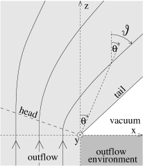
Figure 1: The outflow geometry.

The derivative of $f(\theta)$ controls $\nabla\Psi$, and is thus related to the flow direction. Rewriting equation (14) as $\Gamma\rho\mn@boldsymbol{v}=\displaystyle\frac{1}{r}\frac{\partial\Psi}{\partial\theta}\hat{r}-\displaystyle\frac{\partial\Psi}{\partial r}\hat{\theta}$, where $\hat{r}$ and $\hat{\theta}$ the unit vectors of the polar coordinates, and defining the angle $\vartheta$ between the flow velocity and the $z$ axis (see Fig. 1), the $\tan\left(\vartheta-\theta\right)=v_{\theta}/v_{r}$ yields

$$\frac{df}{d\theta}=\frac{f}{\tan\left(\vartheta-\theta\right)}\,.$$ (20)

Our goal is to separate the variables $r$ and $\theta$ in the system of equations (16)–(2), and reduce them to equations with respect to the polar angle $\theta$ alone.

From inspection of equations (16), (17) we require

$$\sigma=\sigma(\theta)\,,\quad h=h(\theta)\,,\mbox{ and constant }\mu\,,\ Q/\Phi_{\Psi}^{2(\gamma-1)}\,.$$ (21)

The last term of equation (17) should be a function of $\theta$ alone, and this gives the form of the streamline constant

$$\Phi_{\Psi}^{2}=\frac{4\pi cr_{0}}{\lambda\mid\Psi_{0}\mid}\left(\frac{\Psi}{\Psi_{0}}\right)^{\frac{1}{\lambda}-1}\,.$$ (22)

The so-called Bernoulli equation (17) can then be written as

$$\frac{\mu^{2}}{h^{2}(1+\sigma)^{2}}=1+\frac{1}{h^{2}\sigma^{2}f^{2}\sin^{2}\left(\vartheta-\theta\right)}\,,$$ (23)

or in differential form

$$\frac{d\vartheta}{d\theta}=-\frac{\tan\left(\vartheta-\theta\right)\left[\mu^{2}-h^{2}(1+u_{s}^{2})\left(1+\sigma\right)^{3}\right]}{\sigma\left(1+\sigma\right)\left[\mu^{2}-h^{2}\left(1+\sigma\right)^{2}\right]}\frac{d\sigma}{d\theta}\,,$$ (24)

where we used the differential form of equation (16)

$$\frac{dh}{d\theta}=\frac{hu_{s}^{2}}{\sigma}\frac{d\sigma}{d\theta}\,,\quad u_{s}^{2}=\frac{\left(\gamma-1\right)\left(h-1\right)}{\gamma-1+\left(2-\gamma\right)h}\,.$$ (25)

$u_{s}^{2}$ is the square of the proper sound speed (over $c^{2}$)

$$u_{s}^{2}=\frac{c_{s}^{2}/c^{2}}{1-c_{s}^{2}/c^{2}}\,,\quad c_{s}^{2}=\frac{\gamma p}{\rho h}\,.$$ (26)

The transfield equation (2), after some manipulation using the previous two equations, gives

$$\frac{d\sigma}{d\theta}=-\frac{\left(\lambda-1\right)\sigma}{2\tan\left(\vartheta-\theta\right)}\frac{{\cal N}}{{\cal D}}\,,$$ (27)

$${\cal N}=\sigma+\frac{2}{\gamma}\frac{u_{s}^{2}}{1+u_{s}^{2}}\,,\quad{\cal D}=\frac{1}{h^{2}\sigma^{2}f^{2}}-\sigma\left(1+u_{s}^{2}\right)-u_{s}^{2}\,.$$

After solving the system of equations (16), (20), (23), (27) for the functions $f(\theta)$, $\vartheta(\theta)$, $h(\theta)$, $\sigma(\theta)$, the physical quantities can be recovered using

$$\rho=\frac{\lambda|\Psi_{0}|}{cr_{0}}h\sigma\left(\frac{r}{r_{0}f}\right)^{\lambda-1}\!\!,\quad\frac{p}{\rho c^{2}}=\frac{\left(\gamma-1\right)\left(h-1\right)}{\gamma}\,,$$ (28)

$$\Gamma\frac{\mn@boldsymbol{v}}{c}=-\frac{\Psi_{0}}{|\Psi_{0}|}\frac{\cos\left(\vartheta-\theta\right)\hat{r}+\sin\left(\vartheta-\theta\right)\hat{\theta}}{hf\sigma\sin\left(\vartheta-\theta\right)}\,,$$ (29)

$$\Gamma=\frac{\mu}{h\left(1+\sigma\right)}\,,\quad\frac{\mn@boldsymbol{B}}{\sqrt{4\pi\rho hc^{2}}}=-\frac{\Phi_{\Psi}}{|\Phi_{\Psi}|}\frac{\mu\ \sigma^{1/2}}{h(1+\sigma)}\hat{y}\,,$$ (30)

$$\frac{\mn@boldsymbol{E}}{\sqrt{4\pi\rho hc^{2}}}=-\frac{\Psi_{0}}{|\Psi_{0}|}\frac{\Phi_{\Psi}}{|\Phi_{\Psi}|}\frac{\sin\left(\vartheta-\theta\right)\hat{r}-\cos\left(\vartheta-\theta\right)\hat{\theta}}{hf\sigma^{1/2}\sin\left(\vartheta-\theta\right)}\,.$$ (31)

Note that, using the previous expressions, the numerator and denominator of the differential equation (27) can be written as

$${\cal N}=\frac{B^{2}-E^{2}}{4\pi\rho hc^{2}}+\frac{2}{\gamma}\frac{u_{s}^{2}}{1+u_{s}^{2}}\,,$$

$${\cal D}=\left(\frac{\Gamma v_{\theta}}{c}\right)^{2}-{\displaystyle\frac{B^{2}-E^{2}}{4\pi h\rho c^{2}}(1+u_{s}^{2})-u_{s}^{2}}\,.$$ (32)

${\cal N}$ is always positive, while ${\cal D}$ can be written as $(\Gamma v_{\theta}/c)^{2}-u_{\rm f}^{2}$ (using expression 38 of Appendix A).

3.1 The rarefaction wave $(\lambda=1)$ case

Near the corner the flow properties are expected to depend mostly on the polar angle $\theta$; their dependence on the coordinate $r$ is only weak. This requires the parameter $\lambda$ to be $\approx 1$, see equations (28)–(31) (the density is proportional to $r^{\lambda-1}$ and the other quantities depend on $r$ through the density).

The case $\lambda=1$ corresponds to the classical rarefaction wave, a steady-state simple wave. It is the relativistic MHD generalization of the hydrodynamic steady-state rarefaction wave analyzed by Landau & Lifschitz (1987) in the nonrelativistic regime, and Granik (1982); Kolosnitsyn & Stanyukovich (1984) in the relativistic case. As in these studies, the assumption that the flow depends only on the polar angle $\theta$ leads to two possibilities: the first corresponds to a uniform flow, and the second to a rarefaction wave. By inspection of equation (27) for $\lambda=1$ one directly concludes that ${\cal D}\ d\sigma/d\theta=0$. The case with constant $\sigma$ is the trivial one of a uniform flow, while ${\cal D}=0$ corresponds to the rarefaction wave.

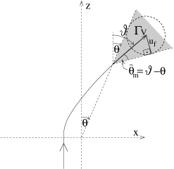
Figure 2: The Mach cone (shadowed area) with opening half-angle $\tilde{\theta}_{\rm m}=\vartheta-\theta$. The $\Gamma v_{\theta}=\Gamma v\sin\tilde{\theta}_{\rm m}$ component of the flow proper velocity equals $u_{\rm f}$ (radius of cycle).

A more robust perspective is to notice that ${\cal D}=0$ implies that the $\hat{\theta}$ component of the flow proper velocity ($\Gamma v_{\theta}/c$) is equal to the comoving proper phase velocity of a magnetosonic wave $u_{\rm f}$. Equivalently, the lines $\theta=$ constant intersect the streamlines at every point at the Mach angle $\tilde{\theta}_{\rm m}$, i.e., $\tilde{\theta}_{\rm m}=\vartheta-\theta$, see Fig. 2. This can be seen by noting that $\Gamma v_{\theta}/c=(\Gamma v/c)\sin(\vartheta-\theta)$ and $u_{\rm f}=(\Gamma v/c)\sin\tilde{\theta}_{\rm m}$ (see equation 43 of Appendix A).
The two sides of the Mach cone are the two characteristics, with equations

$$\frac{dx}{dz}=\tan\left(\vartheta\pm\tilde{\theta}_{\rm m}\right)\,,\ \mbox{ or, }\ \ \frac{rd\theta}{dr}=\tan\left(\vartheta-\theta\pm\tilde{\theta}_{\rm m}\right)\,.$$ (33)

For $\tilde{\theta}_{\rm m}=\vartheta-\theta$ we again conclude that the minus characteristics are the cones $\theta=$ constant.

Suppose we are interested to model an outflow approaching a corner, see Fig. 1. The flow is initially uniform, in pressure equilibrium with its environment (the $z<0$ regime in Fig. 1), and superfast-magnetosonic (the bulk velocity is higher than the fast-magnetosonic wave speed). In such a flow the information is propagating in a Mach cone around the flow speed, formed by the plus and minus characteristics. The effect of the corner is propagated only downstream of the minus characteristic that leaves the corner, and corresponds to the head of the rarefaction shown in Fig. 1. Each fluid parcel keeps moving with constant speed till it crosses this line. From this point on the streamlines start to bent, the flow expands and its density, thermal/magnetic energy flux decline. As a result of the energy conservation the flow is accelerated. This mechanism of converting thermal/magnetic energy into kinetic energy of bulk motion is dubbed rarefaction acceleration by Komissarov et al. (2010). The bending of streamlines and the acceleration of the flow continues till the angle $\theta=\theta_{t}$, the tail of the rarefaction, where the flow becomes ballistic and pressureless (in equilibrium with the vacuum).

Mathematically, in the initial uniform superfast-magnetosonic part of the outflow $(-\pi<\theta<-\pi/2)$, ${\cal D}$ is positive. The same is true in the first portion of the $\theta>-\pi/2$ regime. However, as the flow moves in that part (see Fig. 1) the $\hat{\theta}$ component of the flow velocity decreases leading to a decreasing ${\cal D}$ (see equation 32). Eventually ${\cal D}$ becomes zero at an angle $\theta=\theta_{h}$ corresponding to the head of the rarefaction, and remains zero in the whole rarefaction phase (for $\theta_{h}\leq\theta\leq\theta_{t}$). The system of equations (16), (20), (23), (27) gives $f$, $\vartheta$, $h$, $\sigma$ at each $\theta\in\left[\theta_{h}\,,\theta_{t}\right]$. These expressions, together with their simplified versions in the limits of cold and unmagnetized flows, are given in Appendix B.

3.2 The $\lambda>1$ case

The $\lambda=1$ is the most important case (and the only one with finite density at the corner), but we kept the analysis more general including $\lambda>1$ cases (for $\lambda<1$ the density becomes infinity at the origin). In these cases the flow is nonuniform initially, with the density increasing with the distance from the corner. As a result, denser parts tend to move towards the less dense regions, and the resulting flow expansion provides an additional acceleration mechanism on top of the rarefaction acceleration which is still present.

4 Results – Application to GRB jets

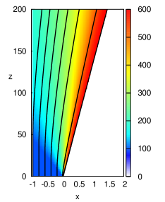
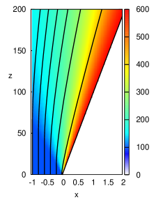
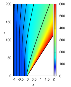
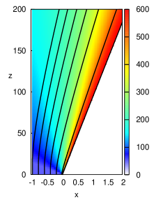
Figure 3: Solutions for the rarefaction wave $\lambda=1$. The last row shows the distribution of the Lorentz factor (color) and the streamlines (solid lines). All cases correspond to energy-to-mass flux ratio $\mu=600$. The scale of the distances is arbitrary. A convenient choice for the unit of distances is the jet radius $\sim R_{\star}/\Gamma_{j}$, in which case the $x=-1$ line mimics the rotation axis of the jet.

The numerical procedure is to give the model parameters $\lambda$, $\gamma$, the initial quantities $\Gamma_{j}$, $\sigma_{j}$, $h_{j}$, and $\vartheta_{j}$ at some initial angle $\theta_{j}$, and find $\mu$ and $f_{j}$ using equations (14), (23). Then solve the system of the two algebraic equations (16), (23) together with the two differential equations (20), (27) for the functions $f(\theta)$, $\vartheta(\theta)$, $h(\theta)$, $\sigma(\theta)$.

Since we are interested to apply the model to GRB outflows we set the energy-to-mass flux ratio ($\mu$), which equals the maximum possible bulk Lorentz factor if all the energy is transferred to kinetic, a few hundreds. In particular, we choose a value $\mu=600$ in the numerical results.

A jet associated with a long/soft GRB is thought to be formed inside the progenitor star, and its first acceleration phase takes place before it crosses the stellar surface. We take as a reference value for the resulting bulk Lorentz factor, which is the initial value for the rarefaction acceleration phase that we examine, $\Gamma_{j}=100$. For a cold flow ($h_{j}=0$) the magnetization is $\sigma_{j}=5$ such that equation (14) is satisfied. Since the details of the acceleration phase inside the star are not known in general, we also examine a model with $\Gamma_{j}=50$ (and $\sigma_{j}=11$).

If the jet is magnetically driven, it is superfast-magnetosonic when it crosses the stellar surface. It is well known from the MHD theory that in this regime the magnetic field is predominantly azimuthal, justifying our choice for ignoring the $B_{x}$ and $B_{z}$ components in the model. By adopting a planar geometry we ignore the tension of the azimuthal magnetic field. This is reasonable, since the fast variations induced by the rarefaction wave give a much larger magnetic pressure gradient in the radial ($x$) direction.

We also include a purely hydrodynamic model with $\sigma_{j}=0$ and $h_{j}=6$ (from equation [14]), and an intermediate case with $\sigma_{j}=2$ and $h_{j}=2$.

In all cases we started the integration from $\theta_{j}=-\pi/2$, with a flow parallel to the $z$ axis, $\vartheta_{j}=0$.

The results of the numerical integration for the rarefaction case $\lambda=1$ are shown in Fig. 3 for various sets of the initial quantities $\Gamma_{j}$, $\sigma_{j}$ and $h_{j}\equiv w_{j}/\rho_{j}c^{2}$. The first column corresponds to the cold/magnetized case, the third to the hydrodynamic/unmagnetized, and the middle to the intermediate case. In each column the top panels show the variation of the three parts of the energy-to-mass flux ratio (whose sum is the constant $\mu$): the bulk kinetic (including the rest mass energy) which is the Lorentz factor, the Poynting which is written through the magnetization as $h\Gamma\sigma$, and the enthalpy $(h-1)\Gamma$. During the rarefaction phase the bulk acceleration to its full completion ($\Gamma=\mu$) is clearly seen.

The bottom panels show the geometry of the flow (the solid lines are streamlines), together with the Lorentz factor (color). In agreement with the discussion in Section 3.1, three distinct regimes can be observed. The first is the unperturbed flow region ($-\pi/2\leq\theta\leq\theta_{h}$) where $\Gamma=\Gamma_{j}$. The second is the rarefied region ($\theta_{h}\leq\theta\leq\theta_{t}$) where $\Gamma$ increases. The perturbed region does not fill the whole space; there is a maximum angle $\theta_{t}$ – the so-called Prandtl-Meyer angle, or the tail of the rarefaction – leaving the rest of the area ($\theta>\theta_{t}$) void.

The pressure equilibrium at the contact discontinuity between the flow and the void space ($\theta=\theta_{t}$) implies that the thermal and magnetic pressures vanish. Consequently the flow is ballistic along the streamline that pass through the corner, and the whole energy flux has been already transferred to kinetic energy flux ($\Gamma=\mu$). All other streamlines are starting to bent when they cross the head of the rarefaction and asymptotically they become parallel to the tail. During this phase the flow is accelerating, reaching $\Gamma=\mu$ asymptotically. The spatial scale in which this acceleration takes place strongly depends on the magnetization of the flow, something that has important consequences for the applications of the model. The bottom panels of Fig. 3 show that the cold/magnetized case (first column) is accelerated much faster compared to the hydrodynamic case (third column), with the intermediate case (second column) lying between these two limiting cases as expected. For example, when the streamline starting from $x_{i}=-0.02$ reaches $z=200$ it has already $\Gamma\approx\mu$ in the former case, while in the later $\Gamma<\mu/2$.

Figure 4: The Lorentz factor as function of the starting position of each fluid parcel on the $x$ axis ($x_{i}$), for various $z$, and for two models: a cold/magnetized case (left) and a hydrodynamic case (right). The scale of the distances is arbitrary.

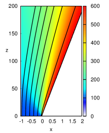
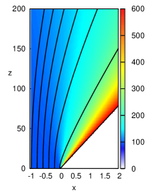
Figure 5: Similarly to Fig. 3, but for two solutions with $\lambda=2$.

The numerical results are in a perfect agreement with the analytical relations given in Appendix B and summarized below. For the cold/magnetized case which is the most important and most efficient, the head of the rarefaction wave is located at $\theta_{h}=-\sigma_{j}^{1/2}/\Gamma_{j}$ (corresponding to the half-opening angle of the Mach cone for the fast-magnetosonic waves, see Appendix A). The tail is located at $\theta_{t}=2\sigma_{j}^{1/2}/\Gamma_{j}(1+\sigma_{j})$. Note that this angle is always smaller than $1/\Gamma_{j}$. If the flow inside the progenitor star is magnetically accelerated then its half-opening angle is expected to be $1/\Gamma_{j}$ (Komissarov et al., 2009). Since $\theta_{t}<1/\Gamma_{j}$, the rarefaction increases the Lorentz factor without affecting much the opening angle, meaning that the product of the Lorentz factor with the half-opening angle increases up to the value $\sim\mu/\Gamma_{j}$ when the Lorentz factor attains its maximum value $\mu$.
As shown in the Appendix B during the acceleration the magnetization decreases as $\sigma=f^{-2/3}$, where $f$ is proportional to the distance from the corner. A streamline starting at $x_{i}$ on the $x$ axis crosses the head of the rarefaction at $r_{i}=x_{i}/\theta_{h}$. Thus, $\sigma/\sigma_{j}=(r\theta_{h}/x_{i})^{-2/3}$ and we get an analytical approximate expression for the Lorentz factor

$$\Gamma=\frac{\mu}{1+\left(\sigma_{j}\Gamma_{j}x_{i}/r\right)^{2/3}}\,.$$ (34)

The distance $|x_{i}|$ spans a range from zero – corresponding to the corner – up to a maximum value corresponding to the distance between the corner and the rotation axis of the jet, i.e., the jet radius, which can be approximated as $R_{\star}/\Gamma_{j}$. At distance $r=\sigma_{j}\Gamma_{j}|x_{i}|$ from the corner along each streamline (i.e., for each $x_{i}$), the Lorentz factor reaches half of its maximum value. As expected, fluid parcels on streamlines that are closer to the corner accelerate faster.
In terms of the streamline shape, equation (55) gives the analytical approximate relation between the Lorentz factor and the angle $\vartheta$ between the flow speed and its initial orientation,

$$\Gamma=\frac{\mu}{1+\sigma_{j}\left(1-\vartheta/\theta_{t}\right)^{2}}\,.$$ (35)

In the hydrodynamic case the angle $|\theta_{h}|$ is smaller because the sound speed is smaller compared to the fast-magnetosonic speed. As a result the acceleration phase starts later and needs larger distances to reach completion. During the acceleration a combination of equations (56) and (58) gives the Lorentz factor as a function of $r$. For $\gamma=4/3$ and $\Gamma\geq\mu/2$ we get the approximate result $r\propto\varrho^{-7/6}$ and thus $\Gamma=\frac{\mu}{1+{\cal C}(x_{i}/r)^{2/7}}$, with constant ${\cal C}$. From this expression it is evident that the acceleration is much slower compared to the magnetized case.

Fig. 4 shows the result of the acceleration across the jet, for two models. Clearly the cold/magnetized case (left panel) is much faster accelerated compared to the hydrodynamic case (right panel). Choosing the radius of the jet $(\sim R_{\star}/\Gamma_{j})$ as the unit of distances we can find the Lorentz factors in dimensional $z$, and also estimate the efficiency of the acceleration in the whole jet (which equals to the mean value of $\Gamma$ over $\mu=600$). For example, at $z=100R_{\star}/\Gamma_{j}=7\times 10^{11}$ $(R_{\star}/10R_{\odot})(100/\Gamma_{j})$ cm the mean $\Gamma$ is $\sim 200$ in the cold/magnetized case, and the total efficiency $\sim 1/3$.

The last column of Fig. 3 corresponds to a cold/magnetized case with smaller $\Gamma_{j}$ and higher $\sigma_{j}$ (such that $\mu=\Gamma_{j}(1+\sigma_{j})$ remains the same as in the other cases). It is interesting to note that, since $\Gamma_{j}\sigma_{j}$ is approximately the same as before, the dependence of $\Gamma$ on $r$ remains the same, see equation (34).

Fig. 5 shows two solutions with $\lambda>1$, one cold/magnetized (first column) and one hydrodynamic (second column). The initial flow in not uniform now, with the density increasing as we move away from the corner along constant $\theta$. This allows for redistribution of the streamlines and acceleration even before the head of the rarefaction is crossed. This is indeed seen in the figures, in both the initial increase of the Lorentz factor as well as in the bending of the flow. However, besides the initial phase the flows are very similar to the corresponding rarefaction cases $\lambda=1$.

5 Summary and Discussion

In the present paper we develop a model for the steady-state, relativistic, magnetohydrodynamic rarefaction wave. We use the method of self-similarity to reduce the system of partial differential equations to ordinary ones, which we then solve numerically. The model is a generalization of existing works for unmagnetized and nonrelativistic gas and can be applied in cases where plasma flows around a corner (equivalently it loses its external support at some position).

We apply the model to long/soft GRB jets, which are formed inside the progenitor star and lose their external support when they cross the stellar surface. In particular, we used the model and successfully interpret the results of recent numerical simulations that show a spurt of acceleration in these jets, and more generally, whenever a contact discontinuity with a relativistic flow along its plane is present.

Between models with the same energy-to-mass flux ratio we find that the rarefaction acceleration is much faster in magnetized than in hydrodynamic flows. Analytical scalings derived in Appendix B helped to quantify this behavior. For the cold/magnetized case we find that the flow reaches $\Gamma=\mu/2$ (half of its maximum value, i.e., 50% efficiency of acceleration) at distance

$$r=\sigma_{j}\Gamma_{j}|x_{i}|=7\times 10^{11}\sigma_{j}\left(\frac{|x_{i}|}{R_{\star}/\Gamma_{j}}\right)\left(\frac{R_{\star}}{10R_{\odot}}\right)\mbox{ \rm cm.}$$ (36)

The above rough estimation corresponds to $|x_{i}|=R_{\star}/\Gamma_{j}$ being the distance of the corner from the rotation axis, and $R_{\star}=10R_{\odot}$ for the stellar radius. (For the hydrodynamic case this distance is a few orders of magnitude larger.)

Our model assumes planar geometry and symmetry, which only locally hold near the points where the surface of the jet intersects the stellar surface. Improvements include axisymmetric studies, and also to take into account the reflection of the wave on the rotation axis, which will possibly cause the Lorentz factor to saturate at a value smaller than the maximum (a crude approximation of the time needed for the information to start from a fluid parcel passing the corner, hit the axis and come back at the same parcel is $\sim 2(R_{\star}/\Gamma_{j})/|\theta_{h}|\sim 2R_{\star}/\sigma_{j}^{1/2}$). Axisymmetric studies are inherently nonuniform (one of the reasons being that the magnetization vanishes on the rotation axis where the azimuthal magnetic field should be zero). For this reason comparison of numerical simulations of axisymmetric jets with our model that assumes a uniform jet initially should be done with caution at distances far away from the corner.

Another limitation is the assumption of a zero external pressure outside the progenitor star. A finite external pressure will create a standing shock and a contact discontinuity between the jet and its environment, and also limit the terminal Lorentz factor to some value smaller than its maximum. Our model cannot capture this inherently non-self-similar geometry. Nevertheless it describes the basic physics of the mechanism and gives quantitatively correct results for most of the rarefaction acceleration phase, till the point where the shock is crossed. Since the pressure contrast inside and outside the progenitor star is expected to be high, only the small shocked outflow part cannot be described by our model.

All our findings are very similar to the ones discussed in Komissarov et al. (2010). This is surprising at first, since their study is time dependent and one dimensional in space, while ours is steady-state and two dimensional in space. The reason for this similarity is the so-called frozen pulse approximation, first introduced by Piran et al. (1993) for a relativistic hydrodynamic flow and extended by Vlahakis & Königl (2003) for the full relativistic MHD case. According to this approximation, when a time dependent flow is ultrarelativistic and superfast-magnetosonic, it can be described using steady-state equations. The full mathematical proof can be found in Appendix C. The physical reason is that each part of the flow moves practically with $c$ and cannot communicate with neighboring parts through fast-magnetosonic waves (which also move at most with $c$). Thus, a possible time dependence of the flow quantities at some point of space is carried with the flow as a frozen pulse, and the motion of each part is effectively time independent.

Appendix A Fast Magnetosonic waves

Suppose that we study a magnetosonic disturbance on the poloidal plane. Its phase speed in the comoving is $\omega_{\rm co}/k_{\rm co}=\pm c_{\rm f}$ with

$$c_{\rm f}=c\sqrt{\frac{\sigma(1+u_{s}^{2})+u_{s}^{2}}{(1+u_{s}^{2})(1+\sigma)}}$$ (37)

(e.g., using the expressions given in Appendix C of Vlahakis & Königl 2003 for propagation normal to the magnetic field, $\mn@boldsymbol{k}_{\rm co}\bot\mn@boldsymbol{B}_{\rm co}$). Here $\sigma=B_{\rm co}^{2}/4\pi h\rho c^{2}$ and $B_{\rm co}^{2}=B^{2}-E^{2}=B^{2}/\Gamma^{2}$. The corresponding proper speed (over $c$) is

$$u_{\rm f}=\frac{c_{\rm f}/c}{\sqrt{1-c_{\rm f}^{2}/c^{2}}}=\sqrt{\sigma(1+u_{s}^{2})+u_{s}^{2}}\,.$$ (38)

Since the propagation is isotropic, the group velocity is equal to the phase velocity, $v_{g\,{\rm co}}=c_{\rm f}$.

Transforming the dispersion relation to the central object’s frame, we get

$$\frac{\Gamma\left(\omega-\mn@boldsymbol{v}\cdot\mn@boldsymbol{k}\right)}{\sqrt{c^{2}k^{2}-\omega^{2}}}=\pm u_{\rm f}\,,$$ (39)

or equivalently

$$\frac{\omega/k-\mn@boldsymbol{v}\cdot\mn@boldsymbol{k}/k}{1-\omega\mn@boldsymbol{v}\cdot\mn@boldsymbol{k}/k^{2}c^{2}}=\pm\frac{cu_{\rm f}}{\sqrt{1+u_{\rm f}^{2}+(\Gamma\mn@boldsymbol{v}\times\mn@boldsymbol{k}/ck)^{2}}}\,.$$ (40)

The group velocity in the central object’s frame can be found from the transformation of the Lorentz factors $\Gamma_{g\,{\rm co}}=\Gamma\Gamma_{g}\left(1-\mn@boldsymbol{v}\cdot\mn@boldsymbol{v}_{g}/c^{2}\right)$, or,

$$\frac{1}{\sqrt{1-c_{\rm f}^{2}/c^{2}}}=\frac{\Gamma\left(1-vv_{g}\cos\theta_{\rm m}/c^{2}\right)}{\sqrt{1-v_{g}^{2}/c^{2}}}\,,$$ (41)

where $\theta_{\rm m}$ is the angle between $\mn@boldsymbol{v}_{g}$ and the flow direction. The above equation can be solved for $v_{g}$:

$$v_{g}=\frac{\Gamma^{2}v\cos\theta_{\rm m}\pm\sqrt{u_{f}^{2}+1}\sqrt{c^{2}u_{f}^{2}-\Gamma^{2}v^{2}\sin^{2}\theta_{\rm m}}}{u_{f}^{2}+1+(\Gamma v/c)^{2}\cos^{2}\theta_{\rm m}}\,.$$ (42)

All directions $\theta_{\rm m}$ which give real values for the group velocity form a Mach cone around the flow direction, with half-opening $\tilde{\theta}_{\rm m}$ (the maximum allowed $\theta_{\rm m}$) given by

$$\sin\tilde{\theta}_{\rm m}=\frac{u_{\rm f}}{\Gamma v/c}=\frac{\sqrt{\sigma(1+u_{s}^{2})+u_{s}^{2}}}{\Gamma v/c}\,.$$ (43)

Note that the result is a direct generalization of the nonrelativistic $\sin\tilde{\theta}_{\rm m}=c_{\rm f}/v$, with the proper speeds replacing their Newtonian counterparts (Königl, 1980).

An alternative way to find $\tilde{\theta}_{\rm m}$ follows:
Assume a system of coordinates on the poloidal plane such that $\hat{z}$ is along the flow velocity and $\hat{x}$ normal to it. (Note that this is not the same with the $x-z$ system of coordinates adopted in the main body of the paper, in which the velocity makes an angle $\vartheta$ with the $z$ axis.) Consider a disturbance starting at $t=0$ from the line $x=z=0$ (for all $y$). In the comoving frame the disturbance starts at $t_{\rm co}=0$ from the line $x_{\rm co}=z_{\rm co}=0$, and after some time $t_{\rm co}>0$ affects a cylindrical regime $z_{\rm co}^{2}+x_{\rm co}^{2}=c_{\rm f}^{2}t_{\rm co}^{2}$, since its group velocity is $v_{g\,{\rm co}}=c_{\rm f}$ (given by 37). In the central object’s frame that regime is Lorentz transformed to $\Gamma^{2}(z-vt)^{2}+x^{2}=c_{\rm f}^{2}\Gamma^{2}(t-vz/c^{2})^{2}$, or equivalently to the elliptic cylinder

$$\frac{(\Gamma^{2}+u_{\rm f}^{2})^{2}}{(1+u_{\rm f}^{2})u_{\rm f}^{2}c^{2}t^{2}}\left(z-\frac{\Gamma^{2}vt}{\Gamma^{2}+u_{\rm f}^{2}}\right)^{2}+\frac{\Gamma^{2}+u_{\rm f}^{2}}{u_{\rm f}^{2}c^{2}t^{2}}x^{2}=1\,,$$ (44)

an equation of the form ${\cal F}(x,z,t)=0$. The area to which the disturbance is propagating is limited by the envelope of these elliptic cylinders. Solving the system ${\cal F}(x,z,t)=0=(\partial/\partial t){\cal F}(x,z,t)$ we find the two characteristic planes $x/z=\pm u_{\rm f}/\sqrt{\Gamma^{2}-1-u_{\rm f}^{2}}$, and thus the angle $\tilde{\theta}_{\rm m}$ between the envelope and the flow velocity is given by

$$\tan\tilde{\theta}_{\rm m}=\frac{u_{\rm f}}{\sqrt{\Gamma^{2}-1-u_{\rm f}^{2}}}\,,$$ (45)

an expression equivalent to 43.
(The substitution of $x=v_{g}t\sin\theta_{\rm m}$ and $z=v_{g}t\cos\theta_{\rm m}$ in equation 44 is an alternative way to find equation 42 for the group velocity in each direction.)

Appendix B The MHD rarefaction wave

Here we give the equations that characterize the rarefaction regime $\theta_{h}\leq\theta\leq\theta_{t}$ (for the case $\lambda=1$).

The head of the rarefaction corresponds to $\theta=\theta_{h}$. Since $\theta_{h}=-\tilde{\theta}_{\rm m}$,

$$\theta_{h}=-\arcsin\frac{u_{{\rm f}j}}{\Gamma_{j}v_{j}/c}$$ (46)

(using expression 43 of Appendix A). Here subscripts “j” refer to the uniform initial phase.

Using the normalized density $\varrho\equiv\rho/\rho_{j}$ as the independent variable, equation (16) gives

$$h=1+\left(h_{j}-1\right)\varrho^{\gamma-1}\,,\quad\sigma=\frac{\sigma_{j}h_{j}\varrho}{1+\left(h_{j}-1\right)\varrho^{\gamma-1}}\,,$$ (47)

equation (27) (which simplifies to ${\cal D}=0$) gives

$$f=\frac{1}{h\sigma u_{\rm f}}$$ (48)

with $u_{\rm f}=\sqrt{\displaystyle\frac{h_{j}\sigma_{j}\varrho+\left(\gamma-1\right)\left(h_{j}-1\right)\varrho^{\gamma-1}}{1+\left(2-\gamma\right)\left(h_{j}-1\right)\varrho^{\gamma-1}}}$,
equation (23) gives $\vartheta$ through

$$\sin^{2}(\vartheta-\theta)=\sin^{2}\tilde{\theta}_{\rm m}=\frac{u_{\rm f}^{2}}{\Gamma^{2}-1}$$ (49)

with $\Gamma=\displaystyle\frac{h_{j}\Gamma_{j}(1+\sigma_{j})}{1+\left(h_{j}-1\right)\varrho^{\gamma-1}+\sigma_{j}h_{j}\varrho}$,
and the differential equation (20) implies

$$\theta=\theta_{h}+\int_{\varrho}^{1}\frac{1}{\sqrt{\Gamma^{2}-1-u_{\rm f}^{2}}}\frac{d\left(\varrho u_{\rm f}\right)}{d\varrho}\frac{d\varrho}{\varrho}\,.$$ (50)

At the tail of the rarefaction wave $\varrho=0$ the thermal and magnetic energy fluxes vanish ($h=1$ and $\sigma=0$) while $f\rightarrow\infty$ and $\vartheta=\theta$. The position of the tail is $\theta=\theta_{t}$ with

$$\theta_{t}=\theta_{h}+\int_{0}^{1}\frac{1}{\sqrt{\Gamma^{2}-1-u_{\rm f}^{2}}}\frac{d\left(\varrho u_{\rm f}\right)}{d\varrho}\frac{d\varrho}{\varrho}\,.$$ (51)

The $x$ component of the velocity is $v_{x}=v_{r}\sin\theta+v_{\theta}\cos\theta$ with $v_{\theta}/c=u_{\rm f}/\Gamma$ and $v_{r}/c=\sqrt{\Gamma^{2}-1-u_{\rm f}^{2}}\ /\Gamma$.

For a highly superfast-magnetosonic and ultrarelativistic flow $\Gamma^{2}\gg 1+u_{\rm f}^{2}$ the relation $\theta-\varrho$ simplifies to

$$\theta=-\frac{u_{{\rm f}j}}{\Gamma_{j}}+\int_{\varrho}^{1}\frac{1}{\Gamma\varrho}\frac{d\left(\varrho u_{\rm f}\right)}{d\varrho}d\varrho=-\frac{u_{\rm f}}{\Gamma}+\frac{v_{x}}{c}\,,$$ (52)

where $v_{x}/c=$

$$\frac{\int_{\varrho}^{1}\sqrt{\left[h\sigma+\left(\gamma-1\right)\left(h-1\right)\right]\left[1+(2-\gamma)(h-1)\right]}\frac{d\varrho}{\varrho}}{h_{j}\Gamma_{j}(1+\sigma_{j})}\,.$$ (53)

B.1 The ultrarelativistic cold MHD limit

In that limit $(h=1)$ the previous expressions can be greatly simplified. We find $\sigma=\sigma_{j}\varrho$, $\Gamma=\Gamma_{j}(1+\sigma_{j})/(1+\sigma_{j}\varrho)$, $u_{\rm f}=\sigma^{1/2}$, $f=\sigma^{-3/2}$, and if the flow is highly superfast-magnetosonic and ultrarelativistic $\Gamma^{2}\gg 1+\sigma$,

$$\theta=\frac{2\sigma_{j}^{1/2}-3\sigma^{1/2}-\sigma^{3/2}}{\Gamma_{j}(1+\sigma_{j})}\,.$$ (54)

For the head $(\sigma=\sigma_{j})$ we get $\theta=\theta_{h}=-{\sigma_{j}^{1/2}}/{\Gamma_{j}}$, and for the tail $(\sigma=0)$ we find $\theta=\theta_{t}=2|\theta_{h}|/(1+\sigma_{j})$.
The direction of the flow is given by

$$\vartheta=2\frac{\sigma_{j}^{1/2}-\sigma^{1/2}}{\Gamma_{j}(1+\sigma_{j})}\,.$$ (55)

The streamlines in the rarefaction regime $(\theta>\theta_{h})$ are (in polar coordinates) $r=r_{\Psi}f=r_{\Psi}\sigma^{-3/2}$, or,

$$\theta=\frac{2\sigma_{j}^{1/2}-3(r/r_{\Psi})^{-1/3}-(r/r_{\Psi})^{-1}}{\Gamma_{j}(1+\sigma_{j})}\,.$$

Different values of $r_{\Psi}$ give different streamlines. For a streamline that crosses the angle $\theta_{h}$ at $x=x_{i}$ we get $r_{i}=x_{i}/\theta_{h}$ and $r_{\Psi}=r_{i}/f_{j}=\sigma_{j}\Gamma_{j}|x_{i}|$.

B.2 The ultrarelativistic HD limit

For the unmagnetized case ($\sigma=0$) similar approximations yield

$$h=1+\left(h_{j}-1\right)\varrho^{\gamma-1}\,,\quad\Gamma=\frac{h_{j}\Gamma_{j}}{1+\left(h_{j}-1\right)\varrho^{\gamma-1}}\,,$$ (56)

and if the flow is highly superfast-magnetosonic and ultrarelativistic $\Gamma^{2}\gg 1+u_{s}^{2}$

$$\theta=\frac{-hu_{s}+\int_{\varrho}^{1}\sqrt{\left(\gamma-1\right)\left(h-1\right)\left[1+(2-\gamma)(h-1)\right]}\frac{d\varrho}{\varrho}}{h_{j}\Gamma_{j}}\quad$$ (57)

$$=\frac{{\cal I}\left[\left(2-\gamma\right)\left(h_{j}-1\right)\right]-{\cal I}\left[\left(2-\gamma\right)\left(h_{j}-1\right)\varrho^{\gamma-1}\right]}{h_{j}\Gamma_{j}\left(\gamma-1\right)^{1/2}\left(2-\gamma\right)^{1/2}}-\frac{hu_{s}}{h_{j}\Gamma_{j}}\,,$$

where ${\cal I}\left[\zeta\right]\equiv\zeta^{1/2}\left(1+\zeta\right)^{1/2}+\ln\left[\zeta^{1/2}+\left(1+\zeta\right)^{1/2}\right]$.
For the head $(\varrho=1)$ we get $\theta=\theta_{h}=-{u_{sj}}/{\Gamma_{j}}$ and for the tail $(\varrho=0)$ we find $\theta=\theta_{t}=\displaystyle\frac{{\cal I}\left[\left(2-\gamma\right)\left(h_{j}-1\right)\right]}{h_{j}\Gamma_{j}\left(\gamma-1\right)^{1/2}\left(2-\gamma\right)^{1/2}}\,.$
For the distance form the corner we get

$$\frac{r}{x_{i}/\theta_{h}}=\frac{f}{f_{j}}=\varrho^{-(\gamma+1)/2}\sqrt{\frac{1+\left(2-\gamma\right)\left(h_{j}-1\right)\varrho^{\gamma-1}}{\left(\gamma-1\right)\left(h_{j}-1\right)}}\,.$$ (58)

Note that for $\gamma\rightarrow 2$, $h\rightarrow 1+\sigma$, and $h_{j}\rightarrow 1+\sigma_{j}$ we recover the relations of Section B.1 for the cold magnetized limit. This is because, for a transverse magnetic field, the magnetic pressure $B_{\rm co}^{2}/8\pi=(B^{2}/\Gamma^{2})/8\pi$ is proportional to the square of the rest mass density (see equation [9]), and thus it is analogous to a polytropic relation with index $\gamma=2$.

Appendix C Comparison with the time-dependent rarefaction wave

For $v_{y}=0$, $\mn@boldsymbol{B}_{p}=0$, and $\partial/\partial y=0$, the electric field is

$${\mn@boldsymbol{E}}=-\frac{v_{x}}{c}B\hat{z}+\frac{v_{z}}{c}B\hat{x}\,,$$ (59)

and equations (2–5) become, after some manipulation,

$$\frac{1}{c}\frac{\partial\left(\Gamma\rho\right)}{\partial t}+\frac{\partial}{\partial z}\left(\Gamma\rho\frac{v_{z}}{c}\right)+\frac{\partial}{\partial x}\left(\Gamma\rho\frac{v_{x}}{c}\right)=0\,,$$ (60)

$$\left(\frac{1}{c}\frac{\partial}{\partial t}+\frac{v_{z}}{c}\frac{\partial}{\partial z}+\frac{v_{x}}{c}\frac{\partial}{\partial x}\right)\left(\frac{B}{\Gamma\rho}\right)=0\,,$$ (61)

$$\left(\frac{1}{c}\frac{\partial}{\partial t}+\frac{v_{z}}{c}\frac{\partial}{\partial z}+\frac{v_{x}}{c}\frac{\partial}{\partial x}\right)\left(\frac{p}{\rho^{\gamma}}\right)=0\,,$$ (62)

$$\left(\frac{1}{c}\frac{\partial}{\partial t}+\frac{v_{z}}{c}\frac{\partial}{\partial z}+\frac{v_{x}}{c}\frac{\partial}{\partial x}\right)\left(h\Gamma+\frac{B^{2}}{4\pi\Gamma\rho c^{2}}\right)$$

$$=\frac{1}{\Gamma\rho c^{3}}\frac{\partial}{\partial t}\left(p+\frac{B^{2}}{8\pi\Gamma^{2}}\right)$$ (63)

$$\left(\Gamma h+\frac{B^{2}}{4\pi\Gamma\rho c^{2}}\right)\Gamma\rho v_{z}^{2}\left(\frac{1}{c}\frac{\partial}{\partial t}+\frac{v_{z}}{c}\frac{\partial}{\partial z}+\frac{v_{x}}{c}\frac{\partial}{\partial x}\right)\left(\frac{v_{x}}{v_{z}}\right)$$

$$=\left(\frac{v_{x}}{c}\frac{\partial}{\partial z}-\frac{v_{z}}{c}\frac{\partial}{\partial x}\right)\left(p+\frac{B^{2}}{8\pi\Gamma^{2}}\right)\,.$$ (64)

(The last two equations correspond to the components of the momentum equation along and normal to the flow.)
For ultrarelativistic flows with $|v_{x}|\ll|v_{z}|$ we can simplify the above system, by (i) using $v_{z}/c\approx 1$, (ii) dropping the right-hand side of equation C (since the left-hand side includes much larger terms – note that $dh=dP/\rho c^{2}$), and (iii) noting that $|v_{x}\partial/\partial z|\ll|v_{z}\partial/\partial x|$, which simplifies equation C. Careful examination of equation C reveals that the assumption $v_{z}\approx c$ holds only in the superfast-magnetosonic regime.

The resulting system gives three integrals of motion

$$-\frac{B}{\Gamma\rho c}=\Phi_{\Psi}\,,\quad\frac{p}{\rho^{\gamma}}=Q\,,\quad h\Gamma+\frac{B^{2}}{4\pi\Gamma\rho c^{2}}=\mu\,,$$ (65)

(which in principle are different for different parts of the flow), and the equations

$$\left(\frac{1}{c}\frac{\partial}{\partial t}+\frac{\partial}{\partial z}\right)\left(\Gamma\rho\frac{v_{z}}{c}\right)+\frac{\partial}{\partial x}\left(\Gamma\rho\frac{v_{x}}{c}\right)=0\,,$$ (66)

$$\mu\Gamma\rho c^{2}\left(\frac{1}{c}\frac{\partial}{\partial t}+\frac{\partial}{\partial z}+\frac{v_{x}}{c}\frac{\partial}{\partial x}\right)\frac{v_{x}}{v_{z}}=-\frac{\partial}{\partial x}\left(p+\frac{B^{2}}{8\pi\Gamma^{2}}\right).$$ (67)

By inspection of the previous equations we see that the derivatives $\partial/\partial t$ and $\partial/\partial z$ always come as a combination $\partial/c\partial t+\partial/\partial z$, and thus the variables $z$ and $ct$ can be interchanged. The steady state problem where $\partial/\partial t=0$ and the flow depends on $z$ and $x$ is mathematically equivalent to the time-dependent one-dimensional problem where $\partial/\partial z=0$ and the flow depends on $ct$ and $x$.

The above is a manifestation of the “frozen pulse” behavior of an ultrarelativistic flow, first introduced by Piran et al. (1993) for hydrodynamic flows and extended by Vlahakis & Königl (2003) in the MHD case. Due to the ultrarelativistic and superfast-magnetosonic velocity of the flow, any possible disturbance is traveling with it and cannot affect the neighboring parts. As a result the evolution of each fluid parcel is essentially steady-state. In fact, changing variables from $(x,z,t)$ to $(x,z,s)$ where $s\equiv ct-z$, we transform equations 66, 67 to

$$\frac{\partial}{\partial z}\left(\Gamma\rho\frac{v_{z}}{c}\right)+\frac{\partial}{\partial x}\left(\Gamma\rho\frac{v_{x}}{c}\right)=0\,,$$ (68)

$$\mu\Gamma\rho c^{2}\left(\frac{\partial}{\partial z}+\frac{v_{x}}{c}\frac{\partial}{\partial x}\right)\frac{v_{x}}{v_{z}}=-\frac{\partial}{\partial x}\left(p+\frac{B^{2}}{8\pi\Gamma^{2}}\right)\,,$$ (69)

which are the same with the steady-state equations in the same (ultrarelativistic) limit. Note however that the partial derivatives $\partial/\partial z$, $\partial/\partial x$ are now taken keeping $s$ (and not $t$) constant.

Since the motion is relativistic in the $z$ direction the variable $s$ is practically constant for each fluid parcel and corresponds to the time in which it passed a certain position $z_{i}$. Without loss of generality we can set $z_{i}=0$; in that case $t_{i}=s/c$. The absence of $s$ and $\partial/\partial s$ in equations 68,69 means that they do not constrain the $s$ dependence on any flow quantity ${\cal F}(x,z,s)={\cal F}(x,z,ct-z)$. This dependence is determined by the initial/boundary conditions only, i.e., by the values of the flow quantities for each fluid parcel at time $t_{i}$ when it passes $z=0$. In other words, we can find the evolution of a time-dependent flow by applying steady-state solutions to each part of the flow passing from $z=0$ at time $t_{i}=s/c$, by changing only the boundary conditions (see an example in Section 4.1.1 of Vlahakis & Königl, 2003).

In the particular case of the relativistic rarefaction wave, the frozen pulse approximation obviously holds. As a result, the steady-state solutions considered in this work can be used for the description of a time-dependent flow, and this can be achieved by simply writing the similarity variable as $z/x=(ct-s)/x=c(t-t_{i})/x$. Thus, we only need to make the substitution $z\rightarrow c(t-t_{i})$ (with constant $t_{i}$ for each part of the flow) in order to recover the equations of the time-dependent rarefaction wave with ultrarelativistic velocity in the $z$ direction, considered in Komissarov et al. (2010). The worldlines of all fluid parcels passing at time $t_{i}=0$ from the plane $z=0$ (at various $x<0$) are equivalent to the streamlines of the steady-state model. This is indeed the case in the numerical results. Choosing initial conditions as the ones in Fig. 4 of Komissarov et al. (2010) we get practically identical results, by just substituting $z\leftrightarrow ct$.

References

- Aloy & Rezzolla (2006) Aloy M. A., Rezzolla L., 2006, ApJ, 640, L115
- Cenko et al. (2010) Cenko S. B., Frail D. A., Harrison F. A., Kulkarni S. R., Nakar E., Chandra P. C., Butler N. R., et al. 2010, ApJ, 711, 641
- Chiu (1973) Chiu H. H., 1973, Physics of Fluids, 16, 825
- Granik (1982) Granik A., 1982, Physics of Fluids, 25, 1165
- Granot et al. (2011) Granot J., Komissarov S. S., Spitkovsky A., 2011, MNRAS, 411, 1323
- Kolosnitsyn & Stanyukovich (1984) Kolosnitsyn N., Stanyukovich K., 1984, Journal of Applied Mathematics and Mechanics, 48, 96
- Komissarov et al. (2010) Komissarov S. S., Vlahakis N., Königl A., 2010, MNRAS, 407, 17
- Komissarov et al. (2009) Komissarov S. S., Vlahakis N., Königl A., Barkov M. V., 2009, MNRAS, 394, 1182
- Königl (1980) Königl A., 1980, Phys. Fluids, 23, 1083
- Landau & Lifschitz (1987) Landau L. D., Lifschitz E. M., 1987, Fluid Mechanics. Pergamon Press, Oxford, §109
- Liang et al. (2008) Liang E.-W., Racusin J. L., Zhang B., Zhang B.-B., Burrows D. N., 2008, ApJ, 675, 528
- Lithwick & Sari (2001) Lithwick Y., Sari R., 2001, ApJ, 555, 540
- Lyutikov (2011) Lyutikov M., 2011, MNRAS, 411, 422
- Matsumoto et al. (2012) Matsumoto J., Masada Y., Shibata K., 2012, ApJ, 751, 140
- Mizuno et al. (2008) Mizuno Y., Hardee P., Hartmann D. H., Nishikawa K.-I., Zhang B., 2008, ApJ, 672, 72
- Pe’er et al. (2012) Pe’er A., Zhang B.-B., Ryde F., McGlynn S., Zhang B., Preece R. D., Kouveliotou C., 2012, MNRAS, 420, 468
- Piran et al. (1993) Piran T., Shemi A., Narayan R., 1993, MNRAS, 263, 861
- Racusin et al. (2009) Racusin J. L., Liang E. W., Burrows D. N., Falcone A., Sakamoto T., Zhang B. B., Zhang B., Evans P., Osborne J., 2009, ApJ, 698, 43
- Tchekhovskoy et al. (2010) Tchekhovskoy A., Narayan R., McKinney J. C., 2010, NewA, 15, 749
- Vlahakis & Königl (2003) Vlahakis N., Königl A., 2003, ApJ, 596, 1080
- Zenitani et al. (2010) Zenitani S., Hesse M., Klimas A., 2010, ApJ, 712, 951
- Zhang (2011) Zhang B., 2011, Comptes Rendus Physique, 12, 206
- Zhang & Pe’er (2009) Zhang B., Pe’er A., 2009, ApJ, 700, L65
- Zhao et al. (2011) Zhao X.-H., Li Z., Bai J.-M., 2011, ApJ, 726, 89