Electrons as probes of dynamics in molecules and clusters : a contribution from Time Dependent Density Functional Theory

Abstract

There are various ways to analyze the dynamical response of clusters and molecules to electromagnetic perturbations. Particularly rich information can be obtained from measuring the properties of electrons emitted in the course of the excitation dynamics. Such an analysis of electron signals covers observables such as total ionization, Photo-Electron Spectra (PES), Photoelectron Angular Distributions (PAD), and ideally combined PES/PAD. It has a long history in molecular physics and was increasingly used in cluster physics as well. Recent progress in the design of new light sources (high intensity, high frequency, ultra short pulses) opens new possibilities for measurements and thus has renewed the interest on these observables, especially for the analysis of various dynamical scenarios, well beyond a simple access to electronic density of states. This, in turn, has motivated many theoretical investigations of the dynamics of electronic emission for molecules and clusters up to such a complex and interesting system as C₆₀. A theoretical tool of choice is here Time-Dependent Density Functional Theory (TDDFT) propagated in real time and on a spatial grid, and augmented by a Self-Interaction Correction (SIC). This provides a pertinent, robust, and efficient description of electronic emission including the detailed pattern of PES and PAD. A direct comparison between experiments and well founded elaborate microscopic theories is thus readily possible, at variance with more demanding observables such as for example fragmentation or dissociation cross sections.

The purpose of this paper is to describe the theoretical tools developed on the basis of real-time and real-space TDDFT and to address in a realistic manner the analysis of electronic emission following irradiation of clusters and molecules by various laser pulses. After a general introduction, we shall present in a second part the available experimental results motivating such studies, starting from the simplest total ionization signals to the more elaborate PES and PAD, possibly combining them and/or resolving them in time. This experimental discussion will be complemented in a third part by a presentation of available theoretical tools focusing on TDDFT and detailing the methods used to address ionization observables. We shall also discuss the shortcomings of standard versions of TDDFT, especially what concerns the SIC problem, and show how to improve formally and practically the theory on that aspect. A long fourth part will be devoted to representative results. We shall illustrate the use of total ionization in pump and probe scenarios with fs lasers for tracking ionic dynamics in clusters. More challenging from the experimental point of view is pump and probe setups using attosecond pulses. The effort there is more on the capability to define proper signals to be measured/computed at such a short time scale. TDDFT analysis provides here a valuable tool in the search for the most efficient observables. PES and PAD will allow one to address more directly electronic dynamics itself by means of fs or ns laser pulses. We shall in particular discuss the impact of the dynamical regime in PES and PAD. We shall end this fourth part by addressing the role of temperature in PES and PAD. When possible, the results will be directly compared to experiments. The fifth part of the paper will be devoted to future directions of investigations. From the rich choice of developments, we shall in particular address two aspects. We shall start to discuss the information content of energy/angular spectra of emitted electrons in case of excitation by swift and highly charged ions rather than lasers. The second issue concerns the account of dissipative effects in TDDFT to be able to consider longer laser pulses where the competition between direct electron emission and thermalization is known to play a role as, e.g., in experiments with C₆₀. Although such questions have been superficially addressed in the simple case of alkaline clusters by means of semi-classical methods, no satisfying quantum formulation, compulsory for most realistic systems, is yet available. First encouraging results will be presented on that occasion. We shall finally give a short conclusion.

1 General introduction and physical context

Irradiation of matter constitutes a key tool in physics, chemistry, and biology, for analyzing structural and dynamical properties of atoms, molecules, clusters and bulk material. Lasers offer here an especially flexible and powerful instrument which has been widely exploited, especially during the last decades with the enormous technological progress reached in the manipulation of laser light [1, 2, 3]. We dispose now of a broad choice of laser intensities, frequencies, pulse lengths, and pulse shapes. Collisions with charged projectiles [4] are also used as sources of short electromagnetic pulses. However, they often require access to dedicated facilities.

Radiation damage is the other side of irradiation studies and it is of high current interest, for example in connection with biological tissues (”human-controlled” as in a medical context or ”natural” when referring to earth or space radiations) [5]. There are also other interesting domains of application. A typical example is the case of the irradiation of materials (especially insulators) with applications to nuclear waste management. The field is rather unexplored from the microscopic dynamical point of view and any possibility of treating irradiation scenarios on large systems would be here of invaluable help [6]. In both above examples, though, the lack of understanding of microscopic mechanisms calls for dedicated studies on prototype, finite systems. Let us cite as an example the detailed studies of irradiation of molecules of biological interest coated by a finite and well known number of water molecules [7]. The study of the irradiation of finite molecular systems and clusters is thus not only of interest for basic science but also for a wide range of practical applications.

In all cases, the immediate electronic response of the irradiated system plays a key role as the doorway to all subsequent dynamical scenarios. A basic feature is here the optical response corresponding to electronic oscillations [8, 9]. It delivers a first overview of the coupling between irradiation and matter in a large variety of dynamical situations, from gentle to strong perturbations [10, 11, 12, 13]. Optical response related to photo-absorption is the leading signal in the case of gentle perturbations. It has been explored in great detail for a large variety of electronic systems, from bulk down to atoms. For the case of stronger perturbations, further response channels, especially ionization, become highly relevant [14, 12, 15]. Still, the optical response spectrum, which characterizes the structural coupling of the system to light, provides a highly valuable information on any ensuing response mechanism, especially on ionization pattern. A typical example here is the case of resonant ionization occurring when the laser frequency comes close to an eigenfrequency of the system [14].

Equally important in energetic irradiation processes is electron transport, particularly electron emission. As typical examples, one can cite the many studies on irradiation of clusters by short and intense laser pulses [15], providing invaluable information especially through energy (Photo-Electron Spectra, PES [16]) and, more recently, angle-resolved [17] distributions of emitted electrons (Photoelectron Angular Distributions, PAD). Electron emission can also change the resonant ionization conditions in the course of time evolution which, in turn, influences back again the optical response, making the whole scenario extremely rich [15]. Secondary electrons in DNA damage [18] also provide a remarkable example where a microscopic understanding of irradiation damage in biological systems will only be achieved when including such complex non-linear electronic effects. A deeper understanding of the underlying mechanisms is highly desirable, as this example is of great practical interest, especially in relation to oncology [5].

The analysis and understanding of electronic emission from a finite system is thus a key issue in a wide range of physical, chemical and biological processes. Electrons are usually the first constituents to respond to an electromagnetic pulse. Strong excitations lead to immediate ionization of the system, often with dramatic long-time effects as, e.g., dissociation or Coulomb explosion [13]. It implies electronic transport and possible indirect effects on neighboring species. A typical example of indirect effects is provided by Dissociative Electron Attachment (DEA) in biological systems [5] where electrons emitted somewhere else are attached to a target biological molecule which, in turn, leads to the break up of the latter. Emitted electrons may also provide valuable insight into reaction pathways when properly tracked. Typical examples are here PES and PAD. Moreover, Time-Resolved (TR) PES and PAD have been recorded in molecules [19] and more recently in clusters, see e.g. [20]. Electrons are thus leading players at all stages of an excitation of a system subject to an external electromagnetic perturbation (i.e. an irradiation). They are the first to respond at short time scales and distribute then the excitation more or less quickly to other degrees of freedom. They are finally useful probes along the whole dynamical process, especially when emitted from the system and properly recorded.

Analyzing the characteristics of emission properties of clusters and molecules is thus at the core of the understanding of irradiation processes. The numerous new experimental developments in analysis of electronic emission (PES, PAD) now allow an ever improving detailed access to electron dynamics in irradiated species. In turn, a theoretical description of these highly involved dynamical scenarios calls for dedicated modeling. It is the aim of this paper to provide an overview of the theoretical description of observables from electron emission on the basis of the well established theoretical framework of Time-Dependent Density Functional Theory (TDDFT) [21]. This will be done with a view on applications, as far as possible in direct relation to ongoing experiments. Before going into the details, we will in this introductory section briefly remind the reader the typical systems (and associated scales) that we aim at describing. It is also of relevance to address here basic properties of laser pulses as presently accessible experimentally.

1.1 On the typical systems considered in this paper

In order to provide a basis for the forthcoming discussions, we shortly present here a few typical systems we shall consider in the following. This will be the occasion to remind typical scales associated to these systems, especially in terms of times and energies.

Fig. 1 provides four examples of systems computed with the tools described in Secs. 3, 4.1.1 and 4.1.2. They cover several different binding types and properties.

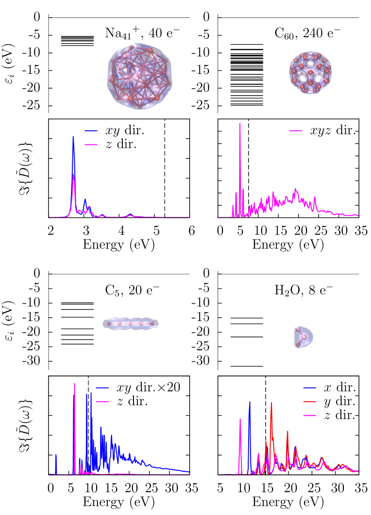
Figure 1: Four typical examples of molecules and clusters explored theoretically in this review, namely the metal cluster ${{\rm Na}_{41}}^{+}$ (upper left), the Buckminster fullerene C₆₀ (upper right), the carbon chain C₅ (lower left), and the covalent molecule H₂O (lower right). For each panel: Top row : ionic structures (all plotted at the same scale) and single particle energies of the valence electrons whose number is indicated; Bottom row : corresponding optical response. For C₅, the transverse spectrum is multiplied by 20 to ease the comparison with the longitudinal response. The vertical dashes indicate the position of the ionization potential in each case.

The figure shows single-particle (s.p.) energies, optical response and ionic structure. The four presented systems are ${{\rm Na}_{41}}^{+}$ as an example of a simple metal cluster, C₆₀ for its outstanding properties and many applications, H₂O as a prototype of a covalent molecule, and C₅ as a simple carbon chain, which displays interesting optical properties. Let us analyze each system separately to extract typical properties.

We start with the ${{\rm Na}_{41}}^{+}$ cluster (upper left block in Fig. 1) which is a medium size alkaline cluster. It contains 40 valence electrons forming an electronic shell closure. This leads to a particularly abundant/stable species. The s.p. energies span an energy range of order 2.6 eV and the Ionization Potential (IP) is of order 5.3 eV. Such values are typical of alkaline clusters. The optical response displays a pronounced collective, essentially single, peak around 2.6 eV. This is called the Mie surface plasmon and it is a typical mode for simple metal clusters. In larger clusters, the density of s.p. states grows, which leads to more Landau fragmentation and somewhat broadens the plasmon peak. The Mie plasmon frequency is related to a typical time scale of order 1.5 fs, again a characteristic time scale for simple metals. Ionic time scales (not shown in Fig. 1) are more sensitive to the actual material due to the largely differing atomic weight. In Na clusters, vibrational modes typically lie in the 10 meV range and are associated to ionic motion in the 100 fs range.

The second example is C₆₀ (upper right block) with 240 valence electrons (4 per C atom). The s.p. energies now ranges in a span of about 17.3 eV, much wider than in Na. The IP is 7.6 eV. The deeper binding and broader span of energies is typical of carbon, and more generally of organic systems with a covalent binding. Due to the high symmetry close to sphericity, the optical response exhibits the same behavior in all spatial directions. It has, however, a more complex structure than in ${{\rm Na}_{41}}^{+}$. One can identify two prominent features, a strong resonance peak just below the IP and a much broadened peak centered around 20 eV. The latter part of the optical response lies well above the IP, whence its highly fragmented structure. It is considered to represent the Mie surface plasmon in C₆₀. The energies are higher and thus the associated time scales much smaller than in Na, typically well sub-fs. Ionic vibration energies typically lie in the 40-200 meV range with associated time scales of order 20-100 fs.

The case of the small carbon chain C₅ (lower left block) is complementing C₆₀ in the sense that it has the same binding type, but a different geometry and thus different optical response. The s.p. energies span of the 20 valence electrons is of order 14 eV, and the IP of order 9.9 eV. These values are of the same order of magnitude for larger chains. According to the linear geometry of the chain, the optical response shows a dominant resonance peak along the longitudinal direction at a frequency of 6.4 eV. The transverse modes are suppressed by at least one order of magnitude (mind that transverse strengths have been multiplied by a factor of 20 to allow a better graphical comparison with the longitudinal modes) and are significantly fragmented. There are three main peaks : one at the same energy as the longitudinal plasmon peak, and two other ones at higher energies near the IP energy. The all dominant longitudinal mode lies well below the IP, a feature common to all carbon chains. Associated time scales are now typically ranging from sub-fs to fs. Ionic vibration energies lie again in the 0.15 eV range with associated time scales of order 27.6 fs.

We finally discuss the case of the prototypical water molecule H₂O (lower right block) which has 8 active valence electrons in our calculations (6 for O and 1 per each H). The s.p. energy span is now with 16 eV even larger than in C₆₀, in spite of the much smaller number of electrons. The IP is of order 15.1 eV. Such large IP’s are typical of covalent systems of small to moderate size. The optical response, as well, is typical of covalent molecules with its highly fragmented structure above the IP, and some isolated low energy peaks below the IP. Associated time scales lie well below fs. Ionic vibrations are more energetic than in other systems because of the especially light H species and the strong covalent binding between H and O. The O-H ionic vibration energy is about 0.5 eV with associated period of 8.3 fs.

All in all, the four above examples point out the diversity and richness of the various systems nowadays accessible to both experimental and theoretical investigations. The various cases also show that the range of energy and time scales to be investigated is rather large from attosecond to several fs for electrons, and from fs to ps for ions. In addition, the optical spectra exhibit different pattern. Specific for metals is the especially well marked Mie surface plasmon with simple scaling properties with size [10]. The case of covalent systems is more involved with basically no simple scaling properties, but nevertheless some generic trends. Optical spectra are generally much more fragmented below and even more so above IP. Pure carbon systems contain besides covalent binding a fraction of metallic binding which produces also plasmon structures amongst the highly fragmented spectrum.

Optical response is the key to understanding the coupling of the system to laser light, at least in the frequency-dominated regime (see Secs. 1.2 and 2.1). This will constitute a mostly used tool of investigation of dynamical scenarios in the following discussions. Before introducing the actual observables which can be attained that way, we will briefly discuss present days capabilities of lasers and the description of the electromagnetic fields they deliver. This aspect is addressed in the following Sec. 1.2.

1.2 On excitation mechanisms

Cluster dynamics requires excitation of the cluster formerly resting in its ground state. In this paper, we will exclusively addess excitation by electromagnetic fields, predominantly by laser pulses and in a few cases by short pulses from collisions with highly charged ions. The corresponding excitation mechanisms are shortly explained in this section. Thereby, we focus on laser properties and finally address ion collisions in a short paragrph.

1.2.1 Laser pulse characteristics

Laser science has experienced impressive progress during the last few decades [3]. The versatility of laser pulses has increased remarkably, thus allowing one to shape a wide range of dynamical scenarios in the course of irradiation processes. We briefly remind here key quantities of the laser pulses we are going to use in the following. Throughout this paper, we shall work in the dipole approximation which requires that the irradiated system is much smaller than the laser wavelength $\lambda=2\pi c/\omega_{\mathrm{las}}$. In practice, the dipole approximation is well justified in the optical domain ($\lambda\sim\mu$m) for systems of nm size. It may become questionable for XUV photons and very large clusters in which field variations inside the system itself should be accounted for. But we shall not consider such cases here. In the non-relativistic regime, linearly polarized laser pulses acting on atoms, molecules or clusters can then be described as a homogeneous time-dependent electric field of the form

$$\mathbf{E}(t)=\mathbf{e}_{\mathrm{pol}}\,E_{0}\,f(t)\,\sin(\omega_{\mathrm{las}}t+\varphi)\quad.$$ (1)

In this expression, $\mathbf{e}_{\mathrm{pol}}$ denotes the (linear) polarization, $E_{0}$ is the peak field strength, $\omega_{\mathrm{las}}$ is the photon frequency, and $\varphi(t)$ is some phase shift, usually assumed to be zero. Finally $f(t)$ is the pulse envelop. The peak laser intensity is $I_{0}=c\,\varepsilon_{0}\,E_{0}^{2}/2$ ($c$ being velocity of light in vacuum) usually expressed in W/cm². The net yield in a laser pulse is often characterized by the fluence $\mathcal{F}=\int\textrm{d}tI(t)\approx I_{0}T_{\mathrm{FWHM}}$, where the latter time $T_{\rm FWHM}$ stands for the Full Width at Half Maximum of the pulse. This allows one to compare the energy impact of laser pulses with different durations.

For the sake of simplicity, we keep in the present discussion a fixed value of $\omega_{\mathrm{las}}$ but the latter quantity can also be made time-dependent (”chirped”) which can induce interesting effects [3]. One may also render the phase $\varphi$ time-dependent, which could produce interesting phenomena. We shall not discuss these aspects here. The laser polarization is usually taken linear but there also exists experiments/calculations using circularly polarized light [3]. Again, we shall not discuss much such cases in the following and thus recur to a linear polarization for the present discussion.

The laser pulse envelop can be varied in a large range. Most flexible, and most widely used, are optical lasers with pulse lengths from nano-seconds down to atto-seconds [22, 23]. Free Electron Lasers (FEL) [24, 3] are yet on their way to comparable flexibility, with present pulse lengths down to 20 fs. It should also be noted that the actual shape of $f(t)$ is not exactly known experimentally. In many situations, the actual pulse of interest is built upon a (hopefully harmless) background of a long, low intensity, pulse. Moreover, the peak intensity has a spatial variation decreasing towards the edges of the pulse. This has to be kept in mind when assigning the observed signal to the laser pulse characteristics. Ignoring background, experimental short laser pulses have a pulse profile of Gaussian type. The theoretical situation is simpler as the pulse profile can be exactly specified. The Gaussian profile is theoretically not welcome since it never fully vanishes and requires unnecessarily long computation times to cover the pulse sufficiently well. Therefore, we mostly use for computations a $\sin^{2}$ pulse :

$$f(t)=\sin^{2}\left(\frac{t\pi}{T_{\mathrm{pulse}}}\right)\,\theta(t)\,\theta(T_{\mathrm{pulse}}-t)\quad.$$ (2)

where $\theta$ stands here for the Heaviside function. This pulse is limited to a finite time interval $t\in[0,T_{\mathrm{pulse}}]$, but soft enough to deliver a clean frequency spectrum. It can be simply characterized by its FWHM which is in this case $T_{\mathrm{FWHM}}=T_{\mathrm{pulse}}/2$. Note that the FWHM of the intensity $I(t)$, which is proportional to the square of the field $\mathbf{E}(t)$, is rather $T_{\rm pulse}/3$. The pulse maximum occurs at $t=T_{\mathrm{pulse}}/2$. Note that the sin² profile is written here for the laser field amplitude, which means that the time profile of the intensity time has a sin⁴ shape. Thus far, we have discussed simple one-peak pulses. More flexibility is conceivable. The next important tool are dual pulses as used in pump-and-probe experiments in which the laser irradiation is performed in two steps. We shall illustrate such cases at several places below.

In practice, the effect of the laser field will be accounted for in our calculations as an external potential $U_{\rm ext}(\mathbf{r},t)$ which delivers a time-dependent perturbation. In the long wavelength limit, the electric field is homogeneous and delivers the potential :

$$U_{\rm ext}(\mathbf{r},t)=-e\,E_{0}\,f(t)\,\sin(\omega_{\mathrm{las}}t)\,\mathbf{e}_{\mathrm{pol}}\cdot\mathbf{r}\quad,$$ (3)

where $f(t)$ is the time profile usually taken according to Eq. (2). This is, in fact, the laser field in space gauge. Equivalently, one can use the velocity gauge for which the laser field is described by the interaction operator :

$$\hat{U}_{\rm ext}^{(v)}=-\frac{e}{c}\,E_{0}\,F(t)\,\mathbf{e}_{\mathrm{pol}}\cdot\hat{\mathbf{p}}\quad.$$ (4)

The rules of gauge transformation relate time profiles and wave functions by :

$$F(t) = \displaystyle\int^{t}_{-\infty}\mathrm{d}t^{\prime}\,f(t^{\prime})\,\sin(\omega_{\mathrm{las}}t^{\prime})\quad,$$ (5)

$$\varphi_{i}^{(v)}(\mathbf{r},t) = \varphi_{i}^{\mbox{}}(\mathbf{r},t)\exp{\left[\mathrm{i}\,E_{0}\,F(t)\,\mathbf{e}_{\mathrm{pol}}\cdot\mathbf{r}\right]}\quad.$$ (6)

Both gauges are fully equivalent. Which one is to be preferred is a matter of the actual numerical scheme. Most observables are not even sensitive to gauge. An exception is the evaluation of photoelectron spectra where the phase of the wave function plays a role. In this case, one has to consider gauges carefully. This will be addressed in more detail in Sec. 3.3.

1.2.2 Varying laser characteristics

As pointed out above, all laser parameters can be tuned in rather large ranges. The point is illustrated in Fig. 2 which displays typical regions of interest in the intensity-frequency plane.

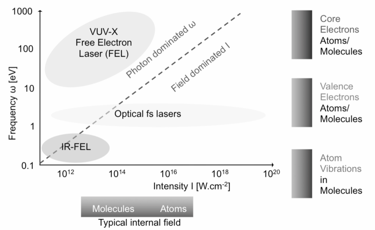
Figure 2: Schematic representation of various dynamical regimes as a function of laser intensity $I$ and photon frequency $\omega$. The dashed diagonal line represents frequency-intensity combinations with constant Keldysh parameter $\gamma=1$, see text for details. This line characterizes the transition from photon-dominated to field-dominated regime for an assumed IP of a few eV. The blocks to the right side indicate typical frequency ranges as labeled. The block below the plot indicates typical atomic field strengths related to given laser intensities.

One can notice the enormous large intensity range of optical lasers. But the range of available conditions is also dramatically extended by FEL, which exist for photons in the IR, VUV and X-ray regime. Also indicated outside the axes are corresponding regions of relevance in atoms and molecules in terms of energy/frequency and field/intensity. The lowest frequencies in the deep IR are associated with molecular vibrations, while the range around visible light belongs to the dynamics of valence electrons and core electrons move at much higher frequencies in X-ray regime. The gray box below the plot indicates typical atomic and molecular field strengths in terms of an equivalent laser intensity.

Laser characteristics have to be considered in relation to the electronic response. This is usually quantified via the ponderomotive potential $U_{p}$ and the associated Keldysh parameter $\gamma$. $U_{p}$ represents the electron kinetic energy (averaged over one photon cycle) of a freely oscillating electron (pure quiver motion, no drift velocity) in a laser field. At peak laser intensity, it reads :

$$U_{p}=\frac{e^{2}\,E_{0}^{2}}{4\,m_{\rm el}\,\omega_{\rm las}^{2}}=9.33\times 10^{-14}{\rm eV}\times\,I_{0}[{\rm W/cm^{2}}]\,(\lambda_{\mathrm{las}}[{\rm\mu m}])^{2}\quad,$$ (7)

where $\lambda_{\mathrm{las}}$ is the photon wavelength. The other aspect concerns the electronic binding in the system, which can be quantified by the ionization potential (IP) with associated energy $E_{\mathrm{IP}}$. What counts is the relation between $E_{\mathrm{IP}}$ an $U_{p}$, quantified by the Keldysh parameter [25] :

$$\gamma=\sqrt{\frac{E_{\mathrm{IP}}}{2U_{p}}}=\sqrt{\frac{2\,E_{\mathrm{IP}}\,\omega_{\mathrm{las}}^{2}}{I_{0}}}\quad.$$ (8)

The value $\gamma=1$ (see Fig. 2 in the case $E_{\mathrm{IP}}=1$ eV) separates two regimes. For $\gamma\ll 1$, direct ionization (over barrier or tunneling) prevails. This regime is dominated by laser intensity and not so much by laser frequency (field-dominated regime). For $\gamma\gg 1$, emission proceeds through multi-photon ionization in a regime of weak perturbations. There, the results sensitively depend on laser frequency (photon- or frequency-dominated regime).

1.2.3 Not on lasers: collisions with fast ions

There is an alternative excitation mechanism by collisions with charged projectiles. We shall also marginally consider a few examples of collisions with fast ions and thus comment briefly about this tool here. Experiments with charged, fast ions often require access to large scale facilities. Thus there are much less experiments with irradiation by charged projectiles than by the more easily accessible and versatile lasers. Although collisions with charged particles also provide a strong electromagnetic perturbation (often in form of a short pulse as soon as the projectile velocity is large enough), the characteristics of the perturbing field are significantly different from those delivered by a laser pulse. While lasers provide (up to details) an electromagnetic field with a well defined frequency band (basically the laser frequency), collisions with charged projectiles deliver a perturbation covering a very broad band of frequencies, the broader the shorter the pulse. This delivers useful, complementing information to that attained from lasers. It is important to note that collisions with charged projectiles also concern a wide range of potential applications of irradiation dynamics, especially in relation to radiation damage and applications thereof. The present review concentrates on laser excitations. Nevertheless, we shall discuss a few cases with high energy projectiles. For them, the delivered electromagnetic perturbation can be modeled as an instantaneous boost ($\propto\delta(t)$) at the initial time of the simulation. This is the way we shall treat this case in the following (see in particular Sec. 5.1).

2 From integrated to detailed observables

Electronic emission can be analyzed at various levels of sophistication, starting from fully integrated quantities (total ionization) down to energy-resolved (Photo-Electron Spectra, PES) and angle-resolved (Photo-Angular Distribution, PAD) quantities. Time is also a key quantity as ionization signals can be followed in time, leading to Time-Resolved (TR) results. We briefly describe in this section the various types of observables experimentally accessible, starting from the simplest one, that is the total ionization, to the most elaborate ones (TR-PES and PAD). In terms of cross sections, this means that we go from integrated ones to single-differential and even double-differential ones, all possibly time-resolved. Before discussing these various observables, we briefly introduce key mechanisms of ionization, again focusing the discussion on laser induced ionization.

2.1 Ionization mechanisms

Basic ionization mechanisms are illustrated in Fig. 3.

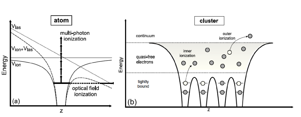
Figure 3: Schematic view of ionization mechanisms in atoms and clusters. Occupied electron states are indicated by horizontal bars. (a) : multiphoton and optical field ionization in an atom, for which are drawn the potentials of the unperturbed ion $V_{\rm ion}$ (full line), of the laser $V_{\rm las}$ (dots), and of the sum of both (dashes). (b) : inner and outer ionizations in a cluster, with the effective electron potential (without laser) shown as a solid line. Adapted from [15].

We start from the simplest case of an atom (left panel in Fig. 3) to introduce two basic ionization mechanisms. The first one corresponds to a vertical excitation of a bound electron by absorption of one or several ($\nu$) photons (Multi-Photon Ionization or MPI). This mechanisms may spread over several laser cycles and prevails in weak and moderate fields, usually quoted perturbative regime. It is associated to large values of the Keldysh parameter ($\gamma\gg 1$). MPI can promote electrons far above threshold into the continuum and then, it also stands for Above Threshold Ionization (ATI). It is a typical mechanism underlying PES and PAD measurements in the perturbative regime (see Sec. 2.3), providing mostly structural information. The second mechanism illustrated in the case of atoms is known as Optical Field Ionization (OFI) in which the laser acts as a quasi stationary field. For sufficiently large fields, bound electron can tunnel through the barrier, which means that both barrier height and width (thus tunnel characteristic time) allow ionization. This typically corresponds to moderate values of the Keldysh parameter ($\gamma\lesssim 1$). The limiting case corresponds to full barrier suppression which can be associated to a critical laser intensity in atoms and which reasonably matches ion appearance intensities in atomic gases [26].

The cases of molecules and clusters mix the above considerations with structural properties of the considered systems. For example, ionization barriers are influenced by neighbouring ions. A typical example is the case of strong field ionization of diatomic molecules [27, 28] in which an appropriate internuclear separation leads to lowering or suppression of inner and outer potential barriers, thus leading to enhanced ionization. The effect was also studied in small clusters [29, 30]. In the case of large clusters, one should also mention the separation between inner and outer ionization [31] (see right panel in Fig. 3), especially important in the case of strong fields. Inner ionization leads to the formation of a set of quasi free electrons constituting sort of a metallic phase. A final excitation may promote them to the continuum for final escape and then will appear as the total ionization of the system. In most of the cases, we shall discuss in the following we shall not consider strong enough fields to use this concept further. On the other hand, we shall deal with situations where another key ingredient, already mentioned previously, enters the picture. It concerns the optical response of the irradiated species. Indeed the optical response provides the eigenfrequencies with which a given system does couple to light. It is thus crucial to integrate it in the discussion of ionization mechanisms, especially in the case of metal clusters in which the plasmon plays a leading role.

The point is illustrated in Fig. 4 in the case of a small size sodium cluster Na₂ in which the notion of collective plasmon is hard to disentangle from that of a molecular dipole transition. Na₂ possesses two valence electrons.

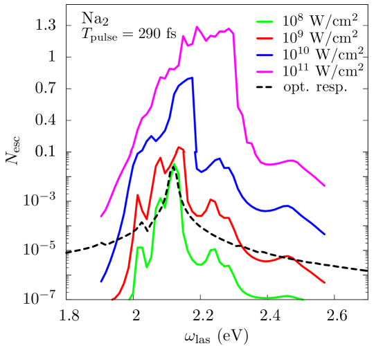
Figure 4: Total ionization $N_{\rm esc}$ of Na₂ after irradiation by laser pulses polarized along the cluster axis, with duration of 290 fs, as a function of laser frequency $\omega_{\rm las}$, for four different intensities as indicated. Dashed curve : optical response (power spectrum) of Na₂. Mind that for $N_{\rm esc}<0.1$, the vertical axis is in logarithmic scale, while a linear scale is used above 0.1.

The mechanism actually remains the same and is thus illustrative of the role of the optical response. We shall consider plasmon effects on some examples later on (see in particular Sec. 4.2.1 and Fig. 30). The dashed curve shows the optical response of the system with a well identified peak at 2.12 eV. The full curves display the total ionization as a function of laser frequency for a set various laser intensities between $10^{8}$ and 10¹¹ W/cm². One clearly observes that the ionization signal directly follows the optical response : attaching a resonance peak leads to enhanced ionization. The effect is especially visible at low intensity and vanishes with increasing intensities. We gradually leave the photon-dominated regime (low intensity) to reach the field-dominated one. In terms of the Keldysh parameter $\gamma$, it decreases. In the present test case, $\gamma$ takes values typically between 60 and 250 in the resonance region at low intensity, and reaches values between 2 and 10 in the high intensity case. The role of resonance peaks is thus crucial here and it should be noted that it does not reduce to the linear regime of excitation. The total ionization may reach rather large values (more than half of the available valence electrons) with increasing laser intensity, and still, the resonance enhancement remains very clear. This indicates that it will have to be considered whatever the dynamical regime in the following, especially in the case of metals. Although the basic enhancement mechanisms remain similar in non-metallic systems (see Sec. 4.2.1), resonances are usually less collective and more narrow so that their impact is somewhat different. Still, in many systems such as for example C₆₀, one observes a wide bunch of resonances above continuum threshold which very clearly play a key role in the dynamics.

2.2 Total ionization

Total ionization is the simplest ionization signal one can measure. Still, it already brings interesting information, although not highly detailed, on irradiation mechanisms, as we just discussed in the previous section. We here illustrate the point on two examples taken from rather original scenarios. The first case results from an irradiation with extremely large frequencies obtained from a FEL, and the second one directly addresses the dynamical evolution of the system in a time-resolved experiment.

Fig. 5 shows time-of-flight (TOF) spectra of Xe clusters irradiated by a FEL of frequency around 12 eV [32].

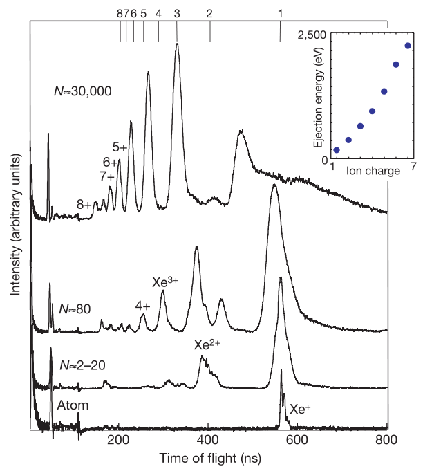
Figure 5: Time-of-flight mass spectra of ionization products of Xe atoms (bottom curve) and clusters of various sizes $N$ as indicated. Irradiation was performed by a free-electron laser of wavelength of 98 nm and an average intensity of $2\times 10^{13}$ W/cm². The line splitting of the atomic spectrum (bottom curve) is due to different isotopes. Inset : ion kinetic energies as a function of ion charge, in the case of 1500-atom clusters. From [32].

The TOF gives access to the various charge states attained after irradiation by a laser of intensity $2\times 10^{13}$ W/cm² and pulse length of 100 fs. The striking point of the figure is the differences observed between the various cluster sizes in terms of attained charge states. While the atomic gas, under the present laser conditions, only allows to access singly charged cations, increasing cluster size allows to progressively reach larger and larger charge states, clearly up to $8+$ in the largest system of about 3,000 atoms. The case very nicely illustrates the well known difference between energy absorption by single atoms and clusters, as discussed on many occasions in the past (see for example [15] and references therein). The mass peaks are rather broad. They are furthermore displaced with respect to the calculated flight times indicated by thin vertical lines (corresponding to the different charge states) in the top of the figure. This is an indication that ions have high kinetic energies. Not surprisingly, one can also note that the higher the charge state, the higher the ejection energy (see inset in Fig. 5) and the larger the above mentioned peak displacements.

Analysis of total electron emission (or alternatively of charge state of ionized clusters) also gives information on the dynamics of the charging process. One of the most striking early example of such an analysis can be found in a series of experiments led by the Rostock group on large size Pb clusters [33, 34, 35]. These experiments have shown strong enhancement of cluster ionization for optimal pulse durations. More specifically, one observed Pb ions with very large state states, much larger than those attained in an atomic gas. Moreover, the attained charge state $q$ strongly depends on the pulse duration. The shortest and most intense pulses of duration 150 fs yield ions up to charge state $q=20$. When increasing pulse duration, both the maximum charge state and the signal intensity do grow towards a maximum attained for an optimal pulse width of 800 fs. Charge states up to $q=28$ can then be identified. For longer pulses, both maximum $q$ and signal decrease again. Although other mechanisms can be envisioned, the efficient charging for a certain pulse duration was in most cases attributed to resonant heating (plasmon-enhanced ionization) [36, 37, 38, 13].

The above case of ionization enhancement was attained with a single laser pulse and only provides a rather indirect indication on the ionization mechanism. More detailed investigations were led with dual (or pump-and-probe) pulses, especially in the case of Ag clusters of about 20 000 atoms. An example of such experiments is shown in Fig. 6 where one focuses on the yield of Ag¹⁰⁺ and the maximum of the emitted electrons as a function of pulse separation.

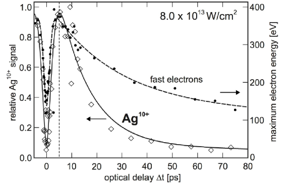
Figure 6: Ionic charge state Ag¹⁰⁺ yield (diamonds, left axis) in relation to the maximum kinetic energy of the emitted electrons (dots, right axis) following a laser excitation of Ag clusters of about 20 000 atoms with dual 100 fs laser pulses of intensity of $8\times 10^{13}$ W/cm² and wavelength of 800 nm. From [39].

One observes a strong variation of ionic signal as a function of pulse separation (delay between pump and probe) with a clear maximum around 5 ps [39]. Such a behaviour indicates that cluster activation and enhanced ionization can be clearly disentangled, which is also found in numerical simulations [40, 39, 41]. This again provides an interesting insight the dynamical evolution of the system. There are even clear indications that a sequence of two pulses might constitute an optimal pulse profile for the production of very high charge ions [42], provided a proper tuning of pulse parameters. And pushing again the argument, one can even envision a route for targeted control of the cluster dynamics [38]. Finally a word on the maximal electron energy shown in Fig. 6 is in place. The coincidence of high ionization yield and maximal electron energy again points out the leading role of collective excitations, and this in both channels. This is compatible with other observations [43, 44].

2.3 Energy- and angular-resolved ionization

The next step in the analysis of electronic emission consists in characterizing the properties of the emitted electrons in terms of kinetic energy and angular distribution. This leads to Photo-Electron Spectra (PES) for the energy analysis and Photo-Angular Distribution (PAD) for angular signals. The terms come from laser irradiation but the signals themselves can as well be recorded in any ionization scenario, for example from collisions with highly charged ions (see Sec. 5.1). PES and PAD signals turn out to provide extremely rich information, both from a structural and from a dynamical viewpoint. We briefly discuss their properties in this section and illustrate them on a few examples covering several dynamical situations.

Kinetic energies of emitted electrons can be measured in several ways. TOF devices provide here a versatile tool, but this time applied to the electrons themselves (while they are traditionally used for ions). Because of the well defined mass to charge ratio for an electron, the arrival delay directly maps the electron kinetic energy, provided a carefully guiding of the electron flow e.g., by a magnetic mirror [11]. Another very interesting technique is provided by photo-imaging spectroscopy, also known as Velocity Map Imaging (VMI). This technique is more and more routinely used and provides a remarkable tool of investigation. It is based on a static electrical field which allows one to map the distribution of electron velocities onto definite positions on a detection screen [45]. This is a polar representation of a velocity-resolved (or a momentum one) and angular-resolved photoelectron spectrum. Two experimental examples are presented in Fig. 7, one in the metal cluster ${\mathrm{Na}_{3}}^{-}$ in the monophoton regime [46], and another one in C₆₀ in the multiphoton regime [47].

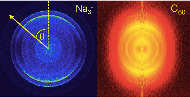
Figure 7: Left : Raw velocity map image of ${\mathrm{Na}_{3}}^{-}$ irradiated by a laser pulse of frequency of 4.02 eV and polarized vertically [46]. The length of the arrow stands for the velocity of the photoelectron, and $\theta$ its angle to the laser polarization axis. Right : Inverted momentum map image of C₆₀ irradiated by a laser pulse of FWHM of $150\pm 5$ fs, intensity of $1.25\times 10^{13}$ W/cm², frequency of 3.68 eV, and polarization along the vertical axis [47].

In these two examples, the vertical direction stands for the laser polarization axis. If one draws an arrow from the origin of the circle, its length represents the norm of the velocity (or the momentum), while the angle $\theta$ to the vertical direction is the angle of the photoelectron with respect to the laser polarization axis, and the lighter the extremum of the arrow, the higher the yield at this point. The observed circles correspond to peaks in the PES (not shown here). left panel of Fig. 7 is a raw image, while the right one is obtained after some inversion analysis. An approach such as VMI allows a simultaneous determination of PES together with PAD, which is extremely interesting. From the thus combined PES/PAD distribution (double differential, energy- and angle-resolved, cross section) it is then easy to recover PES or PAD separately by proper energy or angular integration. Still, mostly because of signal intensity, the double differential cross section can rarely be used as a whole. Therefore, energy or angular integration usually allow a simpler access to the data. It is also simpler and usually more quantitative to compare theory to experiments in simpler representations, where rather than the double differential cross section $\textrm{d}\sigma/\textrm{d}Ed\Omega$ PES/PAD, one considers singly differential PES $\textrm{d}\sigma/\textrm{d}E$ or PAD $\textrm{d}\sigma/\textrm{d}\Omega$ cross sections. We shall thus explore now in more detail integrated PES and PAD.

2.3.1 Photoelectron spectroscopy

A PES typically results from a multiphoton ionization (MPI) mechanism (see Sec. 2.1). Electrons absorb a certain number of photons to reach the continuum and be emitted. They can absorb more than the number of photons required to reach the continuum threshold, which leads to copies of the signal (although much reduced in intensity). The kinetic energies of the emitted electrons are then directly related to the single electron energies $\varepsilon_{i}$ of the initially occupied electron states $i$ inside the cluster through the simple relation :

$$\varepsilon_{\rm kin}=\varepsilon_{i}+\nu\hbar\omega_{\rm las}\quad,$$ (9)

where $\nu$ is the number of photons involved in the process.

Fig. 8 illustrates the principle of PES in terms of a scheme (left part), both in the case of mono- and multi-photons.

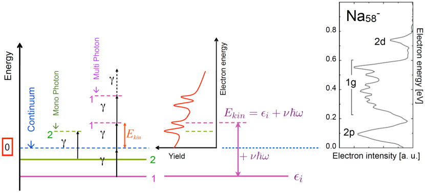
Figure 8: Left : schematic view of photoelectron spectroscopy (PES), including multiphoton ionization scenario for the most bound state. The sample system has two single electron states, $\epsilon_{1}<\epsilon_{2}<0$. The emission threshold is taken as the reference of zero energy, here the ionization potential IP$=-\epsilon_{2}$. The measured kinetic energies of emitted electrons are then recorded from threshold on upwards involving a varying number $\nu$ of photons which produces successive copies of the single electron energies, separated by the laser frequency. Right : experimental example of PES measurement for the ${{\rm Na}_{58}}^{-}$ cluster (monophoton regime), obtained with photons of energy 4.02 eV [46].

A hypothetical system with two accessible valence states is considered (levels 1 and 2) whose electrons can reach the continuum via 1 or 2 photon absorption. In the multiphoton case, the resulting PES displays copies of the original PES, separated by the laser frequency. The PES is furthermore illustrated on an experimental example (right part) from ${{\rm Na}_{58}}^{-}$, in the monophoton case. The case of anionic clusters is emblematic of one-photon PES. Indeed, in such clusters, valence electron states are little bound so that they can easily be turned to continuum electrons according to Eq. (9) with one photon in the visible. These measurements basically provide a structural information on the system. In the present case, the PES exhibits well resolved peaks associated to the single electron states, as indicated in standard spectroscopic notation. One can note that the degeneracy of the $1g$ state is split into a series of sub-peaks because of symmetry breaking of the ionic configuration. Such one-photon measurements on anionic clusters were thus already performed in the early 1990’s [48]. More recent measurements nowadays allow one to access PES for neutral or even cationic clusters, as those from neutral fullerenes [16, 47] and from positively charged metal clusters [49].

MPI, as already indicated in Eq. (9) with $\nu>1$, is also possible thanks to the high coherence of laser pulses. The impact on PES will be discussed at length in Secs. 4.3.3 and 4.3.4. Let us however give a few words here. For moderate laser intensities, the MPI maps in the PES further copies of the occupied electron spectrum with increasing kinetic energy, each copy separated by $\hbar\omega_{\rm las}$. For larger intensities, the regular pattern of copies of the single electron spectrum is blurred because of large ionization affecting the spectrum itself. At even higher intensities the signal mostly becomes exponential with basically no structure left [15, 50].

Fig. 9 shows a typical example of a PES measurement, in this case performed on cationic species.

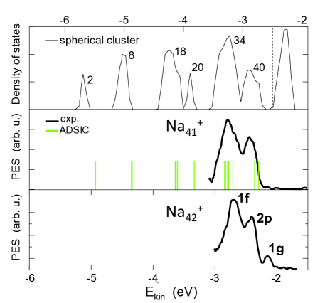
Figure 9: Lower and middle panels: Experimental photoelectron spectra for ${{\rm Na}_{41}}^{+}$ (bottom) and ${{\rm Na}_{42}}^{+}$ (middle) obtained by irradiation from an ArF^- excimer laser of frequency $\hbar\omega_{\mathrm{las}}$ = 6.42 eV [49]. Vertical lines in the middle panel : static Kohn-Sham single particle energies of ${{\rm Na}_{41}}^{+}$ calculated in ADSIC. Upper panel: Kohn-Sham density of states for a spherical neutral Na₄₀ calculated in LDA [51].

The chosen material is sodium in which it is well known that electronic shell closure leads to especially stable configurations [10]. In turn, the PES is expected to display the corresponding shell structure. The figure focuses on the region of 40 electrons (which corresponds to a shell closure). For comparison, the expected shell sequence, as computed in the Clemenger-Nilsson approach [11], is indicated in the upper panel. Note that in that case only the two least bound shells altogether containing 20 electrons were measured. The figure exhibits several interesting features. First the comparison between ${{\rm Na}_{41}}^{+}$ and ${{\rm Na}_{42}}^{+}$ (which contains 41 electrons) very clearly points out the shell closure at 40 electrons with the appearance of one single electron in the 1g level around 5.2 eV. This also complies with the expected level sequence displayed in the upper panel. Finally, for the sake of completeness, we have also indicated the results of a DFT calculation performed with the ADSIC correction (see section 3.2 for details). The agreement obtained without any adjustment is remarkable. It should nevertheless be noted that in that case the PES mostly provides a structural information on the system by giving access to the sequence of energies of occupied single electron levels. As we shall see below, PES, especially in the MPI regime, can also provide valuable information on the dynamics of the electron cloud.

As a first example of study of electron dynamics by PES, an example on which we shall come back later (see section 4.5.2), we consider the case of C₆₀ irradiated by laser pulses of various fluences, but fixed pulse duration of 150 fs [47], see Fig. 10.

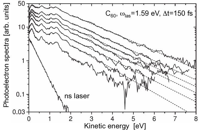
Figure 10: Photoelectron spectra of C₆₀ irradiated by a laser of frequency of 1.59 eV, pulse duration of 150 fs, and various fluences of (from top to bottom) 2.19, 1.84, 1.70, 1.56, 1.42, 1.27, and 1.13 J/cm². Adapted from [47].

At variance with the spectroscopic character of the PES in Fig. 9, the PES presented here display an almost monotonous exponential shape with little structures on top. The latter structures are interpreted as signals from single-photon ionization of Rydberg states [16]. The exponential slope is explained as reflecting thermal electron emission [52]. In this picture, the energy deposited by the laser is concerted into thermal electron energy. Concluding on the nature of the energy conversion on the single basis of the PES is nevertheless a bit questionable as exponential PES are also naturally obtained by considering higher and higher MPI processes [50]. On the other hand, the experiments of [47] also measured the PAD of emitted electrons and clearly identified a strong isotropic component which might indeed be associated to thermal emission. The interpretation of [47] is thus certainly to be considered very seriously. We shall come back on that point in Sec. 4.5.2 when discussing effects of dissipation on electronic observables in more detail. At present stage, it is sufficient to conclude that PES clearly opens the door to the analysis of electron dynamics. And that PAD offers for sure an invaluable complement to such studies (see next section 2.3.2).

Finally, and before discussing PAD we would like to discuss another possible application of the PES now involving rather long time scales. Fig. 11 shows an example of a time-resolved photoelectron spectrum (TRPES) measured in (H₂O)${}_{30}^{-}$ [53].

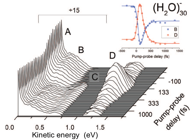
Figure 11: Time-resolved photoelectron spectra of (H₂O)${}_{30}^{-}$ irradiated by a pump of 1.00 eV and a probe of 1.57 eV. The spectrum below 1 eV has been multiplied by 15. See text for the explanation of the features A, B, C and D. Inset: integrated intensity of features B and D as a function of pump-probe delay. From [53].

The irradiation process is performed with a pump-and-probe setup of laser frequencies of 1 and 1.57 eV respectively, and similar intensities (50-100 $\mu$J per pulse). The PES exhibit a clear dependence on the delay between the pump and the probe. The four major structures are indicated by capital letters. The low energy structure (A) is associated to excited-state autodetachment, while direct probe detachment from the ground state (B) is observed around 0.25 eV. Structure around 0.6 eV (C) is attributed to resonant two-photon detachment from the pump , and finally transient excited-state signal (pump-probe, D) appears in the 1.00–1.50 eV kinetic energy range. Integrating the intensities of these structures provides the associated population dynamics, which is indicated in the inset of Fig. 11 for structures (B) and (D). Both exhibit a similar decay time. To summarize, the above result clearly shows that a TRPES provides an extremely rich tool of investigation of details of electron dynamics. Such measurements, possibly complemented by theoretical investigations, should thus help to reveal crucial information on irradiation scenarios. Even more so PAD bring an invaluable complement to PES, as we shall see in the next section.

2.3.2 Photo-Angular Distributions (PAD) and PES/PAD

Photo-Angular Distributions bring an invaluable complement to Photo-Electon Spectra. An example of PAD is shown in Fig. 12, adapted from [17].

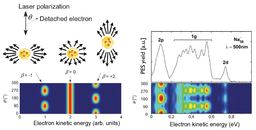
Figure 12: Top left : schematic view of various types of photoemission distributions (from left to right : oblate, isotropic, and prolate). Bottom left : ideal photoangular distributions corresponding to each case, with the respective value of the anisotropy parameter $\beta$. Right : experimental PES (top) and PES/PAD (bottom) of ${{\rm Na}_{58}}^{-}$ cluster, irradiated by linearly polarized pulses from a dye laser (pulse width of about 10 ns, peak intensity below 10⁵ W/cm² and photon energy 4.02 eV). Adapted from [17].

The PAD are plotted as a function of electron kinetic energies, so that they in fact represent a combined PES/PAD. The mere PAD can then be obtained by integrating over kinetic energies. It should be immediately noted that the notion of PAD requires a proper definition of a reference frame. The reference direction is given by the laser polarisation axis and angular distributions are thus measured with respect to this axis. But it should also be noted that, in the gas phase, the actual orientation of clusters or molecules with respect to this polarisation axis is unknown so that one has at best access to an orientation averaged (of the molecule with respect to the laser polarisation) signal. This in particular reduces the angular distribution to a dependence on the angle between the laser polarization axis and the detection angle, because of angular averaging around the polarization axis. For then, in the case of single photon absorption, the cross section takes the simple form :

$$\frac{\textrm{d}\sigma}{\textrm{d}\Omega}\propto 1+\beta_{2}P_{2}\left(\cos\theta\right)\quad,$$ (10)

where $\theta$ is the direction of the emitted electron measured with respect to the laser polarisation, $P_{2}$ is the second order Legendre parameter and $\beta_{2}$ is known as the anisotropy parameter. In the simple case of one photon processes, the angular distribution is thus fully characterised by the anisotropy parameter $\beta_{2}$ which takes values between -1 and 2. Three values of $\beta_{2}$ are thus special, as illustrated in the left part of Fig. 12 : $\beta_{2}$=2 corresponds to a prolate-like form of the (orientation averaged) emission cloud along the laser polarisation, so that signal will gather around 0^∘ and 180^∘; $\beta_{2}$=-1 corresponds to a purely transverse emission, oblate-like shape, with signal gathering around 90^∘ and 270^∘; finally $\beta_{2}$=0 corresponds to a fully isotropic emission.

A realistic measurement is shown in the right part of Fig. 12 to complement the schematic part. The measurement has again been performed in ${{\rm Na}_{58}}^{-}$, thus complementing the PES example of Fig. 8. We nevertheless indicate the latter PES for completeness and to ease the explanation of the features of the combined PES/PAD. As already noted in the discussion of Fig. 8, the case demonstrates a clear dependence of the photoemission on the nature of the electronic wave functions (indicated with spectroscopic notations in the figure). Comparing the PES (upper right panel) to the PES/PAD (lower right panel), one can see that the $2p$ and $2d$ electrons are emitted parallel to the laser polarization. On the contrary, the emission from all the $1g$ states occurs preferentially aligned in the transverse direction. This demonstrates that PAD certainly adds further useful information on the spatial structure of the emitting states.

Another example of PES/PAD, this time in the standard VMI presentation, is shown in Fig. 13 in the case of ${{\rm C}_{18}}^{-}$ [54].

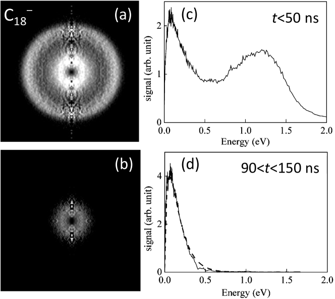
Figure 13: Velocity map images (left panels) of ${{\rm C}_{18}}^{-}$, and corresponding photoelectron spectra (right panels), after irradiation by laser pulses with frequency of 4.025 eV and duration of a few ns. Top row : yields accumulated for $t<50$ ns. Bottow row : yields accumulated for $90<t<150$ ns. Adapted from [54].

In this representation, the VMI provides a polar image of the directions (angle) and kinetic energies (radius) of the emitted electrons, again with a well defined reference axis provided by the laser polarization. The example of Fig. 13 is furthermore time-resolved, or at least allows one to separate well separated time scales of emission. Irradiation is performed with photons of frequency 4.025 eV and pulse durations in the ns range. Panel (a) provides an image of photoelectrons emitted during the first 50 ns after excitation, and the corresponding PES is plotted in panel (c). The PES exhibit two maxima, also visible as rings in panel (a), one at high energy and one at low energy. The high energy signal is associated to direct emission from the photo-excitation itself. The low energy component is attributed to thermionic emission in which the original laser energy has been partly equipartitioned between vibronic degrees of freedom of the cluster, prior to electron emission. The time scale and the typical energies associated to thermoionic emission are thus much larger than the ones associated to direct emission. In the present experiment the typical time scales of thermoionic emission lie in the tens to hundreds of ns, which in that case can be identified experimentally. The scenario is confirmed in panels (b) and (d) which present the VMI and the PES recorded in a late time window, that is between 90 and 150 ns. The PES is now fully concentrated at low energies, with no sign of a high energy, direct emission, component. This confirms the thermoionic nature of this late, low energy, emission. Therefore, even at a coarse time level, such an analysis exemplifies the capabilities of PES and PES/PAD to analyse electron dynamics in detail. We shall come back on those aspects later, see in particular Secs. 4.3, 4.4 and 4.5.

3 Theoretical approaches

Many-particle systems such as molecules or clusters, are highly correlated, and exact calculations of their properties are extremely involved, mostly beyond feasibility for finite systems without major symmetries. The main issue concerns here the treatment of electrons. Except for some specific cases, ions can be treated as classical particles. This will always be the case in the following. To deal with the electronic problem, a variety of approaches has been developed, each one being a compromise between precision and expense. In this section, we present the most widely used schemes, paying a particular attention to density-functional theory (DFT) which is one of the most efficient tools in cluster dynamics.

Before going into details of the theoretical treatment, we schematically summarize in Fig. 14 the most widely used theoretical approaches and sketch the regimes of their applicability in a plane of excitation energy and particle number.

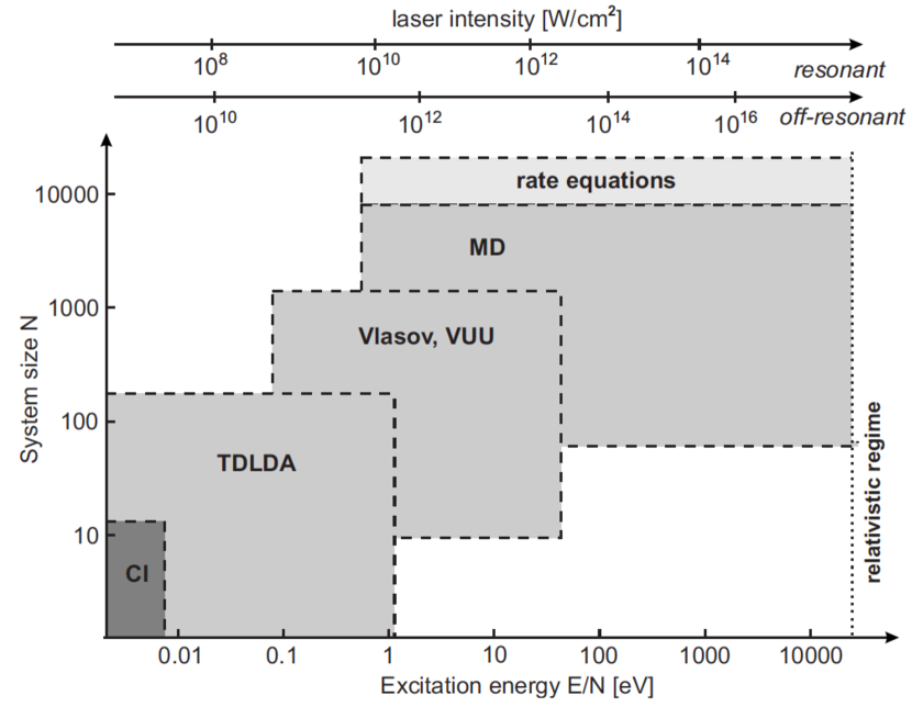
Figure 14: Schematic view of applicability of different approaches (see text for details) in a landscape of system size versus excitation energy per atom. The excitation energy can be loosely related to typical laser intensities in the optical range. This is indicated by the intensity scales on top, which are, however, also strongly dependent on the response of the particular system, i.e. resonant or non-resonant.

The boundaries of the regimes are to be understood as very soft with large zones of overlap between the models because the choice of a method also depends on several aspects (e.g., demand on precision, material, time span of simulation). The most elaborate models are the “ab-initio” methods which deal in a systematic manner with a Hamiltonian as exact as possible. The simplest example is the Hartree-Fock approximation which, however, misses the crucial electronic correlations. A typical example of the more elaborate approaches is the Configuration Interaction (CI) method which relies on an expansion of the exact many-body wave function into a superposition of Slater states [55, 56]. The limitations for CI (and other ab-initio methods) are purely a matter of practicability. The limitation is nevertheless even more severe for dynamical applications of such theories, which are thus presently restricted to rather small system sizes and small excitation energies. The range of applicability will slowly grow with the steadily increasing computer power. Density functional theory (DFT) describes a system effectively in terms of a set of single-electron states (see Sec. 3.1.2). It is limited in system size for practical reasons and in excitation energy for physical reasons, because of the missing dynamical correlations from electron-electron collisions. Nevertheless, DFT and even more so its time dependent extension TDDFT (especially when realized in full real time) nevertheless provide a most robust and versatile tool in the field. A semi-classical mean-field description is provided by the Vlasov equation originally designed for plasma physics [57]. This approach ignores quantum effects such as shell structure or tunneling and thus becomes questionable at low energies. It is furthermore reasonably tuned to metal electrons because of their ressemblance to a Fermi gas, but more difficult to apply in other materials, especially in covalent bound systems. On the other hand, the semi-classical treatment allows one to include dynamical correlations due to electron-electron collisions, leading to the Vlasov-Uehling-Uhlenbeck (VUU) approach [58, 59, 60], which extends the applicability to larger energies than those allowed by TDLDA. Even higher excitations and system sizes are the realm of electronic Molecular Dynamics approaches and rate equations which, however, are even more limited than VUU for low energies and small systems [61]. The upper limit in energy is given by the onset of the relativistic regime, where retardation effects within the coupling begin to severely influence the dynamics.

In the following, we shall use real-time TDDFT as the basic theory to describe ionization dynamics. We shall occasionally use VUU in order to discuss electronic temperature effects, as observed in some experiments. We thus briefly describe in this section basics of TDDFT and practical implementations thereof. We discuss in some detail the self-interaction correction strategy to be developed to properly account for ionization in a dynamical way within standard approximations of DFT. We next present in detail the tools developed to access PES and PAD in TDDFT. We in particular discuss the demanding inclusion of orientation effects of the irradiated clusters and molecules with respect to laser polarization. We finally remind basics of VUU for completeness.

3.1 Basic formalism

3.1.1 Handling of the ionic background

The interaction between the ions in a cluster and the electrons is usually described by pseudopotentials. This allows one to eliminate the inert, deep lying electron states around each ion and to concentrate on the relevant valence electrons. For a detailed discussion of pseudopotentials see, e.g., [62]. We go here a pragmatic way and take published pseudopotentials. For simple metals, we consider the soft, local pseudopotentials of [63]. In more general cases, we employ mostly the local and non-local pseudopotentials in separable form as introduced in [64]. More precisely, for each type of atom with $Z$ valence electrons, we use the pseudopotential $V_{\mathrm{PsP}}$ of the following form :

$$V_{\mathrm{PsP}}(\mathbf{r})\,\varphi_{j}(\mathbf{r}) = V_{\mathrm{loc}}(r)\,\varphi_{j}(\mathbf{r})+\int\textrm{d}^{3}\mathbf{r}^{\prime}\,V_{\mathrm{nloc}}(\mathbf{r},\mathbf{r}^{\prime})\,\varphi_{j}(\mathbf{r}^{\prime})\;,$$ (11a)

$$V_{\mathrm{loc}}(r) = -\frac{Z}{r}\,{\rm erf}\left(x/\sqrt{2}\right)+\exp\left(-x^{2}/2\right)\left[C_{1}+C_{2}\,x^{2}\right],\;x=\frac{r}{r_{\mathrm{loc}}}\;,$$ (11b)

$$V_{\mathrm{nloc}}(\mathbf{r},\mathbf{r}^{\prime}) = p(r)\,h_{0}\,p(r^{\prime})\;,$$ (11c)

$$p(r) = \frac{\sqrt{2}}{{r_{\mathrm{nloc}}}^{3/2}\sqrt{\Gamma\left(3/2\right)}}\exp\left(-\frac{r^{2}}{2{r_{\mathrm{nloc}}}^{2}}\right)\;.$$ (11d)

Here $\varphi_{j}$ denotes the wave function of state $j$, ${\rm erf}$ the error function, $\Gamma$ the Gamma function, and $x=r/r_{\mathrm{loc}}$. The refitted parameters are $C_{1}$, $C_{2}$, $r_{\mathrm{loc}}=r_{\mathrm{loc}}$, and $h_{0}$. The standard parameters are given in [64]. However, for the results presented in Section 4, we use often refitted parameters which employ larger radii $r_{\mathrm{loc}}$ and $r_{\mathrm{nloc}}$, thus softer pseudopotentials for more robust numerical handling, see Section 3.1.3.

There also exists a commonly used alternative to pseudopotentials for metallic systems. In particular, simple metals have valence electrons with long mean free path throughout. The fine details of the ionic background can thus be seen by the electrons only in an average manner. This motivates the jellium approximation in which the ionic background is smeared out to a constant positive background charge. This is a standard approach in bulk metals [65]. It has been generalized to finite clusters. In its simplest form, one carves from the bulk a finite, homogeneously and positively charged sphere of radius $R=r\,N_{\mathrm{ion}}^{1/3}$, whose total ion charge reproduces the given ionic charge $eN_{\mathrm{ion}}$. A more flexible approach is achieved when allowing for a finite surface width, yielding the soft jellium model

$$\rho_{\mathrm{jel}}(\mathbf{r})=\frac{3}{4\pi r_{s}^{3}}\left[1+\exp\left(\frac{|\mathbf{r}|-R_{\mathrm{jel}}}{\sigma_{\mathrm{jel}}}\right)\right]^{-1}\quad,$$ (12)

with $R_{\mathrm{jel}}$ being defined by normalization to the total particle number $\int\textrm{d}^{3}\mathbf{r}\,\rho_{\mathrm{jel}}=N_{\mathrm{ion}}.$ The central density reproduces the bulk density $\rho_{0}={3}/({4\pi r_{s}^{3}})$. The parameter $\sigma_{\mathrm{jel}}$ accounts for a smooth surface transition from $\rho_{0}$ to zero. The surface width (transition from 90% to 10% bulk density) is about $4\sigma_{\mathrm{jel}}$. The model can be extended to also describe deformations which can have a considerable influence in metal cluster spectroscopy depending on the system [66, 67].

3.1.2 Density Functional Theory and its Time-Dependent version

The goal of DFT is to develop self-consistent equations which employ effective potentials for the contributions from exchange and correlation. These potentials are to be expressed in terms of the total local electron density $\rho(\mathbf{r})$ of the system. The success of DFT depends on a diligent choice of these effective potentials. For the brief review of DFT, we take here a practitioners approach and discuss the Kohn-Sham (KS) scheme from a given energy functional. We do not address the theoretical foundations of DFT in terms of the much celebrated Hohenberg-Kohn theorem [68] and Kohn-Sham formalism [69]. The many aspects of foundation and derivation can be found, e.g., in [70, 71, 72].

3.1.2.1 The energy functional

The starting point is an energy functional for the total electronic energy $E_{\mathrm{total,el}}$. In the Kohn-Sham (KS) scheme, one represents the $N$ (valence) electrons, by $N$ non-interacting Kohn-Sham (KS) orbitals (or s.p. states) $\varphi_{i}(\mathbf{r})$, $i\in\{1,\ldots,N\}$. The total energy is then separated into kinetic energy (which then takes a simple form) and interaction energy (associated to the above mentioned effective pseudopotentials). The total electronic density is expressed from the KS orbitals as :

$$\rho(\mathbf{r})=\sum_{i=1}^{N}\big{|}\varphi_{i}(\mathbf{r})\big{|}^{2}\quad.$$ (13)

Note that DFT schemes allow one to treat spin-up and spin-down density separately. For simplicity of presentation, we drop the spin dependence in the following. The total electronic energy is then composed as

$$E_{\mathrm{total,el}}[\rho] = E_{\mathrm{kin}}(\{\varphi_{i}\})+E_{\mathrm{H}}[\rho]+E_{\mathrm{xc}}[\rho]+E_{\mathrm{coupl}}+E_{\mathrm{ext}}\quad,$$ (14a)

$$E_{\mathrm{kin}}\left(\{\varphi_{i}\}\right) = -\frac{\hbar^{2}}{2m}\ \int\textrm{d}^{3}\mathbf{r}\sum_{i=1}^{N}\varphi_{i}^{*}(\mathbf{r})\ \nabla^{2}\ \varphi_{i}(\mathbf{r})\quad,$$ (14b)

$$E_{\mathrm{H}}[\rho] = \frac{e^{2}}{2}\iint\textrm{d}^{3}\mathbf{r}\ \textrm{d}^{3}\mathbf{r}^{\prime}\ \frac{\rho(\mathbf{r})\rho(\mathbf{r}^{\prime})}{|\mathbf{r}-\mathbf{r}^{\prime}|}=\frac{1}{2}\int\textrm{d}^{3}\mathbf{r}\ \rho(\mathbf{r})\ U_{\mathrm{H}}[\rho]\quad,$$ (14c)

$$E_{\mathrm{coupl}} = \int\textrm{d}^{3}\mathbf{r}\,\sum_{i=1}^{N}\varphi_{i}^{*}(\mathbf{r})\ \hat{V}_{\mathrm{coupl}}\ \varphi_{i}(\mathbf{r})\quad,$$ (14d)

$$E_{\mathrm{ext}} = \int\textrm{d}^{3}\mathbf{r}\ \rho(\mathbf{r})\ U_{\mathrm{ext}}(\mathbf{r})\quad.$$ (14e)

The kinetic energy is a functional of the s.p. orbitals $\varphi_{i}$ which serves to maintain the quantum shell structure in the KS calculations. The non-trivial correlation part of the exact kinetic energy is summarized in the interaction energy. The interacting term is mapped to the density functionals $E_{\mathrm{H}}[\rho]+E_{\mathrm{xc}}[\rho]$. The first term $E_{\mathrm{H}}$ is the standard (direct) Coulomb Hartree energy, which naturally is a functional of $\rho$. We have introduced here the notation $U_{\mathrm{H}}$ for the corresponding Hartree potential. Conceptually simple are $E_{\mathrm{coupl}}$ from the coupling to the ions ($\hat{V}_{\mathrm{coupl}}$ is the potential operator built from the pseudopotentials) and the energy $E_{\mathrm{ext}}$ modeling an external electromagnetic field $U_{\mathrm{ext}}(\mathbf{r})$. Both these contributions couple to single electrons and are naturally well represented by an independent particle picture in terms of $\varphi_{i}$.

Finally, there is the exchange-correlation energy $E_{\mathrm{xc}}$ which accumulates all pieces of the exact energy not yet accounted for. This is the most problematic part in the scheme, since its functional expression is not exactly known. Many approximations thereof do exist, among which the simplest and most robust one is the Local Density Approximation (LDA). The construction of LDA is simple. One computes the ground state of the homogeneous electron gas as exactly as possible and obtains the exchange-correlation energy per volume $E_{\mathrm{xc}}/V=\rho\,\epsilon_{\mathrm{xc}}(\rho)$. Here this energy is still a function of the (homogeneous) density $\rho$. The crucial point is to allow now for an inhomogeneous, and time-dependent if needed, density $\rho(\mathbf{r},t)$ in that expression. It amounts to considering the energy as composed piecewise from an infinite electron gas of densities $\rho(\mathbf{r},t)$ which is a bold approximation. Nonetheless, LDA provides a robust description for a wide variety of systems. There is an enormous body of literature pondering successes and failures, for a more detailed discussion, see e.g. [71]. Note that a functional depending on $\rho(\mathbf{r},t)$ employs the instantaneous density and thus excludes any memory effect. This time-dependent generalization is often called adiabatic LDA (ALDA). Again, we use in the following the generic notation LDA.

The validity of LDA depends very much on the system under consideration. One of the major problems is the self-interaction error : the single particle state $\varphi_{i}$ is included in the density $\rho$, and thus contributes to the mean-field Hamiltonian $\hat{h}_{\mathrm{KS}}$ (see Eq. (15b) below) which acts on $\varphi_{i}$. This yields a wrong asymptotics for the Coulomb mean field. For example, for a neutral system described in LDA, it decays exponentially at large distances instead of $\propto e^{2}/r$ as it should. An attempt to reduce the self-interaction error is the generalized-gradient approximation (GGA) which augments LDA with an additional dependence on $\nabla\rho$ [73, 74]. GGA yields a significant improvement in the computation of atomic and molecular binding. For example, it lifts the description of dissociation energies to a quantitative level. However, GGA does not fully remove the self-interaction error. Thus there are various attempts for further improvement as, e.g., adding kinetic terms to DFT [75]. Another line of development is to explicitly implement a Self-Interaction Correction (SIC). This helps to deliver correct ionization properties, which is crucial in describing PES and PAD dynamically. We will therefore discuss this approach in more detail in Sec. 3.2.

As indicated above, time-dependent DFT, effectively using ALDA, makes also an adiabatic approximation. In order to account for dynamical effects, a Current DFT (CDFT) has been developed, which is based on LDA augmented by a dependence on electronic currents evaluated in the linear response [76, 77, 78]. The response kernels in the extended functional include memory effects and allow one to describe relaxation [79]. CDFT is rather involved and thus there exist so far only applications to symmetry restricted systems as, e.g., in solids[80]. The underlying linear response modeling makes CDFT an extension for low excitation energies and/or amplitudes. Real electron-electron collisions become important for more energetic processes. These are often treated by a quantum generalization of the Boltzmann collision term. We will address this extension of DFT in Secs. 3.5 and 5.2.

3.1.2.2 The Kohn-Sham equations

The stationary KS equations are derived by variation of the total energy with respect to the s.p. wave functions $\varphi_{i}^{*}$, yielding :

$$\hat{h}_{\mathrm{KS}}[\rho]\ \varphi_{i}(\mathbf{r}) = \varepsilon_{i}\ \varphi_{i}(\mathbf{r})\quad,$$ (15a)

$$\hat{h}_{\mathrm{KS}}[\rho] = -\frac{\hbar^{2}\nabla^{2}}{2m}+U_{\mathrm{KS}}[\rho]+\hat{V}_{\mathrm{coupl}}+U_{\mathrm{ext}}\quad,$$ (15b)

$$U_{\mathrm{KS}}[\rho] = U_{\mathrm{H}}[\rho]+U_{\mathrm{xc}}[\rho]\quad.$$ (15c)

The local and density-dependent Kohn-Sham potential $U_{\mathrm{KS}}$ consists in the direct Coulomb term $U_{\mathrm{H}}$ and the exchange-correlation potential, which is a standard functional derivative $U_{\mathrm{xc}}=\delta{E}_{\mathrm{xc}}/\delta\rho$. Coupling potentials to ions and to the external field are trivially given.

The time-dependent KS equations analogously read :

$${\rm i}\hbar\ \partial_{t}\varphi_{i}(\mathbf{r},t)=\hat{h}_{\mathrm{KS}}[\rho]\,\varphi_{i}(\mathbf{r},t)\quad,$$ (16)

where $\hat{h}_{\mathrm{KS}}$ is composed in the same manner as above, provided that one replaces $\rho(\mathbf{r})$ by $\rho(\mathbf{r},t)$. This assumes an instantaneous adjustment of the total electronic density, although memory effects can play in some cases an important role, especially in $E_{\mathrm{xc}}$ [72].

The stationary KS equations (15a) pose an eigenvalue problem. They provide the electronic ground state of a system. This is a highly non-linear problem due to the self-consistent feedback of the local density in the KS hamiltonian. It is usually solved by iterative techniques [14]. The time-dependent KS equations imply an initial value problem. The natural starting point is the ground state obtained from the stationary KS equations. The time-dependent KS system can then be solved by standard methods of first order differential equations [14]. We finally remind that we wrote spinless KS equations. One can easily include the electron spin in Eqs. (15). We refer the reader to [70, 71, 72] for more details.

3.1.3 A few words on numerical implementation

A representation of the s.p. wave functions $\varphi_{\alpha}(\mathbf{r},t)$ and the fields $\rho(\mathbf{r},t)$ and $U_{\mathrm{KS}}(\mathbf{r},t)$ on a coordinate-space grid is strongly recommended if one aims at computing electronic emission properties. Conceptually straightforward is a Cartesian 3D grid with equally spaced mesh points. This leaves two choices for the description of the kinetic energy, that is finite difference schemes [81, 82, 83, 84] or the Fourier definition exploiting the extremely efficient fast Fourier transformation (FFT) [85, 86, 14]. The Coulomb problem is solved either by iterative methods (e.g., successive over-relaxed iterations) in connection with finite-difference schemes or by Fourier techniques in case of FFT. In the latter case, one can produce an exact solution on the grid by using a double grid (in each direction) [87] or, somewhat faster, by eliminating the long-range terms by a separate analytical treatment [88]. A fast scheme for the static solution is provided by the damped gradient iteration [89]. The scheme for time evolution depends on the representation of the kinetic energy. For finite-difference schemes, one typically uses a second order predictor-corrector with a Taylor expansion of the KS time-evolution operator while for FFT schemes, the time-splitting (also called $\hat{T}$-$\hat{V}$ splitting) technique is preferable in connection with the FFT representation [90]. An extensive comparative study of the various griding and iteration techniques can be found in [91].

Let us end with a few words in the case of symmetric systems. For instance, the jellium model allows a description in higher symmetry, that is a representation on an axial 2D grid [92]. In the case of explicit ions in simple metal clusters, they can be described by soft, local pseudopotentials. This allows an averaging over axial angle, leading to the cylindrically averaged pseudopotential scheme (CAPS) [93] which is extremely efficient and thus has been used in many explorative studies. The CAPS allows one to treat explicit ionic structure in full 3D with pseudopotentials while keeping electrons with cylindrical symmetry [14]. This turns out to be a very good approximation for metals and it is even exact for linear molecules such as carbon chains [94]. It has even allowed to step forth to rather complex systems as, e.g., embedded clusters [95, 96]. The Fourier representation of kinetic energy cannot be applied in this geometry. Finite differences are the method of choice in axial grids. The static solutions use the same iterative schemes as in 3D. A particularly suitable time-stepping scheme for axial 2D is the Peaceman-Rachford step, which is a separable version of the well known Crank-Nicholson step [97, 98].

3.2 The self-interaction problem in DFT and TDDFT

As outlined above, LDA is plagued by the self-interaction error which is particularly harmful for ionization properties. The safest way to deal with that is to introduce an explicit Self-Interaction Correction (SIC). A conceptually simple and robust SIC was introduced by J. Perdew and A. Zunger in which all single-particle self-interactions are subtracted from the DFT energy [99] :

$$E_{\mathrm{SIC}}[\rho]=E_{\mathrm{LDA}}[\rho]-\sum_{\alpha=1}^{N}E_{\mathrm{LDA}}[\rho_{\alpha}]\quad,\quad\rho_{\alpha}(\mathbf{r})=\left|\psi_{\alpha}(\mathbf{r})\right|^{2}\quad,$$ (17)

where $E_{\mathrm{LDA}}=E_{\mathrm{H}}+E_{\mathrm{xc}}$ is the LDA functional for the Coulomb-Hartree term as well as exchange and correlations. Note that we have changed here our standard notation for the single electron KS orbitals from $\varphi_{i}$ to $\psi_{\alpha}$. This is done on purpose as will become clear below in Eq. (20). The self-interaction corrected KS equations are then derived again by variation. A problem is that the emerging SIC-KS hamiltonian $\hat{h}_{\mathrm{SIC}}$ then becomes state-dependent because $\delta{E}_{\mathrm{LDA}}[\rho_{\alpha}]/\delta\psi_{\beta}^{*}\propto\delta_{\alpha\beta}$ is state selective. We formulate this in terms of a projector and obtain :

$$\hat{h}_{\mathrm{SIC}} = \hat{h}_{\mathrm{LDA}}-\sum_{\alpha}U_{\alpha}|\psi_{\alpha}\rangle\langle\psi_{\alpha}|\quad,\quad U_{\alpha}=\frac{\delta{E}_{\mathrm{LDA}}[\rho_{\alpha}]}{\delta\rho_{\alpha}}\quad.$$ (18)

It becomes apparent that the state dependence leads to a non-Hermitian SIC hamiltonian. This leads to a violation of orthonormality of the $\psi_{\alpha}$. To restore it, we have to add a constraint $\sum_{\alpha\beta}\lambda_{\alpha\beta}\langle\psi_{\beta}|\psi_{\alpha}\rangle$ to the SIC energy with the (hermitian) Lagrange multiplier $\lambda_{\alpha\beta}$. The SIC mean-field equations thus become :

$$\hat{h}_{\mathrm{SIC}}|\psi_{\alpha}\rangle=\sum_{\beta}\lambda_{\beta\alpha}|\psi_{\beta}\rangle$$

for the static case and

$$\left(\hat{h}_{\mathrm{SIC}}-\mathrm{i}\hbar\partial_{t}\right)|\psi_{\alpha}\rangle=\sum_{\beta}\lambda_{\beta\alpha}|\psi_{\beta}\rangle$$

for the dynamic case. In both cases, these equations have to be complemented by the ”symmetry condition”

$$\langle\psi_{\beta}|U_{\mathrm{\beta}}-U_{\rm\alpha}|\psi_{\alpha}\rangle=0$$ (19)

which is the crucial ingredient in the scheme stemming from the orthonormality constraint [100, 101]. These SIC equations are hard to solve directly in the static case and near to impossible in dynamics. The key to success is to introduce a second s.p. basis set $\{\varphi_{l},l=1,\ldots,N\}$ which is connected to the set $\{\psi_{\alpha},\alpha=1,\ldots,N\}$ by a unitary transformation [102]

$$|\varphi_{j}\rangle=\sum_{\alpha=1}^{N}u_{j\alpha}\,|\psi_{\alpha}\rangle$$ (20)

tuned to diagonalize the matrix of $\lambda_{\beta\alpha}$. This simplifies the static and dynamic SIC-KS equations to

$$\hat{h}_{\mathrm{SIC}}|\varphi_{j}\rangle=\varepsilon_{j}|\varphi_{j}\rangle\;,\;\left(\hat{h}_{\mathrm{SIC}}-\mathrm{i}\hbar\partial_{t}\right)|\varphi_{j}\rangle=0\;.$$ (21)

Eqs. (18–21) formulate the SIC problem in the “2setSIC” scheme. They are solved by interlaced iterations. One performs a step of static or dynamics mean-field problem (21) and then adjusts the unitary transformation (20) to accomodate the symmetry condition (19). A detailed representation of the scheme can be found in [102, 100].

Although we dispose with 2setSIC of a powerful technique to solve the static and dynamical equations with SIC, it remains a tedious task. There are several interesting simplifications around. With the help of the optimized effective potential method (OEP) [103], one has developed implementations of SIC in terms of state-independent local potentials, which lead to the Krieger-Li-Iafrate (KLI) method [104] and, one step simpler, to the Slater approximation to SIC [105] (for a detailed discussion in connection with clusters, see [106]). Metal clusters are special in the sense that their valence electrons have all very similar spatial extension and stay close in energy (see for instance the s.p. energies of ${\mathrm{Na}_{41}}^{+}$ in Fig. 1). This allows one to replace the detailed $N$ s.p. densities $\rho_{\alpha}$ in SIC by a single averaged representative $\bar{\rho}_{1e}=\rho/N$ which then defines the energy functional for Average-Density SIC (ADSIC) as :

$$E_{\mathrm{ADSIC}}(\rho)=E_{\mathrm{LDA}}^{\mbox{}}(\rho)-N\,E_{\mathrm{LDA}}^{\mbox{}}(\rho/N)\;.$$ (22)

ADSIC is simple, robust, and reliable. It provides the correct asymptotics of the KS field while it is formally as simple to handle as LDA. The correct asymptotics and simplicity renders ADSIC very useful in calculating electron emission and its observables. Most examples in this article were computed with ADSIC. Although motivated by metal electrons, ADSIC also performs surprisingly well for covalent molecules, see [107, 108] and Fig. 15. Within ADSIC, the concept of s.p. densities is not needed anymore such that ADSIC is also applicable to semi-classical schemes [106]. In fact, it was first proposed by Fermi [109] in a semi-classical context.

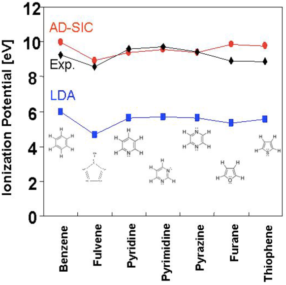
Figure 15: Ionization potentials calculated from the energy of the HOMO, for a selection of conjugated molecules. Compared are results from LDA and ADSIC with experimental data. Adapted from [107].

Fig. 15 demonstrates the effect of ADSIC for a couple of basic organic molecules. Ionization potentials (IP) presented in this figure have been computed using the energy of the Highest Occupied Molecular Orbital (HOMO) obtained from the ground state configuration of each system. The wrong asymptotic Coulomb Kohn-Sham potential of pure LDA leads to less binding and thus to much reduced IP. The deviation is uncomfortably large. Correcting the self-interaction error even with the simple ADSIC suffices to obtain a very satisfying reproduction of the experimental IP.

Fig. 16 demonstrates the effect of SIC in more detail.

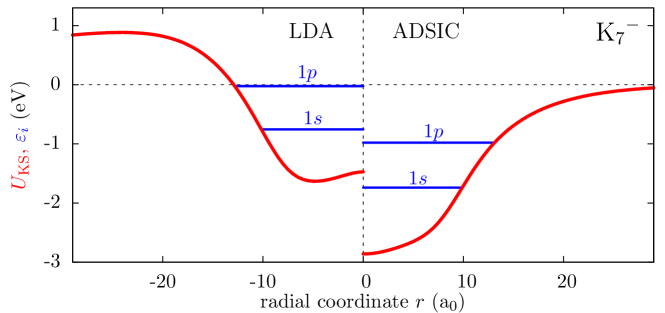
Figure 16: Kohn-Sham potential and single particles energies for ${{\rm K}_{7}}^{-}$ described with spherical jellium background. Compared are results from LDA (left) with those from ADSIC (right).

As test case, we consider the cluster anion ${{\rm K}_{7}}^{-}$ where the failure of LDA is particularly apparent. We use here a spherical soft jellium ionic background, see Eq.(12), with a Wigner-Seitz radius $r_{s}=5$ a₀ and surface parameter $\sigma=1.4$ a₀. The cluster as a whole has a negative charge. Consequently, the total Coulomb potential as it is used in LDA has an asymptotics $\propto+{e}^{2}/r$ and produces a Coulomb barrier between inside and outside. ADSIC, on the other hand, sees asymptotically the Coulomb potential of all electrons minus the one which is departing. This is the potential of a neutral system which converges exponentially to zero from below. The different asymptotic potentials mostly lead to a global shift of the s.p. energies, while the energy differences between the occupied states are less affected. This global shift is particurlarly disastrous for this anion. The system is hardly bound with LDA, while ADSIC produces comfortable and realistic binding, although weak.

Finally, we consider an example of time-dependent SIC (TDSIC) solved in the 2setSIC framework and directly analyze the ionization dynamics of a molecule. To that end, we use a simple 1D model for a H₂ dimer molecule with a smoothed Coulomb potential [110]. It is well adapted for a consistent test of SIC [102]. The two electrons have aligned spins (triplet state) to make a non-trivial test of SIC. We work at the level of “exchange only”, so that the benchmark becomes time-dependent Hartree-Fock (computed with exact exchange). To test LDA consistently, a density functional for exchange has been developed for this 1D model within LDA. This density functional is also used as a basis for SIC [102]. As SIC has a large impact on the IP, we take the time evolution of ionization as a critical test. A result for an instantaneous boost is shown in Fig. 17.

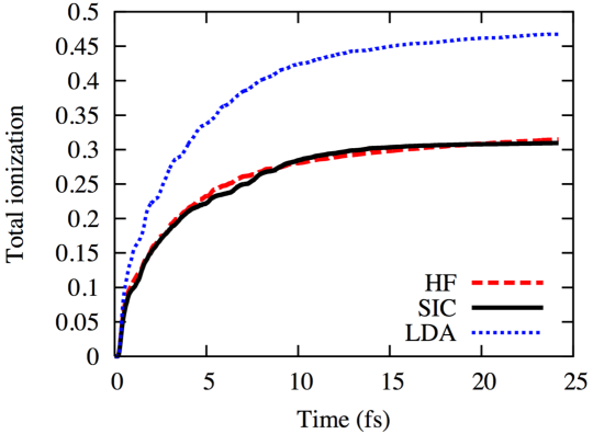
Figure 17: Time evolution of total ionization after an instantaneous boost for a 1D model of H₂ in triplet state, calculated in LDA (blue dots), Hartree-Fock (red dashes) and 2setSIC (black full curve). Adapted from [102].

The failure of TDLDA (blue dots) for this observable becomes obvious. The IP is grossly underestimated and consequently, the ionization is too high. The 2setSIC (full line) cures the problem almost perfectly, as is visible in the excellent agreement with the Hartree-Fock calculation (red dashes).

3.3 Total ionization, PES and PAD in TDDFT

In this section, we discuss detailed observables from direct electron emission. By direct emission, we mean those processes which are caused without delay by the electronic excitation process. They dominate at moderate excitations and short laser pulses with duration of some tens of fs where the competing process, that is thermalization and subsequent thermal emission, is less important. At this short time scale, we can also often neglect explicit ionic motion.

3.3.1 An example of PES and PAD as preview

As a preview, we show in Fig. 18 PES and PAD for a simple example, Na₈ with spherical jellium background. This system has only two occupied levels $1s$ (twice degenerate) and $1p$ (six-fold degenerate) which simplifies the analysis.

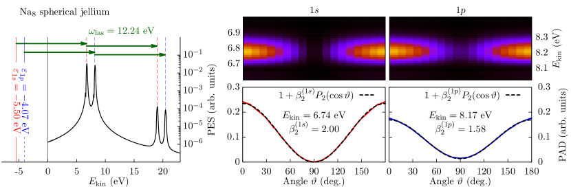
Figure 18: Photoelectron spectrum (left), photoangular distributions (bottom middle and right) and combined PES/PAD (top middle and right) from Na₈ with spherical jellium background, see Eq. (12), using $r_{s}=3.65$ a₀ and $\sigma=1$ a₀ after excitation with a linearly polarized laser pulse, see Eq. (1), of intensity $I=6.9\times 10^{13}$W/cm², frequency $\omega_{\mathrm{las}}=12.24$ eV, and pulse duration $T_{\mathrm{pulse}}=90$ fs. The two occupied s.p. states lie at $\varepsilon_{1s}=-5.5$ eV and $\varepsilon_{1p}=-4.07$ eV. The total ionization is $N_{\mathrm{esc}}=0.003$ electron. The angle $\vartheta$ is measured with respect to the laser polarization.

The left panel shows the PES, that is the distribution of kinetic energies of emitted electrons. Left of the vertical axis, the two originally occupied s.p. states are indicated. One photon adds 0.9 Ry energy and so places a peak at $-5.5+12.24$ eV, or $-4.07+12.24$ eV respectively. The energy shift by the photon is indicated by horizontal arrows. The peaks in the PES directly map the occupied states. Further 12.24 eV higher, one sees another two peaks. These are due to two-photon processes moving the electrons $2\hbar\omega_{\mathrm{las}}$ up in energy. The two upper right panels of Fig. 18 show combined PES/PAD with an energy window around the first (middle) and second (right) peaks of the PES. The lower panels show the corresponding PAD for emission from the $1s$ states (middle) and $1p$ states (right). The PAD have a very simple structure. This test case with closed electron shells and spherical jellium background is spherical throughout. The laser defines a preferred direction thus leaving axial symmetry for the process. Therefore the PAD depend only on the angle $\vartheta$ relative to the laser polarization axis. Moreover, they consist out of a constant contribution plus a cos² profile. We will see later on that this is the only possible structure for PAD from one-photon processes. The figure also indicates the anisotropy $\beta_{2}$, as defined later in Eq. (41), for each case. The PAD from a perfectly spherical $1s$ state has the maximal possible value $\beta_{2}=2$, which corresponds to strong alignment with the laser polarization and vanishing emission perpendicular to it. The less symmetrical $1p$ states yield a somewhat lower anisotropy. This simple example already demonstrates the richness of PES and PAD. It also shows that one needs get acqaueinted with technical details to better understand the content and behavior of both PES and PAD.

3.3.2 Absorbing boundary conditions

A grid representation naturally leads to reflecting or periodic boundary conditions. Reflection emerges for finite difference schemes. A representation of the kinetic energy by complex Fourier transformation is associated with periodic boundary conditions where flow leaving the box at one side is re-fed at the opposite side. Both can lead to artifacts if a sizable fraction of electronic flow hits the boundaries. There are several ways to solve the problem. The conceptually simplest approach is to enhance the size of the numerical box. However, this is not a realistic option as the expense grows cubically with the box length in 3D and quadratically in 2D. Very recently, a multi-grid method has been proposed [111] which renders the use of enlarged boxes feasible (although still at the edge of present days computer capabilities). Perfect removal of escaping particles is achieved by or exact boundary conditions [112, 113] which, again, are not yet practicable in 3D calculations. Robust and efficient are absorbing boundary conditions by an especially tailored imaginary potential [114] or by applying a mask function during time evolution [115]. The latter technique is particularly easy to implement and has been widely used in the past. Its robustness and efficiency allow one to develop advanced analyzing techniques on the grid as, e.g., the computation of PES and PAD [116]. A detailed description and discussion of this approach and its proper choice of numerical parameters is found in [117]. In the following, we will only address the mask technique for absorbing bounds.

Fig. 19 sketches the implementation of absorbing boundary conditions with computation of PES and PAD on a coordinate space grid.

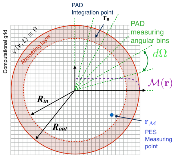
Figure 19: Schematic view of a coordinate-space grid with absorbing bounds (ring zone), a sampling direction for accumulating PAD, and measuring points $\mathbf{r}_{\mathcal{M}}$ for the PES.

Proper handling of electron emission requires absorbing boundary conditions. These are indicated by the ring area in the figure covering here 3 grid points in each direction (actual calculations typically use 6–8 points.) The absorption is performed in each time step as :

$$\varphi(\mathbf{r},t) \longrightarrow \tilde{\varphi}(\mathbf{r},t\!+\!\delta t)=\hat{\mathcal{U}}_{\mathrm{KS}}(t\!+\!\delta t,t)\,\varphi(\mathbf{r},t)\quad,$$ (23a)

$$\varphi(\mathbf{r},t\!+\!\delta t) = \mathcal{M}(\mathbf{r})\,\tilde{\varphi}(\mathbf{r},t\!+\!\delta t)\quad,$$ (23b)

$$\mathcal{M}(\mathbf{r}) = \left\{\begin{array}[]{lll}1&\mbox{for}&|\mathbf{r}|<R_{\mathrm{in}}\quad,\\ \displaystyle\cos\left(\frac{|\mathbf{r}|-R_{\mathrm{in}}}{R_{\mathrm{out}}-R_{\mathrm{in}}}\frac{\pi}{2}\right)^{\gamma_{\mathcal{M}}}&\mbox{for}&R_{\mathrm{in}}<|\mathbf{r}|<R_{\mathrm{out}}\quad,\\ 0&\mbox{for}&R_{\mathrm{out}}<|\mathbf{r}|\quad.\end{array}\right.$$ (23f)

First comes the standard step (23a) in terms of the TDLDA (or TDSIC) propagator $\hat{\mathcal{U}}_{\mathrm{KS}}$, which yields the intermediate wave function $\tilde{\varphi}(\mathbf{r},t\!+\!\delta{t})$. This is followed by the action in Eq. (23b) of the mask function $\mathcal{M}$ defined in Eq.(23f), which removes gradually any amplitude towards the bounds. We use here a spherically symmetric mask. The spherical profile is helpful to minimize griding artifacts when computing angular distributions [118]. The absorbing bounds steadily reduce the norm of the wave functions from the inner mask radius $R_{\mathrm{in}}$ to the outer one $R_{\mathrm{out}}$. The mask technique is however not perfect. One will always encounter a small amount of reflected flow, particularly for electrons with low kinetic energy. One can minimize the back-flow by proper choice of the exponent $\gamma_{\mathcal{M}}$ entering the mask profile, see Eq. (23f). This depends, however, on the actual numerics (number of absorbing points, size of time step), for a detailed discussion see [117]. Typical values of $\gamma_{\mathcal{M}}$ are of order $1/8$.

3.3.3 Ionization

The first observable which can be computed using working absorbing boundaries is the total ionization, i.e. the number of escaping electrons $N_{\mathrm{esc}}$. This can be computed simply from the, now decreasing, single-particle norms as :

$$N_{\mathrm{esc}}(t)=\sum_{i=1}^{N}N_{\mathrm{esc},i}(t)\quad,\quad N_{\mathrm{esc},i}(t)=1-\langle\varphi_{i}(t)|\varphi_{i}(t)\rangle\quad.$$ (24)

This shows that we have access to even more than the mere net ionization. Indeed each $N_{\mathrm{esc},i}$ yields the depletion of s.p. state $i$ separately. Both, total ionization and detailed level depletion are very instructive observables, see e.g. Fig. 36.

3.3.4 Photoemission angular distributions (PAD)

The angular distributions $\textrm{d}\sigma/\textrm{d}\Omega(\vartheta,\phi)$ are evaluated in angular segments labeled by the azimuthal angle $\vartheta$ and the polar angle $\phi$. The reference frame for these two angles is usually one axis, called the $z$ axis, of the Cartesian 3D grid designed to be identical with the laser polarization axis, for details see Sec. 3.4. We collect all probability which was removed by the absorption step (23b) and accumulate it. A straightforward collection of grid points in a segment tends to produce noisy results because the number of grid points per segment fluctuates. We therefore associate with each grid point a smoothing function $\mathcal{W}(\mathbf{r})$ which distributes the strength over a vicinity of order of grid spacing. This suffices to produce acceptable smooth distributions. The PAD is thus computed as :

$$\mathcal{A}(\vartheta,\phi) = \sum_{i=1}^{N}\mathcal{A}^{(i)}(\vartheta,\phi)\quad,$$ (25a)

$$\mathcal{A}^{(i)}(\vartheta,\phi) = \sum_{\mathbf{n}\in\mbox{abs.b.c.}}\int\textrm{d}r\,r^{2}\,\mathcal{W}(r\mathbf{e}_{r}-\mathbf{r}_{\mathbf{n}})\,n_{\mathrm{esc},i}(\mathbf{r}_{\mathbf{n}})\quad,$$ (25b)

$$\mathcal{W}(\mathbf{r}) = \frac{\mbox{max}(\Delta x-|x|,0)}{\Delta x}\,\frac{\mbox{max}(\Delta y-|y|,0)}{\Delta y}\,\frac{\mbox{max}(\Delta z-|z|,0)}{\Delta z}\quad,$$ (25c)

$$n_{\mathrm{esc},i}(\mathbf{r}_{\mathbf{n}}) = \int\textrm{d}t\,\left|\tilde{\varphi}_{i}(\mathbf{r}_{\mathbf{n}},t)\right|^{2}\left[1-\mathcal{M}(\mathbf{r}_{\mathbf{n}},t)\right]\quad,$$ (25d)

where $\mathbf{e}_{r}=\left(\sin\vartheta\cos\phi,\sin\vartheta\sin\phi,\cos\vartheta\right)$ is the unit vector in the direction of the wanted angles. The smoothing is done by simple tent functions which comply with the integration rule used in the normalization. The angular segments in Fig. 19 try to symbolize this smoothing which collects (weighted) information in the vicinity of a ray. The above recipe applies to state specific PAD $\mathcal{A}_{i}$ as well as the total PAD $\mathcal{A}$. Alternatively, one uses a cross-section-like notation $\textrm{d}\sigma/\textrm{d}\Omega$ for PAD. The present choice is more flexible for the presentation of orientation averaging, see Sec. 3.4.

3.3.5 Photoemission spectra (PES)

The PES can be deduced from the temporal phase oscillations of the wave functions at measuring points $\mathbf{r}_{\mathcal{M}}$ close to the absorbing bounds. This technique had been introduced in [119, 120]. A detailed discussion of the method and extension to strong laser fields is found in [121]. We summarize it here briefly. To explain the computation of PES, we first confine the considerations to 1D in order to keep things simple and extend it finally to the general 3D case. The measuring point is thus denoted for a while $z_{\mathcal{M}}$. Starting point is the solution of the Schrödinger equation for one electron in a laser field in velocity-gauge, see Eq. (4) in section 1.2.1. In this gauge, the electronic wave function $\varphi^{(v)}$ at the sampling point $z_{\mathcal{M}}$ reads

$$\varphi^{(v)}(z_{\mathcal{M}},t) = \int\frac{\textrm{d}k}{\sqrt{2\pi}}\,e^{\mathrm{i}kz_{\mathcal{M}}}\,\widetilde{\varphi}^{(v)}_{0}(k)\,e^{-\mathrm{i}\omega_{k}t+\mathrm{i}k\delta q-\mathrm{i}\delta\Omega}\quad,$$ (26a)

$$\omega_{k} = \frac{k^{2}}{2}\quad\longleftrightarrow\quad k=\sqrt{2\omega_{k}}\quad,$$ (26b)

$$\delta q(t) = E_{0}\int_{0}^{t}\mathrm{d}t^{\prime}\,F(t^{\prime})\quad,$$ (26c)

$$\delta\Omega(t) = \frac{E_{0}^{2}}{2}\int_{0}^{t}\mathrm{d}t^{\prime}\,F(t^{\prime})^{2}\quad,$$ (26d)

where $F(t)$ is the time integrated laser pulse introduced in Eq. (5). It should also be noted that Eq. (26b) exploits the fact that $z_{\mathcal{M}}$ is near the absorbing bounds, such that only outgoing waves with $k>0$ pass through this point. The aim is to deduce the momentum distribution $\left|\widetilde{\varphi}^{(v)}_{0}(k)\right|$ from the sampled $\varphi^{(v)}(z_{\mathcal{M}},t)$. This is straightforward for weak laser fields where we can neglect $\delta q$ and $\delta\Omega$. For then, a time to frequency Fourier transformation of $\varphi^{(v)}$, namely $\int\mathrm{dt}\,e^{\mathrm{i}\omega{t}}\varphi^{(v)}(z_{\mathcal{M}},t)$, produces in the right-hand side of Eq. (26a) a $\delta(\omega-\omega_{k})$ which, in turn, reduces the $k$ integration to the point $k=\sqrt{2\omega}$ thus delivering the wanted $\widetilde{\varphi}^{(v)}_{0}(\sqrt{2\omega})$.

Trying to directly apply this time-frequency transformation when the field strength is not small runs into trouble due to the non-trivial time dependencies induced by the factors $\delta q(t)$ and $\delta\Omega(t)$ in Eqs. (26). A simple solution is to counter-weight the disturbing phase factors by a phase-correction factor $e^{\mathrm{i}\Phi}$ before the transformation. We thus consider

$$\int\frac{\textrm{d}t}{\sqrt{2\pi}}\,e^{\mathrm{i}\omega t-\mathrm{i}\sqrt{2\omega}\delta q+\mathrm{i}\delta\Omega}\varphi^{(v)}(z_{\mathcal{M}},t) = \int\frac{\textrm{d}k}{2\pi}\int\textrm{d}t\,e^{\mathrm{i}kz_{\mathcal{M}}}\,\widetilde{\varphi}^{(v)}_{0}(k)\,e^{\mathrm{i}(\omega-\omega_{k})t-\mathrm{i}(\sqrt{2\omega}-k)\delta q}$$

$$\approx \int{\textrm{d}k}\,\delta(\omega-\omega_{k})e^{\mathrm{i}kz_{\mathcal{M}}}\,\widetilde{\varphi}^{(v)}_{0}(k)$$

$$= e^{\mathrm{i}\sqrt{2\omega}z_{\mathcal{M}}}\,\widetilde{\varphi}^{(v)}_{0}(\sqrt{2\omega})\quad.$$

We finally evaluate the PES yield $\mathcal{Y}_{\mathcal{M}}$ at measuring point $z_{\mathcal{M}}$ by :

$$\mathcal{Y}_{\mathcal{M}}(E_{\mathrm{kin}})\propto\left|\widetilde{\varphi}^{(v)}_{0}(\sqrt{2\omega})\right|^{2}=\left|\int\frac{dt}{\sqrt{2\pi}}\,e^{\mathrm{i}\omega t-\mathrm{i}\sqrt{2\omega}\delta q+\mathrm{i}\delta\Omega}\varphi^{(v)}(z_{\mathcal{M}},t)\right|^{2}\quad,\quad\omega\equiv E_{\mathrm{kin}}\quad.$$

The approximation here consists in assuming that the time integration, although complicated by the time profile in $\delta q(t)$, will still deliver $\omega\approx k^{2}/2$ and thus $e^{-\mathrm{i}(\sqrt{2\omega}-k)\delta q}\approx 1$. This approximation is valid anyway for weak fields. It extends the applicability of the time-frequency transformation to stronger fields. Fourier transformation of a phase-augmented wave function thus allows one to deduce the wanted momentum amplitude $\widetilde{\varphi}^{(v)}_{0}$ for a wide range of field strengths. The recipe may fail, however, for very strong fields where the temporal variation of $(\sqrt{2\omega}-k)\delta q$ dominates over $(\omega-\omega_{k})t$.

For the extension to 3D, we have to take into account that there is a whole vector of $\mathbf{k}$ rather than just two directions $k=\pm\sqrt{2\omega}$. We exploit the fact that the 3D analyzing point $\mathbf{r}_{\mathcal{M}}$ is close to the absorbing bounds (no reflection) and sufficiently far from the emitting zone. Thus the prevailing outgoing momentum $\mathbf{k}$ at this point has the direction of $\mathbf{r}_{\mathcal{M}}$, i.e.

$$\mathbf{e}_{k}=\frac{\mathbf{k}}{k}=\frac{\mathbf{r}_{\mathcal{M}}}{r_{\mathcal{M}}}=\mathbf{e}_{\mathcal{M}}\quad.$$ (27)

The frequency-momentum relation Eq. (26b) is then generalized to $\mathbf{k}=+\mathbf{e}_{\mathcal{M}}\sqrt{2\omega}$ and the PES yield at $\mathbf{r}_{\mathcal{M}}$ is identified as

$$\mathcal{Y}_{\mathcal{M}}(E_{\mathrm{kin}})\propto\left|\int\frac{\textrm{d}t}{\sqrt{2\pi}}\,e^{\mathrm{i}\omega t-\mathrm{i}\sqrt{2\omega}\delta q+\mathrm{i}\delta\Omega}\varphi^{(v)}(\mathbf{r}_{\mathcal{M}},t)\right|^{2}\quad.$$ (28)

This is the straightforward 3D generalization of the 1D formula above. The phase $\Phi(t)=-\mathrm{i}\sqrt{2\omega}\delta{q}(t)+\mathrm{i}\delta\Omega(t)$ is negligible in case of weak fields $E_{0}\ll\sqrt{\omega/2}$. It extends the applicability of the method to stronger fields.

A word is in order about the choice of gauge. The above evaluation of PES is formulated in velocity gauge because the exact solution of the Schrödinger equation in the laser field is much simpler in this gauge, see Eq. (26). If one prefers to perform numerical calculations in space gauge, one just has to apply the transformations Eq. (5) and Eq. (6) before using Eq. (28).

The effect of the phase correction in the recipe Eq. (28) is demonstrated in Fig. 20.

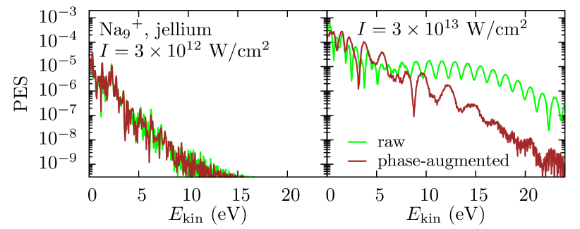
Figure 20: Ionization properties for ${{\rm Na}_{9}}^{+}$ with jellium background under the influence of a laser pulse having frequency $\omega_{\mathrm{las}}=1.4$ eV, pulse length $T_{\mathrm{pulse}}=12$ fs, and intensity as indicated in each panel. Spherical absorbing bounds were used covering at least 16 grid points. The “phase-augmented” results (brown lines) are obtained from Eq. (28), while the “raw” results (light green lines) only use the time-frequency Fourier transform of $\varphi^{(v)}(\mathbf{r}_{\mathcal{M}},t)$, see Eq. (26a) in the 1D case.

The field strength for $I=3\times 10^{12}$W/cm² is obviously sufficiently small such that there is practically no effect from the phase correction. The stronger field with $I=3\times 10^{13}$W/cm² clearly needs the phase correction and including it yields still a reliable PES. Results for significantly larger field strengths cannot be trusted.

3.3.6 Alternative routes to compute PES/PAD

An alternative theoretical approach to evaluate PES/PAD has been proposed very recently in [111]. The principle is schematically explained in the left panel of Fig. 21.

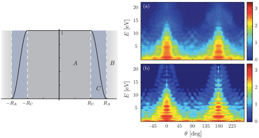
Figure 21: Example of calculated combined PES/PAD. Left : 1D view of the mask function applied in region $A$ where time-dependent Kohn-Sham equations are solved numerically in real-space, while wave functions are propagated analytically in region $B$. Region $C$ serves a a buffer region where wave functions, evaluated in $A$, overlap with those evaluated in $B$ [111]. Right : Experimental (top) combined PES/PAD [122] and theoretical ones (bottom) [111] in logarithmic scale for N₂ molecules in a 6 cycle infrared laser pulse ($\lambda_{\rm las}=750$ nm, $I=4.3\times 10^{13}$ W/cm²). The theoretical PES/PAD is averaged over four orientations of the N₂ molecule.

This method is very similar to ours in the sense that in region $A$, the TDDFT equations are solved in a real-coordinate space grid, with the application of a mask function $\mathcal{M}(\mathbf{r})$ in region $C$. The new feature comes with region $B$ where Volkov states are analytically propagated in momentum space to account for the interaction with the laser field. More precisely, state $i$ is described by the following wave functions $\varphi_{i}$ :

$$\varphi_{A,i}(\mathbf{r},t) = \eta_{A,i}(\mathbf{r},t)+\eta_{B,i}(\mathbf{r},t)\quad,$$ (29a)

$$\tilde{\varphi}_{B,i}(\mathbf{p},t) = \tilde{\xi}_{A,i}(\mathbf{p},t)+\tilde{\xi}_{B,i}(\mathbf{p},t)\quad,$$ (29b)

where

$$\eta_{A,i}(\mathbf{r},t) = \mathcal{M}(\mathbf{r})\,U(t,t^{\prime})\,\varphi_{A,i}(\mathbf{r},t^{\prime})\quad,$$ (30a)

$$\eta_{B,i}(\mathbf{r},t) = \mathcal{M}(\mathbf{r})\int\frac{\textrm{d}\mathbf{p}}{(2\pi)^{d/2}}\,e^{i\mathbf{p}\cdot\mathbf{r}}\,U_{V}(t,t^{\prime})\,\tilde{\varphi}_{B,i}(\mathbf{p},t)\quad,$$ (30b)

$$\tilde{\eta}_{A,i}(\mathbf{p},t) = \int\frac{\textrm{d}\mathbf{r}}{(2\pi)^{d/2}},e^{-i\mathbf{p}\cdot\mathbf{r}}\,\left[1-\mathcal{M}(\mathbf{r})\right]\,U(t,t^{\prime})\,\varphi_{A,i}(r,t^{\prime})\quad,$$ (30c)

$$\tilde{\xi}_{B,i}(\mathbf{p},t) = U_{V}(t,t^{\prime})\,\tilde{\varphi}_{B,i}(\mathbf{p},t^{\prime})−\int\frac{\textrm{d}\mathbf{r}}{(2\pi)^{d/2}}\,e^{-i\mathbf{p}\cdot\mathbf{r}}\,\eta_{B,i}(\mathbf{r},t)\quad.$$ (30d)

In Eqs. (30a) and (30c), $U(t,t^{\prime})$ stands for the propagator from time $t^{\prime}$ to $t$ with the full Hamiltonian including external fields, while in Eqs. (30c) and (30d), only the laser field enters the Volkov time propagator $U_{V}(t,t^{\prime})$. Finally the momentum distribution of the photoelectrons is approximated to :

$$\frac{\textrm{d}\sigma}{\textrm{d}\Omega_{\textrm{p}}}\simeq\sum_{i}\tilde{\varphi}_{B,i}(\mathbf{p},t\rightarrow\infty)\quad.$$ (31)

This procedure has been applied to N₂ irradiated by a 6 cycle laser pulse of wavelength 750 nm and intensity of $4.3\times 10^{13}$ W/cm², with an averaging over 4 orientations ($0^{\circ}$, $30^{\circ}$, $60^{\circ}$, $90^{\circ}$, see right bottom panel of Fig. 21. The grid spacing in region $A$ of radius $R_{A}=35$ a₀ is 0.38 a₀, and the buffer region has a radius $R_{C}=25$ a₀. These results are compared with experimental measurements [122] (see top right panel). The latter show that photoelectrons are preferentially emitted parallel to the laser polarization axis (0 and 180^∘). Note that the signal at $0^{\circ}$ is slightly different from that at $180^{\circ}$. This can be explained by the fact that the laser pulse is so short that the symmetry along the laser polarization axis is broken [111, 123]. The comparison with the theoretical PES/PAD is fairly good, especially at high kinetic energies. More discrepancies are observed at low kinetic energies, probably because of the limited size of the numerical box.

3.4 Orientation Averaging PAD (OAPAD)

The PAD obtained by Eqs. (25) determine the distribution for a fixed orientation of the molecule/cluster relative to the laser polarization axis. However measurements of free clusters are usually done in the gas phase covering an isotropic distribution of cluster orientations. There are techniques for aligning molecules by strong laser pulses, for a review see [124] and for proposals using chains of pulses see [125, 126, 127]. Nonetheless, these have not yet been used in connection with measuring PAD on clusters. Thus we have to perform orientation averaging of the TDDFT results to establish contact with existing measurements. Efficient techniques for orientation averaging of clusters have been developed in [128, 129]. We summarize them here briefly.

3.4.1 Direct averaging scheme

The cross-section detailed in Eqs. (25) stems from a TDDFT calculation with one fixed configuration in which the cluster orientation relative to laser polarization is known. What we are looking for is the average of the cross-section over all possible cluster orientations with equal weight. For its evaluation, we distinguish the laboratory frame and the cluster frame (in which all quantities are primed). The laboratory frame is defined by the laser polarization axis, such that the polarization vector points along the $z$-axis of the 3D Cartesian coordinate system, i.e. $\mathbf{e}_{\mathrm{pol}}=\mathbf{e}_{z}$. The observed emission angles $(\vartheta,\phi)$ are defined with respect to this laboratory frame, where $\vartheta$ is the angle with respect to the $z$-axis and $\phi$ the angle in the $x$-$y$-plane. A cluster has three principle axes. The cluster orientation is defined by the Euler angles $(\alpha,\beta,\gamma)$ of these three axes with respect to the laboratory frame [130]. Thus we deal, in fact, with an ensemble of PAD $\mathcal{A}^{(i)}(\vartheta,\phi;\alpha,\beta,\gamma)$ of the same cluster with different orientations. The orientation averaged one-photon PAD for emission from the s.p. state $\varphi_{i}$ then becomes

$$\overline{\mathcal{A}^{(i)}}(\vartheta,\phi) = \!\int\!\frac{\rm d\alpha\,\rm d\!\cos\beta\,\mathrm{d}\gamma}{8\pi^{2}}\mathcal{A}^{(i)}(\vartheta,\phi;\alpha,\beta,\gamma)\approx\!\sum_{m=1}^{M}\lambda_{m}\,\mathcal{A}^{(i)}(\vartheta,\phi;\alpha_{m},\beta_{m},\gamma_{m})\;.$$ (32)

where the sum from 1 to $M$ runs over a discrete set of points on which the integral will be discretized (see below). Since spherical absorbing boundaries are used, the rotation by $\alpha$ about the laser axis can be done a posteriori and does not require any additional TDDFT calculation. This leaves averaging over $\beta$ and $\gamma$ which is approximated by a finite-element representation of the integral, see rightmost part of Eq. (32). The chosen values for $\beta_{m}$ and $\gamma_{m}$ can be illustrated on a unit sphere. Figure 22 shows a sampling over 34 orientation points.

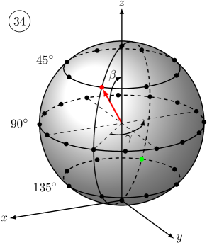
Figure 22: Example of a set of orientation points (black dots) used in direct orientation averaging. The cluster is first rotated by $\gamma$ about the $z$-axis (laser polarization) and then by $\beta$ about the $y$-axis of the laboratory frame.

The weight factors $\lambda_{m}$ are determined by cutting the surface of the unit sphere into segments $\mathcal{S}_{m}$ around unit direction $\mathbf{e}_{m}$ of element $m$. The $\mathcal{S}_{m}$ is defined as the collection of points on the unit sphere which are closer to $\mathbf{e}_{m}$ than to any other $\mathbf{e}_{m^{\prime}}$. The summation weights are then simply the areas of $\mathcal{S}_{m}$ divided by the area of the whole sphere, i.e. $\lambda_{m}=\mbox{Area}(\mathcal{S}_{m})/(4\pi)$.

3.4.2 OAPAD from one-photon processes in the perturbative regime

The direct averaging scheme is conceptually simple and can be applied in any situation. However, it requires a considerable amount of reference orientations (segments) to achieve sufficiently reliable results. A great simplification can be worked out for one-photon processes in the perturbative regime. In that case, one can deduce, using perturbation theory formally, that the rotated PAD can be represented as :

$$\mathcal{A}^{(i)}(\vartheta\phi,\alpha\beta\gamma)=\sum\limits_{\mu\mu^{\prime},lmm^{\prime}}D_{\mu^{\prime}0}^{(1)*}(\alpha\beta\gamma)\,D_{\mu 0}^{(1)}(\alpha\beta\gamma)\,D_{m^{\prime}m}^{(l)}(\alpha\beta\gamma)\,a_{\mu\mu^{\prime},lm^{\prime}}^{(i)}Y_{lm}(\vartheta\phi)\;.$$ (33)

in terms of a couple of expansion coefficients $a_{\mu\mu^{\prime},lm^{\prime}}^{(i)}$, rotation functions $D_{\mu\mu^{\prime}}^{(l)}$ [130], and spherical harmonics. In this form, the integration over Euler angles $(\alpha,\beta,\gamma)$ can be worked out analytically (for details, see [128, 129]), yielding finally the Orientation Averaged PAD as

$$\overline{\frac{{\rm d}\sigma_{i}}{{\rm d}\Omega}}\equiv\overline{\mathcal{A}^{(i)}}(\vartheta\phi) = C_{0}^{(i)}Y_{00}(\vartheta\phi)+C_{2}^{(i)}Y_{20}(\vartheta\phi)\quad,$$ (34)

$$C_{0}^{(i)} = \frac{1}{3}\sum_{\mu}a_{\mu\mu,00}^{(i)}\quad,$$ (35)

$$C_{2}^{(i)} = \sum_{\mu}a_{\mu\mu^{\prime},2\,\mu-\mu^{\prime}}^{(i)}(-1)^{\mu}\times\left(\begin{array}[]{ccc}1&1&2\\ 0&0&0\end{array}\right)\left(\begin{array}[]{ccc}1&1&2\\ -\mu&\mu^{\prime}&\mu\!-\!\mu^{\prime}\end{array}\right)\quad.$$ (40)

The corresponding total PAD is obtained by summing over the s.p. PAD, i.e. $\overline{\mathcal{A}}=\sum_{i}\overline{\mathcal{A}^{(i)}}$. It remains to determine the expansion coefficients $a_{\mu\mu^{\prime},lm^{\prime}}^{(i)}$. Fortunately, there are only very few, that is three for $l=0$ and six for $l=2$. They can be determined from the PAD in only six properly chosen orientations because the different $l$ can be produced from one PAD, see Eqs. (33). The six reference orientations should be chosen such that Eqs. (33) can be solved in a stable manner as a linear equation for the $a_{\mu\mu^{\prime},lm^{\prime}}^{(i)}$. A recommended set is $\mathbf{e}^{(1)}=\mathbf{e}_{x}$, $\mathbf{e}^{(2)}=\mathbf{e}_{y}$, $\mathbf{e}^{(3)}=\mathbf{e}_{z}$, $\mathbf{e}^{(4)}=(\mathbf{e}_{x}\!+\!\mathbf{e}_{y})/\sqrt{2}$, $\mathbf{e}^{(5)}=(\mathbf{e}_{x}\!+\!\mathbf{e}_{z})/\sqrt{2}$, and $\mathbf{e}^{(6)}=(\mathbf{e}_{y}\!+\!\mathbf{e}_{z})/\sqrt{2}$.

The effect of orientation averaging on PAD is demonstrated in Fig. 23.

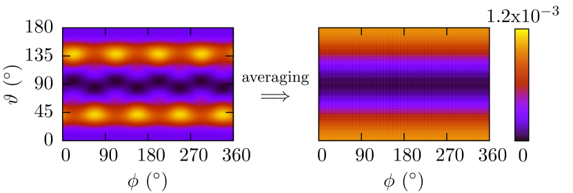
Figure 23: Total PAD $\mathcal{A}(\vartheta,\phi)$ for Na₈ with explicit ionic background for one fixed orientation (left panel) and orientation-averaged (right panel), after laser excitation with frequency $\omega_{\mathrm{las}}=7.5$ eV, intensity $I=10^{11}$W/cm², and pulse length with $T_{\rm pulse}=60$ fs. The emission angles $\vartheta$ and $\phi$ are measured with respect to the laser polarization.

Test case is Na₈ with detailed ionic structure which is, unlike the jellium case, not rotational invariant. The laser frequency is sufficiently high such that one-photon emission dominates. The left panel shows the PAD for a fixed cluster orientation where the cluster symmetry axis is aligned with the laser polarization axis. One sees a pronounced pattern, in particular the four-fold structure of the ionic rings and the rotation of the upper ring by 45^∘ relative to the lower ring. The emission maxima are located at $\vartheta\approx 45^{\circ}$ and $\vartheta\approx 135^{\circ}$, i.e. sidewards to the laser polarization. The orientation averaged PAD becomes independent of $\phi$, as it should be, and the emission is forward/backward dominated with maxima at $\vartheta=0$ and $\vartheta=180^{\circ}$. Altogether, the effect of orientation averaging is dramatic. Calculations for a single orientation have thus little predictive value.

As already pointed out, the OAPAD only depend on the angle $\vartheta$, and not on $\phi$ anymore. Moreover, they are symmetric with respect to the transformation $\vartheta\leftrightarrow-\vartheta$. Thus they can be expanded in a standard manner in terms of even Legendre polynomials $P_{l}(\cos\vartheta)$ as

$$\overline{\frac{{\rm d}\sigma}{{\rm d}\Omega}}\propto 1+\beta_{2}P_{2}(\cos\vartheta)+\beta_{4}P_{4}(\cos\vartheta)+\beta_{6}P_{6}(\cos\vartheta)+...$$ (41)

Most important is $\beta_{2}$, called the anisotropy parameter. It is the only remaining parameter in the perturbative regime where all $\beta_{>2}=0$. Note that we had already recognized the simple $1+\beta_{2}P_{2}(\cos\vartheta)$ structure in Fig. 18.

3.5 Thermal effects

The previous discussions were led assuming that electrons remain at zero temperature. Introducing an ionic temperature in the formalism raises no difficulty as the ions are treated classically. An ionic temperature can thus either naturally build up in the course of time, or be initially introduced by giving the proper velocities to ions. The system, of course, remains globally microcanonical, and the temperature is thus subject to the corresponding fluctuations. The electronic temperature, in turn, is explicitly set to zero by construction. TDLDA does not allow occupation numbers of KS orbitals to vary in time, which prevents an account of thermal effects at the side of the electrons. This is certainly a major formal limitation of the formalism. We have seen that (possibly sizable) electronic temperatures have been observed experimentally (see for example Figure 10). These effects may play a significant role in the understanding of the dynamics of the system, and on the analysis of experimental results. A theoretical account of such thermal effects is thus to be developed.

A standard path to accommodate thermal effects in dynamical systems is to recur to kinetic theory. This theory was originally formulated in the framework of classical mechanics with the Boltzmann equation as a prototypical example [131]. Quantum systems add two more complications. The Pauli principle prevents collisions into occupied states. The uncertainty principle, in turn, raises difficulties when trying to treat collisions locally (as done in the Boltzmann equation). Fully quantal kinetic equations are nevertheless conceivable but much more involved than the classical ones [132, 133] and very hard to apply in finite quantum systems with their discrete spectra. In practice, there is thus no practical quantum theory of such collisional correlations available yet. In turn, semi-classical approaches were developed over the years and allow to cover some situations. The basics is then a version of the Boltzman equation, adapted to account for Pauli principle and known as the Boltzmann-Uehling-Ulhenbeck or Vlasov-Uehling-Ulhenbeck (VUU) equation. It was formally introduced in the early 1930’s [134], then widely used in nuclear dynamics [58, 135], and explored more recently in simple metal clusters [136, 137, 60]. By construction, the VUU equation is semi-classical, which means that details of quantum shell effects are washed out. It is thus applicable, at best, only in highly dissipative situations where the latter shell effects do indeed disappear, or in homogeneous fermionic systems such as electrons in solids [138] or nucleons in a neutron star [139]. In finite fermion systems like clusters and molecules, they are thus bound to high excitation energies, which certainly strongly limits their range of application.

Another point is worth being mentioned here. In realistic calculations, and in spite of the semi-classical treatment, one wants to recover an acceptable description of ground state properties of the studied systems. Experience shows that in electronic systems, this is practically viable only in metal clusters such as sodium clusters [137, 60]. This again strongly restricts the range of applicability of such methods. In particular, it does not allow to attack such widely studied systems as C₆₀ in a fully realistic manner. Still, results obtained in simple metals are interesting and demonstrate the importance of this inclusion of collisional correlations. We will thus briefly present VUU and discuss some of these results here.

There are various ways of introducing VUU but in the case of finite fermionic systems, the simplest and probably best founded presentation is to recur to a semi-classical approximation on top of TDLDA. To perform such a semi-classical limit, we first recast the time-dependent KS (TDKS) equations in a matrix form, by introducing the one-body density matrix ${\hat{\rho}}_{\mathrm{KS}}$ associated to KS states, which reads in real space representation :

$${\hat{\rho}}_{\mathrm{KS}}({\bf r},{\bf r}^{\prime})=\sum_{i=1}^{N}\varphi_{i}^{*}({\bf r}^{\prime})\,\varphi_{i}({\bf r})\quad.$$ (42)

This one-body density matrix fulfills the TDKS equations which, in a matrix form, read :

$$\mathrm{i}\frac{\partial{\hat{\rho}}_{\mathrm{KS}}}{\partial t}=[{\hat{h}}_{\mathrm{KS}},{\hat{\rho}}_{\mathrm{KS}}]\quad,$$ (43)

with $\hat{h}_{\mathrm{KS}}$ given by Eq. (15b). The semi-classical limit can then be attained by performing a Wigner transform (or, even better, an Husimi transform [140]) of Eqs. (42) and (43). This leads to the introduction of the phase space distribution $f({\bf r},{\bf p},t)$ which then fulfills, at lowest order in $\hbar$, the Vlasov equation :

$$\frac{\partial f}{\partial t}=\{h_{\mathrm{KS}}({\bf r},{\bf p},t),f({\bf r},{\bf p},t)\}\quad,$$ (44)

where we have introduced Poisson brackets. At the LDA level, for which the xc functional is local in density, and for simple metals, for which the pseudopotential is local as well, the semi-classical KS hamiltonian takes the following simple form :

$${h}_{\mathrm{KS}}({\bf r},{\bf p},t)=\frac{{\bf p}^{2}}{2m}+U_{\mathrm{KS}}[\rho]+V_{\mathrm{coupl}}({\bf r})+U_{\mathrm{ext}}({\bf r},t)\quad,$$ (45)

where the local density is now obtained from momentum space integration of $f({\bf r},{\bf p},t)$:

$$\rho({\bf r})=\int\frac{\textrm{d}{\bf p}}{(2\pi\hbar)^{3}}f({\bf r},{\bf p},t)\quad.$$ (46)

The Vlasov(-LDA) equation can now be complemented by the effect of ”two-body” collisions as usually done in kinetic theory. This leads to the Vlasov-Uehling-Ulhenbeck (VUU) equation :

$$\frac{\partial f}{\partial t}=\{h_{\mathrm{KS}}({\bf r},{\bf p},t),f({\bf r},{\bf p},t)\}+I_{\mathrm{UU}}[{\bf r},{\bf p}]\quad,$$ (47)

obtained as the Vlasov-LDA equation complemented by a UU collision term :

$$I_{\mathrm{UU}}[{\bf r},{\bf p}]=\int\textrm{d}\Omega\,\textrm{d}{\bf p}_{1}\frac{|{\bf p}-{\bf p}_{1}|}{m}\frac{\textrm{d}\sigma}{\textrm{d}\Omega}\left[f_{\bf p^{\prime}}f_{\bf p^{\prime}_{1}}(1-{\tilde{f}}_{\bf p})(1-{\tilde{f}}_{\bf p_{1}})-f_{\bf p}f_{\bf p_{1}}(1-{\tilde{f}}_{\bf p^{\prime}})(1-{\tilde{f}}_{\bf p^{\prime}_{1}})\right]\;.$$ (48)

which exhibits a local gain-loss balance for elastic electron scattering $({\bf p},{\bf p}_{1})\leftrightarrow({\bf p}^{\prime},{\bf p}^{\prime}_{1})$. The associated cross-section for electron-electron ”two-body” collisions is $\textrm{d}\sigma/\textrm{d}\Omega$ and depends on the relative momentum $|{\bf p}-{\bf p}_{1}|$ and possibly on the scattering angle. We have furthermore used the shorthand notations ${\tilde{f}}_{\bf p}=2\pi\hbar^{3}f_{\bf p}/2$ and $f_{\bf p}=f({\bf r},{\bf p},t)$, the collision term being local in space and time. To avoid a double counting with the mean field $h_{\mathrm{KS}}$ the differential cross-section can be evaluated with a screened Coulomb interaction following standard scattering theory [136, 137, 60, 141].

The Vlasov and VUU equations are best solved using test particle methods rather than grid methods. Practically, this amounts to represent the phase space distribution $f({\bf r},{\bf p},t)$ by a swarm of numerical classical particles $\{({\bf r}_{i},{\bf p}_{i}),i=1,...\}$, each one with a given weight $\omega$ and following classical equations of motion with forces derived from the mean field hamiltonian $h_{\mathrm{KS}}({\bf r},{\bf p},t)$ [142]. Finally, the coupling to classical ionic motion, similarly as in quantal TDLDA, is performed, leading altogether to a Vlasov/VUU-LDA-MD approach. The theory was introduced in cluster physics in the late 1990’s [136] and further used since then [60], but, as already mentioned, only applied to simple metal clusters.

The analysis of Vlasov or VUU dynamics proceeds in a rather simple manner as the elementary degrees of freedom are classical test particles. The total ionization is directly given by the number of test particles ($\times\omega$) outside a large given box in which the Coulomb field is computed. It is equivalently obtained as the integral of the semi-classical density Eq. (46) over this computational box. The latter density also enters the expression of the dipole moment (see Eq. (49) in the next section) to provide an analysis of optical response. The distribution of kinetic energies and the angular distribution are directly extracted from the velocities of the ”emitted” test particles. Note that the semi-classical nature of the approach makes the PES always exponentially decreasing, whatever the excitation, at variance with the quantum case which exhibits the electronic single particles energies. The quantum/classical comparison is then meaningful only at sufficiently large excitations for which the quantum PES is also exponentially decreasing with no more shell structure. The PAD, in turn, can be compared in a meaningful way whatever the excitation energy. For a detailed discussion, see Sec. 4.5.2.

4 Illustrative results

The coordinate-space and real-time technique to solve TDDFT as presented in Sec. 3 offers a powerful tool to describe a broad range of scenarios for the dynamics of clusters and molecules. We present in this section a few illustrative examples of such theoretical studies thereby concentrating on electron ionization and related observables. As a starter, Fig. 24 shows a calculated combined PES/PAD (left column) for C₆₀, compared with an experimental one (right column).

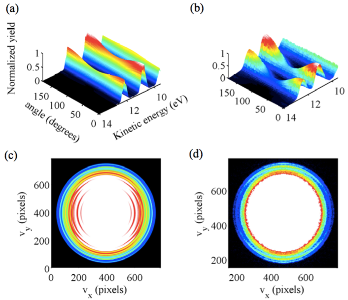
Figure 24: Top : Combined PES/PAD of C₆₀ obtained at $\omega_{\rm las}=20$ eV given by (a) TDLDA-ADSIC calculations ($I=7.8\times 10^{9}$ W/cm² and duration of 60 fs, C₆₀ radius of 6.44 a₀) and (b) experimental measurements using synchrotron radiation with duration of about 1 ps. Bottom : the corresponding velocity map image of (a) is presented in panel (c), and that of (b) in panel (d).

The experimental spectrum was recorded at the Maxlab Synchrotron facility, using an oven to produce the C₆₀ molecular beam [143]. Experiments and calculations are both performed at a photon energy of 20 eV. The top panels present the angle- and energy-resolved distributions of photoelectrons for three selected energies close to the HOMO level in a way similar to Fig. 18, while the bottom panels show the distribution in a polar representation called velocity map images (VMI), see introductory discussion in Sec. 2.3.2 and Fig. 7. The upper panel shows nice agreement between experimental and theoretical results. The VMI in the lower panels also nicely agree for larger energies near the IP (outer part of the circle). But they differ in the low-energy region because it is filled with electrons from thermal emission not accounted for in TDDFT, see also Fig. 36 later on. However, although the physical content of such VMI is very rich, one cannot easily read off a quantitative comparison from such a figure. Therefore, we will in the following sections preferably discuss integrated VMI : PES obtained by integrating over the angle, PAD obtained by integrating over the kinetic energy, and total ionization obtained by integrating over both, energy and angle.

As already mentioned in our first example in Sec. 3.3 and Fig. 18, the peaks observed in a PES are fingerprints of the single particle (s.p.) energies of the electrons before they had been ejected by the photon. However, s.p. energies are usually not well described by LDA. It has to be complemented by a self-interaction correction (SIC) to attain realistic ionization potentials (IP) and thus ionization properties (see Sec. 3.2). Before presenting detailed results on PAD and PES, we first illustrate in Sec. 4.1.1 the capabilities of SIC to properly describe ionization dynamics. We remind again that we describe the processes fully dynamically (see the methodology of Sec. 3.3.5). This means, e.g., that discussing PES does not amount to a mere comparison of a computed static s.p. spectrum with a measured PES. Since our access to PES, PAD, and ionization is fully dynamical, it is thus applicable to any dynamical regime and free of any adjustable parameter. This is why having a proper IP is a crucial step in our dynamical description, especially at low energy where ionization occurs mostly close to threshold, whence the importance of a SIC. Even when dealing with appropriate IP, a word of caution is to be added concerning the interpretation of PES as map of s.p. spectra. There are cases where one finds slight deviations for deep lying s.p. states. These can be understood as correction from final state interaction [144]. They should be considered for a high precision analysis of data. We will ignore the effect in the more principle considerations of this section.

This section is thus organized as follows. In Sec. 4.1, we will first demonstrate the impact of SIC on structural properties as single-electron energies and optical response. In Sec. 4.2, we will discuss ionization as a signal from laser-induced dynamics. Then, in Sec. 4.3, we will address PES, and in Sec. 4.4 PAD, both in the one-photon and in the multi-photon regime. We finally discuss the impact of temperature, either ionic or electronic, on PES and PAD in Sec. 4.5.

4.1 Impact of the self-interaction correction on electronic emission

As just mentioned, ionization properties are very sensitive to the s.p. energies, whence the importance of SIC. We will here demonstrate the impact of SIC on electronic properties, such as s.p. spectrum or optical response, and finally discuss a typical example of PES.

4.1.1 Ionization potentials and single electron spectra

Before starting a discussion of the ionization potential (IP), we have to specify that in more detail. For a system with $N$ electrons, the IP is defined by the difference $I_{\mathrm{adia}}=E(N-1)-E(N)$. This is, in fact, called the “adiabatic IP” if the final values of $E(N-1)$ is taken after waiting for full ionic rearrangement. However, this adiabatic IP is a rather involved observable as it mixes electronic and ionic properties. Much easier to handle and to interpret is the “vertical IP” $I_{\Delta}=E_{\mathrm{fix}}(N-1)-E(N)$ which is obtained from the energy $E_{\mathrm{fix}}$ of the ionized system while still maintaining the ions in their original configuration. This vertical IP is a purely electronic observable which renders it very instructive. In practice, induced ionization processes (laser pulse, ion collision) are so fast that the ionic configuration is almost inert during the emission process. This motivates the use of the vertical IP, henceforth called simply “the IP”.

As already discussed in Sec. 3.2, correct s.p. energies are strongly related to the correct asymptotic behavior of the KS potential, see the example of ${{\rm K}_{7}}^{-}$ in Fig. 16. And as just explained above, the IP is defined as difference of two stationary energies. However, this definition is not well suited to dynamical calculations where one aims at tracking ionization ”on the fly”. For then, it becomes crucial to fulfill Koopmans’ theorem [145] which states that the vertical IP should be identical with the s.p. energy of the last bound electron (HOMO level), i.e. $I_{\varepsilon}=-\varepsilon_{\mathrm{HOMO}}$. Koopmans’ theorem is violated in LDA and usually recovered when invoking SIC. This rules out LDA for a fully dynamical approach to ionization and calls for some SIC. It is thus crucial to test the performance of TDDFT in this respect. As discussed in section 3.2, we have basically a full SIC (practically implemented via the 2setSIC scheme and simply denoted in the following by SIC) and ADSIC at our disposal. ADSIC is orders of magnitude simpler than SIC and thus certainly worth being considered very seriously. As a first step, we shall thus check the capabilities of both approaches with respect to reproducing IP’s along the lines of a large systematic study in [108].

Fig. 25 depicts the difference between the calculated IP and the experimental one, for a selection of molecules.

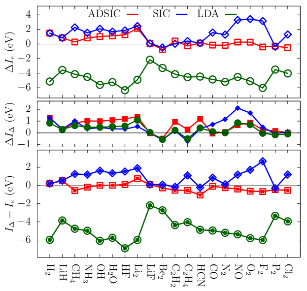
Figure 25: Calculated ionization potentials (IP) of a selection of molecules with different bonding types for various level of SIC (see text for details). Top : difference $\Delta I_{\varepsilon}=I_{\varepsilon}-I_{\mathrm{exp}}$ of the IP $I_{\varepsilon}$ deduced from the energy of the HOMO with the experimental (vertical) IP $I_{\mathrm{exp}}$. Middle : difference $\Delta I_{\Delta}=I_{\Delta}-I_{\mathrm{exp}}$ for the IP $I_{\Delta}$ calculated as the difference of binding energies. Lower : non-Koopmans’ error $I_{\Delta}-I_{\varepsilon}$. Adapted from [108].

Both ways are used for the calculations : from the HOMO level as $-\varepsilon_{\mathrm{HOMO}}$ (upper panel, open symbols) or from the difference of binding energies $I_{\Delta}$ (middle panel and filled symbols). The upper panel shows that, as expected, LDA performs badly when one considers the IP $I_{\epsilon}$ from the energy of the HOMO. SIC and even more so ADSIC come much closer to the experimental IP. The middle panel compares the IP $I_{\Delta}$ from energy differences. Here we see better agreement for all three methods, demonstrating that the $I_{\Delta}$ is the more robust definition. To emphasize the discrepancy between both estimates of IP’s, we plot their difference in the lower panel of Fig. 25. Vanishing difference signifies fulfillment of Koopmans’ theorem. LDA produces large errors while SIC and ADSIC do well. It is a bit of a surprise that the simpler ADSIC often performs better than the more elaborate SIC.

By construction, ADSIC is a priori well suited to systems with metallic binding [106]. It was nevertheless soon realized that it also performs well in covalent systems [107]. The very systematic study of [108] led to the unexpected result that for an enormous range of atoms, molecules, carbon chains, and fullerenes ADSIC leads very often to smaller non-Koopmans errors than SIC. It was also shown that, when comparing theoretical IP’s to experimental ones, again ADSIC was providing the best results for a huge range of molecules. That however does not mean that ADSIC is the ultimate solution to the self-interaction problem. We have already mentioned its intrinsic limitations (essentially due to the fact that the functional explicitly depends on the number of electrons) in Sec. 3.2 and we should add here that the scaling properties of ADSIC with increasing system size are also raising some problems [108]. Furthermore, there are a few specific cases which raise difficulties. These are molecules where very different types of bonding coexist, such as covalent and metallic bonding. The point is illustrated in Fig. 26 which presents the s.p. energies of the two complexes NaH₂O and Na(H₂O)₂, calculated in LDA, ADSIC and SIC. The right part of the figure complements the picture by showing the corresponding non-Koopmans errors.

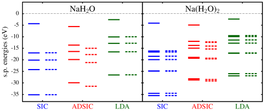
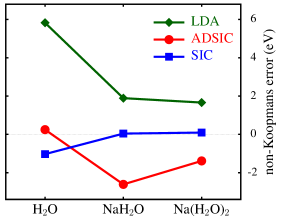
Figure 26: Single particle energies of NaH₂O (left) and Na(H₂O)₂ (middle) in LDA, ADSIC and SIC, for spins up (full lines) and down (dashes). Right : non-Koopmans’ error calculated in various levels of DFT as indicated. From [146].

Not surprisingly the water molecule with one prevailing bonding type is well described in ADSIC, while SIC yields a small but somewhat larger non-Koopmans’ error. The situation becomes different in the mixed complexes Na(H₂O)_n, where both ADSIC and LDA exhibit similarly large errors (although with opposite signs), while the Koopmans’ theorem is perfectly fulfilled in SIC. Thus ADSIC should not be used for Na(H₂O)_n. This may not be a total surprise if one reminds that ADSIC applies the same correction to every orbital while, in such a mix of bonding types, one encounters both highly delocalized metallic orbitals and much more localized covalent orbitals. As visible in the left panel of Fig. 26, the HOMO in NaH₂O at 5.14 eV arises from the Na atom whereas the deeper orbitals mostly come from the H₂O molecule, which has an IP of 12.6 eV (see Fig. 1). The electronic density of the HOMO is thus clearly different from that of the other orbitals, so that self-interaction for different electronic states becomes very different.

The example of a metal-covalent complex shows that ADSIC is not a safe fire solution to the self-interaction problem. It is likely to fail whenever the s.p. states cover grossly different regions of space. This also occurs in the fragmentation of a molecule and in processes with high ionization. Nonetheless, ADSIC provides very often a remarkably accurate and simple approximation to SIC. It is always worthchecking whether a given problem allows one to employ ADSIC. In the following examples, we will often recur to ADSIC.

4.1.2 Optical response

One of the most prominent observables of electronic dynamics is the optical response measured in terms of the photo-absorption strength. It gives insight into the spectrum of dipole transitions and provides useful information on the collective modes and the particle-hole excitations of the system. Note that the word ”optical” is generic in the sense that it covers also the spectrum outside the optical range of frequencies. Consider, for instance, covalent systems where the dominant peaks rather lie in the UV domain. Here, we want to explore the impact of SIC on the optical response.

The optical response can be calculated in various ways. It is often evaluated by computing the response function directly in linearized TDLDA. Having a fully fledged TDLDA code at hand, it is technically and conceptually simpler to employ spectral analysis for that purpose [86, 147, 148]. To that end, we initialize the electronic dynamics by applying an instantaneous dipole boost to the electronic wave functions. We then record the time-dependent dipole momentum :

$$\mathcal{D}(t)=\int\textrm{d}^{3}\mathbf{r}\,(\mathbf{r}-\mathbf{R}_{\mathrm{cm,ion}})\,\rho(\mathbf{r},t)\quad,$$ (49)

where $\mathbf{R}_{\mathrm{cm,ion}}$ denotes the center of mass of the ions. The dipole strength $S_{D}(\omega)$ is obtained by Fourier transforming $\mathcal{D}(t)\longrightarrow\tilde{\mathcal{D}}(\omega)$ yielding finally $S_{D}(\omega)\propto\Im\{\tilde{\mathcal{D}}(\omega)\}$. One can alternatively look at the power spectrum $|\tilde{\mathcal{D}}(\omega)|^{2}$ which basically contains the same information as the dipole strength.

We already presented in the bottom right part of Fig. 1 the optical response calculated in ADSIC of H₂O in the three spatial directions. Fig. 27 now displays the power strength averaged over the three spatial directions, and compares the calculations done in LDA with those in ADSIC.

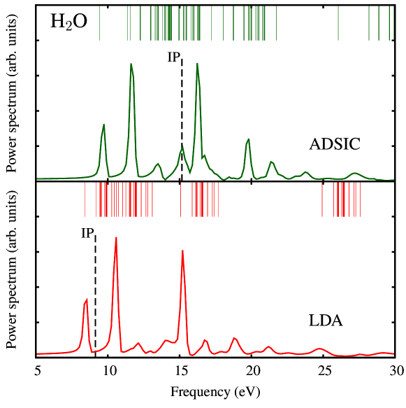
Figure 27: Optical response of H₂O calculated in LDA (bottom) and ADSIC (top). The dashes indicate the ionization potential (IP) calculated as the opposite of the HOMO energy. The vertical full lines stand for the possible static dipole transitions.

Each photo-absorption spectrum is complemented by the sequence of one-particle-one-hole ($1ph$) states with dipole character calculated from the static s.p. energies of occupied and empty states. First, we notice that the distribution of $1ph$ states in LDA is very different to that in ADSIC. This reflects the different s.p. spectra of LDA and ADSIC. ADSIC tends to localize the wave functions more than LDA which results in a more compact electron cloud (associated to a larger IP) and a wider span of dipole transitions. It is also interesting to note that most LDA dipole transitions lie in the continuum (IP$\simeq 9.1$ eV). In spite of these large differences in $1ph$ spectra, the dipole spectra look very similar. The reason is that the recoupling of the pure $1ph$ states to the true excited states is dominated by the Coulomb Hartree term [149, 150] which is the same in LDA and SIC. This defines the overall position of dominant dipole strength which is more or less robust. The underlying $1ph$ structure has an impact on the detailed fragmentation pattern which can depend more sensitively on the level of SIC treatment. The payoff between Coulomb interaction and $1ph$ structure depends, of course, on the system. Metal clusters have the pronounced Mie plasmon mode which is dominated by the Coulomb interaction, thus very robust against SIC. On the other hand, systems with fuzzy dipole spectra are more critical. The example H₂O is somehow in between.

4.1.3 SIC-revisited photoelectron spectra

Since the early days of DFT, the interpretation of Kohn-Sham (KS) orbitals has been a matter of debate. A direct comparison of experimental PES spectra to s.p. spectra or even better so to our dynamically computed PES (see Sec. 3.3.5) is an a posteriori proof of the meaning to be given to KS s.p. energies, following the basic multiphoton ionization (MPI) relation (9). The point is rather easy to accept at the LDA or ADSIC level to the extent that the KS hamiltonian ${\hat{h}}_{\rm KS}$ (see Eq.(15b)) is well defined and common to all KS orbitals. The situation is more involved in the case of SIC where the KS hamiltonian (18) becomes state-dependent. The ”2setSIC” solution scheme (18–21) allows, nonetheless, to define unambiguously s.p. energies. It is thus interesting to see how SIC performs for computing PES, to see to which extent the SIC s.p. energies have a similar meaning as in LDA or ADSIC. Rather than making a comparison to experiment, which will not test the internal capabilities of the theory, it is here more interesting to check the evolution of the PES peaks within varying the laser frequency and see whether they follow the MPI rule (9). This would give an indication on their possible interpretation. The point is illustrated for the case of the planar metal cluster Na₅. Two different laser pulses have been used with frequencies 8.16 and 10.9 eV. The laser intensities have been adjusted in each case to obtain about the same low total ionization around 0.006, thus well in the perturbative regime where PES signals are not yet blurred by Coulomb shift (see Secs. 4.3.4 and 4.3.5.2). The laser polarization is taken normal to the cluster’s plane. Fig. 28 displays both PES.

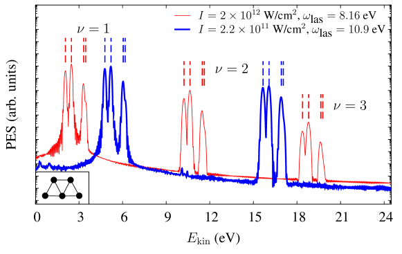
Figure 28: Photoelectron spectra for Na₅ (ionic configuration in the inset) irradiated by two different laser pulses with pulse duration of 60 fs, intensity $I$ and frequency $\omega_{\mathrm{las}}$ as indicated, and polarized along the direction normal to the Na₅ plane. The static Kohn-Sham orbital energies, shifted by $n\omega_{\mathrm{las}}$ where $\nu$ is the number of involved photons, see Eq. (9), are also indicated as vertical dashed lines in both cases. Adapted from [151].

For a given laser frequency $\omega_{\mathrm{las}}$, one clearly observes copies of the same pattern which are separated by $\omega_{\mathrm{las}}$. Each pattern exhibits peaks which are positioned at values of the kinetic energy $E_{\mathrm{kin}}$ following the standard MPI relation Eq.(9), i.e. $\varepsilon_{\mathrm{kin},j}=\varepsilon_{j}+\nu\,\hbar\omega_{\mathrm{las}}$. The $\varepsilon_{j}$ entering this equation are the eigenvalues of the stationary equation $h_{\mathrm{SIC}}|\varphi_{j}\rangle=\varepsilon_{j}|\varphi_{j}\rangle$, see Eq. (21), while $\nu$ corresponds to the number of photons involved. The remarkable fact that the peaks of the PES, obtained from the calculation of a time propagation of the 2 sets $\{\varphi_{j}\}$ and $\{\psi_{\alpha}\}$, coincide with the static $\varepsilon_{j}$ validates the interpretation (and the definition) of these energies as sound s.p. energies. This also supports the identification of the $\varphi_{j}$’s as the physical wave functions of the associated s.p. states whose characteristics are measurable via the PES.

4.2 Using ionization as an observable

In this section, we discuss basic mechanisms in the laser irradiation of an electronic system leading to significant electronic emission and their analysis in terms of total ionization as an observable. For moderate laser intensities, a major issue is the relation of the laser frequency with the optical response peaks, especially collective ones. We will present here two generic scenarios for this resonance effect. We will first explore laser irradiation of a water molecule demonstrating off- and on-resonant ionization. In Sec. 4.2.2, we will take advantage of resonant enhancement of ionization to explore the ionic dynamics via the use of a pump-and-probe (P&P) setup. In Sec. 4.2.3, we will finally consider again a P&P setup, but this time within using a train of attosecond pulses.

4.2.1 Off- and on-resonant ionization

As already discussed in Sec. 1.2, the great versatility of lasers through the choice of frequency, intensity, pulse duration and shape, offers experimentalists and theoreticians a world of dynamical scenarios. To gather orientation in this huge landscape of options, we first explore the impact of laser frequency. To that end, we consider the dynamics of laser excitation of a H₂O molecule, with techniques similar to those used in [152]. The results are shown in Fig. 29.

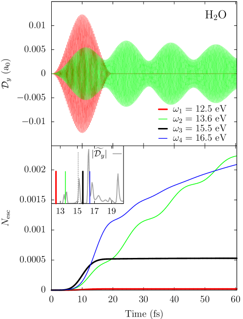
Figure 29: Resonant and off-resonant irradiation of H₂O by laser pulses polarized along the symmetry axis of H₂O, denoted by $y$, and of various intensities ($I_{1}=10^{12}$, $I_{2}=I_{3}=10^{11}$, $I_{4}=10^{9}$ W/cm²) and various frequencies ($\omega_{1}=12.5$, $\omega_{2}=13.6$, $\omega_{3}=15.5$, $\omega_{4}=16.5$ eV). Calculations had been done with ADSIC and pseudopotentials to leave core electrons inert. Top : time evolution of the electronic dipole in $y$ direction. Bottom : time evolution of the total ionization $N_{\mathrm{esc}}$. Inset : optical strength of H₂O in $y$ direction with horizontal energy axis in eV. The vertical full lines indicate the chosen laser frequencies, and the dotted one corresponds to the IP, here at 15.1 eV.

The duration of the laser pulses is in all cases 20 fs. Four frequencies have been explored, namely $\omega_{1}=12.5$, $\omega_{2}=13.6$, $\omega_{3}=15.5$ and $\omega_{4}=16.5$ eV. The corresponding intensities are $I_{1}=10^{12}$, $I_{2}=I_{3}=10^{11}$ and $I_{4}=10^{9}$ W/cm² to keep the maximal dipole amplitude similar. The laser polarization is along the symmetry axis of the water molecule, denoted here by $y$.

Let us start with $\omega_{1}$ and $\omega_{2}$. Both frequencies are below the IP of H₂O (15.1 eV). The optical response of H₂O in $y$ direction is shown in the inset in the bottom panel : $\omega_{2}$ lies on a double peak and, as we will see, corresponds to a resonant frequency, whereas $\omega_{1}$ does not match any dipole transition and is thus off-resonant. The top panel of Fig. 29 shows the time evolution of the electronic dipoles. As expected [14], the red curve for the off-resonant $\omega_{\mathrm{las}}=\omega_{1}$ nicely follows the laser pulse profile and dies out with the laser signal at 20 fs. The total ionization $N_{\mathrm{esc}}$ shown in the bottom panel (red line) stays very close to zero for this low frequency case. The resonant $\omega_{\rm las}=\omega_{2}$ proceeds differently : During the first 15 fs, the dipole signal (light green curve in top panel) still follows the laser profile, but then continues to oscillate with large amplitude long after the laser pulse is switched off. Such resonant oscillations come along with a larger deposit of energy in the molecule and thus stronger ionization. This is clearly demonstrated in the bottom panel of Fig. 29, where $N_{\mathrm{esc}}$ (green line) steadily increases with visible steps perfectly correlated to the maxima in the dipole oscillations. The total ionization $N_{\mathrm{esc}}$ in the resonant case is orders of magnitude larger than in the off-resonant one, although the laser intensity in the resonant case is 10 times smaller. This can be understood in terms of the Keldysh parameter (8) which is, in both cases, much larger than 1. This indicates that we are in the frequency-dominated regime where such differences matter, see Sec. 1.2.2.

Note also the initial profile of the ionization is determined by the laser pulse such that the maximum slope coincides with the laser peak amplitude. But this profile is delayed by the time it takes for the escaping electrons to reach the box bounds. The final non-vanishing slope is related to the non-vanishing dipole oscillations.

The next two cases consider an off-resonant frequency ($\omega_{3}$) and a resonant one ($\omega_{4}$), now both above the IP. For the sake of clarity, the corresponding dipole signals are not displayed. They show again the same typical pattern of resonant (long standing after-oscillations) and off-resonant (signal dies out with the laser) response. We only show the associated total ionization $N_{\mathrm{esc}}$ in the bottom panel of Fig. 29 (black thick line for $\omega_{3}$ and blue thin line for $\omega_{4}$). The off-resonant case increases with a slope following the amplitude of the dipole oscillations and levels off to a plateau after the laser pulse is over. The case $\omega_{3}$ yields much higher ionization than the case $\omega_{1}$, even if its intensity $I_{3}$ is an order of magnitude smaller than $I_{1}$. This happens because $\omega_{3}$ stays above the IP and can ionize directly with one-photon processes. Finally we compare the two resonant cases $\omega_{2}<$IP with $\omega_{4}>$IP. Although $I_{2}/I_{4}=100$, both $N_{\rm esc}$ are very similar. Two effects cooperate here : i) $\omega_{4}>$IP and ii) the strength of the mode excited at $\omega_{4}$ is at least 3 times stronger than that at $\omega_{2}$. This demonstrates, once again, the importance of the laser frequency in relation to the optical spectrum in order to drive large ionization.

The point is again illustrated, this time in a more systematic manner, in Fig. 30 which displays the dependence on laser frequency of the total ionization $N_{\mathrm{esc}}$ of irradiated C₆₀ (left) and ${{\rm Na}_{41}}^{+}$ (right).

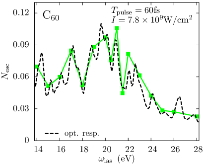
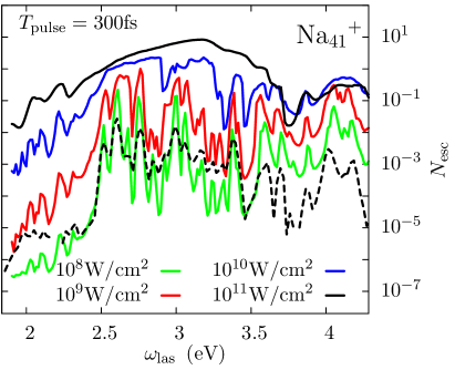
Figure 30: Total ionization $N_{\mathrm{esc}}$ as a function of laser frequency $\omega_{\rm las}$. Left : case of C₆₀, calculated in full 3D with a radius of 6.44 a₀, irradiated by a laser pulse with $T_{\mathrm{pulse}}=60$ fs and $I=7.8\times 10^{9}$ W/cm². Right : case of ${{\rm Na}_{41}}^{+}$ irradiated by laser pulses with $T_{\mathrm{pulse}}=300$ fs and intensities $I$ as indicated (using CAPS). The black dashed line represents the optical response in both cases.

The figure is a continuation to the pedagogical Fig. 4 discussed in Sec. 2.1, this time for two more complex systems though. For C₆₀, with the chosen laser parameters ($I=7.8\times 10^{9}$ W/cm² and $\omega_{\mathrm{las}}=$14–28 eV), we are again in the frequency-dominated regime. The ionization $N_{\mathrm{esc}}(\omega_{\mathrm{las}})$ (light green curve) exhibits strong oscillations with $\omega_{\mathrm{las}}$ which match remarkably well the optical response of C₆₀ (black dashed line). This shows that the signal of photoemission $N_{\mathrm{esc}}(\omega_{\mathrm{las}})$ is close to the signal of photo-absorption, at least above the emission threshold.

The situation is similar in ${\mathrm{Na}_{41}}^{+}$ at the lowest laser intensity (light green curve in right panel) where $N_{\mathrm{esc}}$ exhibits strong oscillations with $\omega_{\mathrm{las}}$, once again fitting fairly well those of the optical spectrum. However, if the laser intensity is increased, we progressively leave the frequency-dominated regime to enter the field- (intensity-)dominated domain (see Sec. 1.2.2). And indeed, the fragmented structure of $N_{\rm esc}$ steadily broadens to be finally washed out at the highest intensity (see top black curve). At the same time, the values of $N_{\mathrm{esc}}$ for a given $\omega_{\mathrm{las}}$ also increase, since there are more and more photons pulling on the valence electrons of the cluster.

4.2.2 Pump and probe (P&P) analysis of ionic dynamics

The emergence of fs lasers allowed the development of time-resolved studies of molecular reactions through pump-and-probe (P&P) experiments. The typical strategy of such a fs spectroscopy is simple. An initial short laser pulse (pump) excites the electronic system which leads to subsequent ionic motion. This motion in turn changes the electronic response according to the actual ionic configuration. This change is explored by the response (e.g., ionization) of the system to a second laser pulse, the probe, sent after a certain time delay. Scanning the reaction strength as a function of delay time allows one to map the time evolution of the molecular system. There are, of course, many variants of this generic strategy according to the variety of molecules and flexibility of laser pulses. Altogether, fs spectroscopy has become an extremely powerful analyzing tool in physics and chemistry, for early reviews, see [153, 154].

Of course, P&P analysis is also an extremely interesting tool in cluster physics. Very small clusters allow scenarios very similar to those in simple molecules, see e.g. experiments on trimers [155, 156] and associated theory [157]. Larger clusters are too complex for the very subtle and detailed pathways followed in small molecules. One better looks for global properties of the ionic background as, e.g., radius or deformation, and one needs prominent signal in the dense electronic spectrum. Metal clusters are distinguished by the dominant Mie surface plasmon resonance [9], whose peak frequency is predominantly determined by cluster radius and deformation. Thus there are many P&P studies on metal clusters, either free, deposited on a surface, or embedded in a substrate, see e.g. Sec. 5.3.4 of [12].

As P&P experiments on clusters are rather demanding, early studies achieved a comparable, although coarser, effect by varying the temporal width of a single laser pulse. For an early example on Pt clusters, see [33]. We exemplify this type of analysis here for the case of Ag clusters embedded in a He droplet for better handling [158].

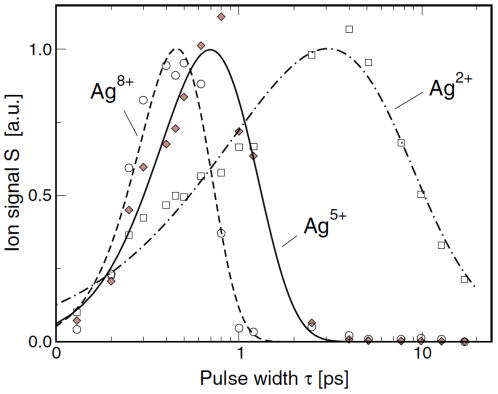
Figure 31: Yields for selected Ag^q+ ions after irradiation of a Ag cluster with a laser pulse of wavelength 800 nm, drawn as a function of the width $\tau$ of the the laser pulse. For the shortest pulse of 130 fs, the peak intensity is $I_{0}=1.2\times 10^{14}$ W/cm². For other $\tau$, the fluence $\propto\tau\,I_{0}$ has been kept constant. The data are normalized for better comparison, and the fit curves serve as a guide to the eye. From [158].

The clusters are irradiated with laser pulses of fluence $\tau\,I_{0}=156$ W fs/cm² (where $\tau$ is the pulse width and $I_{0}$ the peak intensity). This strong pulse leads to a disintegration of clusters producing all sorts of fragments and highly ionized Ag atoms. The charge state $q$ of the emerging Ag^q+ ions is an indicator for the violence of the reaction and thus for the strength of the laser-cluster coupling. Fig. 31 shows the ion yield as a function of pulse width. All ionization stages $q$ show a strong dependence on $\tau$ with a distinct maximum for a certain $\tau$. This optimum pulse width, which was already observed in [33], results from an interplay of (ongoing) laser pulse, ionic expansion, and plasmon frequency. The IR laser pulse first triggers ionization. The Coulomb pressure thus generated leads to a slow expansion of the cluster. And the plasmon frequency (originally in the visible range) decreases with increasing radius, until the laser comes into resonance with the plasmon with subsequently strong energy absorption and violent reaction. If the laser pulse is too short, it is over before resonant conditions are reached. If it is too long, it becomes too weak (remind the constant fluence thus implying decreasing intensity with increasing pulse duration) to trigger sufficient expansion. Such a maximum is seen in Fig. 31 for each charge state, however at different delay times $\tau$. The interpretation given in [158], furthermore, addresses a subtle point in laser experiments. The laser intensity is not constant over the spatial width of the beam. It decreases when going away from the focus. Thus clusters outside the focus receive a weaker signal than those right in the focus of the beam. It is assumed that these lower charge states are related to lower intensities out of focus. Therefore, the experiment so to say produces at once results for different laser fluences.

The rather involved P&P analysis is easier for clusters in/on a substrate because this allows a higher density of reactive centers. Therefore, most P&P studies on clusters are performed in/on substrate. The typical setup is that of a chromophore in an inert substrate. The latter thus serves mainly as a support for the cluster. The principles and the richness of P&P analysis remain unaffected by the inert substrate. There is a couple of measurements of an electronic property, the electronic relaxation time, for clusters on surfaces in a variety of material combinations [159, 160, 161]. More typical for P&P analysis is the study of ionic oscillations which has been performed, e.g., for Ag clusters embedded in glass matrix [162, 163]. A much more gentle support is provided by liquid He clusters, which were already used as useful laboratory for studying molecular properties under well controlled conditions [164]. The He environment couples such softly to any other material that one can consider the embedded system as being practically free. There are then several instructive P&P experiments of Ag clusters in He droplets, e.g. [38, 165] (called “dual pulse” experiments in these publications). A detailed description of the large scale dynamics of Ag clusters is very expensive. Theoretical investigations are thus often performed for Na clusters as practicable model systems for metal clusters [166, 167, 165].

The dominance of the Mie plasmon peak in metal clusters allows a particular P&P strategy which does not rely on directly hitting the resonance but uses just the distance of the Mie plasmon frequency to the laser frequency to map the underlying ionic dynamics. This strategy has been studied in detail for the global breathing (radius oscillations) of Na clusters in [166] and for the dynamics of cluster deformation in [167]. We illustrate the scheme here for the case of breathing. Fig. 32 shows the result of a theoretical exploration for the cluster ${{\rm Na}_{41}}^{+}$ using TDLDA for electronic dynamics coupled to molecular dynamics for the ionic motion [168, 14, 12].

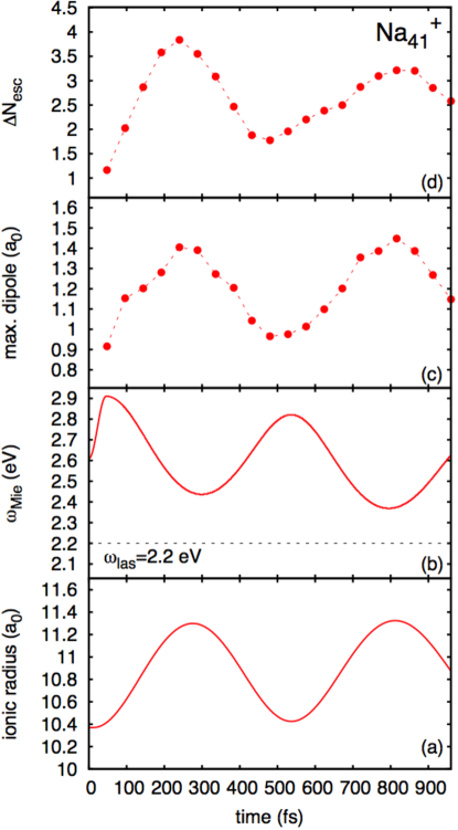
Figure 32: Pump and probe spectroscopy of ionic breathing vibrations of ${\mathrm{Na}_{41}}^{+}$ using the Mie plasmon resonance as indicator. Panel (a): time evolution of the ionic r.m.s. radius, $\sqrt{\sum_{I}{\bf R}_{I}^{2}}$, after the pump pulse. Panel (b): time evolution of the Mie plasmon frequency after the pump pulse. The laser frequency $\omega_{\mathrm{las}}=2.2\,\mathrm{eV}$ is indicated as horizontal dashed line for comparison. Panel (c): maximum amplitude of the dipole response to the probe pulse as a function of time delay. Panel (d): additional ionization $\Delta N_{\mathrm{esc}}$ induced by the probe pulses as a function of time delay. Pump and probe pulses have the same properties: photon frequency $\omega_{\rm las}=2.2\,\mathrm{eV}$, intensity $I=1.1\!\times\!10^{12}$ $\,\mathrm{W/cm}^{2}$, and a sin² shape with FWHM$=24\,\mathrm{fs}$. The pump laser produces very quickly an initial emission of $N_{\mathrm{esc}}=3$ electrons, thus delivering a total charge state $q=4^{+}$. After [166].

The cluster ${{\rm Na}_{41}}^{+}$ is nearly spherical. The pump pulse ionizes it quickly to charge state ${{\rm Na}_{41}}^{4+}$. This produces a Coulomb pressure which triggers slow breathing oscillations of the whole cluster, while deformation is negligible along the whole dynamics. The radius oscillations after the mere pump pulse are shown in panel (a) of the figure. The Mie plasmon resonance depends on charge state and cluster radius. An estimate is shown in panel (b). One sees the fast initial blue-shift due to the fast initial ionization to $q=4^{+}$. After that, one finds oscillations which perfectly follow the radius oscillations according to $\omega(t)\propto R(t)^{-3/2}$ [150]. The laser frequency for the probe pulse is also indicated. It was chosen safely below the Mie resonance such that the actual Mie frequencies never cross. The electronic response to the probe pulse is small if the Mie frequency is far from the laser, and large if it comes close. This can be seen in panel (c) from the maximum amplitude of the dipole signal during the probe pulse. The strong dipole response leads to further ionization shown as additional number of escaped electrons $\Delta N_{\mathrm{esc}}$ in panel (d). It is, of course strongly correlated with the dipole amplitude. Tracing the chain of correlations back to panel (d), we can conclude that the extra ionization directly maps the global ionic radius using the scheme with the remote laser frequency as an “observer”. Net ionization thus provides a direct (time resolved) analysis of ionic motion, in that case dominated, on the rather short times considered, by radial oscillations. The actual long term evolution of the system is, in fact, Coulomb explosion. The interesting aspect is that the long path to explosion is accompanied by monopole (radial) oscillations which are directly visible in the ionization signal (actually via the plasmon peak).

Almost all P&P studies on clusters have used the ionization yield as an observable. One expects that one could learn more from more detailed observables, particularly from time-resolved PES and PAD. Such experiments are, of course, much more complex and still more demanding than the, already intricate, traditional P&P measurements. Nonetheless, first studies in that direction have been published [169, 170] so far in the regime of hefty excitations. The field is widely open for further studies in more moderate excitation regimes.

All the P&P studies, including the above example, show that the ionization yield can depend sensitively on the choice of the laser pulse characteristics. As the temporal profile and all other laser parameters can be tuned in an extremely flexible manner, the question naturally arises whether one could tune laser pulses for maximum yield (or other desired reaction properties). This is the idea of ”optimal control” which is of particular importance in chemistry and molecular physics, see e.g. [171, 172]. Again, the application to large clusters is more involved and allows more strategies to be tracked. An interesting study using optimal control, e.g., to trigger the yield of highly charged Ag atoms from Ag clusters can, nevertheless, be found in [173].

While addressing promising future developments of P&P studies, we ought to mention the upcoming availability of attosecond pulses. These allow P&P studies which resolve features of electronic dynamics. We will discuss that in the next section 4.2.3.

4.2.3 Towards P&P experiments with attosecond pulses

Electron dynamics can also be analyzed at its own pace if one is able to handle pulses much shorter than typical electronic time scales in the fs regime. This is nowadays experimentally accessible down to some hundreds of attoseconds, at least in the form of a train of attosecond pulses. This yields access to details of electronic dynamics subject to electromagnetic perturbations. Early convincing tests were performed in simple atoms such as He and Ar [174] on the basis of a P&P setup involving a UV atto-train on top of an IR field. It was shown that the total ionization may exhibit marked oscillations as a function of the delay between UV train and IR signals, once the repetition rate of seven attopulses per train is chosen to be half the IR period. The analysis of these experiments was supported by simple simulations using the Time-Dependent Schrödinger Equation (TDSE) with a single active electron. The TDSE also served as a basis for further theoretical investigations, either directly [175, 176, 177] or in perturbation theory [178]. These approaches gave convincing clues on the origin of the modulation of the ionization but so far, no robust many-electron theory is available to explain the observations.

More recently, experiments were generalized to simple molecules with qualitatively similar results as in the atomic case, although with a slightly different combination of IR and UV pulses [179, 180, 181]. The first fully microscopic calculations were performed on this occasion and led to results remarkably compatible with experiments [182]. The actual interpretation of the underlying mechanism is nevertheless, again, to be understood in more detail. Still, the remarkable agreement between theory and experiments is worth being presented and discussed in one test case.

We consider here the N₂ molecule as a test case [182]. The laser pulse consists in an IR component :

$$V_{\rm IR}(t)=E_{\rm IR}f_{\Delta T}(t)\sin(\omega_{\rm IR}t)\quad,$$ (50)

with a frequency $\omega_{\rm IR}=1.58$ eV and with a sin² pulse profile $f_{\Delta T}$ of FWHM$=\Delta T/2\simeq 29$ fs (see Eq.(2)). At the same time is superimposed a train of $n$ attopulses, each of them labeled by $i$, which reads :

$$V_{\rm atto}(t) = \sum_{i=1}^{n}E_{\rm atto}(\tilde{t})\,f_{\delta t}(\tilde{t}-t_{i})\sin\left[\omega_{\rm UV}(\tilde{t}-t_{i})\right]\,e^{-4\tilde{t}^{2}/\Delta T^{2}}\;,$$ (51a)

$$t_{i} = \Delta t+(i-1)[\delta t+\delta t^{\prime}]\;,$$ (51b)

$$\tilde{t} = t-\Delta t\;,$$ (51c)

where $\delta t\simeq 0.29$ fs is the actual duration of each individual attopulse, and $\delta t^{\prime}$ the time separation between two successive attopulses. The attopulse train (APT) is delayed by a variable delay $\Delta t$ with respect to the IR pulse (starting at t=0). Both the IR pulse and the APT are linearly polarized. The individual attopulse shape is again a sin² profile (see Eq. (2)) of FWHM$=\delta t/2$. A key point of the setup is to fix the time interval between two successive attosecond signals. We choose here $\delta t+\delta t^{\prime}=T_{IR}/2\simeq 1.30fs$, which is exactly half the IR period. The amplitude of the APT is further modulated by a Gaussian envelop of width such that the total APT duration is about half (29 fs) the total duration of the IR pulse. This fixes the number $n$ of attopulses which is, in this case, 22. The peak intensity of the IR pulse is chosen to be $I_{\rm IR}=10^{12}$ W/cm², while that of the attopulses is, at maximum of the Gaussian envelope, $I_{\rm atto,0}=10^{10}$ W/cm². Finally, the frequency of the APT lies in the UV domain, $\omega_{\rm UV}=20.4$ eV, so that each individual attopulse contains about 1.5 UV oscillation. The laser parameters are such that the pure IR pulse does not lead to ionization, while a pure UV train does lead to some ionization through one-photon processes because the IP of N₂ is around 16.3 eV $<\omega_{\rm UV}$. The remarkable result of the experiments is that combining the IR and the attopulses leads to a significant enhancement of ionization (while it only adds 1.58 eV on top of the UV photons already above the continuum). Moreover, this enhanced ionization is strongly modulated by the delay $\Delta t$. Ionization actually exhibits marked oscillations as a function of delay with a period equal to half the IR period. Maxima of oscillations are attained for delays such that the attopulses are in phase with maxima or minima of the IR pulse, which explains the doubled frequency of ionization maxima as compared to the IR frequency.

The case is illustrated in Fig. 33 where we have plotted the total ionization, the average kinetic energy of emitted electrons and the anisotropy $\beta_{2}$ characterizing the PAD (see Eq. (41) and Sec. 4.4).

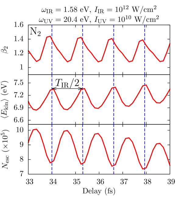
Figure 33: N₂ ionization properties irradiated by an IR pump and an attopulse train (see text for details) as a function of delay time between attopulse train and IR pulse. Bottom : total ionization. Middle : average kinetic energy per emitted electron, see Eq. (52). Top : anisotropy parameter $\beta_{2}$, see Eq. (41). The faint dashed lines indicate the sequence of maxima and minima regularly separated by half the IR period. Adapted from [182].

As one UV photon suffices for ionization, $\beta_{2}$ provides a complete characterization of the PAD. The average kinetic energy is defined as

$$\langle E_{\rm kin}\rangle=\frac{\hbar^{2}}{2m}\int\textrm{d}\mathbf{r}\,\frac{{\bf j}^{2}({\bf r})}{\rho({\bf r})}\,\left[1-{\cal M}^{2}({\bf r})\right]\quad,$$ (52)

where $m$ is the electron mass, ${\bf j}({\bf r})$ is the local current, $\rho({\bf r})$ the local density and ${\cal M}({\bf r})$ the mask function used to evaluate emitted electrons (see Eq. (23f)). It provides a simple measure of the PES in terms of one number. All three signals in Fig. 33 display remarkable oscillations as a function of delay time $\Delta t$ with a period equal to half the IR period. Both $\langle E_{\rm kin}\rangle$ and $\beta_{2}$ oscillate in phase and in opposite phase with the total ionization respectively. Indeed, if the deposited energy content is about the same, the higher the ionization, the lower their average kinetic energy. And not surprisingly, the more energetic the emitted electrons, the more aligned the emission along the laser polarization axis and the larger the $\beta_{2}$. These oscillations of the total ionization perfectly match those observed experimentally. A comparison with PES and PAD has to wait until these quantities are experimentally available.

We finally end this discussion by mentioning recent experimental P&P dynamics which use XUV pulses for both the pump and the probe. This is at variance with the example discussed above, where the pump is an IR pulse and the XUV probe is constructed from some of its high order harmonics using the so-called RABITT (Reconstruction of Attosecond Beating by Interference of Two-photon Transitions) technique [183, 184]. To distinguish the two kinds of P&P, one sometimes quotes them as IR-pump-XUV-probe and XUV-pump-XUV-probe experiments respectively. One type of setup uses a coherent splitting of a XUV light produced by a FEL. For instance, this technique has been successfully applied to small molecules as N₂ and O₂ [185], or C₂H₂ [186]. In these latter examples, the XUV frequency is 38 eV, the photon intensity between $10^{11}$ and $10^{13}$ W/cm², and the XUV pulse duration of 30 fs. The delay time resolution is 1 fs, and the whole delay time can vary over the $\pm 350$ fs range. The advantage of using XUV light for the pump and the probe is to ionize the species under study by absorption of a few photons, at variance with an IR pulse. Therefore, this P&P setup can follow the induced Coulomb explosion at a time scale of a few fs. Very recently, some experiments went even further by taking advantage of high harmonic generation from an IR pulse irradiating an atomic gas jet : the produced XUV attopulses are then separated from the IR pulse, filtered to keep only one pulse which is at the end split into two coherent XUV as pulses. This brand new technology has been applied in the irradiation of Xe atoms [187] and the H₂ dimer [188]. The XUV intensities are about $10^{13-14}$ W/cm², their duration about 600 as, their frequency is 14 eV, and the delay time is well below 1 fs. Such an experimental apparatus thus enables to track the Coulomb explosion dynamics over the whole reaction path and on a time scale never attained before. In both XUV-XUV P&P experiments, fragment or ion yields are measured as a function of delay time. To the best of our knowledge, no electronic observable has been measured so far. There are also very few real-time calculations of such a dynamics [188, 189]. They employ a time-dependent Schrödinger equation of the full electronic and nuclear wave function (note however that only vibronic modes – no rotational mode – are considered in these calculations). For light atoms as those in H₂, a quantal description of the nuclei is probably compulsory. The necessity of such a fully quantal treatment is more questionable for heavier atoms, as in N₂. Anyway, the computational cost of such calculations becoming too prohibitive for larger covalent systems, this probably calls for a classical treatment of the ions, even if H⁺ nuclei come into play.

4.3 Dynamical aspects in photoelectron spectra

We have discussed above how (static) s.p. spectra can be extracted from the peaks observed in PES using Eq. (9), see for instance Fig. 28. This identification can be worked out by perturbation theory and requires a laser with moderate intensity and high frequency resolution. True dynamical processes exploit more of the versatility of lasers. The aim of this section is thus to discuss the impact of the laser parameters frequency, intensity, and pulse duration on PES, and find out how dynamical aspects can be analyzed through PES.

4.3.1 Impact of pulse duration

Any laser pulse of finite duration delivers a distribution of frequencies about its mean frequency $\omega_{\mathrm{las}}$. The longer the pulse, the sharper this distribution. One can evaluate the width of this distribution by calculating $\sigma_{\mathrm{las}}=\int_{0}^{\infty}(\omega-\omega_{\mathrm{las}})^{2}\,|\tilde{I}(\omega)|\,\textrm{d}\omega$ where $\tilde{I}(\omega)$ is the Fourier transform of the time-dependent laser intensity $I(t)$. As an illustration, we give in the following table some widths related to pulse duration at $\omega_{\mathrm{las}}=20$ eV[190].

$T_{\mathrm{pulse}}$ (fs)	10	30	60	75	200	1000
$\sigma_{\mathrm{las}}$ (eV)	0.44	0.16	0.083	0.068	0.027	0.0058

Table 1: Width of frequency distribution for different laser pulse durations, around a mean value of $\omega_{\mathrm{las}}=20$ eV.

One consequence of the finite frequency width of the laser pulse is that a PES (in the perturbative regime) does not display a sharp spike exactly at $E_{\mathrm{kin}}=\varepsilon_{i}+n\omega_{\mathrm{las}}$, but a more or less soft peak around this $E_{\mathrm{kin}}$. Finite pulse duration thus produces a broadening of the PES peaks, the larger the shorter the pulse. To exemplify this effect, Fig. 34 displays PES of Na₂ irradiated by laser pulses of intensity $10^{11}$ W/cm², frequency $\omega_{\mathrm{las}}=6.8$ eV, and a couple of different pulse durations from 50 to 400 fs.

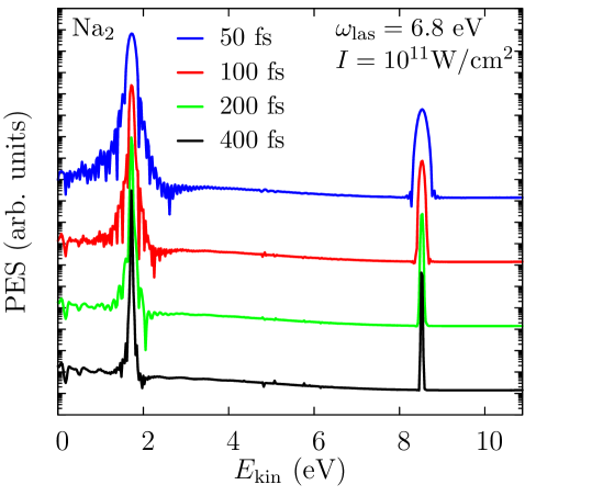
Figure 34: Photoelectron spectra of Na₂ after irradiation by laser pulses of indicated characteristics. Some PES have been up-shifted for the sake of clarity.

We clearly observe an increasing resolution of the PES peaks with increasing pulse duration. This holds as long as the intensity of the laser pulse remains sufficiently low. Higher intensities can blur this picture because ongoing ionization induces a drift of the peaks due to a Coulomb shift of the levels. This will be addressed in Secs. 4.3.4 and 4.3.5.2.

4.3.2 Impact of laser polarization

In section 2.3.2, we have seen that a combined PES/PAD, that is an energy- and angle-resolved photoelectron spectrum, can deliver a lot of information on the dynamics of the photoemission. In the perturbative regime, it reveals the angular distribution for emission from specific s.p. states. A simplified view can be obtained by restricting the analysis to two specific directions : one parallel to the laser polarization axis ($\theta=0,180^{\circ}$) and one perpendicular to it ($\theta=90^{\circ},270^{\circ}$). The point is illustrated in Fig. 35 where calculated parallel and perpendicular PES of ${{\rm Na}_{7}}^{-}$ are plotted.

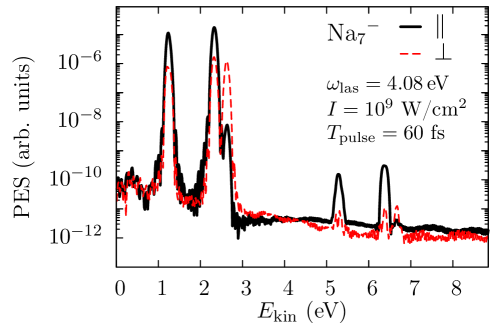
Figure 35: Photoelectron spectra of ${\mathrm{Na}_{7}}^{-}$ for a given orientation, irradiated by a laser with parameters as indicated. Black full curve: PES along the laser polarization axis. Red dashes: PES in the direction perpendicular to it. Calculations were done in cylindrical approximation for the electronic potentials.

The sodium cluster has a fixed orientation here (orientation averaging will be discussed in Sec. 4.4). The calculated s.p. energies are $\varepsilon_{1}=-2.82$ eV, $\varepsilon_{2}=-1.72$ eV, and a pair of almost degenerate $\varepsilon_{3,4}=-1.43$ eV. As in the case of Na₅ (see Fig. 28), the peaks of the PES perfectly fulfill the relation $E_{\mathrm{kin}}=\varepsilon_{i}+\nu\omega_{\mathrm{las}}$ with $\nu=1,2$. The first group of peaks between 1 and 3 eV corresponds to $\nu=1$. States 1 and 2 predominantly emit along the laser polarization axis, while states 3 and 4 show a clear preference of emission in perpendicular direction. The 2-photon process (between 5 and 7 eV) suppresses even more strongly the perpendicular direction, and thus the parallel photoemission dominates. This indicates a general feature of multiphoton emission : the higher the photon number $\nu$, the larger the anisotropy $\beta_{2}$ corresponding to an increasing dominance of emission parallel to the laser polarization axis.

4.3.3 Impact of laser frequency

The estimate (9), i.e. $E_{\mathrm{kin}}=\varepsilon_{i}+\nu\omega_{\mathrm{las}}$, of PES peaks establishes correctly the relation between peaks at $E_{\mathrm{kin}}$ and corresponding s.p. energies $\varepsilon_{i}$. However, it does not tell anything about the strength with which the peaks appear. And here, we can have dramatic differences between one-photon processes and multiphoton ones. As an illustration, we show in Fig. 36 ionization pattern of C₆₀ in the one-photon (left panels) and in the multi-photon (right panels) regimes [191].

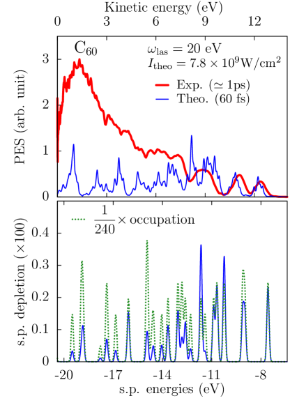
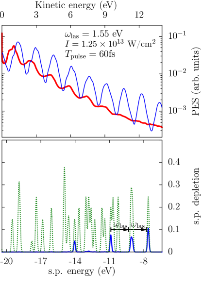
Figure 36: Top : Theoretical and experimental photoelectron spectra of C₆₀ with radius of 6.763 a₀ and orientation averaging. Bottom : Calculated single particle depletion (blue full lines) compared with static occupation numbers (green dots). Left : one-photon regime ($\omega_{\mathrm{las}}=20$ eV), laser pulse length of 60 fs and intensity of $7.8\times 10^{9}$ W/cm² (theory) or a synchrotron irradiation of duration of about 1 ps. Right : multi-photon regime with $\omega_{\mathrm{las}}=1.55$ eV, laser pulse length of 60 fs and intensity of $1.25\times 10^{13}$ W/cm², both in theory and experiment. In the bottom left panel, the single particle depletions are multiplied by 100 for a better comparison. Adapted from [191].

Orientation averaging presented in Sec. 3.4 has been applied in the theoretical calculations, to allow a comparison with experimental measurements. The upper panels compare theoretical and experimental PES, and the lower panels show as complementing information the depletion (blue full lines) and the occupancy (green dotted lines) of the corresponding s.p. levels. The one-photon case was already presented in Fig. 24 which compares theoretical and experimental combined PES/PAD and VMI. The laser pulse in this case experimentally stems from synchrotron radiation at 20 eV with a pulse duration of about 1 ps. Theoretical calculations were done for the same frequency, intensity $I=7.8\times 10^{9}$ W/cm², but shorter pulse $T_{\mathrm{pulse}}=60$ fs for practical reasons. In the one-photon regime ($\omega_{\mathrm{las}}\gg$ IP), we do not expect that the pulse duration is essential. Calculations yield a total ionization of about 0.006. In the multi-photon case, the theoretical parameters are chosen as in the experiment, that is $T_{\mathrm{pulse}}=60$ fs, $I=7.8\times 10^{9}$ W/cm², and $\omega_{\mathrm{las}}=1.55$ eV. Here, the calculated total ionization is about 0.07. Comparing both cases (one- and multi-photon), PES and depletion pattern are completely different. The one-photon case also shows a marked difference between experiment and theory. This has to be discussed in detail.

The bottom panels of Fig. 36 display the s.p. levels (with occupation weight) and their depletion. For $\omega_{\mathrm{las}}=20$ eV (lower left panel), all states can emit by a one-photon process. And indeed, we observe that most states contribute to the total ionization. As expected, the theoretical PES resembles the s.p. depletion pattern very much [192].

We now turn to the multi-photon case (right panels of Fig. 36). With the laser frequency chosen here, at least 6 photons are needed to bring electrons from the HOMO into the continuum. Since the probability of ejection decreases with the number of photons required, only the least bound states can be significantly depleted. And this is what is observed in the right bottom panel : the states which emit the most are the HOMO, HOMO$-1$ and HOMO$-3$, precisely separated by about $\omega_{\mathrm{las}}=1.55$ eV. Therefore, we cannot expect that the PES maps the whole s.p. energy spectrum. Indeed, the theoretical PES exhibits oscillations consisting in a broad peak repeated several times, separated by $\omega_{\mathrm{las}}$ from one copy to the other. These oscillations constitute the typical multiphoton ionization (MPI) pattern (see Sec. 2.1). Each one of these MPI peaks is rather well bundled due to the fact that the few emitting states line up rather well with the photon frequency.

In both cases (one- and multi-photon), the experimental PES differ from the theoretical ones. The difference looks particularly large for the one-photon case (upper left panel). Here, the PES are still fairly comparable at higher energies (7–13 eV). While theoretical calculations were done at the ground state configuration (zero temperature), the experimental peaks are broadened due to ionic vibrations of C₆₀ which are rather large at the experimental temperature of 900 K. A huge discrepancy between theory and experiment is observed at low electron kinetic energy. The experimental PES grows almost an order of magnitude above the theoretical one. We think that these low-energy electrons stem from electron-electron collisions which hinder part of the electrons from being directly emitted, but rather lead to auto-ionization mechanisms or thermal electron emission. Such dynamical electron-electron correlations are not included in TDLDA. So we are missing here most of the low-energy electrons. This could be cured with theories beyond TDLDA which will be discussed in Sec. 4.5.2. For the time being, the comparison between experiment and theory is relevant only for the highest photoelectron energies dominated by direct electron emission. And there, the agreement is very satisfying.

A difference between experimental and theoretical PES is also seen in the multi-photon regime (upper right panel). We first note a shift between the position of the theoretical peaks and that of the experimental ones. This might be due to a slight uncertainty in the determination of the experimental intensity and/or pulse duration, which can then produce a different ionization stage. And we will see that this can cause a sizeable (Coulomb) redshift, see Secs. 4.3.4 and 4.3.5.2 below. Moreover, the amplitude of oscillations of PES decreases with increasing kinetic energy in the measurements, while it remains more or less constant in the theoretical calculations. Once again, the dynamical correlations, which are missing in the theory, are most probably the mechanism responsible for the damping of the oscillations in the experimental data.

4.3.4 Impact of laser intensity

A couple of experimental PES had already been shown in Fig. 10 for the case of C₆₀ irradiated by laser pulses of various intensities. The results seemed to be all in the same regime marked by smooth, exponentially decreasing PES throughout. Another example was just given above in Fig. 36 where the top right panel shows typical MPI pattern of repeated peaks which have at least an exponentially decreasing envelope. For a more systematic survey, we now discuss computed PES for two different clusters. As a first example, we discuss a set of PES of ${{\rm Na}_{41}}^{+}$ (see left panel of Fig. 37) obtained with the same laser frequency (3.8 eV) and pulse duration (300 fs) but with varying intensities (from bottom to top) starting from $I_{0}=10^{9}$ W/cm² and up to $300\,I_{0}$.

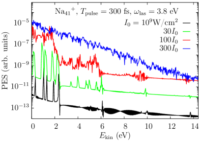
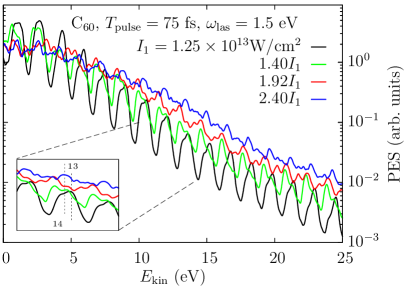
Figure 37: Calculated photoelectron spectra for various intensities. Left : case of ${{\rm Na}_{41}}^{+}$ irradiated by laser pulses of duration of 300 fs, frequency of 3.8 eV, and $I_{0}=10^{9}$ W/cm² (calculations done with CAPS). Right : case of C₆₀ (calculated in full 3D with radius of 6.44 a₀ and with orientation averaging) irradiated by laser pulses of duration of 75 fs, frequency of 1.5 eV, and $I_{1}=1.25\times 10^{13}$ W/cm². The inset zooms in the 10–14 eV range with the 13-photon ionization of the HOMO and the 14-photon one of the HOMO$-1$.

The chosen frequency of 3.8 eV is basically off-resonant, as the dominant plasmon response of ${{\rm Na}_{41}}^{+}$ lies in the spectral range between 2.5 and 3.1 eV. Since the IP of ${{\rm Na}_{41}}^{+}$ is 5.3 eV, the first peaks at low kinetic energies in Fig. 37 stem from two-photon processes. The pulse duration is 300 fs to allow a high spectral resolution of the PES peaks, as is observed in the lowest PES (black curve). The laser intensity is also small enough to stay in the perturbative regime, since the total ionization $N_{\mathrm{esc}}$ is 0.004 in this case. When the laser intensity is increased by a factor 30 (light green curve), one can spot a slight broadening of the peaks, although the PES still shows clear signatures of the underlying s.p. spectrum. The broadening develops to the side of lower kinetic energies, in total yielding a weak red-shift of the peaks. It is to be noted that the total ionization amounts to $N_{\mathrm{esc}}=0.1$ now. This ionization enhances the Coulomb binding in the course of the electron emission which, in turn, leads to a down-shift of the s.p. energies, called henceforth “Coulomb shift” [119] : electrons which are emitted later in the process see a deeper binding and thus escape with lower kinetic energy. A time-resolved PES would allow one to observe more clearly how the Coulomb shift builds in the course of time. This will be discussed in more detail in Sec. 4.3.5.2 and Fig. 39. Note also the appearance of multi-photon peaks with this larger intensity. Two-photon processes grow $\propto I^{2}$ and so the absorption of more photons becomes more probable.

At the next stage, $I=100\,I_{0}$, the PES is already smeared to broad steps. Here, $N_{\mathrm{esc}}=0.54$ and the Coulomb shift significantly blurs the PES. But still, we can distinguish blocks of one-, two-, and three-photon processes. Finally, the highest intensity of $I=300\,I_{0}$ produces an ionization of $N_{\mathrm{esc}}=4.1$ and the PES are fully smoothed to an exponential decrease with almost no structure left, resembling a “thermal” PES. But an exponential PES alone is not a sufficient indicator of thermalization. More information contained in PAD can help in that respect, as was briefly mentioned in Sec. 2.3.2. We will address this point in detail in Secs. 4.4 and particularly 4.5.2.

We finally discuss the case of PES in a highly multi-photon regime, shown in the right panel of Fig. 37. The studied system is here C₆₀ and the laser has a pulse duration of 75 fs and a frequency of 1.5 eV. Five laser intensities $I$ have been considered : $I_{0}=1.25\times 10^{13}$ W/cm², $1.2\,I_{0}$, $1.4\,I_{0}$, $1.92\,I_{0}$, and $2.4\,I_{0}$. The total ionization of course increases with $I$ : $N_{\mathrm{esc}}=0.03$, 0.06, 0.12, 0.31, and 0.60. With the chosen frequency, we need at least 6 photons to extract electrons (the IP is here 8 eV). At the lowest intensities, we clearly observe the typical MPI patterns of repeated copies of the peak. The peaks are gradually red-shifted when we increase the laser intensity which is, again, the Coulomb shift. Moreover, the red-shift increases with laser intensity due to increasing ionization and finally washes out all structures at the highest $I$. The disappearance of the MPI peaks is illustrated in the inset zooming into the 13-photon ionization of the HOMO and the 14-photon ionization of the HOMO$-1$. The net conclusions from that case are the same as those from ${{\rm Na}_{41}}^{+}$. But here, it becomes even more obvious that the envelope of MPI follows in any regime an exponential decrease. Taking this together with the smoothing due to high ionization delivers then the purely exponential profile resembling thermal emission.

4.3.5 More on the role of plasmon

4.3.5.1 Competition between laser and plasmon frequencies

Thus far, we have discussed PES emerging from the interplay between s.p. energies and the pulse frequency. This simple view has to be modified in the vicinity of strong excitation modes of the system. In particular, the dominant Mie surface plasmon in metal clusters can also have a large impact on the PES. To illustrate this point, we discuss the irradiation of ${{\rm Na}_{9}}^{+}$ by laser pulses with duration of 48 fs, intensity of $10^{9}$ W/cm², and six different laser frequencies $\omega_{\mathrm{las}}$ in the vicinity of the Mie plasmon frequency of ${{\rm Na}_{9}}^{+}$, $\omega_{\mathrm{pl}}=2.7$ eV. The resulting PES are depicted in Fig. 38.

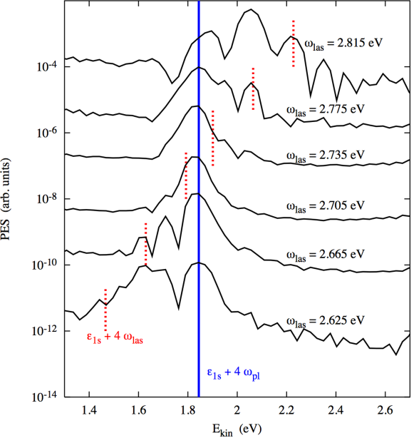
Figure 38: Photoelectron spectra in the energy range of the 4-photon process (red vertical dots at $\varepsilon_{1s}+4\omega_{\mathrm{las}}$) of the $1s$ state of ${\mathrm{Na}_{9}}^{+}$, after irradiation by laser pulses with duration of 48 fs, intensity of $10^{9}$ W/cm², and six different frequencies $\omega_{\mathrm{las}}$ as indicated. The blue solid vertical line indicates the the 4-plasmon process located at $\varepsilon_{1s}+4\omega_{\mathrm{pl}}$, with $\omega_{\mathrm{pl}}=2.7$ eV. Adapted from [193].

The peak of the pure four-photon process, located at $\varepsilon_{1s}+4\omega_{\rm las}$, is indicated for each laser frequency by vertical dots. The position of this peak moves to the blue with increasing $\omega_{\mathrm{las}}$. Additionally, one observes a peak whose position does not depend on the laser frequency, indicated by the solid vertical line. Its position matches the energy of a 4-plasmon process, i.e. $\varepsilon_{1s}+4\omega_{\mathrm{pl}}$. When $\omega_{\mathrm{las}}$ is sufficiently separated from $\omega_{\mathrm{pl}}$ (see the two lowest and the two uppermost curves), one can easily disentangle the four-photon process from the four-plasmon one. The four-plasmon peak actually dominates the PES in most of the cases, a further indication of the already discussed resonant ionization mechanism (see Fig. 29 and 30 in Sec. 4.2.1). In most cases, one can even conceive a coexistence of plasmon and photon excitations. For instance, the uppermost curve shows three prominent peaks, that is the four-plasmon peak, the four-photon peak, and in between a two-plasmon–two-photon peak. For reasons not yet well understood, we cannot find significant signals of a mix of one-plasmon–three-photon or three-plasmon–one-photon processes.

4.3.5.2 Towards time-resolved PES

The above example dealt with the excitation of a resonance mode through a close, although not exactly matching, laser frequency. Resonant modes may also be excited by laser pulse whose frequency $\omega_{\mathrm{las}}$ is far away from the resonance, but where a multiple of $\omega_{\mathrm{las}}$ coincides with the mode. Such a situation should also leave traces in the PES. We exemplify that for the case of Na₈ irradiated by a laser polarized along the symmetry axis of the cluster, denoted by $z$, a pulse duration of 120 fs, a frequency of 1.1 eV and an intensity of $3.1\times 10^{11}$ W/cm². The Na₈ cluster consists in two squares parallel to a plane (denoted by $x$ and $y$) and which are twisted by $45^{\circ}$ around the $z$ axis. It possesses three states of energies $\varepsilon_{1s}=-5.75$ eV, $\varepsilon_{1p_{xy}}=-4.5$ eV and $\varepsilon_{1p_{z}}=-4.2$ eV. The optical response is dominated by the Mie plasmon at 2.5 eV. But there are also further strong peaks in the optical response, especially one located at $\omega_{\rm sat}=3.2$ eV. With $\omega_{\mathrm{las}}=1.1$ eV, the laser pulse is clearly off-resonant. One thus expects a time evolution of the electronic dipole in phase with the laser pulse, as it was the case in the off-resonant irradiation of a water molecule, see Fig. 29. This is indeed the case during almost the whole pulse duration, as is visible in the left panel of Fig. 39.

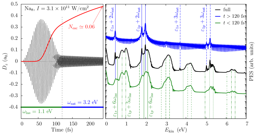
Figure 39: Electronic dynamics of Na₈ after irradiation by a laser with polarization along $z$, duration of 120 fs, frequency of $\omega_{\mathrm{las}}=1.1$ eV and intensity of $3.1\times 10^{11}$ W/cm² (calculations with pseudopotentials and in full 3D). Left : Time evolution of electronic dipole along the symmetry axis of Na₈, denoted by $z$, and of ionization $N_{\mathrm{esc}}$. The horizontal bars emphasize time spans dominated by the indicated frequencies, that is by $\omega_{\mathrm{las}}$ below 90 fs and by a satellite frequency $\omega_{\mathrm{sat}}=3.2$ eV. Right : corresponding PES evaluated in different time windows : during the first 120 fs (green or light curve), after 120 fs (blue or dark curve), and for the full time span (black curve). The various PES have been augmented with scale factors to separate them in the plot. The vertical lines indicate the $1s$, the degenerate $1p_{xy}$ and the $1p_{z}$ energies shifted by multiples of $\omega_{\mathrm{las}}$ (lower lines) or of $\omega_{\mathrm{sat}}$ (upper lines). All single electron energies have been down-shifted by 0.18 eV to account for the Coulomb shift due to the total ionization of 0.06 at the end of the simulation time. Adapted from [194].

A higher frequency however appears from 100 fs on, precisely at $\omega_{\mathrm{sat}}$. It persists even after 120 fs when the laser is switched off, since sizable oscillations remain at this higher frequency. One should moreover notice that $\omega_{\mathrm{sat}}\simeq{3}\,\omega_{\mathrm{las}}$, which indicates that absorption of three photons from the laser pulse triggers this excitation. It is a typical example for higher harmonic generation. The persistence of dipole oscillations provokes a continuous electronic emission. Thus the total ionization $N_{\rm esc}$, also plotted in the left panel of Fig. 39 as a red curve, does not level off after 120 fs but rather increases with a constant slope, reaching the value of 0.06 at the end of the simulation time.

It is interesting to observe how the PES builds up in time in such a case. To this end, we plot in the right panel of the PES calculated for the full time span, and compare it to that calculated for the first 120 fs (green lower curve) and that after 120 fs (blue upper curve). One observes a slight down-shift of the peaks from the early to the late time windows. This provides a time-resolved illustration of the Coulomb shift (discussed in Sec. 4.3.4). Due to the final $N_{\rm esc}=0.06$, an average Coulomb shift of the s.p. energies of $\delta\epsilon=-0.18$ eV emerges. Hence the latter energies, indicated by vertical lines, have been shifted by $\delta\epsilon=-0.18$ eV to achieve a better matching with the PES peaks. The full PES (black middle curve) shows patterns repeated with equal spacing which are, at first glance, MPI peaks, as seen before for C₆₀ (see right panel of Fig. 36). The first peak near zero kinetic energy is related to a four-photon process emitting out of the $1p_{z}$ state. Most of the peaks in this full PES can be identified with $E_{\mathrm{kin}}=\varepsilon_{i}+\nu\omega_{\mathrm{las}}$, as indicated by the bottom vertical lines. There are, however, further peaks not explained in terms of photon frequency. To disentangle the peaks, we have also evaluated the PES in two time windows, an early one during the laser pulse, i.e. 0-120 fs, and a late one after the pulse is over. The PES for the early window (lower green curve) is fully explained by MPI with the laser frequency. The PES from the late window (upper blue curve) shows sharp peaks which can be identified as multi-resonance peaks located at $\varepsilon_{i}+\mu\omega_{\mathrm{sat}}$, with $\mu=2,3$ (we have also applied here the same red-shift $\delta\epsilon$). No MPI peak from the laser shows up in the late window. Note also that the multi-resonance peaks already slightly develop during the laser pulse (see vertical lines from above).

In this example, we have thus demonstrated that a dynamical competition between various frequencies, here that from the laser pulse and that from a higher resonance matching the third harmonics of the laser, can provide mixed mappings of the PES and can thus give rise to a complex structure of the PES. A time-resolved PES analysis can be a way to disentangle the different contributions. To that end, even a coarse time resolution as performed here may be sufficient.

4.4 Photoelectron angular distributions (PAD): a sensitive tool

This section is devoted to PAD. We are using free clusters as examples. Thus we consider orientation averaged PAD throughout, see Sec. 3.4. Remind that these can be expanded in terms of Legendre polynomials $P_{2k}(\cos\theta)$ according to Eq. (41). The expansion parameters $\beta_{2k}$ carry all information about the orientation averaged PAD. The largest non-vanishing $\beta_{2\nu}$ is related to the number $\nu$ of photons involved in the process. The most important parameter is the anisotropy $\beta_{2}$ which is also the only relevant parameter for one-photon processes. Therefore, $\beta_{2}$ will play a key role in the following presentations.

4.4.1 One-photon regime

4.4.1.1 Stationary state picture and Bethe-Cooper-Zare formula

The study of PAD has a long standing history, especially in atoms. Early works by Bethe [195] and Cooper and Zare [196, 197] are still routinely used in today’s cluster literature [17, 198]. The Bethe-Cooper-Zare formula delivers a compact expression for the evaluation of $\beta_{2}$ in spherical potentials. At variance with our standard way of evaluating PAD (see Sec. 3.3.4), it provides a stationary state picture which thus requires evaluation of both bound and continuum electronic states to describe initial and final electronic states. By construction, it does not include possible electronic rearrangement effects following electronic emission, as was demonstrated in [194]. This limits the applicability to cases where electronic rearrangement (through Coulomb residual interaction) can be neglected. Furthermore, being developed for atomic physics, the Bethe-Cooper-Zare is strictly limited to spherical external potentials. Nonetheless, it may be useful as zeroth order estimate and reference.

The Bethe-Cooper-Zare formula was first derived in first-order perturbation theory for one-electron atoms in [195]. But it can also be applied to many-electron systems in an independent-state picture where the many-body wave function is a simple anti-symmetrized product of s.p. orbitals [196, 197]. For a given electronic level $i$, the total cross-section $\sigma^{(i)}$ for emission and its anisotropy $\beta_{2}^{(i)}$ are given by [199, 200]:

$$\sigma^{(i)} =\frac{(4\pi)^{2}\mathcal{N}}{3}\cdot\frac{L\mathcal{R}_{-}^{2}+(L+1)\mathcal{R}_{+}^{2}}{(2L+1)}\>,$$ (53)

$$\beta_{2}^{(i)} =\frac{L(L\!-\!1)\mathcal{R}_{-}^{2}+(L\!+\!1)(L\!+\!2)\mathcal{R}_{+}^{2}-6L(L\!+\!1)\mathcal{R}_{-}\mathcal{R}_{+}\cos\Delta}{(2L+1)[L\mathcal{R}_{-}^{2}+(L+1)\mathcal{R}_{+}^{2}]}\>,$$ (54)

with

$$\mathcal{R}_{\pm} =\int_{0}^{\infty}\textrm{d}r\,r^{3}R_{L\pm 1}^{(f)}(r)R_{L}^{(i)}(r)\quad\text{and}\quad\Delta=\Delta_{L+1}-\Delta_{L-1}\>,$$ (55)

$$\mathcal{N} =\frac{4\pi^{2}e^{2}\omega_{\mathrm{las}}}{\hbar c}\>.$$

where $L$ is the angular momentum of the initial state. Once given the (spherical) potential, the radial wave functions of bound state $R_{L}^{(i)}$ and continuum state $R_{L\pm 1}^{(f)}$ can be calculated by solving the associated radial Schrödinger equation. The phases $\Delta_{L\pm 1}$ entering the continuum states can be obtained in a standard manner from the asymptotic behavior of the outgoing wave $R_{l}^{(f)}$ [201].

Note that in the particular case of a spherical wave function ($L=0$), the Bethe-Cooper-Zare formula exactly delivers $\beta_{2}^{(s)}=2$ (maximum possible value of $\beta_{2}$ in the one-photon domain). In this case, the angular distribution of $s$ states is not influenced by the radial form of the outgoing wave, so that the potential does not affect the angular distribution; it only impacts the cross-section (53).

In spite (or maybe because) of its simple compact form, the Bethe-Cooper-Zare formula has thus to be taken with a grain of caution in realistic cases, because of its strong dependence on the shape of bound and unbound electronic wave functions (see Fig. 40 below). Furthermore, it remains a stationary state picture thus well inside the perturbative regime, when applicable (spherical potential). Its range of application is thus limited.

4.4.1.2 On the sensitivity of $\beta_{2}$ to model assumptions

There are several approximations around in the description of clusters and molecules. The above mentioned Bethe-Cooper-Zare formula for instance forces spherical symmetry and neglects electronic rearrangement. Fully dynamical calculations often employ reduced symmetries as, e.g., in CAPS or by using a jellium model for the ionic background. Many of these approximations are validated for describing spectra and global emission properties. However, PAD is very sensitive to this kind of theoretical details, and one has to check carefully the impact of approximations.

We test the sensitivity for the simplest case of one-photon processes which are fully characterized by the anisotropy $\beta_{2}$. To have a systematic test, we study variations of $\beta_{2}$ as a function of laser frequency. We take as a test case Na₈ and consider $\beta_{2}^{(1p)}(\omega_{\mathrm{las}})$, that is, the anisotropy parameter for emission out of the $1p$ state [202]. To explore the impact of dynamical rearrangement effects in the PAD, the left panel of Fig. 40 compares results of a fully dynamical TDLDA-ADSIC calculation (full blue line) with the result of the Bethe-Cooper-Zare formula or, alternatively, with a TDLDA calculation in which the electrons are propagated in the frozen ground-state Kohn-Sham potential (dashed red line).

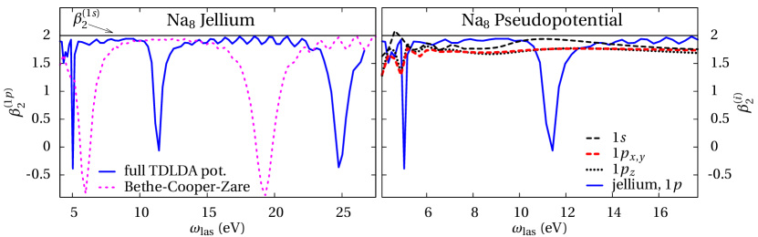
Figure 40: Anisotropy parameters $\beta_{2}^{(i)}$ of single particle states $i$ in Na₈, as a function of laser frequency $\omega_{\mathrm{las}}$. Left : $\beta_{2}$ of the $1p$ shell in Na₈ described by a spherical jellium ionic background (Wigner-Seitz radius $r_{s}=3.65$ a₀, surface thickness $\sigma=1$ a₀), calculated in TDLDA-ADSIC (full blue line), and in a Bethe-Cooper-Zare approach, see Eq. (54) (pink dotted curve). For the $1s$ level, $\beta_{2}^{(1s)}=2$ at any $\omega_{\mathrm{las}}$. Right : $\beta_{2}$ of the $1s$, $1p_{x,y}$, and $1p_{z}$ shells in Na₈ described by explicit ions and pseudopotentials, and averaged over six orientations. For a better comparison, $\beta_{2}^{(1p)}$ from the jellium calculation is superimposed. Adapted from [202].

Note that the result of the Bethe-Cooper-Zare formula is basically identical to a dynamical calculation with the KS potential kept fixed at its static form and driven at very low laser intensity to stay safely in the one-photon regime. The laser pulse duration is of 60 fs and its intensity is scaled with the frequency ($I=10^{13}$ W/cm² $\times\omega_{\mathrm{las}}$) to keep the total ionization in the range between $10^{-4}$ and 0.1, and thus to stay in a perturbative regime. The laser frequency is varied between 4.1 and 29 eV, so that only one photon is needed to promote the electron from the $1p$ state into the continuum ($\varepsilon_{1p}=-4.08$ eV). The ionic background of Na₈ is treated by a spherical jellium (Wigner-Seitz radius $r_{s}=3.65$ a₀, surface thickness $\sigma=1$ a₀) which provides exactly the atomic situation for which the Bethe-Cooper-Zare was developed. Remind that $\beta_{2}^{(1p)}$ can vary between $-1$ and 2 for the one-photon processes considered here. Within both approaches, $\beta_{2}^{(1p)}$ is close to 2 for most frequencies. That means that the photoelectrons are mostly emitted along the polarization axis of the laser. There are however frequencies $\omega_{\mathrm{las}}$ at which we find pronounced dips down to negative values. Qualitatively, the pattern of the two cases are similar. However, the deep dips in $\beta_{2}^{(1p)}(\omega_{\mathrm{las}})$ occur at very different places. This shows that dynamical effects, as the interaction of the photoelectrons with the residual cluster, strongly impact the PAD. A purely perturbative formula is therefore dangerous for molecules which develop remarked rearrangement effects, as e.g. metal clusters.

Moreover, the anisotropy parameter is very sensitive to the ionic background itself. This is demonstrated in the right panel of Fig. 40 where the jellium results are compared to calculations with explicit ions and pseudopotentials (see Sec. 3.1.1). The jellium model was tuned such that both models for the ionic background provide about the same IP (4.08 eV for the jellium and 4.28 eV for the pseudopotentials). The spherical jellium delivers two occupied states, a $1s$ states with two occupancies and a degenerate $1p$ state holding six electrons. The non-spherical ionic structure breaks the degeneracy into a $1p_{z}$ state and two still degenerated $1p_{xy}$ states, and delivers a $1s$ which is not perfectly spherical anymore. To extract a sound $\beta_{2}$ from the PAD, we apply orientation averaging with the six reference orientations appropriate for one-photon processes (see Sec. 3.4). The $\beta_{2}$ of these three states exhibit only faint dependence on $\omega_{\mathrm{las}}$, and stay close to 1.7. The jellium model, on the contrary, systematically delivers higher values of $\beta_{2}$, with the exception of a few marked dips. It seems that the marked structures from the highly symmetric jellium model are averaged out to a nearly constant anisotropy. This can be explained by the rescattering of the photoelectrons on the ionic structure before leaving the cluster.

4.4.1.3 More on the dependence of $\beta_{2}$ on laser frequency

The results discussed in Sec. 4.4.1.2 suggest that the ionic structure washes out strong variations in the frequency dependence of the anisotropy. We will address here two exceptions from this general observation.

As a first example, we consider ${\mathrm{Na}_{7}}^{-}$ for which experimental PAD exist [203]. We should mention that this case is numerically extremely demanding, because of the negative charge and subsequently low IP (1.43 eV). We had to use a huge numerical box ($160^{3}$ mesh points and an overall box length of 280 $a_{0}$). The left panel of Fig. 41 compares the calculated anisotropy for emission out of the group of $1p$ states, $\beta_{2}^{(1p)}(\omega_{\mathrm{las}})$, with the experimental data.

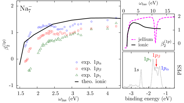
Figure 41: Top right : comparison of calculated $\beta_{2}^{(1p)}$ of ${\mathrm{Na}_{7}}^{-}$ with a jellium background and an explicit ionic one, after irradiation by a laser with $I=10^{9}$ W/cm² and $T_{\mathrm{pulse}}=60$ fs. Bottom right : experimental PES of ${\mathrm{Na}_{7}}^{-}$ irradiated by a laser of intensity $<10^{5}$ W/cm² and duration of about 10 ns [203]. Left : Experimental (open symbols, [203]) and theoretical (full curve, [128]) anisotropy parameter of the $1p$ states of ${\mathrm{Na}_{7}}^{-}$, as a function of laser frequency. $1p_{\alpha}$, $1p_{\beta}$ and $1p_{\gamma}$ correspond to state assignments of peaks observed in the experimental PES (bottom right).

All laser frequencies shown in the figure correspond to emission from the $1p$ states in the one-photon regime. The experimental data show three curves. These are associated with the three sub-peaks of the $1p$ states found in the experimental PES, see lower right panel. The theoretical calculations did not disentangle these sub-peaks and show the $\beta_{2}^{(1p)}$ from the PAD averaged over the whole $1p$ group. The theoretical and (averaged) experimental curves nicely agree with each other. For higher frequencies, we see again the smooth trend as was already observed in the example of Na₈ in Fig. 40. The data stay systematically a bit below the theoretical $\beta_{2}^{(1p)}$. This is probably due to electronic collisions not accounted for in TDLDA. The great surprise is the deep dip at low frequencies which is not an artifact because it is also clearly seen in the experimental results. It is due to a very special situation for this loosely bound anion. Indeed, we are near threshold, and the electron cloud is thus emitted with near zero momentum. The KS potential seen by the escaping electron is extremely shallow and the outgoing electronic wave function has an extremely long wavelength throughout. Thus it cannot resolve the ionic structure and the rescattering mechanism which wipes out the dips (see discussion of Fig. 40) becomes obsolete. This is demonstrated in the upper right panel of Fig. 41 where we compare $\beta_{2}^{(1p)}(\omega_{\mathrm{las}})$ for jellium and explicit ionic background over a larger frequency span. As in the case of Na₈, the jellium model produces values near 2 and a pronounced dip around 11 eV, while ionic structure delivers a generally smoother curve with a maximum around 1.5. But both, jellium and ionic background, deliver the same deep dip towards threshold. This confirms nicely that the extremely long wavelength of the outgoing electron state reduces the spatial resolution such that the soft jellium and detailed ions cannot be distinguished anymore. This is also the reason why an older calculation of $\beta_{2}$ for ${\mathrm{Na}_{7}}^{-}$ at low frequencies using a jellium model and linear response could provide realistic results [204].

In contrast to the PES which exhibits a strong dependence on laser intensity, an orientation-averaged PAD seems to be not very sensitive to it. Indeed, when irradiated by laser pulses of duration of 30 fs and frequency of 34 eV but with two different intensities ($10^{10}$ and $10^{12}$ W/cm²), the obtained PAD both delivers the same $\beta_{2}=0.38$, while the PES at the highest intensity is blurred and red shifted [190]. Note that the anisotropy parameter is here much smaller than for small Na clusters, see Fig. 43. This is again due to the influence of the ionic structure : for sodium clusters, $\beta_{2}$ decreases by about 25 % when going from jellium to ionic background. This effect should be even stronger in C₆₀, since the number of ions is much higher than for the considered Na_N with $N=3-19$. Additionally, the coupling of the electrons to the ions in carbon atoms is stronger than in simple metal clusters.

More interesting is the frequency dependence of the PAD and $\beta_{2}$. An orientation averaging procedure is applied here (see Sec. 3.4.1). We focus on the photo-emission from HOMO and HOMO$-1$ because experimentally, these are the only states which clearly emerge above the background [205, 191]. Various calculated PAD are presented in the left column of Fig. 42, and the extracted $\beta_{2}$ are plotted in the right panel.

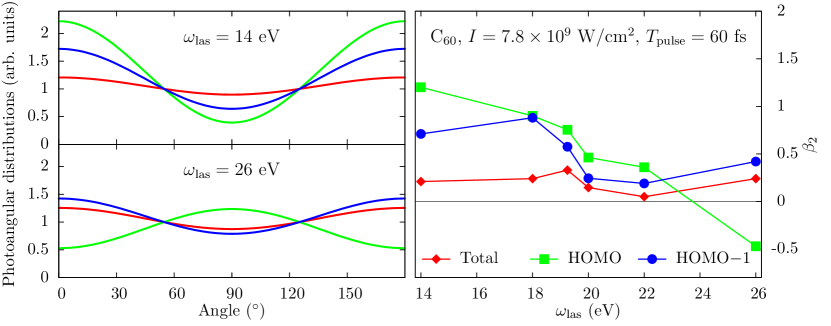
Figure 42: Left : Calculated orientation-averaged PAD from C₆₀ with radius of 6.763 a₀ irradiated by a laser pulse of intensity $I=7.8\times 10^{9}$ W/cm², duration of 60 fs, and frequency $\omega_{\rm las}$ of 14 eV (top) or 26 eV (bottom). Right : anisotropy parameter $\beta_{2}$ as a function of $\omega_{\rm las}$. Red curves: total PAD and $\beta_{2}$ from all single particle states ; light green curves : the same but from the HOMO only ; blue curves : the same but from the HOMO$-1$ only.

The total $\beta_{2}$ (black curve) does not depend on $\omega_{\mathrm{las}}$ very much. The anisotropy parameter of the HOMO and HOMO$-1$ exhibit by contrast larger variations and both states deliver different behaviors. The $\beta_{2}$ of the HOMO$-1$ (blue curve) is always positive with a minimum value at 0.18 around 22 eV. On the contrary, the $\beta_{2}$ of the HOMO (green curve) steadily decreases with $\omega_{\rm las}$ and changes of sign a bit before 24 eV. Below 22 eV, the $\beta_{2}$ of the HOMO is also higher than the one of the HOMO$-1$. The case once more demonstrates the extreme sensitivity of the $\beta_{2}$ as an observable characterizing a dynamical scenario. Mind that, in this monophoton domain, the anisotropy parameter is bound between $-1$ and $+2$, so that the variations in Fig. 42 are quite significant. Together with its strong model sensitivity (see for example the discussion on Fig. 40), this points out that $\beta_{2}$ is certainly a very rich quantity to be measured and computed in a highly refined manner.

4.4.1.4 Dependence of $\beta_{2}$ on cluster deformation

To explore the impact of cluster deformation on the PAD, we now turn to a series of small neutral and cationic metal clusters which cover planar (${\mathrm{Na}_{3}}^{+}$), prolate (Na₁₀, ${\mathrm{Na}_{11}}^{+}$), oblate (${\mathrm{Na}_{13}}^{+}$ and Na₁₈), and triaxial (Na₁₂, ${\mathrm{Na}_{19}}^{+}$) systems. We consider detailed ionic background as well as a deformed jellium approach to it. The jellium deformation is tuned in each case to reproduce the global deformation of the ionic configuration. The shape can be quantified by the quadrupole deformation $\alpha$ defined by $\alpha=\sqrt{\sum_{m=-2}^{2}\alpha_{2m}^{2}}$ with $\alpha_{2m}=4\pi\overline{r^{2}Y_{2m}}/{5NR_{\mathrm{rms}}^{2}}$, $R_{\mathrm{rms}}$ the ionic root mean square radius, $N$ the total number of ions, and $Y_{2m}$ the spherical harmonics for $l=2$. In Fig. 43, we compare $\alpha$ with the total anisotropy parameter $\beta_{2}$.

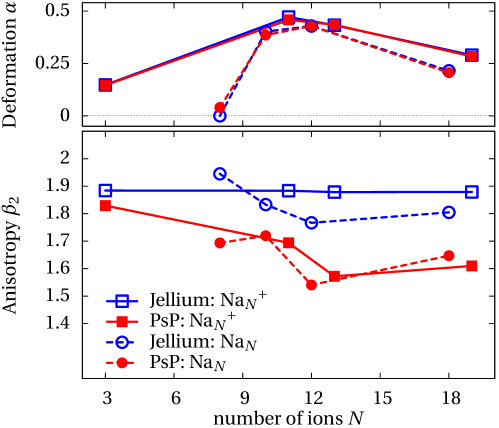
Figure 43: Comparison of quadrupole deformation $\alpha$ (top) and total anisotropy parameter $\beta_{2}$ (bottom) for small neutral (circles) and cationic (squares) clusters, obtained in a jellium description of the ionic background (open symbols) or with an explicit ionic structure (closed symbols). Adapted from [128].

As in the case of Na₈ previously discussed, $\beta_{2}$ is extracted from orientation averaged PAD, each PAD obtained after irradiation by a laser in the mono-photon regime, that is $\omega_{\mathrm{las}}=7.5$ eV for neutral species and 10 eV for cationic ones (due to a stronger binding there) with $I=10^{11}$ W/cm². The total ionization always remains between $10^{-4}$ and $10^{-3}$. We first note that $\beta_{2}$ shows only small variations, particularly for the jellium model. We cannot spot any correlation of the anisotropy $\beta_{2}$ with the deformation $\alpha$. The difference between neutral clusters and cations is also very small. However, as observed previously, there can be a large sensitivity to the structure of the ionic background. The $\beta_{2}$ is systematically smaller (more isotropic) when detailed ions are considered. It is particularly interesting to note that the discrepancy grows systematically with increasing cluster size $N$. This trend is corroborated by results from larger clusters. For example, the total anisotropy for C₆₀ comes close to zero, see Fig. 44 for low intensities. The trend complies with the interpretation that rescattering with ions enhances the isotropic background: the more scatterers, the closer to isotropy.

4.4.2 PAD in the multiphoton regime

The orientation averaged PAD in the multiphoton regime develops more detailed angular dependence as indicated by Eq. (41). For clarity, we recall it here :

$$\frac{\mathrm{d}\sigma}{\mathrm{d}\Omega}\propto 1+\beta_{2}P_{2}(\cos\vartheta)+\beta_{4}P_{4}(\cos\vartheta)+\ldots$$

In a strictly perturbative regime (low laser intensity), the series terminates at $P_{2\nu}(\cos\vartheta)$ where $\nu$ is the order of the multiphoton process which is determined by the relation of IP to photon frequency. This changes with increasing intensity where always all amounts of photons could be possible. Thus the series is, in principle, unterminated and we expect that the contributions of higher $\beta_{2n}$ increase with increasing intensity $I$. We thus briefly analyze the impact of intensity on the PAD in two emblematic cases, C₆₀ and Na₈. As we are going beyond the perturbative regime, we will consider higher $\beta_{2n}$ beyond the anisotropy $\beta_{2}$. It is to be noted that orientation averaging in the multiphoton regime has to be done explicitly by integration over orientations. Due to the high symmetry of the two test cases, only 18 integration points need to be computed.

We start with the case of C₆₀ irradiated by a laser of frequency of 1.55 eV and pulse duration of 75 fs, with the same set of increasing intensities as in use for the systematics of PES in the right panel of Fig. 37. The IP of C₆₀ being 8 eV, it requires at least 6 photons to extract electrons from occupied states. The PAD obtained in C₆₀ with different laser intensities are shown in the left panel of Fig. 44, while the first anisotropy parameters $\beta_{n}$ extracted from these PAD are plotted in the right panel.

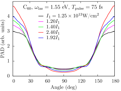
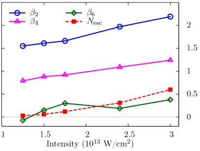
Figure 44: Anisotropy parameters of high orders (right) extracted from PAD (left) of orientation-averaged C₆₀ irradiated by laser pulses of frequency of 1.55 eV, duration of 75 fs, for different laser intensities. For the sake of completeness, the total ionization $N_{\mathrm{esc}}$ is plotted in the right panel. Adapted from [190].

The total ionization $N_{\mathrm{esc}}$ (red boxes and dashed line in the right panel) increases rapidly with $I$ as expected. The PAD shown in the left panel become more and more aligned along the laser polarization with increasing $I$. Accordingly, all $\beta_{2l}$, shown in the right panel, increase with $I$. Note that $\beta_{2}>2$ becomes possible in this non-linear regime. The limitation $-1\leq\beta_{2}\leq 2$ applies only to strict one-photon processes.

The next test case is the Na₈ cluster. Differently as in previous sections, we now run it for laser frequencies below ionization threshold, namely $\omega_{\mathrm{las}}=3.7$ and 3.9 eV while the IP is 4.4 eV. At least two-photon processes are required for ionization, probably higher ones with increasing intensity $I$. Fig. 45 shows the intensity dependence of $\beta_{2}$ (left panel) and $\beta_{4}$ (right panel).

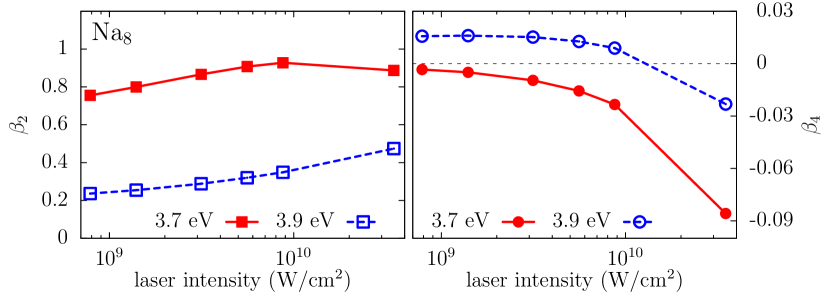
Figure 45: Anisotropy parameters $\beta_{2}$ (left) and $\beta_{4}$ (right) of Na₈ extracted from PAD with an averaging procedure over 18 orientations, after irradiation of laser pulses of duration of 60 fs and frequencies of 3.7 (red full curves) or 3.9 eV (blue dashes). Adapted from [128].

The total ionization ranges from 0.001 to 0.1, which means that all cases constitute rather moderate excitation dynamics. We see again generally an increase of total anisotropy $\beta_{2}$ with intensity. Still, the growth of $\beta_{2}$ is slower than in the previous example C₆₀ because we deal here only with two-photon processes. The next coefficient $\beta_{4}$ also shows a marked trend to larger negative values with increasing intensity. It is interesting to note that both coefficients, $\beta_{2}$ and $\beta_{4}$, are very sensitive to the laser frequency. This is also a feature of MPI while frequency dependences are more moderate for one-photon processes, see e.g. Sec. 4.4.1.2.

4.5 Impact of temperature in PES and PAD

4.5.1 Effect of ionic motion on PES and PAD

So far, the presented calculations of PES and PAD were performed at ionic ground-state configuration, i.e. at a temperature of 0 K. This ideal situation is hardly ever feasible in an experiment. Depending on the production conditions, cluster beams have temperatures in the range of several 100 K. This means that we encounter usually an ensemble of ionic configurations fluctuating around the ground-state configuration. In the following, we will discuss the impact of thermal shape fluctuations on PES/PAD.

Experimentalists are well aware of the temperature problem and have developed several techniques for dedicated cooling of cluster beams. Ion traps are particularly powerful devices for a clean handling of cluster beams [206]. We show here results from recent experiments which used a trap and cooling with a He buffer gas to produce beams of Na anionic clusters with well defined temperatures between 6 and 265 K [203]. The upper temperature is above the melting point of $\approx 250$ K for small Na clusters [207]. The test case ${\mathrm{Na}_{33}}^{-}$ is a cluster anion which has naturally a low IP. Thus one can easily realize one-photon processes with standard laser pulses. A selection of combined PES/PAD for ${\mathrm{Na}_{33}}^{-}$ is shown in the left panel of Fig. 46. The upper right panel shows the PES at different temperatures $T$ and the lower right panel the anisotropy $\beta_{2}$ as a function of $T$.

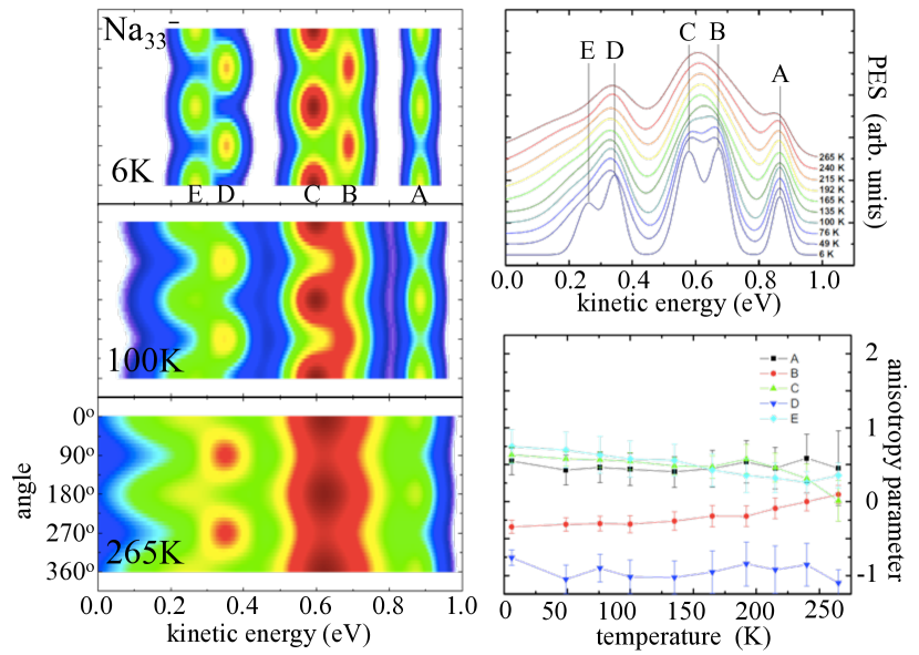
Figure 46: Left : Combined PES/PAD of ${\mathrm{Na}_{33}}^{-}$ obtained by fit of five Gaussian peaks to the raw distributions at three different ionic temperatures as indicated. Right top : extracted PES for temperatures ranging from 6 K to 265 K. Right bottom : extracted anisotropy parameter $\beta_{2}$ as a function of ionic temperature. Adapted from [203].

The PES/PAD in the left panels and the PES in the upper right panel (both analyzed at low temperature) allow one to identify five emitting states, labeled A, B, C, D, and E. The structures produced by these states in the PES (and PES/PAD) are gradually blurred with increasing temperature. This is easily understood from the fact that single-electron energies can be very sensitive to changes in the cluster shape. The thermal ensemble thus represents a more or less broadened distribution of s.p. energies which, in turn, is mapped into PES and PES/PAD. On the other hand, the anisotropies $\beta_{2}$ exhibit only a weak dependence on $T$. This probably reflects the fact that the angular momentum characteristics (stemming from their wave functions) of the s.p. states are more robust than their energies.

The numerical simulation of a thermal ensemble is conceptually straightforward, although somewhat cumbersome. One starts an ionic dynamics from the ground-state configuration by initializing ionic velocities stochastically according to a Maxwellian distribution for the given temperature $T$. This state is then propagated by TDLDA-MD for a few ps. About each 100 fs, a snapshot of the actual configuration is taken. The set of all snapshots constitutes the thermal ensemble of cluster configurations. Now, in a laser-induced dynamics propagated for each sample, the wanted observables (e.g., PES and PAD) are evaluated and incoherently superimposed. This altogether yields the observable for the ensemble. We have performed such a study for ${\mathrm{Na}_{9}}^{+}$ irradiated by laser pulses of intensity of $10^{11}$ W/cm², and FWHM of 232 fs. This pulse duration allows a high resolution of the PES peaks (see the effect of pulse duration in Fig. 34) such that line broadening comes predominantly from thermal effects. The pulse duration lies within the time scale of ionic motion. Thus the dynamical propagation is done at the level of TDLDA-MD to include properly ionic motion. For reasons of simplicity, we are not performing orientation averaging such that we see exclusively the thermal effects. The laser polarization is chosen along the symmetry axis of the $T=0$ configuration. For a first test, we use a laser frequency at 6.8 eV just below the IP. The $1s$ state ($\varepsilon_{1s}=-8.5$ eV) and degenerate $1p$ states ($\varepsilon_{1p}=-7.2$ eV) then emit through a two-photon process. We compare in Fig. 47 the PES and the PAD calculated at $T=0$ and at three increasing temperatures $T=158$, 315 and 473 K.

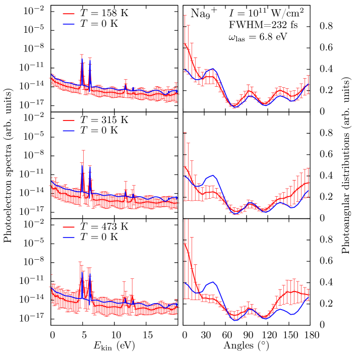
Figure 47: Left column : Photoelectron spectra of ${\mathrm{Na}_{9}}^{+}$ of fixed orientation, irradiated by laser pulses polarized along the symmetry axis of the cluster, with FWHM of 232 fs, intensity of $10^{11}$ W/cm², and frequency of 6.8 eV, at an ionic temperature $T$ of 158 K (top), 315 K (middle) or 473 K (bottom). The blue curve shows the PES at $T=0$ K. Right column : corresponding PAD.

As expected, the higher $T$, the broader the PES peaks. There is also a faint red shift of the peaks with increasing temperature. Nonetheless, it is surprising how well the structures survive in the PES even high above melting temperature (about 250 K). What the PAD is concerned, remind that it is computed without orientation averaging. It thus shows more structure and is asymmetric (reflecting the asymmetry of ${\mathrm{Na}_{9}}^{+}$). The thermal effects on the PAD are a bit larger than for the PES, but remain still small, in accordance with the experimental results for ${\mathrm{Na}_{33}}^{-}$ in Fig. 46. Fig. 47 also shows through the error bars the uncertainty associated with thermal fluctuations. These are computed in standard manner as the variance of PAD and of the logarithm of the PES yield from the statistical ensemble. The uncertainties grow with temperature. They stay rather small for the PES, showing once more that these structures are rather robust. The error bars are larger for the PAD in forward (0^∘) and backward (180^∘) direction. Fortunately, these forward and backwards cones have a small integration weight, such that global measures as, e.g., the anisotropy $\beta_{2}$ are again robust.

We now concentrate on the case of $T=315$ K and complement the $\omega_{\mathrm{las}}=6.8$ eV by two other frequencies : one smaller with 3.4 eV well below IP and one larger with 13.6 eV well above IP. The laser polarization and duration are the same as before. The intensity is $10^{11}$ W/cm² for the two lower $\omega_{\mathrm{las}}$ and $10^{12}$ W/cm² for $\omega_{\mathrm{las}}=13.6$ eV to deliver comparable ionization for all cases. Fig. 48 shows the resulting PES and PAD (again compared with the $T=0$ case).

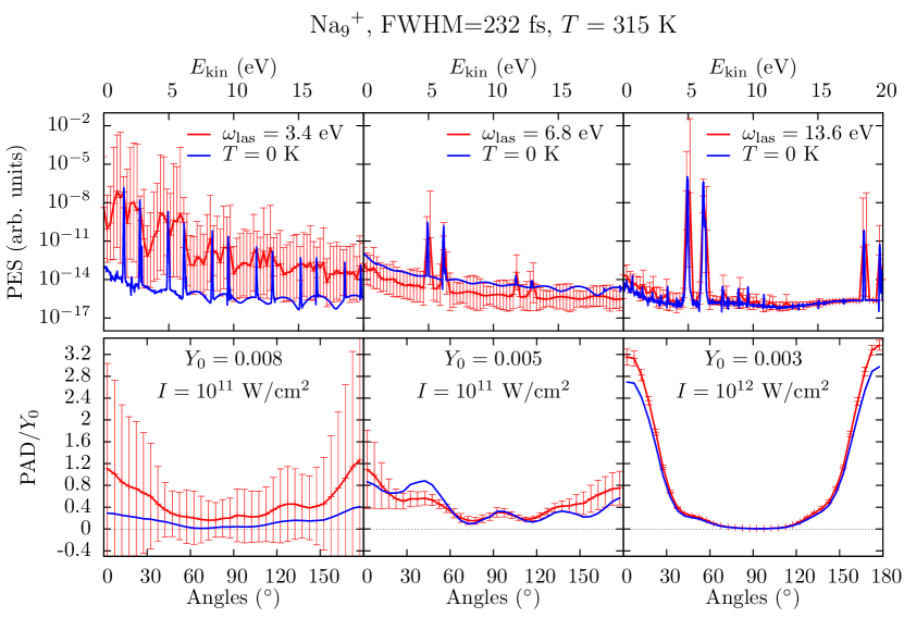
Figure 48: Top row : Photoelectron spectra of ${\mathrm{Na}_{9}}^{+}$ with initial ionic temperature of 315 K, irradiated by laser pulses of FWHM of 232 fs, intensity of $10^{11}$ W/cm², and frequency of 3.4 eV (left), 6.8 eV (middle), and 13.6 eV (right). The blue curve shows the PES at $T=0$ K. Bottom row : corresponding PAD.

For the highest frequency (right panels), the impact of temperature is quite weak: we still observe a slight broadening of the peaks in the PES. However, the effect on the PAD is negligible. This result is intuitive because for such a high laser frequency, the photoelectrons are extracted by absorption of a single photon and basically follow the laser field, as is visible from the fact that the PAD is peaked along $\vartheta=0^{\circ}$ and $180^{\circ}$. On the contrary, the lowest frequency (left panels) lies deeply in the multi-photon regime. And the uncertainties produced by the ionic motion at this temperature are extremely large. Apart from that, MPI peaks are still visible in the PES, although much broadened. At the side of the PAD, the uncertainties are larger than the signal. This means that in the multi-photon regime, the PAD is very sensitive to ionic temperature. The intermediate frequency (middle panels) lies in between in all respects. Temperature effects are already well visible, but not as disastrous as for low frequency. This example shows that the ionic temperature should better be well controlled and kept at a sufficiently low value to allow a quantitative analysis of PAD.

4.5.2 Impact of electronic dissipation on PES and PAD

In Sec. 4.3.4, we found that a smooth exponential PES develops for sufficiently high intensities, see Fig. 37. Figure 10 did also show a series of exponential PES from a measurement with high intensities (fluences) and a long pulse. The question is to what extent this could be a signature of thermal emission after full thermalization of the cluster.

We start the discussion with looking back at Fig. 37. From the inverse slope of the exponential, we would read off an apparent temperature of $T_{\rm app}=1.4$ eV. From the TDLDA calculations, we also find that the energy deposited by the laser pulse in the cluster is about $E^{*}\simeq{1.8}$ eV. Assuming that all this energy is converted into thermal energy would lead to an intrinsic temperature of about $E^{*}/160\simeq{0.01}$ eV which is two orders of magnitude smaller than $T_{\mathrm{app}}$. This, together with the fact that TDLDA does not account for electronic thermal effects, clearly rules out the thermal origin of the observed exponential slope.

The experimental results from [47] in Fig. 10 (see Sec. 2.3.1) did show also a remarkable series of smooth exponential PES.

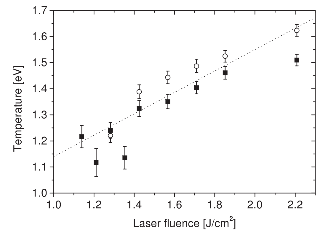
Figure 49: Experimental apparent electronic temperature as a function of laser fluence as extracted from PES for C₇₀ (squares) and C₆₀ (circles). The dotted line is a fit to the temperatures vs laser fluence obtained in the case of C₆₀ in [52]. Note that the laser fluence has an overall systematic uncertainty of 10%, which is not included in the present error bars. From [47].

Fig. 49 gathers the apparent temperatures (inverse slopes) extracted from these PES. Again we find rather large values in the range from 1 up to 1.6 eV, near the 1.8 eV of the previous example. The remaining excitation energy is not available for these experiments. Nevertheless, it is questionable that these exponential slopes should correspond to real temperatures of the system in thermal equilibrium. This is why one wisely has coined the notion “apparent temperature” for the slope of the PES, see Fig. 10 from [47]. The example of Fig. 37 has shown that a smooth exponential pattern can also be explained by TDLDA calculations. In fact, the exponential profile can be nicely fully explained in terms of multiphoton perturbation theory [50]. Any MPI yields an exponentially decreasing slope. The Coulomb shift increasing with ionization stage increasingly washes out the MPI peaks to yield eventually a purely exponential PES.

In order to check how far pure TDLDA (free of any thermalization) can describe exponential PES, we consider ${{\rm Na}_{93}}^{+}$ for which calculations can be compared with experimental data. In this experiment both total ionization and PES have been measured. The exponential shape of the PES was attributed to thermal effects [208]. The resulting apparent temperature (inverse slope) and total ionization are plotted as a function of laser intensity in Fig. 50.

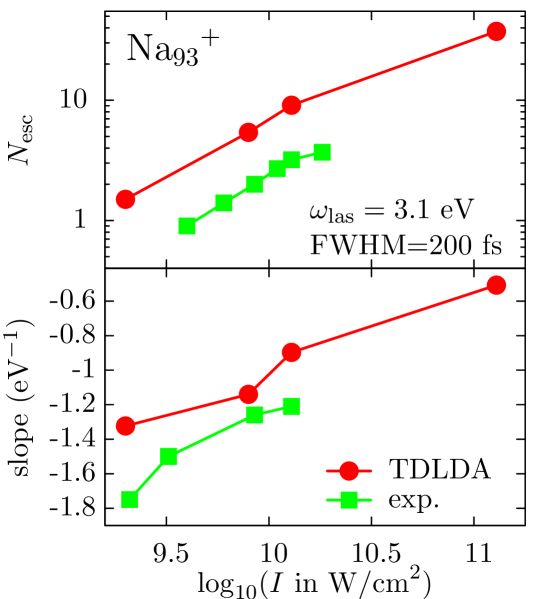
Figure 50: Ionization characteristics of ${{\rm Na}_{93}}^{+}$ irradiated by lasers of increasing intensities (in W/cm²) but fixed photon frequency at 3.1 eV and pulse FWHM at 200 fs. Calculations (red circles) are compared to experimental data (green squares) from [208]. Ionic dynamics has been included with a Maxwellian distribution of velocities according to a temperature of 100 K. Upper panel: total ionization in logarithmic scale. Lower panel: slope of the PES. Adapted from [50].

The experimental results are compared to standard TDLDA calculations performed under the same laser conditions. The theoretical results are surprisingly close to the data, which indicates that a purely thermal interpretation is not compelling. Consider the apparent temperatures (inverse of the slopes). They are in range 0.7–2 eV for TDLDA and 0.6–0.8 eV for the experiment. This would amount to about 300 eV intrinsic energy in case of full thermal equilibrium ($\approx$150 eV if only electrons were thermalized) : this is too much as compared to the typical cluster binding in ${{\rm Na}_{93}}^{+}$. Thus we are surely far from full thermalization in this case. On the other hand, there are small, but systematic, differences which may be a trace of thermal effects. The apparent temperature (lower panel) and the ionization (upper panel) is somewhat lower in the data than in TDLDA. This indicates that the data represent, in fact, a mixed situation, not fully thermalized yet, but somewhere on the way.

There still remains the task to distinguish direct from thermal electron emission. We have argued above that exponential PES are only a necessary condition, not a sufficient proof. Additional information for a better discrimination is delivered by the PAD. Isotropic PAD are another necessary, usually much more conclusive, condition for thermal emission. For example, the experimental PES/PAD in Fig. 24 shows a larger inner spot of isotropic emission at low energies which can be associated with thermal electrons. At the theoretical side, a relevant description of thermalization requires dynamical correlations beyond TDLDA. This has been achieved at the semi-classical level, see Sec. 4.5.3. It is still a great challenge for a fully quantum mechanical modeling, see Secs. 5.2.2 and 5.2.3. In the following, we will briefly present a simple estimate for the contribution of thermal electrons which provides at least a first impression of the impact of thermal electrons on PAD.

The case of C₆₀, illustrated in Fig. 51, addresses the complementing PAD signal, which is expected to contain a significant isotropic component if strong thermal effects are present.

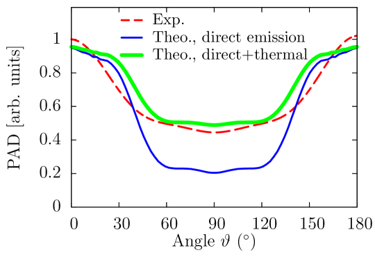
Figure 51: Comparison of experimental photoangular distribution from C₆₀ HOMO and HOMO$-1$ states (red dashed curve) in the multiphoton regime with total theoretical PAD. One calculation takes into account only direct electronic emission (blue thin line) and the other one includes an estimate of the additional thermal component due to electronic temperature (green thick line), see text for details. From [191].

We consider here the MPI regime, irradiated by a laser of frequency 1.55 eV, pulse FWHM of 20 fs and intensity of $1.25\times 10^{13}$ W/cm². The experiments deliver a PAD energy-integrated over the HOMO, HOMO$-1$, and HOMO$-2$ and the theoretical results are integrated over the same interval [191]. Although both results have similar pattern, the TDLDA distribution is much more anisotropic than the experimental one. This reflects once again the fact that TDLDA underestimates electron-electron collisions which are the doorway to thermal effects. It is thus interesting to test whether thermal effects might explain the observed discrepancy. For a simple estimate, we proceed as follows. We assume that the residual electronic excitation energy which is found to be 1.8 eV is fully thermalized. Thermal energy is later on converted into a thermal electronic emission. The IP of C₆₀ is 7.8 eV. The 1.8 eV excitation energy thus suffices to emit about 0.22 electrons (when neglecting the possible C₂ dissociation channel which requires larger energy). We then add up the contribution of the extra 0.22 emitted electrons as a thermal, isotropic background to the PAD. This leads to the curve labeled “direct$+$thermal” in Fig. 51, which now agrees fairly well with the experimental curve. Of course, the reasoning basically provides an argument and does not constitute a theory by itself, but it once again confirms that bare TDLDA underestimates electronic collisions, while they are obviously non negligible in the MPI regime.

4.5.3 The semi-classical route

As already discussed in Sec. 3.5, thermal effects in finite systems can presently only be attained via a semi-classical approximation, leading to semi-classical kinetic equation such as VUU. The underlying Vlasov equation is the semi-classical limit of TDLDA. VUU employs additionally the Uehling-Uhlenbeck collision term which accounts for the dynamical electron-electron correlations. Ionization, as a basic dynamical mechanism, has been discussed within VUU in several papers [209, 210, 60, 169, 141]. The interesting point for the present discussion is to analyze the impact of VUU as compared to Vlasov. We shall discuss the point on the example of ${{\rm Na}_{41}}^{+}$. We fix the pulse duration at a FWHM of 25 fs. We consider two laser intensities, $10^{11}$ W/cm² and $6\times 10^{11}$ W/cm², and three frequencies, $\omega_{\mathrm{las}}=2.7$, 3.0, and 3.3 eV, around the plasmon frequency of the system (3 eV). The time evolution of the ionization is shown in Fig. 52.

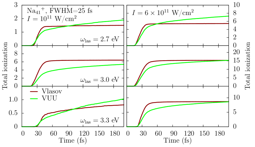
Figure 52: Comparison of the time evolution of the total ionization in Vlasov (brown lines) and VUU (light green lines) approaches. The system is ${{\rm Na}_{41}}^{+}$ irradiated by lasers of cos² profiles with FWHM of 25 fs. Intensities are 10¹¹ (left panels) and $6\times 10^{11}$ W/cm² (left panels). Frequencies are varied between 2.7 and 3.3 eV, which covers the dominant optical response peak located around 3 eV for this system.

It strongly depends on $\omega_{\mathrm{las}}$, as expected at the passage of a resonance [211]. The most interesting feature is the shape of the emission profile. In the Vlasov calculations, ionization grows very quickly in the early stages and levels off once the laser pulse is switched off. Note that the huge ionization blue-shifts the plasmon resonance such that the case $\omega_{\rm las}=3$ eV becomes off-resonant and subsequently emission is terminated after the pulse (see Sec. 4.2.1). The VUU results look much different. Emission is suppressed in early stages. This is overcompensated by a steadily continuing emission later on. The pattern are very similar for all three laser frequencies, while the amplitude of the effect (and the relative values of Vlasov and VUU ionization at early times) depends sensitively on frequency. This is a long known effect that field amplification by the plasmon resonance naturally leads to enhanced emission [212] in TDLDA and correspondingly in Vlasov [211, 210]. VUU shows the same resonant behavior, but modulates the time profile of emission. It reduces ionization in early stages because electron-electron collisions remove energy from the direct emission channel, and it enhances emission in later stages by releasing gently the stored energy.

The analysis of PES is of limited interest in Vlasov and VUU as at low energy neither can identify electron single particle energies because of their semi-classical nature. The obtained PES are thus always more or less exponentially decreasing, whatever the laser conditions. More interesting is the PAD which can be easily evaluated in Vlasov and VUU and which does not suffer so much from the semi-classical approximation. Furthermore, it is an ideal observable to identify thermal effects in terms of isotropy of the PAD, as we have seen in Sec. 4.5.2. The point is illustrated in Fig. 53 for the same test case as in Fig. 52, and for a few laser frequencies, again around plasmon frequency of ${{\rm Na}_{41}}^{+}$.

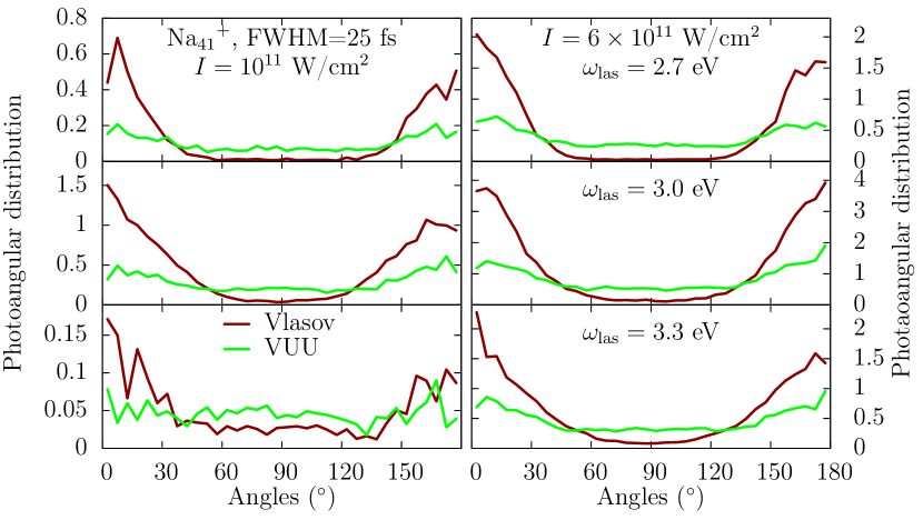
Figure 53: Comparison of angular distributions in Vlasov (brown lines) and VUU (light green lines) approaches. Same system and laser conditions as in Fig. 52.

Orientation averaging has not been performed, which is an acceptable approximation here because ${{\rm Na}_{41}}^{+}$ is large and close to sphericity. For all laser frequencies, the PAD from Vlasov exhibit strongly oriented emission along the laser polarization. The effect becomes larger when $\omega_{\mathrm{las}}$ comes closer and closer to the plasmon frequency. This is again a consequence of field amplification near the resonance. A similar trend with frequency is observed in the VUU calculations, although less pronounced. More striking is the fact that the PAD from VUU are much less peaked than the Vlasov ones. Very clearly, the VUU results have a strong isotropic component. The effect is especially clear far from the plasmon resonance but remains very visible close to it. We observe then a competition between field amplification (from resonance) and thermalization [211]. In any case, we see a significant enhancement of ionization perpendicular to the laser polarization, as compared to Vlasov, a clear signature of isotropy.

5 Future directions

We have seen in the previous sections the richness and variety of observables today accessible in experiments and theory. Of course, there remain many open questions for future research. We want to illustrate in this section two lines of development which we consider as especially promising and which require dedicated efforts both from the experimental and theoretical side.

The first aspect again focuses on the analysis of dynamics in terms of PES and PAD from which we have seen that it is a powerful tool. We will now consider the analysis in terms of PES and PAD in connection with the short pulses delivered by a bypassing ionic projectile. As we shall see, PES and PAD can again provide useful insights into the underlying dynamics.

The second topic concerns electronic thermalization which was already addressed to some extent in Sec. 4.5.2. The excitation energy deposited originally by the laser pulse is released in the first stages of the dynamics by direct electron emission. However, part of the deposited energy is progressively converted into incoherent electronic excitation of ”thermal” nature. This takes place on a moderate time scale of some tens of fs. Analysis of such effects is difficult and requires detailed experiments (see Figs. 10 and 49). From the theoretical point of view, the situation is even worse as it requires the development of deep extensions of available current theories such as real-time TDDFT. In the following, we address both these directions in more detail.

5.1 An excursion into irradiation by charged projectiles

We briefly discuss in this section PES and PAD of ”photo”-electrons emitted after collision with a fast charged projectile. We put the word ”photo” in quotation marks because the electromagnetic pulse has not a well defined frequency here. Although rare, there exist data measured on atoms and mono-atomic dimers with a special focus at very high kinetic energies ($E_{\rm kin}>40$ eV) of the projectiles. This was first motivated by the observation of non-monotonous patterns in the PES after irradiation of O₂ and N₂ with photons in the 30–60 eV range [213], which were explained theoretically one year later [214] by Young-type interferences between electronic wave functions of electrons coherently emitted from identical atomic centers. Various experiments have been performed on H₂ bombarded by He⁺ and He²⁺ of 20 and 40 keV [215] or by 8 keV electrons [216, 217], on N₂ colliding with 1–5 MeV H⁺ [218], and on O₂ colliding with 3.5 MeV/$u$ C⁶⁺ ions [219] or 30 MeV O⁵⁺ and O⁸⁺ ions [220]. Very recently, collisions of 3.5 MeV/$u$ C⁶⁺ ions on uracile [221] and of 4.5 MeV/$u$ O⁸⁺ ions on H₂O [222] have been reported. The kinetic energy of the ejected electrons ranges from a few eV up to 600 eV, and the emission is measured between 20^∘ and 150^∘.

The pulses from fast projectiles are extremely short and cover a very broad band of frequencies. At first glance, this looks like a disadvantage as there is thus no specific frequency information in the pulse. However, it has the advantage that it enables to extract unambiguously effects from the system’s modes. To illustrate this point, we start with two pedagogical examples which have a dominant dipole mode, namely the case of Na₂ and Cs₂. The Na₂ is described by explicit ions and pseudopotentials, while we use a deformed jellium background for the description of Cs₂. The interaction of the irradiated system with a very fast charged projectile can be modeled by an instantaneous boost of the electronic wave functions at $t=0$ [148]. Note that this procedure is the same as the one we use for the calculation of an optical response, see Sec. 4.1.2. More precisely, we apply a boost $\mathbf{p}$ to each occupied s.p. wave function $\varphi_{j,{\rm gs}}$ of the ground state, and take the obtained wave functions as the initial states :

$$\varphi_{j}(\mathbf{r},t\!=\!0)=\exp(\mathrm{i}\mathbf{p}\cdot\mathbf{r})\varphi_{j,\mathrm{gs}}(\mathbf{r})$$ (56)

This mimics the effect of the Coulomb field caused by a fast by-passing charged projectile. For simplicity, let us consider a boost in the $z$ direction only. If the projectile is fast enough, we can assume that it travels on a straight line with constant velocity $v_{\rm proj}$. Therefore, one can evaluate the net force integrated over the collision, and the latter exhibits a component only in direction to the point (here the $z$ axis) of closest impact [223]. The induced boost for a projectile of charge $Z$ and an impact parameter $b$ then reads

$$p=\frac{4Ze^{2}}{bv_{\rm proj}}\quad.$$ (57)

One can see that, for a given value of the boost, larger $b$ and/or $v_{\rm proj}$ can be compensated by increasing the charge $Z$ of the projectile. To derive Eq. (57), the passage time of the projectile, which reads $b/v_{\rm proj}$, should be much smaller than a typical electron reaction time $\omega_{\mathrm{el}}^{-1}$. If one uses the value $\omega_{\mathrm{el}}=1$ Ry and an impact parameter $b=10$ a₀ for a rough estimate, we have the constraint $v_{\rm proj}\gg b\omega_{\rm el}=200$ a₀/fs. This lower value corresponds to a kinetic energy of 700 keV for a colliding proton. Inserting this value of $v_{\rm proj}$ in Eq. (57) with $b=10$ a₀ and $Z=1$ yields a maximal value ${}_{\rm max}=0.08$/a₀, which is in the range of the boosts used in the following.

We now come back to the first two test cases that we have studied, namely Na₂ and Cs₂. Both systems exhibit a very clean plasmon peak at 2.1 eV and 1.4 eV respectively. Fig. 54 shows the obtained PES.

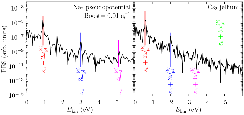
Figure 54: Photoelectron spectra of Na₂ described by pseudopotentials (left) and Cs₂ described by a jellium background, excited by an instantaneous boost of 0.01 a${}_{0}^{-1}$ applied to the wave functions at $t=0$. The vertical lines are positioned at energies corresponding to the single particle energy of Na₂ (of Cs₂), $\varepsilon_{a}=-3.23$ eV ($\varepsilon_{b}=-2.18$ eV), blue-shifted by multiples of the plasmon frequency $\omega_{\rm pl}^{(a)}=2.1$ eV ($\omega_{\rm pl}^{(b)}=1.4$ eV).

On top of the exponential decrease emerge some peaks. One can identify the dominant ones as multi-plasmon excitations, similar to those already discussed in Sec. 4.3.5.1 : the energy given by the boost to the system is mainly stored in the dominant dipole mode, let us call it for simplicity the “plasmon”. Since the plasmon frequency is below the ionization threshold for each case, two or more plasmons are needed in order to ionize the system. And indeed, the double and triple plasmon processes are clearly visible in the PES. It becomes more difficult to disentangle higher orders from the background.

We now turn to a more involved case, that is the C₅ chain. It is described by an explicit ionic structure and the 20 valence electrons are shared among 8 different electronic levels. Note that the HOMO$-2$ and HOMO$-3$ are doubly degenerated. We distinguish longitudinal modes along the symmetry axis (elongated direction) and transversal modes perpendicular to it. The transversal optical response (not shown here) is suppressed by more than one order of magnitude with respect to the longitudinal response and it is substantially fragmented. Therefore, we do not expect that the peaks in transversal modes can significantly contribute to the PES. We concentrate the following discussion only longitudinal modes. The photoabsorption spectrum of C₅ in this direction is dominated by one single, strong and sharp resonance at $\omega_{\mathrm{pl}}=6.5$ eV. The notion plasmon is justified here because this is a truly collective oscillation in the sense of a Mie surface plasmon. The left panel of Fig. 55 shows the total PES stemming from all states, and the state specific PES of the HOMO (state 8), HOMO$-1$ (state 7) and HOMO$-2$ (state 6).

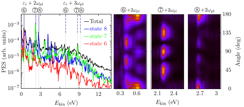
Figure 55: Electron emission from C₅ chain after excitation by an instantaneous boost of 0.07 a${}_{0}^{-1}$ along the chain direction of the electronic wave functions at $t=0$. Left panel : PES (in the longitudinal direction) of all states (black), of the HOMO (state 8, blue), HOMO$-1$ (state 7, green), and HOMO$-2$ (state 6, red). The vertical lines indicate the 2- and the 3-plasmon processes from these three least bound states, with a Coulomb shift (see Sec. 4.3.4) of 0.3 eV applied to account for the total ionization of 0.066 at the end of the simulation time. Right : Density maps of combined PES/PAD focused in the 2-plasmon excitation energy window of states 6, 7, and 8 respectively. The angle is measured with respect to the chain direction.

The dominant peaks at low energies can be clearly identified as 2-plasmon excitations from states 6, 7, and 8, which are emphasized by vertical lines. The state-resolved PES confirm this interpretation. For instance, the peak in the total PES at 2.3 eV comes from the PES of state 7 (green curve). The same occurs in the two other peaks for states 6 and 8 excited by 2-plasmon processes. As for the 3-plasmon peaks, one can catch some of the peaks, especially that of state 7. We also observe other peaks which are most likely images of the s.p. spectrum but for frequencies different from the plasmon one. In contrast to a frequency-selective laser pulse, the boost excites here all possible modes. Due to the strength of the excitation, there might also be some cross-talk to the transverse modes. It is therefore expected that the present phenomenon can only be seen in systems with a rather ”clean” dipole response characterized by sharp plasmon resonances in all directions and not too much a fragmented spectrum.

The right panels in Fig. 55 display the full combined PES/PAD zoomed onto the features corresponding to the doubly and triply excitations from states 6, 7, and 8. The angle is measured with respect to the longitudinal direction of C₅. The striking feature is that, although the boost is performed along the chain, the electrons are not exclusively emitted in this direction. For instance, states 6 and 8 exhibit in addition a sizable emission at 60^∘ and 120^∘. On the contrary, state 7 preferentially emits at 45^∘, 90^∘ and 135^∘. Clearly, these combined PES/PAD allow one to relate the emission behavior to the symmetry of the depleted wave functions as in cases with lasers, see e.g. Fig. 46.

5.2 Towards quantum dissipative electron dynamics

5.2.1 From VUU to quantum world

Although VUU (see Sec. 4.5.3) provides a way to describe dissipation in dynamical scenarios, it is limited to large excitation energies and to simple materials as, e.g., alkaline clusters. Both limitations are direct consequences of the semi-classical nature of VUU. Simple metals can be described because their electron cloud comes close to a Fermi gas. Reducing the excitation energy or considering other systems (as e.g. C₆₀) requires to account for quantum effects which renders VUU inapplicable.

This calls for a quantum kinetic theory. This can be seen two ways, either as quantum counterparts of the VUU equation (47) or as TDLDA complemented by a quantum generalization of the UU collision term (48). Anyway, such a theory deals with impure quantum states which are described at the level of the one-body density matrix . The corresponding dynamical equation for $\hat{\rho}$ reads

$$\mathrm{i}\frac{\partial\hat{\rho}}{\partial t}=[\hat{h},\hat{\rho}]+I_{\mathrm{coll}}[\hat{\rho}]\quad.$$ (58)

The commutator with the mean-field Hamiltonian $\hat{h}$ describes the mean-field evolution according to TDLDA. It is complemented by a collision term $I_{\mathrm{coll}}[\hat{\rho}]$ which, however, becomes awfully involved in the quantum case [224]. There does not yet exist any routine solution to the problem in finite systems, in spite of the many investigations, particularly in nuclear physics [58, 135, 225]. So far, most practical solutions rely on a (partial or full) semi-classical treatment [58]. The many detailed experiments on cluster dynamics discussed in the previous sections revive the call for a manageable quantum kinetic theory. We discuss in this section two promising directions of research along that line.

5.2.2 A relaxation time ansatz

VUU in the semi-classical domain and stochastic TDHF/TDLDA (see Sec. 5.2.3) describe dissipation in a very detailed, thus expensive, manner. In cases of moderate fluctuations, the system as such remains intact and the outcome is rather obvious : the dissipative dynamics drives steadily towards thermal equilibrium of a still compact system. This suggests a simplification in terms of the relaxation-time approximation which had been used since long in the homogeneous electron gas [65]. An implementation for finite fermion systems had been proposed in the nuclear context in [226]. But the computational limitations at that time did not allow realistic applications. Just recently, we have taken up this old idea of a relaxation time approximation and started to implement for cluster dynamics. We give here a brief preview of this ongoing work.

The relaxation-time approximation starts from Eq. (58). The collision term $I[\hat{\varrho}]$ is approximated by

$$\mathrm{i}\partial_{t}\hat{\varrho}-\left[\hat{h},\hat{\varrho}\right]=\frac{1}{\tau_{\mathrm{relax}}}\left(\hat{\varrho}-\hat{\varrho}_{\mathrm{equil}}\left[\rho(\mathbf{r}),\mathbf{j}(\mathbf{r})\right]\right)\quad.$$ (59a)

The right-hand-side is the effective collision term which forces the system to converge towards the equilibrium. Note that this employs the local equilibrium $$\hat{\varrho}_{\mathrm{equil}}[\rho(\mathbf{r}),\mathbf{j}(\mathbf{r}),E] E \hat{\varrho}(t)$$ which depends on the instantaneous local density, current and energy from the given . It reads

$$\hat{\varrho}_{\mathrm{equil}}=\sum_{\alpha}|\varphi_{\alpha}\rangle n_{\alpha}^{\mathrm{(equil)}}\langle\varphi_{\alpha}|\quad,\quad n_{\alpha}^{\mathrm{(equil)}}=\frac{1}{1+\exp((\varepsilon_{\alpha}-\epsilon_{\mathrm{F}})/T)}$$ (59b)

and can be computed with density- and current-constrained TDLDA [227, 228]. The temperature $$T E \tau_{\mathrm{relax}}$$ is tuned iteratively such that the total energy matches the wanted value . The key parameter is the local relaxation time for which we need a reliable choice. To that end, we recur to a semi-classical estimate of relaxation time [229, 230, 231, 232]. It is based on the Fermi gas model in which the relaxation time becomes simply

$$\frac{\hbar}{\tau_{\rm relax}}=\frac{16}{15}\frac{m}{\hbar}\sigma_{\mathrm{ee}}T^{2}\quad,$$ (59c)

where $k_{B}=1$ and $\sigma_{\mathrm{ee}}$ is the effective in-medium cross section for electron-electron collisions. For metal clusters, we find $\sigma_{ee}\approx 4\pi r_{s}^{2}$ [209]. Eqs. (59) together constitute the dissipative TDLDA in relaxation-time approach.

Fig. 56 shows a first result from the newly developed dissipative TDLDA scheme.

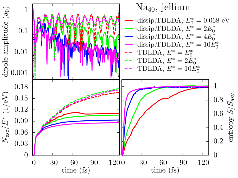
Figure 56: Time evolution of basic observables in Na₄₀ with soft spherical jellium background (12) using $r_{s}=3.65$ a₀ and $\sigma_{\mathrm{jel}}=1$ a₀, after instantaneous boost with corresponding excitation energy $E^{*}$ as indicated : Ionization $N_{\mathrm{esc}}$ normalized to $E^{*}$ (bottom left), envelope of the dipole signal (top left), and single particle entropy $S$ normalized to the asymptotic entropy $S_{\mathrm{asy}}$ (bottom right). Compared are results from pure TDLDA (dashes) with those from TDLDA with dissipation in relaxation-time approximation (full curves).

We consider as a test case Na₄₀ after instantaneous boost of its electron cloud at various boost energies. The s.p. entropy $S=\sum_{\alpha}\left(n_{\alpha}\log{n}_{\alpha}+(1-n_{\alpha})\log(1-n_{\alpha})\right)$ is shown on the right panel. It demonstrates most clearly the evolution towards thermal equilibrium. The global relaxation time shrinks visibly with increasing excitation. This is a general feature already well known from VUU. It is related to the fact that the phase space for transition opens up with increasing energy. The relaxation times deduced from this figure range from about 40 fs for low excitation down to few fs for very energetic cases. This is in range of measured values [159, 233]. The time evolutions of the dipole envelope (top left) from pure TDLDA (dashed lines) are only very slowly decaying and look at the scale of this figure nearly constant. Activating dissipation leads to a clear decay of the signal : the higher the excitation, the stronger the decay (in accordance with the right panel). But note that this decay starts only after some delay while the evolution in the early stages is very similar to TDLDA. Finally, the left lower panel shows the time evolution of ionization. The ongoing dipole oscillations in case of TDLDA leads to ongoing electron emission. The case with dissipation shows a leveling off for the ionization. The dipole signals has been damped away and the excitation energy is converted to intrinsic, thermal energy. This energy later on leads to a thermal electronix emission at a much slower time scale, thus not visible here. After all, we see that dissipative TDLDA can provide a pertinent of the thermalization of an excited electron cloud.

5.2.3 Stochastic Time-Dependent Hartree-Fock

An alternative route to kinetic theory is provided by stochastic methods describing the system as an ensemble of (pure) mean-field states. This leads to Stochastic Time-Dependent Hartree-Fock (STDHF), or Stochastic TDLDA (STDLDA) when combined with density functionals. It was originally formulated in the context of nuclear collisions [234], whence the acronym TDHF, but it can formulated for whatever system in which a quantum mean field provides a sound description of the ground state and to low energy properties. In the case of clusters and molecules TDLDA provides the obvious effective mean field theory as a starting point, thus coming to STDLDA. For simplicity, we will use the notion STDHF further on. STDHF contains all the ingredients of a standard kinetic equation, complemented by proper statistical fluctuations. It accounts for collisional correlations (from electron-electron collisions). They are treated in incoherent manner and should not be mixed with coherent correlations as they typically dominate in low-energy processes.

The original formulation of STDHF started from the quantum Liouville equation for density matrices. The early studies could show that the ensemble description of STDHF can be reduced to a quantum Boltzmann equation complemented by a to the quantum Boltzmann Langevin equation [234]. The latter was introduced in [235, 236] and has been particularly studied in the nuclear context [237, 238, 225, 239]. STDHF is thus a well founded theory containing all the ingredients necessary for a description of dissipative electronic features. It has unfortunately never been explored at full quantum level because of its complexity. It is only recently that the first calculations were performed in model systems [240] with a proper reformulation of the theory. The first results are quite promising and we will thus discuss here briefly the formalism and typical results obtained in a simple system.

The STDHF describes the system by an ensemble of $\mathcal{N}$ Slater states $\{|\Phi^{\alpha}\rangle,\alpha=1,\ldots,\mathcal{N}\}$. Each state $|\Phi^{\alpha}\rangle$ is associated with a set of single-particle (s.p.) states $\{\varphi^{\alpha}_{i},i=1,\ldots,\Omega\}$. The labels $i=1,\ldots,N$ with $N<\Omega$ stand for the occupied (hole) states. We also include in the description a sufficient amount of unoccupied (particle) states $i=N\!+\!1,,\ldots,\Omega$ which will serve as a ”reservoir” of levels for transitions to come. With this ensemble of s.p. states we can now unfold hierarchy of $n$-particle-$n$-hole ($nph$) excitations. The first ones to be appear are $2ph$ excitations because $1ph$ excitations are already accounted for in the mean-field propagation (TDHF or TDLDA). The correlated wave function (starting from an uncorrelated situation) can then be expanded as

$$|\Psi^{\alpha}(t)\rangle=|\Phi^{\alpha}(t)\rangle+\sum_{pp^{\prime}hh^{\prime}}c^{\alpha}_{pp^{\prime}hh^{\prime}}(t)|\Phi^{\alpha}_{pp^{\prime}hh^{\prime}}(t)\rangle\quad,\\$$ (60)

with

$$|\Phi^{\alpha}_{pp^{\prime}hh^{\prime}}\rangle=\hat{a}_{p}^{\dagger}\hat{a}_{p^{\prime}}^{\dagger}\hat{a}_{h^{\prime}}^{\mbox{}}\hat{a}_{h}^{\mbox{}}|\Phi^{\alpha}\rangle.$$ (61)

Note that the $2ph$ states $|\Phi^{\alpha}_{pp^{\prime}hh^{\prime}}\rangle$ are also Slater states. Starting from an uncorrelated situation, one then propagates a correlated state $|\Psi^{\alpha}(t)\rangle$ up to a certain time $\tau$ at which it is sampled in terms of an ensemble $\{|\Phi^{\alpha}_{\kappa}\rangle,w^{\alpha}_{\kappa}\}$, where $\kappa\in\{0,pp^{\prime}hh^{\prime}\}$. The weight $w^{\alpha}_{\kappa}=|c^{\alpha}_{pp^{\prime}hh^{\prime}}|^{2}$ is the probability with which $|\Phi^{\alpha}_{\kappa}\rangle$ appear. It is evaluated by means of time-dependent many-body perturbation theory which finally leads to a transition probability following Fermi’s golden rule as [234]

$$w^{\alpha}_{pp^{\prime}hh^{\prime}}=\tau\left|\langle\Phi^{\alpha}_{\kappa}|\hat{W}|\Phi^{\alpha}\rangle\right|^{2}\delta(\varepsilon^{\alpha}_{p}\!+\!\varepsilon^{\alpha}_{p^{\prime}}\!-\!\varepsilon^{\alpha}_{h}\!-\!\varepsilon^{\alpha}_{h^{\prime}})\quad,$$ (62)

where we have introduced the residual interaction $\hat{W}$ complementing the mean-field hamiltonian $\hat{h}$. The original state $|\Phi^{\alpha}\rangle$ itself has a weight $w^{\alpha}_{0}=1-\sum w^{\alpha}_{pp^{\prime}hh^{\prime}}$ (attributing $w^{\alpha}_{0}$ to the ”no transition” case) which is the complement of all the other transition probabilities. The Dirac $\delta$-function has to be taken with a word of caution. The full expression involves an operator $\delta$ function of the mean-field Liouvillean [234]. The approximation (62) involves s.p. energies taken as expectation values over the s.p. states. These, however, are ambiguous to the extent that one has always the freedom of a unitary transformation amongst the occupied states. We define the $\varepsilon^{\alpha}_{i}$ uniquely by diagonalizing the actual mean-field hamiltonian $\hat{h}^{\alpha}$ separately amongst occupied states and unoccupied states. In practice, the Dirac $\delta$-function has to be augmented by a finite width to account for the discrete nature of spectra in finite systems [240]. The choice of $\tau$ and $\hat{W}$ also requires some caution as the scheme, being based on time-dependent perturbation theory, has to remain in the weak coupling limit as typical of standard kinetic theory. In particular the sampling interval $\tau$ should be long enough to allow a sufficient number of ”collisions” to take place, which then justifies stochastic reductions and loss of coherence, but short enough to remain perturbative, namely with $w^{\alpha}_{0}\ll 1$ [241, 234].

The STDHF/STDLDA ensemble propagation can thus be summarized as follows. We define an initial state $|\Phi_{0}\rangle$ and each member of the ensemble is initially set to $|\Phi^{\alpha}(0)\rangle=|\Phi_{0}\rangle$. We then propagate each $|\Phi^{\alpha}(t)\rangle$ individually, first from $t=0$ to $\tau$ by TDHF/TDLDA. At time $\tau$, all $2ph$ states about $|\Phi^{\alpha}(\tau)\rangle$ are evaluated as well as the associated jump probabilities $w^{\alpha}_{\kappa}$ following Eq.(62). One state $|\Phi^{\alpha}_{\kappa}\rangle$ is then randomly selected according to its weight $w^{\alpha}_{\kappa}$. $|\Phi^{\alpha}_{\kappa}\rangle$ is then again propagated according to TDHF/TDLDA from $\tau$ to $2\tau$ up to $2\tau$ at which a similar sampling takes place, and so on. The above procedure is then restarted from initial time for each member of the ensemble separately. This altogether provides the STDHF ensemble $\{|\Phi^{\alpha}(t)\rangle,\alpha=1,\ldots,\mathcal{N}\}$ :

$$\left\{\begin{array}[]{cccccc}|\Phi^{\alpha}\rangle&\stackrel{{\scriptstyle\rm TDHF}}{{\longrightarrow}}&\underbrace{\{|\Phi^{\alpha}_{\kappa}\rangle,w^{\alpha}_{\kappa}\}}&&&\\ &&\mathrm{Sampling}&&&\\ &&|\Phi^{\alpha}_{\kappa_{0}}\rangle&\stackrel{{\scriptstyle\rm TDHF}}{{\longrightarrow}}&\underbrace{\{|\Phi^{\alpha}_{\kappa^{\prime}}\rangle,w^{\alpha}_{\kappa^{\prime}}\}}&\\ &&&&...&\\ t\!=\!0&&\tau&&2\tau&...\\ \end{array}\right\}\rotatebox[origin={c}]{90.0}{$\alpha=1,\ldots,\mathcal{N}$}$$

The ensemble $\{|\Phi^{\alpha}\rangle,\alpha=1,\ldots,\mathcal{N}\}$ allows one to compute any observable by standard statistical averages. In particular, one-body or two-body operators (both correlated) can be directly constructed from the ensemble. The one-body density matrix reads

$$\hat{\rho}=\frac{1}{\mathcal{N}}\sum_{\alpha=1}^{\mathcal{N}}\hat{\rho}^{\alpha}=\ \sum_{\alpha=1}^{\mathcal{N}}\sum_{i=1}^{N}|\varphi_{i}^{\alpha}\rangle\langle\varphi_{i}^{\alpha}|\equiv\sum_{\nu=1}^{\Omega}|\varphi_{\nu}^{(nat)}\rangle n_{\nu}\langle\varphi_{i}^{(nat)}|$$ (63)

where the second representation employs the natural s.p. orbitals $|\varphi_{\nu}^{(nat)}\rangle$ diagonalizing $\hat{\rho}$ and immediately delivers the associated (fractional) occupation numbers $n_{\nu}$. The latter quantities provide a natural tool for analyzing thermal effects.

For a first test of STDHF, we use a simple 1D model simulating a dimer molecule. The mean-field hamiltonian reads (in $x$ representation and taking $\hbar$=1) :

$$\hat{h}^{\alpha}=-\frac{\Delta}{2m}+V_{ext}(x)+\lambda\left(\varrho^{\alpha}(x)\right)^{2}.$$ (64)

It contains a self consistent term $\lambda\left(\varrho^{\alpha}(x)\right)^{2}$ (with $\lambda=27.2$ eV a${}_{0}^{2}$) involving the local one-body density $\varrho^{\alpha}(x)\varrho(x)=\sum_{1}^{N}|\varphi_{i}^{\alpha}(x)|^{2}$. This terms stands for the effect of a simple density functional. The external potential $V_{\rm ext}(x)$ has a Woods-Saxon shape : $V_{\rm ext}(x)=V_{0}/(1+\exp((x-x_{0})/a))$ with $V_{0}=-68$ eV, $x_{0}=15$ a₀, $a=2$ a₀. It is complemented, outside the well, by a confining harmonic oscillator ensuring soft reflecting boundary conditions. These boundaries allow one to avoid direct emission and to focus the analysis on the building up of thermal effects. Altogether, the model mimics a typical situation in clusters and molecules with a fixed external potential delivered by the ions and an energy scale typical of organic systems. The residual interaction is, in the present study, chosen schematically as a simple zero-range force $W(x,x^{\prime})=W_{0}\delta(x-x^{\prime})$ with $W_{0}=40.8$ eV which delivers realistic relaxation times [240]. Actually, we use 9 physical particles (9 hole states) complemented by a reservoir of 8 (16 or 24 give similar results) particle states. The initial excitation is done by a random particle hole excitation delivering an excitation energy of about 25.8 eV. The sampling time is time $\tau$ = 1 fs (0.5 and 1.5 fs give similar results) and the dynamics is followed over 100 fs, which is much larger than the optical period (1.15 fs) and long enough to study thermal relaxation. We propagate an ensemble of ${\cal N}$=100 events.

Fig. 57 shows the time evolution of s.p. energies for a typical STDHF event (bottom) and compares it to the corresponding pure TDHF evolution (top).

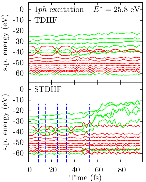
Figure 57: Time evolution of single particle energies in a TDHF calculation (upper panel) and in one STDHF event (lower panel) for an initial excitation energy of 25.8 eV. Red lines correspond to occupied states, green ones to unoccupied ones (see text for details). In the STDHF case, five $2ph$ transitions actually occurred (were actually sampled) for this event, transitions which are indicated by faint vertical dashed lines.

Each member of the ensemble will actually deliver a different sequence of transitions which will finally lead to the mixed state representing the correlated system. One can identify five $2ph$ transitions (indicated by faint dashed lines). It is also interesting to note that, up to minor mean field rearrangements, the TDHF evolution does preserve the arrangement of particle and hole states in the course of time evolution. Pure TDHF evolution more or less preserves initial occupations in time, hindering possible relaxation to a thermal state. STDHF overcomes overcomes this limitation as can be seen from the rearrangements in the lower panel.

Fig. 58 displays snapshots of occupation numbers, extracted from the one body density matrix, see Eq.(63), at several times along a STDHF propagation.

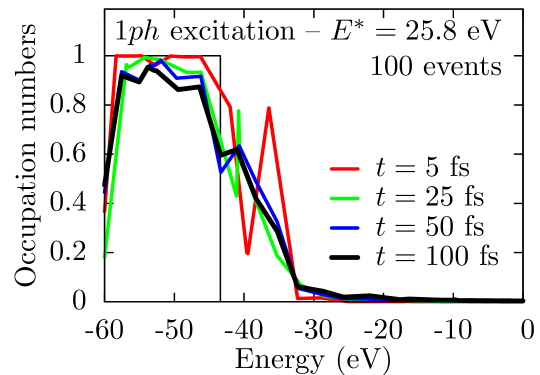
Figure 58: Snapshots of occupation numbers as a function of time in an example of STDHF calculation, with initial excitation $E^{*}$ of 25.8 eV and for a 100 event ensemble.

The occupation numbers keep for some time a trace of the original excitation, in particular the initial hole around $-37$ eV (see red curve). This hole is gradually filled and the occupation numbers are soon washed out, leading asymptotically to an energy profile typical of thermal equilibrium. Note some unavoidable statistical fluctuations, still visible at very low energy. This figure therefore demonstrates the capability of STDHF to account for relaxation effects at the side of electrons in a purely quantum mechanical manner. One should also stress that STDHF enables to estimate fluctuations around average values as computed from one or two-body density matrix, which again represents a remarkable step forward. The major obstacle of STDHF lies in the high cost of handling large ensembles which becomes particularly demanding for low excitation energies where smaller transition probabilities require better statistics. This still more development work is needed to put STDHF fully into action.

6 Conclusions

In this paper we have reviewed the analysis of electron emission following irradiation of clusters and molecules by light pulses. Observables from electron emission give detailed insight into the dynamical response of the irradiated species. Understanding the irradiation and emission process is also essential in view of the many applications in materials science, biology, and medicine. High-resolution studies of electron emission have made tremendous progress over the past few years, both experimentally and theoretically. In experiments, new developments in light sources now provide a broad choice of electromagnetic pulses with widely variable frequency, intensity, and time profile down to attosecond resolution in the range of electronic time scales. There is also great progress at the side of the measurement giving access to increasingly detailed properties of emitted electrons, high-resolution photo-electron spectra (PES) or angular distributions (PAD), often combined to velocity map imaging. As latest achievements, time-resolved PES/PAD are waiting in the wings. This remarkable experimental progress calls for elaborate theoretical treatments at the most microscopic level of description. In this respect, TDDFT, especially when solved in real time, constitutes an invaluable tool to simulate the various dynamical scenarios of irradiation of clusters and molecules. Therefore, many groups all over the world are heavily working on such approaches. In this review, we have presented a series of developments and results, mostly from the last decade, on irradiation of clusters and molecules by light pulses and subsequent detailed analysis of electron emission. Concerning the observables from emission, we consider total ionization, PES and PAD, also in connection with time-resolved measurements. At the theory side, we focus on a microscopic description in terms of time-dependent density functional theory (TDDFT). This is practically handled at the level of the time-dependent local density approximation (TDLDA) augmented by a self-interaction correction (SIC). We have illustrated the capabilities of our approach on several systems, ranging from simple molecules like N₂ to fashionable nano-clusters such as C₆₀, and also studying archetypal metal systems such as Na clusters. We list below a few results that we consider as being emblematic of these studies.

The theoretical modeling is based on TDDFT which is known to provide a robust microscopic description of the system dynamics. It enables to include ionic motion at a classical level. The fully coupled dynamics is needed in cases of long laser pulses and for thermal ensembles. In most cases, we consider short pulses and keep ions frozen. Starting level for TDDFT is the time-dependent local-density approximation (TDLDA). However, in order to describe ionization dynamics properly, one needs a theory fulfilling Koopmans’ theorem which states that the ionization potential (IP) has to be identical with the single particle (s.p.) energy of the least bound state. This is violated by the self-interaction error in LDA. It can be cured by augmenting LDA with a SIC. The latter has been turned manageable by a handling in terms of two sets of occupied s.p. states, the 2setSIC scheme. A less expensive alternative is offered by averaged density SIC (ADSIC) which performs surprisingly well as long as the dynamics stays off the regime of fragmentation and/or huge ionization. ADSIC has thus been used here in most cases and it allowed us to obtain remarkably accurate results in good agreement with experiments.

The numerical handling of ionization dynamics is most efficient in a coordinate-space representation. To describe ionization, we augment the coordinate-space grid by absorbing boundary conditions. They allow one to trivially compute the observables of total ionization and ionization out of each s.p. state separately (level depletion). PAD are computed by collecting the electron loss in angular segments on the grid. A complication arises when comparing PAD with measurements, since clusters or molecules in gas phase have an undefined orientation. They represent, in fact, an isotropic ensemble of orientations. Theoretical calculations need thus to be complemented by orientation averaging. For the one-photon domain, we have worked out a compact formula which can live with only six reference orientations to be computed. Multi-photon processes require direct integration where we find that one can obtain reliable results with typically 18–36 integration points, depending on the symmetry of the cluster. PES are computed by recording the phase oscillations of outgoing wave functions close to the onset of the absorbing bounds, and by finally Fourier transforming the temporal oscillations to the energy domain. Special care has to be taken to cope with strong laser pulses. They may modify the phase of the wave functions at the sampling point. Fortunately, this effect can be evaluated analytically and allows us to derive a phase correction, thus rendering the scheme for computing PES reliable up to rather large laser intensities (typically $10^{14}$–$10^{15}$W/cm². Altogether, we have thus at hand powerful and versatile tools to simulate ionization dynamics and to evaluate the observables deduced thereof. In the following, we will briefly summarize the results for each observable separately.

The simple signal of total ionization is already useful when combined with systematics. For example, the frequency dependence of ionization maps the underlying dipole response. Ionization becomes the key signal in pump and probe (P&P) scenarios which constitute a well established tool for a time-resolved measurement of ionic motion. Clusters are rather complex systems where the motion of single ions is hard to track. P&P measurements at least enable to identify global properties of the ionic configuration, as radius and quadrupole deformation, which is already very useful information in studies of Coulomb explosion of clusters. On a first example, we could show how the now upcoming attosecond pulses allow time-resolved analysis at electronic pace.

The main body of the paper dealt with results on PES and PAD. Combined PES/PAD as obtained from velocity map imaging (VMI) contain a very rich amount of information, but are usually hard to appreciate as such. The energy- or angular-integrated versions thereof, delivering PAD and PES, are better suited for detailed analysis and comparisons between experiments and theory. A PES in a strictly one-photon domain delivers a map of the clusters s.p. spectrum. In experiments, this was limited previously to negatively charge cluster anions due to a low ionization potential. The availability of coherent high-frequency light sources now allows one to employ the one-photon analysis for neutral clusters and even cations. Multi-photon processes make PES more involved and richer. In the low-intensity regime, one can identify multiple copies of the s.p. spectra separated by the photon frequency. But PES goes beyond just mapping s.p. spectra. It delivers a picture of the whole dynamical processes. We have illustrated that by working out the impact of plasmon resonances which can directly drop its signatures in the PES themselves. Increasing intensity produces more ionization which Coulomb shifts the s.p. states gradually downwards, thus broadening the peaks in the PES. This eventually leads to totally smoothed PES with straightforward exponential decrease. This kind of pattern suggests at first glance an interpretation as purely thermal electron emission. A closer inspection from energetic considerations and TDLDA simulations reveals that it cannot be fully a thermal process. We probably encounter a mixed situation. Direct emission still prevails and electronic re-collisions add first thermal effects to the picture. We have also seen that PES alone cannot distinguish unambiguously between direct and thermal emission.

The unavoidable orientation averaging of PAD wipes out many details which were contained in before averaging. Fortunately, there remains a lot of useful information. Orientation averaged PAD in the one-photon regime can be characterized by one single parameter, the anisotropy $\beta_{2}$. A systematic survey of $\beta_{2}$ and its frequency dependence revealed that PAD are extremely sensitive to every detail of the modeling. This holds even more so for state-resolved anisotropies $\beta_{2}^{(i)}$ (where $i$ stands for a s.p. state or degenerated group thereof). No compromises are allowed. One must invoke the full machinery of TDLDA+SIC and a careful description of the detailed ionic structure to have a chance for a relevant description. For example, the $\beta_{2}(\omega_{\rm las})$ computed with smooth jellium background shows marked fluctuations which disappear when ionic background is used. However, there remains one remarkable exception in the low-frequency tail of $\beta_{2}(\omega_{\rm las})$ for the loosely bound anion ${{\rm Na}_{7}}^{-}$. This shows a deep dip towards one-photon emission threshold and it does so independent of the model for the ionic background. In the multi-photon domain, a PAD provides crucial information which helps to distinguish direct from thermal emission. This was nicely visible in the combined PES/PAD of C₆₀ where one could associate uniquely the region of low kinetic energy with thermal electrons while higher kinetic energies show clear sign of direct emission with the PAD being forward/backward dominated.

The collection of results presented in this review has several open ends which call for further development and investigation. We briefly quote a few of them which we consider to be important next steps. It was already mentioned above that it becomes increasingly possible to extend time-resolved analysis to the attosecond domain. Theoretical studies are required to explore the huge space of new possibilities and to find out the most promising experimental conditions. A further interesting perspective emerges if combining time-resolved analysis with PES and PAD. This enables, e.g., to track the branching between direct and thermal emission in the course of time. First studies in this direction are very promising. The discussion of PES and PAD left as a yet unsolved problem the distinction between direct and thermal processes in electron emission. This calls for a proper theoretical modeling of electron-electron collisions (dynamical electron correlations) and subsequent dissipation effects. Two promising development lines for such an extended TDLDA have been presented, that is the relaxation time approach which models dissipation phenomenologically and a stochastic mean field model which describes the system as an ensemble of mean-field states incorporating the electron-electron collisions as stochastic jumps between these states.

The results summarized above prove that observables from electron emission are an extremely powerful tool to analyze irradiation processes on clusters and molecules. They allowed one in the past to reveal many interesting aspects of structure and dynamics of these systems. The future directions sketched in the previous paragraph show that we are not nearly at an end of the investigations. The field remains lively and highly interesting and challenging for the future.

References

- [1] U. Keller, Nature 424 (2003) 831.
- [2] C. Rullière (Ed.), Femtosecond Laser Pulses: Principles and Experiments, 2nd ed., Advanced Texts in Physics, Springer, New-York, 2005.
- [3] R. Paschotta, Encyclopedia of Laser Physics and Technology, volumes 1 and 2, Wiley-VCH, Berlin, 2008.
- [4] N. Ishikawa, Y. Saitoh, T. Yamaki, F. Hori, M. Sasase, Nucl. Inst. & Meth. B 314 (2013) 1.
- [5] G. Garcia, M. C. Fuchs, Series in Biological and Medical Physics, Biomedical Engineering, Springer-Verlag, Berlin, 2012.
- [6] Y. Zhang, Y. Wang, W. J. Weber, Nucl. Inst. & Meth. B, vol 286, 2012.
- [7] B. Liu, S. B. Nielsen, P. Hvelplund, H. Zettergren, H. Cederquist, B. Manil, B. A. Huber, Phys. Rev. Lett. 97 (2006) 133401.
- [8] G. Mie, Ann. Phys. (Leipzig) 25 (1908) 377.
- [9] U. Kreibig, M. Vollmer, Optical Properties of Metal Clusters, Vol. 25, Springer Series in Materials Science, 1993.
- [10] M. Brack, Rev. Mod. Phys. 65 (1993) 677.
- [11] W. A. de Heer, Rev. Mod. Phys. 65 (1993) 611.
- [12] P.-G. Reinhard, E. Suraud, Introduction to Cluster Dynamics, Wiley, New York, 2003.
- [13] U. Saalmann, C. Siedschlag, J. M. Rost, J. Phys. B 39.
- [14] F. Calvayrac, P.-G. Reinhard, E. Suraud, C. A. Ullrich, Phys. Rep. 337 (2000) 493.
- [15] T. Fennel, K.-H. Meiwes-Broer, J. Tiggesbäumker, P. M. Dinh, P.-G. Reinhard, E. Suraud, Rev. Mod. Phys. 82 (2010) 1793.
- [16] E. E. B. Campbell, K. Hansen, K. Hoffmann, G. Korn, M. Tchaplyguine, M. Wittmann, I. V. Hertel, Phys. Rev. Lett. 84 (2000) 2128.
- [17] C. Bartels, C. Hok, J. Huwer, R. Kuhnen, J. Schwöbel, B. von Issendorff, Science 323 (2009) 132333.
- [18] B. Boudaïffa, P. Cloutier, D. Hunting, M.-A. Huels, L. Sanche, Science 287 (2000) 1658.
- [19] I. Seideman, Ann. Rev. Phys. Chem. 53 (2002) 41.
- [20] M. Rohmer, M. Bauer, T. Leissner, C. Schneider, A. Fischer, G. Niedner-Schatteburg, B. von Issendorff, M. Aeschlimann, Phys. Status Solidi B 247 (2010) 1132.
- [21] M. A. L. Marques, N. T. Maitra, F. M. S. Nogueira, E. K. U. Gross, A. Rubio, Lect. Notes in Phys. vol 837, Springer-Verlag, Berlin, 2012.
- [22] T. Brabec, F. Krausz, Rev. Mod. Phys. 72 (2000) 545.
- [23] F. Krausz, M. Ivanov, Rev. Mod. Phys. 81 (2009) 163.
- [24] J. Feldhaus, J. Arthur, J. B. Hastings, J. Phys. B 38 (2005) 799.
- [25] L. V. Keldysh, Sov. Phys. JETP 20 (1964) 1307.
- [26] S. Augst, D. Strickland, D. D. Meyerhofer, S. L. Chin, J. H. Eberly, Phys. Rev. Lett. 63 (1989) 2212.
- [27] T. Seidemann, M. Y. Ivanov, P. B. Corkum, Phys. Rev. Lett. 75 (1995) 2819.
- [28] T. Zuo, A. D. Bandrauk, Phys. Rev. A 52 (1995) R2511.
- [29] V. Véniard, R. Taïeb, A. Maquet, Phys. Rev. A 65 (1) (2001) 013202.
- [30] C. Siedschlag, J. M. Rost, Phys. Rev. Lett. 89 (2002) 173401.
- [31] I. Last, J. Jortner, Phys. Rev. A 60 (1999) 2215.
- [32] H. Wabnitz, L. Bittner, A. R. B. de Castro, R. Dohrmann, P. Gurtler, T. Laarmann, W. Laasch, J. Schulz, A. Swiderski, K. von Haeften, T. Moller, B. Faatz, A. Fateev, J. Feldhaus, C. Gerth, U. Hahn, E. Saldin, E. Schneidmiller, K. Sytchev, K. Tiedtke, R. Treusch, M. Yurkov, Nature 420 (2002) 482.
- [33] L. Köller, M. Schumacher, J. Köhn, S. Teuber, J. Tiggesbäumker, K.-H. Meiwes-Broer, Phys. Rev. Lett. 82 (1999) 3783.
- [34] L. Schweikhard, A. Herlert, S. Krückeberg, M. Vogel, C. Walther, Phil. Mag. B 79 (1999) 1343.
- [35] T. Döppner, S. Teuber, M. Schumacher, J. Tiggesbäumker, K. Meiwes-Broer, Appl. Phys. B 71 (2000) 357.
- [36] E. Suraud, P.-G. Reinhard, Phys. Rev. Lett. 85 (2000) 2296.
- [37] U. Saalmann, J. M. Rost, Phys. Rev. Lett. 91 (2003) 223401.
- [38] T. Döppner, T. Fennel, T. Diederich, J. Tiggesbäumker, K. Meiwes-Broer, Phys. Rev. Lett. 94 (2005) 013401.
- [39] T. Döppner, T. Fennel, P. Radcliffe, J. Tiggesbäumker, K.-H. Meiwes-Broer, Phys. Rev. A 73 (2006) 031202.
- [40] C. Siedschlag, J. M. Rost, Phys. Rev. A 71 (2005) 031401(R).
- [41] T. Bornath, P. Hilse, M. Schlanges, Laser Phys. 17 (2007) 591.
- [42] S. Zamith, T. Martchenko, Y. Ni, S. A. Aseyev, H. G. Muller, M. J. J. Vrakking, Phys. Rev. A 70 (2004) 011201.
- [43] Y. L. Shao, T. Ditmire, J. W. G. Tisch, E. Springate, J. P. Marangos, M. H. R. Hutchinson, Phys. Rev. Lett. 77 (1996) 3343.
- [44] E. Springate, S. A. Aseyev, S. Zamith, M. J. J. Vrakking, Phys. Rev. A 68 (2003) 053201.
- [45] C. Bordas, F. Paulig, H. Heln, D. L. Huestis, Rev. Sci. Instr. 67 (1996) 2257.
- [46] O. Kostko, C. Bartels, J. Schwobel, C. Hock, B. v Issendorff, J. Phys. : Conf. Ser. 88 (2007) 012034.
- [47] M. Kjellberg, O. Johansson, F. Jonsson, A. V. Bulgakov, C. Bordas, E. E. B. Campbell, K. Hansen, Phys. Rev. A 81 (2010) 023202.
- [48] O. Cheshnovsky, K. J. Taylor, J. Conceicao, R. E. Smalley, Phys. Rev. Lett. 64 (1990) 1785.
- [49] G. Wrigge, M. A. Hoffmann, B. von Issendorff, Phys. Rev. A 65 (2002) 063201.
- [50] A. Pohl, P.-G. Reinhard, E. Suraud, J. Phys. B 37 (2004) 3301.
- [51] A. Rytkönen, H. Häkkinen, M. Manninen, Phys. Rev. Lett. 80 (1998) 3940.
- [52] K. Hansen, K. Hoffmann, E. E. B. Campbell, J. Chem. Phys. 119 (2003) 2513.
- [53] R. M. Young, M. A. Yandell, S. B. King, D. M. Neumark, J. Chem. Phys 136 (2012) 094304.
- [54] J. Wills, F. Pagliarulo, B. Baguenard, F. Lépine, C. Bordas, Chem. Phys. Lett. 390 (2004) 145.
- [55] Y. Yamaguchi, Y. Osamure, J. D. Goddard, H. Schaefer, A New Dimension to Quantum Chemistry: Analytic Derivative Methods in Ab Initio Molecular Electronic Structure Theory, Oxford University Press, Oxford, 1994.
- [56] P. Krause, T. Klamroth, P. Saalfrank, J. Chem. Phys. 127.
- [57] A. A. Vlasov, Many Particle Theory and Its Applications to Plasma, Gordon & Breach, New York, 1950.
- [58] G. F. Bertsch, S. Das Gupta, Phys. Rep. 160 (1988) 190.
- [59] A. Domps, E. Giglio, P.-G. Reinhard, E. Suraud, J. Phys. B 33 (2000) L333.
- [60] T. Fennel, G. F. Bertsch, K.-H. Meiwes-Broer, Eur. Phys. J. D 29 (2004) 367.
- [61] C. Sieber, W. Harbich, K.-H. Meiwes-Broer, C. Félix, Chem. Phys. Lett. 433 (2006) 32.
- [62] L. Szasz, Pseudopotential Theory of Atoms and Molecules, Wiley, New York, 1985.
- [63] S. Kümmel, M. Brack, P.-G. Reinhard, Eur. Phys. J. D 9 (1999) 149.
- [64] S. Goedecker, M. Teter, J. Hutter, Phys. Rev. B 54 (1996) 1703.
- [65] N. W. Ashcroft, N. D. Mermin, Solid State Physics, Saunders College, Philadelphia, 1976.
- [66] W. Ekardt, Z. Penzar, Phys. Rev. B 43 (1991) 1331.
- [67] B. Montag, T. Hirschmann, J. Meyer, P.-G. Reinhard, M. Brack, Phys. Rev. B 52 (1995) 4775.
- [68] P. Hohenberg, W. Kohn, Phys. Rev. 136 (1964) 864.
- [69] W. Kohn, L. J. Sham, Phys. Rev. 140 (1965) 1133.
- [70] R. G. Parr, W. Yang, Density-Functional Theory of Atoms and Molecules, Oxford University Press, Oxford, 1989.
- [71] R. M. Dreizler, E. K. U. Gross, Density Functional Theory: An Approach to the Quantum Many-Body Problem, Springer-Verlag, Berlin, 1990.
- [72] E. K. U. Gross, J. F. Dobson, M. Petersilka, Top. Curr. Chem. 181 (1996) 81.
- [73] A. D. Becke, Phys. Rev. A 38 (1988) 3098.
- [74] J. P. Perdew, K. Burke, M. Ernzerhof, Phys. Rev. Lett. 77 (1996) 3865.
- [75] J. P. Perdew, S. Kurth, A. Zupan, P. Blaha, Phys. Rev. Lett. 82 (1999) 2544.
- [76] A. K. Dhara, S. K. Ghosh, Phys. Rev. A 35 (1987) 442(R).
- [77] G. Vignale, W. Kohn, Phys. Rev. Lett. 77 (1996) 2037.
- [78] C. Ullrich, Oxford University Press, Oxford, 2012.
- [79] R. D’Agosta, G. Vignale, Phys. Rev. Lett. 96 (2006) 016405.
- [80] N. T. Maitra, I. Souza, K. Burke, Phys. Rev. B 68 (2003) 045109.
- [81] P. Bonche, B. Grammaticos, S. E. Koonin, Phys. Rev. C17 (1978) 1700.
- [82] J. Terasaki, P.-H. Heenen, H. Flocard, P. Bonche, Nucl. Phys. A 600 (1996) 371–386.
- [83] A. Castro, H. Appel, M. Oliveira, C. Rozzi, X. Andrade, F. Lorenzen, M. Marques, E. Gross, A. Rubio, Phys. Stat. Sol. B 243 (2006) 2465.
- [84] X. Andrade, J. Alberdi-Rodriguez, D. A. Strubbe, M. J. T. Oliveira, F. Nogueira, A. Castro, J. Muguerza, A. Arruabarrena, S. G. Louie, A. Aspuru-Guzik, A. Rubio, M. A. L. Marques, J. Phys.: Cond. Matt. 24 (2012) 233202.
- [85] R. Y. Cusson, R. K. Smith, J. A. Maruhn, Phys. Rev. Lett. 36 (1976) 1166–1169.
- [86] F. Calvayrac, P.-G. Reinhard, E. Suraud, Phys. Rev. B 52 (1995) R17056.
- [87] J. W. Eastwood, D. R. K. Brownrigg, J. Comp. Phys. 32 (1979) 24.
- [88] G. Lauritsch, P.-G. Reinhard, Int. J. Mod. Phys. C 5 (1994) 65.
- [89] P.-G. Reinhard, R. Y. Cusson, Nucl. Phys. A 378 (1982) 418.
- [90] M. D. Feit, J. A. Fleck, A. Steiger, J. Comp. Phys. 47 (1982) 412.
- [91] V. Blum, G. Lauritsch, J. A. Maruhn, P.-G. Reinhard, J. Comp. Phys 100 (1992) 364.
- [92] K. T. R. Davies, S. E. Koonin, Phys. Rev. C23 (1981) 2042–2061.
- [93] B. Montag, P.-G. Reinhard, Phys. Lett. A 193 (1994) 380.
- [94] T. Berkus, P.-G. Reinhard, E. Suraud, Int. J. Mol. Sci. 3 (2002) 69.
- [95] P. M. Dinh, F. Fehrer, P.-G. Reinhard, E. Suraud, Eur. Phys. J. D 45 (2007) 415.
- [96] P. M. Dinh, P.-G. Reinhard, E. Suraud, Phys. Rep. 485 (2010) 43.
- [97] R. S. Varga, Iterative Matrix Analysis, Prentice-Hall, Englewood Cliffs, 1962.
- [98] W. H. Press, S. A. Teukolsky, W. T. Vetterling, B. P. Flannery, Numerical Recipes, Cambridge University Press, Cambridge, 1992.
- [99] J. P. Perdew, A. Zunger, Phys. Rev. B 23 (1981) 5048.
- [100] J. Messud, P. M. Dinh, P.-G. Reinhard, E. Suraud, Ann. Phys. 324 (2009) 955.
- [101] M. R. Pederson, R. A. Heaton, C. C. Lin, J. Chem. Phys. 80 (5) (1984) 1972.
- [102] J. Messud, P. M. Dinh, P.-G. Reinhard, E. Suraud, Phys. Rev. Lett. 101 (2008) 096404.
- [103] S. Kümmel, L. Kronik, Rev. Mod. Phys. 80 (2008) 3.
- [104] J. B. Krieger, Y. Li, G. J. Iafrate, Phys. Rev. A 45 (1992) 101.
- [105] R. T. Sharp, G. K. Horton, Phys. Rev. 30 (1953) 317.
- [106] C. Legrand, E. Suraud, P.-G. Reinhard, J. Phys. B 35 (2002) 1115.
- [107] I. Ciofini, C. Adamo, H. Chermette, Chem. Phys. 309 (2005) 67–76.
- [108] P. Klüpfel, P. M. Dinh, P.-G. Reinhard, E. Suraud, Phys. Rev. A 88 (2013) 052501.
- [109] E. Fermi, E. Amaldi, Accad. Ital. Rome 6 (1934) 117.
- [110] Y. H. Yu, T. Zuo, A. D. Bandrauk, J. Phys. B 31 (1998) 1533.
- [111] U. De Giovannini, D. Varsano, M. A. L. Marques, H. Appel, E. K. U. Gross, A. Rubio, Phys. Rev. A 85 (2012) 062515.
- [112] K. Boucke, H. Schmitz, H.-J. Kull, Phys. Rev. A 56 (1997) 763.
- [113] M. Mangin-Brinet, J. Carbonell, C. Gignoux, Phys. Rev. A 57 (1998) 3245.
- [114] T. Nakatsukasa, K. Yabana, Phys. Rev. C 71 (2005) 024301.
- [115] J. L. Krause, K. J. Schafer, K. C. Kulander, Phys. Rev. A 45 (1992) 4998.
- [116] P.-G. Reinhard, E. Suraud, Cluster dynamics in strong laser fields, in: M. A. L. Marques, C. A. Ullrich, F. Nogueira (Eds.), Time-dependent density functional theory, Vol. 706 of Lecture Notes in Physics, Springer, Berlin, 2006, p. 391.
- [117] P.-G. Reinhard, P. D. Stevenson, D. Almehed, J. A. Maruhn, M. R. Strayer, Phys. Rev. E 73 (2006) 036709.
- [118] A. Pohl, P.-G. Reinhard, E. Suraud, Phys. Rev. A 70 (2004) 023202.
- [119] A. Pohl, P.-G. Reinhard, E. Suraud, Phys. Rev. Lett. 84 (2000) 5090.
- [120] A. Pohl, Ph.D. thesis, Friedrich-Alexander-Universität, Erlangen/Nürnberg (2003).
- [121] P. M. Dinh, P. Romaniello, P.-G. Reinhard, E. Suraud, Phys. Rev. A 87 (2013) 032514.
- [122] A. Gazibegovic-Busuladzic, E. Hasovic, M. Busuladzic, D. B. Milosevic, F. Kelkensberg, W. K. Siu, M. J. J. Vrakking, F. Lépine, G. Sansone, M. Nisoli, I. Znakovskaya, M. Kling, Phys. Rev. A 84 (2011) 043426.
- [123] D. B. Milošević, G. G. Paulus, D. Bauer, W. Becker, J. Phys. B 39 (14) (2006) R203.
- [124] H. Stapelfeldt, T. Seideman, Rev. Mod. Phys. 75 (2003) 543.
- [125] S. Pabst, R. Santra, Phys. Rev. A 81 (2010) 065401.
- [126] S. Pabst, R. Santra, Phys. Rev. A 82 (2010) 044901(E).
- [127] P.-G. Reinhard, E. Suraud, Eur. Phys. J. D 34 (2005) 145.
- [128] P. Wopperer, B. Faber, P. M. Dinh, P.-G. Reinhard, E. Suraud, Phys. Lett. A 375 (2010) 39.
- [129] P. Wopperer, B. Faber, P. M. Dinh, P.-G. Reinhard, E. Suraud, Phys. Rev. A 82 (2010) 063416.
- [130] A. R. Edmonds, Angular Momentum in Quantum Mechanics, Princeton University Press, Princeton, 1957.
- [131] K. Huang, Wiley, New York, 1963.
- [132] L. P. Kadanoff, G. Baym, Quantum Statistical Mechanics: Green’s Function Methods in Equilibrium and Nonequilibrium Problems, Frontiers in physics, Benjamin, New York, 1962.
- [133] R. Balescu, Equilibrium and Non-Equilibrium Statistical Mechanics, Wiley, New York, 1975.
- [134] E.-A. Uehling, G.-E. Uhlenbeck, Phys. Rev. 43 (1933) 552.
- [135] D. Durand, E. Suraud, B. Tamain, Nuclear Dynamics in the Nucleonic Regime, Institute of Physics, London, 2000.
- [136] A. Domps, P.-G. Reinhard, E. Suraud, Phys. Rev. Lett. 81 (1998) 5524.
- [137] A. Domps, P.-G. Reinhard, E. Suraud, Ann. Phys. (NY) 280 (2000) 211.
- [138] G. Chen, Oxford University Press, New York, 2005.
- [139] H. Uechi, Indiana University, Bloomington, 1988.
- [140] K. Husimi, Proc. Phys. Math. Soc. Jpn. 22 (1940) 264.
- [141] T. Körzdörfer, M. Mundt, S. Kümmel, Phys. Rev. Lett. 100 (13) (2008) 133004.
- [142] P.-G. Reinhard, E. Suraud, Ann. Phys. (NY) 239 (1995) 193.
- [143] A. T. J. B. Eppink, D. H. Parker, Rev. Sci. Instrum. 68 (1997) 3477.
- [144] M. Mundt, S. Kümmel, B. Huber, M. Moseler, Phys. Rev. B 73 (20) (2006) 205407.
- [145] T. Koopmans, Physica 1 (1934) 104.
- [146] P. M. Dinh, C. Z. Gao, P. Kluepfel, P.-G. Reinhard, E. Suraud, M. Vincendon, J. Wang, F. S. Zhang, submitted to Eur. J. Phys. D.
- [147] K. Yabana, G. F. Bertsch, Phys. Rev. B 54 (1996) 4484.
- [148] F. Calvayrac, P.-G. Reinhard, E. Suraud, Ann. Phys. (NY) 255 (1997) 125.
- [149] P.-G. Reinhard, S. Weisgerber, O. Genzken, M. Brack, Lecture Notes in Physics 404 (1992) 254.
- [150] P.-G. Reinhard, O. Genzken, M. Brack, Ann. Phys. (Leipzig) 5 (1996) 576.
- [151] M. Vincendon, P. M. Dinh, P. Romaniello, P.-G. Reinhard, E. Suraud, Eur. J. Phys. D 67 (2013) 97.
- [152] U. Ndongmouo-Taffoti, P. M. Dinh, P.-G. Reinhard, E. Suraud, Z. Wang, Eur. J. Phys. D 58 (2010) 131.
- [153] A. H. Zewail, Femtochemistry, Vol. I & II, World Scientific, Singapore, 1994.
- [154] B. M. Garraway, K.-A. Suominen, Rep. Prog. Phys. 58 (1995) 365.
- [155] T. Leisner, S. Vajda, S. Wolf, L. Wöste, J. Chem. Phys. 111 (1999) 1017.
- [156] R. Heinicke, J. Grotemeyer, Appl. Phys. B 71 (2000) 419.
- [157] M. Hartmann, J. Pittner, V. Bonacic-Koutecky, A. Heidenreich, J. Jortner, J. Chem. Phys. 108 (1998) 3096.
- [158] T. Döppner, J. P. Müller, A. Przystawik, J. Tiggesbäumker, K.-H. Meiwes-Broer, Eur. Phys. J. D 43 (2007) 261.
- [159] J.-H. Klein-Wiele, P. Simon, H.-G. Rubahn, Phys. Rev. Lett. 80 (1997) 45.
- [160] J.-H. Klein-Wiele, P. Simon, H.-G. Rubahn, Optics Comm. 161 (1999) 42.
- [161] M. Merschdorf, W. Pfeiffer, A. Thon, S. Voll, G. Gerber, App. Phys. A 71 (2000) 547.
- [162] M. Perner, S. Gresillon, J. März, G. von PLessen, J. Feldmann, J. Porstendorfer, K.-J. Berg, G. Berg, Phys. Rev. Lett. 85 (2000) 792.
- [163] G. Seifert, M. Kaempfe, K.-J. Berg, H. Graener, Appl. Phys. B 71 (2000) 795.
- [164] F. Stienkemeier, A. F. Vilesov, J. Chem. Phys. 115 (2001) 10119.
- [165] T. Döppner, T. Fennel, P. Radcliffe, J. Tiggesbäumker, K.-H. Meiwes-Broer, Eur. Phys. J. D 36 (2005) 165.
- [166] K. Andrae, P.-G. Reinhard, E. Suraud, J. Phys. B 35 (2002) 1.
- [167] K. Andrae, P.-G. Reinhard, E. Suraud, Phys. Rev. Lett. 92 (2004) 173402.
- [168] F. Calvayrac, E. Suraud, P.-G. Reinhard, J. Phys. B 31 (1998) 1367.
- [169] T. Fennel, T. Döppner, J. Passig, C. Schaal, J. Tiggesbäumker, K.-H. Meiwes-Broer, Phys. Rev. Lett. 98 (2007) 143401.
- [170] J. Passig, R. Irsig, N. Truong, T. Fennel, J. Tiggesbäumker, K.-H. Meiwes-Broer, New J. Phys. 14 (2012) 085020.
- [171] N. H. Damrauer, C. Dietl, G. Krampert, S.-H. Lee, K.-H. Jung, G. Gerber, Eur. Phys. J. D 20 (2002) 71.
- [172] V. Bonačić-Koutecký, R. Mitrić, T. Bernhardt, L. Wöste, J. Jortner, Adv. Phys. Chem. 132 (2005) 179.
- [173] N. Truong, P. Hilse, S. Göde, A. Przystawik, T. Döppner, T. Fennel, T. Bornath, J. Tiggesbäumker, M. Schlanges, G. Gerber, K.-H. Meiwes-Broer, Phys. Rev. A 81 (2010) 013201.
- [174] P. Johnsson, J. Mauritsson, T. Remetter, A. L’Huillier, K. J. Schafer, Phys. Rev. Lett. 99 (2007) 233001.
- [175] X. M. Tong, P. Ranitovic, C. L. Cocke, N. Toshima, Phys. Rev. A 81 (2010) 021404.
- [176] X.-M. Tong, N. Toshima, Phys. Rev. A 81 (2010) 043429.
- [177] M. Murakami, S.-I. Chu, Phys. Rev. A 88 (2013) 043428.
- [178] P. Rivière, O. Uhden, U. Saalmann, J. M. Rost, New J. Phys. 11 (2009) 053011.
- [179] G. Sansone, F. Kelkensberg, J. F. Pérez-Torres, F. Morales, M. F. Kling, W. Siu, O. Ghafur, P. Johnsson, M. Swoboda, E. Benedetti, F. Ferrari, F. Lépine, J. L. Sanz-Vicario, S. Zherebtsov, I. Znakovskaya, A. L’Huillier, M. Y. Ivanov, M. Nisoli, F. Martín, M. J. J. Vrakking, Nature 465 (2010) 763.
- [180] F. Kelkensberg, W. Siu, J. F. Pérez-Torres, F. Morales, G. Gademann, A. Rouzée, P. Johnsson, M. Lucchini, F. Calegari, J. L. Sanz-Vicario, F. Martín, M. J. J. Vrakking, Phys. Rev. Lett. 107 (2011) 043002.
- [181] W. Siu, F. Kelkensberg, G. Gademann, A. Rouzée, P. Johnsson, D. Dowek, M. Lucchini, F. Calegari, U. De Giovannini, A. Rubio, R. R. Lucchese, H. Kono, F. Lépine, M. J. J. Vrakking, Phys. Rev. A 84 (2011) 063412.
- [182] C. Neidel, J. Klei, C.-H. Yang, A. Rouzée, M. J. J. Vrakking, K. Klünder, M. Miranda, C. L. Arnold, T. Fordell, A. L’Huillier, M. Gisselbrecht, P. Johnsson, M. P. Dinh, E. Suraud, P.-G. Reinhard, V. Despré, M. A. L. Marques, F. Lépine, Phys. Rev. Lett. 111 (2013) 033001.
- [183] P. M. Paul, E. S. Toma, P. Breger, G. Mullot, F. Augé, P. Balcou, H. G. Muller, P. Agostini, Science 292 (5522) (2001) 1689–1692.
- [184] H. Muller, Applied Physics B 74 (1) (2002) s17.
- [185] M. Magrakvelidze, O. Herrwerth, Y. H. Jiang, A. Rudenko, M. Kurka, L. Foucar, K. U. Kühnel, M. Kübel, N. G. Johnson, C. D. Schröter, S. Düsterer, R. Treusch, M. Lezius, I. Ben-Itzhak, R. Moshammer, J. Ullrich, M. F. Kling, U. Thumm, Phys. Rev. A 86 (2012) 013415.
- [186] Y. H. Jiang, A. Senftleben, M. Kurka, A. Rudenko, L. Foucar, O. Herrwerth, M. F. Kling, M. Lezius, J. V. Tilborg, A. Belkacem, K. Ueda, D. Rolles, R. Treusch, Y. Z. Zhang, Y. F. Liu, C. D. Schröter, J. Ullrich, R. Moshammer, J. Phys. B 46 (16) (2013) 164027.
- [187] P. Tzallas, E. Skantzakis, L. A. A. Nikolopoulos, G. D. Tsakiris, D. Charalambidis, Nat. Phys. 7 (2011) 781.
- [188] P. A. Carpeggiani, P. Tzallas, A. Palacios, D. Gray, F. Martín, D. Charalambidis, Phys. Rev. A 89 (2014) 023420.
- [189] A. Palacios, A. González-Castrillo, F. Martín, Proc. Nat. Acad. Sci. 111 (11) (2014) 3973.
- [190] P. Wopperer, Ph.D. thesis, Université Paul Sabatier (2013).
- [191] P. Wopperer, C. Z. Gao, T. Barillot, C. C. amd A Marciniak, V. Despré, V. Loriot, G. Celep, C. Bordas, F. Lépine, P. M. Dinh, E. Suraud, P.-G. Reinhard, submitted to Phys. Rev. Lett.
- [192] P. M. Dinh, S. Vidal, P.-G. Reinhard, E. Suraud, New J. Phys. 14 (2012) 063015.
- [193] A. Pohl, P.-G. Reinhard, E. Suraud, J. Phys. B 34 (2001) 4969.
- [194] P. Wopperer, P. M. Dinh, P.-G. Reinhard, E. Suraud, J. Phys.: Conf. Series 438 (2013) 95.
- [195] H. Bethe, Handbuch der Physik, Band 24/1, Springer, Berlin, 1933.
- [196] J. Cooper, R. N. Zare, J. Chem. Phys. 48 (1968) 942.
- [197] J. Cooper, R. N. Zare, J. Chem. Phys. 49 (1968) 4252.
- [198] E. Maurat, P. A. Hervieux, F. Lépine, J. Phys. B 42 (2009) 165105.
- [199] J. Cooper, R. N. Zare, Photoelectron Angular Distributions, Gordon and Breach, New York, 1969.
- [200] A. D. Buckingham, B. J. Orr, J. M. Sichel, Philos. Trans. Royal Soc. London, Series A 268 (1970) 147.
- [201] L. I. Schiff, McGraw-Hill, New York, 1968.
- [202] P. Wopperer, P. M. Dinh, E. Suraud, P.-G. Reinhard, Phys. Rev. A 85 (2012) 015402.
- [203] C. Bartels, Ph.D. thesis, Albert-Ludwigs-Universität Freiburg (2008).
- [204] A. V. Solov’yov, R. G. Polozkov, V. K. Ivanov, Phys. Rev. A 81 (2010) 021202(R).
- [205] T. Barillot, C. Cauchy, P.-A. Hervieux, M. Gisselbrecht, S. E. Canton, P. Johnsson, J. Laksman, E. P. Mansson, J. M. Dahlström, E. Suraud, P. Dinh, P. Wopperer, K. Hansen, V. Loriot, C. Bordas, S. Sorensen, F. Lépine, submitted to Phys. Rev. Lett.
- [206] L. Schweikhard, S. Krückeberg, K. Lützenkirchen, C. Walther, Eur. Phys. J. D 9 (1999) 15.
- [207] H. Haberland, T. Hippler, J. Donges, O. Kostko, M. Schmidt, B. von Issendorff, Phys. Rev. Lett. 94 (2005) 035701.
- [208] R. Schlipper, R. Kusche, B. von Issendorff, H. Haberland, Appl. Phys. A 72 (2001) 255.
- [209] E. Giglio, P.-G. Reinhard, E. Suraud, Ann. Phys. (Leipzig) 11 (2002) 291.
- [210] E. Giglio, P.-G. Reinhard, E. Suraud, Phys. Rev. A 67 (2003) 43202.
- [211] E. Giglio, P.-G. Reinhard, E. Suraud, J. Phys. B 34 (2001) 1253.
- [212] P.-G. Reinhard, E. Suraud, Eur. Phys. J. D 3 (1998) 175.
- [213] J. A. R. Samson, R. B. Cairns, J. Opt. Soc. Am. 55 (1965) 1035.
- [214] H. D. Cohen, U. Fano, Phys. Rev. 150 (1966) 30–33.
- [215] F. Frémont, A. Hajaji, A. Naja, C. Leclercq, J. Soret, J. A. Tanis, B. Sulik, J.-Y. Chesnel, Phys. Rev. A 72 (2005) 050704.
- [216] S. Chatterjee, D. Misra, A. H. Kelkar, L. C. Tribedi, C. R. Stia, O. A. Fojón, R. D. Rivarola, Phys. Rev. A 78 (2008) 052701.
- [217] S. Chatterjee, A. N. Agnihotri, C. R. Stia, O. A. Fojón, R. D. Rivarola, L. C. Tribedi, Phys. Rev. A 82 (2010) 052709.
- [218] J. L. Baran, S. Das, F. Járai-Szabó, K. Póra, L. Nagy, J. A. Tanis, Phys. Rev. A 78 (2008) 012710.
- [219] S. Nandi, A. N. Agnihotri, S. Kasthurirangan, A. Kumar, C. A. Tachino, R. D. Rivarola, F. Martí n, L. C. Tribedi, Phys. Rev. A 85 (2012) 062705.
- [220] M. Winkworth, P. Fainstein, M. Galassi, J. Baran, B. Dassanayake, S. Das, A. Kayani, J. Tanis, Nucl. Instr. Meth. Phys. Res. B 267 (2) (2009) 373, proceedings of the Fourth International Conference on Elementary Processes in Atomic Systems.
- [221] A. N. Agnihotri, S. Nandi, S. Kasthurirangan, A. Kumar, M. E. Galassi, R. D. Rivarola, C. Champion, L. C. Tribedi, Phys. Rev. A 87 (2013) 032716.
- [222] S. Nandi, S. Biswas, A. Khan, J. M. Monti, C. A. Tachino, R. D. Rivarola, D. Misra, L. C. Tribedi, Phys. Rev. A 87 (2013) 052710.
- [223] M. Bär and B. Jakob and P.–G. Reinhard and C. Toepffer, Phys. Rev. A 73 (2006) 022719.
- [224] K. Goeke, P.-G. Reinhard, H. Reinhardt, Ann. Phys. 166 (1986) 257.
- [225] Y. Abe, S. Ayik, P.-G. Reinhard, E. Suraud, Phys. Rep. 275 (1996) 49.
- [226] C. Wong, K. Davies, Phys. Rev. C 28 (1983) 2321.
- [227] R. Cusson, P.-G. Reinhard, J. Maruhn, W. Greiner, M. Strayer, Z. Phys. A 320 (1985) 475.
- [228] A. Umar, V. Oberacker, Phys. Rev. C 74 (2006) 021601R.
- [229] G. Bertsch, Z. Phys. A 289 (1978) 103.
- [230] P. Danielewicz, Phys. Lett. B 146 (1984) 168.
- [231] P. Danielewicz, Ann. Phys. (N.Y.) 152 (1984) 239.
- [232] P. Danielewicz, Ann. Phys. (N.Y.) 152 (1984) 305.
- [233] J. Lehmann, M. Merschdorf, W. Pfeiffer, A. Thon, S. Voll, G. Gerber, Phys. Rev. Lett. 85 (2000) 2921.
- [234] P.-G. Reinhard, E. Suraud, Ann. Phys. (NY) 216 (1992) 98.
- [235] M. Bixon, R. Zwanzig, Phys. Rev. 187 (1969) 267.
- [236] R. Zwanzig, J. Stat. Phys. 9 (1973) 215.
- [237] S. Ayik, C. Gregoire, Phys. Lett. B 212 (1988) 269.
- [238] J. Randrup, G. F. Burgio, P. Chomaz, Nucl. Phys. A 538 (1992) 393.
- [239] P. Napolitani, M. Colonna, Phys. Lett. B 726 (2013) 382.
- [240] N. Slama, P. M. Dinh, P. G. Reinhard, E. Suraud, J. Phys. Conf. Ser., in press.
- [241] L. van Hove, Physica 21 (1955) 517.