Boiling of the Interface between Two Immiscible Liquids below the Bulk Boiling Temperatures of Both Components

Abstract

We consider the problem of boiling of the direct contact of two immiscible liquids. An intense vapour formation at such a direct contact is possible below the bulk boiling points of both components, meaning an effective decrease of the boiling temperature of the system. Although the phenomenon is known in science and widely employed in technology, the direct contact boiling process was thoroughly studied (both experimentally and theoretically) only for the case where one of liquids is becoming heated above its bulk boiling point. On the contrary, we address the case where both liquids remain below their bulk boiling points. In this paper we construct the theoretical description of the boiling process and discuss the actualisation of the case we consider for real systems.

1 Introduction

The process of boiling of a system of two immiscible liquids has a remarkable feature: it can occur at temperatures below the bulk boiling temperatures of both components (e.g., see Krell-1982 ; Geankoplis-2003 ). This phenomenon is explained by the fact that boiling occurs at the interface between two liquids, but not in their bulk. Molecules from both liquids evaporate into the vapour layer between two liquids and each liquid tends to be in local thermodynamic equilibrium with its vapour, therefore equilibrium pressure within this layer is equal to the sum of the saturated vapour pressures of both liquids. Hence, the condition for the growth of the vapour phase is the exceeding of atmospheric pressure by the sum of the saturated vapour pressures, while for the bulk boiling the vapour pressure alone should exceed atmospheric pressure.

The phenomenon under consideration is widely used in industry Krell-1982 ; Geankoplis-2003 . For instance, it is beneficial for distillation of substances the boiling temperature of which is higher than the decomposition temperature at atmospheric pressure (as it is for insoluble tetraethyllead). This phenomenon is employed for combustion of poorly volatile liquid fuels in furnaces. Simultaneously, it is the reason why water is forbidden for usage when one needs to stop fire of inflammable organic liquids. The phenomenon is also of interest in relation to the process of combustion of a light inflammable liquid covering the surface of a heavy nonflammable liquid.

Although this phenomenon is well known in the literature, many experimental Simpson-etal-1974 ; Celata-1995 ; Roesle-Kulacki-2012-1 ; Roesle-Kulacki-2012-2 and theoretical works Sideman-Isenberg-1967 ; Kendoush-2004 deal with the case where one of components is heated above its bulk boiling temperature. The case of interfacial boiling below the bulk boiling temperatures of both components did not receive a thorough study in the literature. Meanwhile, this case is most intriguing as the one where boiling becomes possible being impossible otherwise. Moreover, there are situations in real systems, where exactly this case becomes relevant (see Sec. 2).

The interfacial boiling starts at temperature $T_{\ast}$ determined by the condition that the consolidated pressure of the saturated vapours of both liquids is equal to atmospheric pressure. In terms of the particle number densities $n_{j}^{(0)}$ of saturated vapours:

$$n_{1}^{(0)}(T_{\ast})+n_{1}^{(0)}(T_{\ast})=\frac{p_{0}}{k_{\mathrm{B}}T_{\ast}}\,,$$

where $p_{0}$ is atmospheric pressure, $k_{\mathrm{B}}$ is the Boltzmann constant. We will consider the case where both components are below their bulk boiling points, i.e., the temperature field in the system does not exceed $T_{\ast}$ significantly. In this case, vapour is generated only at the direct contact of two liquid; a growing vapour layer forms in between the liquids and experiences “resetting” to zero thickness from time to time because of vapour breakaway.

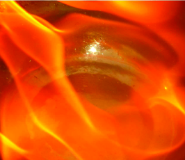
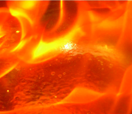
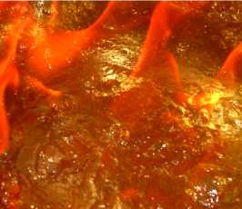
(a)	(b)	(c)

Figure 1: Demonstration experiment: Combustion of layer of “white spirit” (light fractions of kerosine) over water. (a): Nearly immediately after ignition, the flammable liquid and water are stably stratified (convective flows are suppressed); there is only intense surface evaporation of burning liquid, no bulk boiling. This regime is the regime of combustion as it would occur without underlying liquid. (b): $2\,\mathrm{min}$ after ignition, one can see rare vapour bubbles rising from the white spirit–water interface. The bulk boiling of water does not occur, meaning the interface temperature is below the bulk boiling points of both liquids. Intensity of interface boiling increases over time as white spirit layer becomes thinner and the heat influx to the interface increases. (c): $4\,\mathrm{min}$ after ignition, boiling of the interface is intense, although a stratified state persists in some form. Demonstration experiment set-up: The two-layer system was placed in a steel cavity of internal diameter $16\,\mathrm{cm}$; the initial thicknesses of white spirit and water layers: $2\,\mathrm{cm}$ and $3\,\mathrm{cm}$, respectively; air temperature and initial temperature of white spirit: $20^{\circ}\mathrm{C}$, initial water temperature: $40^{\circ}\mathrm{C}$. Timing for the combustion process significantly varies depending on air temperature and wind strength.

For methodological reasons, the particular case of two liquids with nearly identical values of physical chemical parameters was addressed as a first step of theoretical study of the phenomenon Pimenova-Goldobin-JETP-2014 . In this paper we extend the consideration to the case of different quantitative characteristics of liquids and also allow for the asymmetry between states of two liquids (which is important even when their properties are similar). Additionally, the demonstration experiments with combustion of a light inflammable liquid layer over a heavy nonflammable one are described and an auxiliary problem of the hydrodynamic instability of a thin vapour layer between heavy and light liquids to bubble formation is investigated in the Appendix.

The paper is organised as follows. In Sec. 2, the process of combustion of a light inflammable liquid over a heavy nonflammable one is discussed. In Sec. 3, we formulate the specific physical problem we deal with and derive the mathematical model of the system from scratch. In Sec. 4 we derive the solution to the mathematical model, which describes the growth of the vapour layer. In Sec. 5, relationships between macroscopic quantifiers of the system state and the derived growing-vapour-layer solution are established; the problem of the vapour bubble formation and the associated vapour layer breakaway is addressed for the cases of a well-stirred system and a stratified one. In Sec. 6, we overview the simplification assumptions of our work and perform quantitative assessments related to their accuracy. In Sec. 7, we draw conclusions. Solutions to several auxiliary problems are provided in Appendices.

(a)

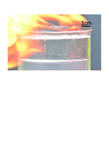
(b)

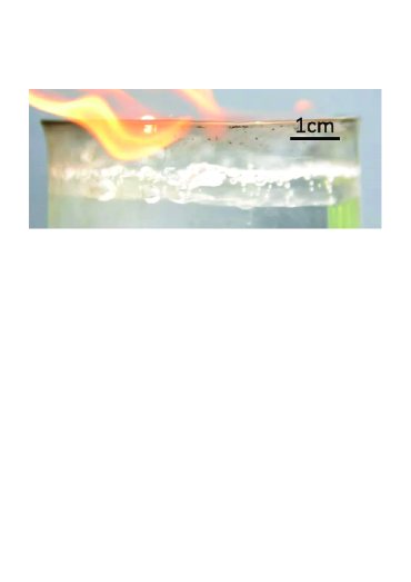
Figure 2: Demonstration experiment: Combustion of layer of n-heptane over water. (a) Early stage of boiling of the h-heptane–water interface: one centre of vapour formation and a bubble lane from it can be observed. (b): Intense boiling at the interface: a plenty of bubble lanes running from the interface can be observed, nearly all of them are away from the glass wall. Demonstration experiment set-up: The two-layer system was placed in a quartz glass of diameter $7\,\mathrm{cm}$; air temperature and initial temperature of n-heptane: $20^{\circ}\mathrm{C}$, initial water temperature: $90^{\circ}\mathrm{C}$.

2 Example: Combustion of light inflammable liquid over heavy nonflammable one

Prior to constructing the phenomenon theory, we would like to substantiate our interest to the specific case we consider not only by the reason of academic curiosity and non-triviality of the phenomenon of the decrease of the boiling point but also by practical reasons. We intend to discuss the primary relevance of specifically the case under consideration for combustion of a light inflammable liquid over a heavy nonflammable one.

Necessity of this argumentation is dictated by the fact that previously only the case of superheating conditions for one of components was addressed in experimental studies. This choice for experiment setups was related to industrial applications. However, we are to explain that this is not the only case which can be of practical importance. Obviously, even for the case, where one of components to be mainly superheated, the system unavoidably passes through the transient regimes where interfacial boiling still or already occurs but both components are not superheated. These can be late stages of self-cooling of the system without heat supply or early stages of mixing of two liquids, temperatures of which are such that one of liquids will be superheated before the system reaches thermal equilibrium. However, there are situations where the system is maintaining itself in the regime of our interest, the regime persists but not occur as a stage of a transient process. For these situations the relevance of our work is more pronounced.

Let us consider combustion of a light inflammable liquid over a heavy nonflammable one. We need first to remind that combustion of an inflammable liquid in an open container happens without the bulk boiling: there is only an intense surface evaporation. Indeed, the burning surface is heated to the bulk boiling temperature and the bulk of liquid is at lower temperature. If the heat influx from the flame becomes strong enough to heat the bulk above the boiling point, intense vapour formation starts. Given not enough oxygen (which is accessible only outside the liquid) provided, the vapour combustion area (flame) will be pushed away from the liquid by an intense vapour flux and thus liquid heating efficiency will be decreased.[] Noteworthy, in the course of such a combustion the liquid is stably stratified due to temperature gradient and all convective currents are suppressed Incropera-etal-2006 . The presence of another liquid below the burning one can change the situation. The interface between these two liquids can be heated to the interfacial boiling temperature without exceeding the bulk boiling temperature within the burning liquid. Boiling of this interface may have different effects on the combustion process, depending on the physical properties of liquids and system configuration. However, it is certain, that the interfacial boiling will be maintained at conditions we are to consider. Moreover, if the inflammable liquid is more volatile than the heavier bottom liquid (for instance, n-heptane over water), both components will be never superheated.

We performed demonstration experiments with “white spirit”–water (Fig. 1) and n-heptane–water (Fig. 2) systems. With these demonstration experiments (see Figs. 1, 2 and video in supplementary material or on YouTube YouTube ) one can observe the interfacial boiling in the course of combustion of organic fuel. The effect of this interfacial boiling on the combustion process will be considered elsewhere in detail; here we provide this example in support of physical and practical relevance of the problem set-up we will be using.

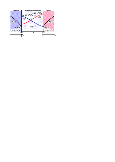
Figure 3: Growing vapour layer between two half-spaces of immiscible liquids and the reference frames.

3 Evolution of the vapour layer

The mathematical description of the dynamics of the system (Fig. 3) is based on the following physical assumptions:

1. Temperature in the zones of the liquid phases is nonuniform in order to provide the heat inflow to the surface of the evaporation.

2. The mass of the liquid phase decreases in the course of evaporation and the surfaces move deeper into liquids.

3. The substances evaporate from the surfaces of liquids into the vapour layer. We consider liquids which are mutually insoluble; therefore, the molecules of the first substance do not pass into the liquid phase at the second liquid–vapour interface. Immediately above the liquid surface, the number density $n_{j}$ ($j=1,2$) of the particles of the corresponding substance is equal to the particle number density of the saturated vapour, say $n_{j}^{(0)}$, of this substance at local temperature $T$

   $$n_{2}(z=-L_{2})=n_{2}^{(0)}(T),\quad n_{1}(z=L_{1})=n_{1}^{(0)}(T).$$

   When the liquid evaporate from free surface (e.g. into vacuum), the number density of the vapour above the surface is lower than the one of the saturated vapour due to finite escape rate of the evaporant and rapid diffusion outflow of particles from the surface Anisimov-Rakhmatulina-1973 . In the system under consideration, liquids evaporate not into the open half-space, but into the vapour layer. The differences of the number densities across the layer tend to zero for $T\to T_{\ast}$, and the diffusion outflow becomes asymptotically small, making the transition rates between the vapour and liquid phases sufficient to maintain the local thermodynamic equilibrium between the phases. Thus, the assumption of the local thermodynamic equilibrium at the vapour-liquid interface can be considered to be valid by continuity as long as the overheating of the system is small enough.

4. Pressure within the vapour layer is assumed to be constant and equal to atmospheric pressure, $p=p_{0}$, due to the negligibility of the mechanical inertia compared to the heat and diffusion “inertia” of the system.

5. The total number density of particles in the vapour layer obeys the ideal gas law

   $$n_{1}+n_{2}=n_{0}=\frac{p_{0}}{k_{B}T}\,,$$

   where $T$ is local temperature. The variation of $n_{0}$ associated with the temperature deviation from $T_{\ast}$ is negligible compared to the variation of $n_{j}$; thus,

   $$n_{1}+n_{2}=n_{0\ast}=\frac{p_{0}}{k_{B}T_{\ast}}\,.$$ (1)

For the interfacial boiling to occur the system must be overheated above the minimal temperature of boiling $T_{\ast}$:

$$T=T_{\ast}+\Theta\,,\qquad\Theta>0\,.$$

We focus our consideration on the case where both liquids are far from boiling conditions in their bulk, as the most intriguing one from the research view point. For the vapour layer, where heat is consumed for evaporation, the temperature excess above $T_{\ast}$ is even smaller than for the bulk. Hence, one can linearise the dependence of the saturated vapour number density $n_{j}^{(0)}(T)$ about $T=T_{\ast}$;

$$n_{j}^{(0)}(T_{\ast}+\Theta)=n_{j\ast}^{(0)}+\gamma_{j}\Theta+\dots\,,$$ (2)

where $n_{j\ast}^{(0)}\equiv n_{j}^{(0)}(T_{\ast})$ and $\gamma_{j}\equiv(\partial n_{j}^{(0)}/\partial T)_{T=T_{\ast}}$.

We deal with temperature variations which are small compared to the absolute temperature, $\delta T/T\ll 1$; therefore, for physical parameters which depend on temperature polynomially one can neglect variations due to their smallness (e.g., $n_{0}\propto 1/T$ and $|\delta n_{0}|/n_{0}=|\delta T|/T\ll 1$). On the contrary, for parameters which are exponential in $T$ one has to take this dependence into account. E.g., for the number density of saturated vapour $n^{(0)}(T)/n^{(0)}(T_{\ast})\propto e^{(T-T_{\ast})/T_{0}}$, where $T_{0}$ is of the order of magnitude of $10\,\mathrm{K}$, and $|\delta n^{(0)}|/n^{(0)}=|\delta T|/T_{0}$, which is by factor 30–40 larger than $|\delta T|/T$. We will construct our theory for small but non-negligible terms $\sim|\delta T|/T_{0}$ and neglect contributions $\sim|\delta T|/T$.

It is convenient to use different reference frames for three areas: for the liquids 1 and 2 the coordinates $z_{1}$ and $z_{2}$ measure shifts from the respective liquid surfaces and for the vapour layer the coordinate $z$ is in the range from $-L_{2}$ to $L_{1}$ (see Fig. 3).

Let us first consider the molecule number balance in the system. The number density redistribution of species within the vapour layer is due to molecular diffusion governed by the Fick’s law

$$\vec{J}_{j}=-D_{12}\nabla n_{j},$$ (3)

where $D_{12}$ is the coefficient of mutual diffusion. The dependence of this coefficient on temperature is a power law and, therefore, can be neglected as discussed above. Thus, the evolution of the number densities is governed by

$$\frac{\partial n_{j}}{\partial t}=\nabla\cdot(D_{12}\nabla n_{j})=D_{12}\frac{\partial^{2}n_{j}}{\partial z^{2}}\,.$$ (4)

For the boundary conditions on the number densities, we employ linearised dependencies $n_{j}^{(0)}(T)$, Eq. (2);

$$n_{1}|_{z=L_{1}} =n_{1*}^{(0)}+\gamma_{1}\Theta\,,$$ (5)

$$n_{2}|_{z=-L_{2}} =n_{2*}^{(0)}+\gamma_{2}\Theta\,.$$ (6)

Due to Eq. (1), Eqs. (5)–(6) yield as well

$$n_{2}|_{z=L_{1}} =n_{2*}^{(0)}-\gamma_{1}\Theta\,,$$ (7)

$$n_{1}|_{z=-L_{2}} =n_{1*}^{(0)}-\gamma_{2}\Theta\,.$$ (8)

The condition of molecule flux balance on the liquid–vapour interfaces is to be accounted as well. This condition yields the vapour layer growth rate. The variation of the number of molecules of one specie above the surface of the other specie liquid is driven by diffusion only. Thus, if there is an increase of the vapour layer thickness by $\delta{L_{2}}$ owned by evaporation from the liquid 2 in time interval $\delta{t}$, the molecules of specie 1 can populate this added layer $\delta{L_{2}}$ only due to diffusive influx from the bulk of the vapour layer in the same time interval $\delta{t}$, which mathematically reads

$$\left.n_{1}\right|_{z=-L_{2}}\delta L_{2} =D_{12}\left.\frac{\partial n_{1}}{\partial z}\right|_{z=-L_{2}}\delta t\,,$$

$$\left.n_{2}\right|_{z=L_{1}}\delta L_{1} =-D_{12}\left.\frac{\partial n_{2}}{\partial z}\right|_{z=L_{1}}\delta t\,.$$

These equalities yield

$$\dot{L}_{2} =\frac{D_{12}}{\left.n_{1}\right|_{z=-L_{2}}}\left.\frac{\partial n_{1}}{\partial z}\right|_{z=-L_{2}}\approx\frac{D_{12}}{n_{1\ast}^{(0)}}\left.\frac{\partial n_{1}}{\partial z}\right|_{z=-L_{2}},$$ (9)

$$\dot{L}_{1} =-\frac{D_{12}}{\left.n_{2}\right|_{z=L_{1}}}\left.\frac{\partial n_{2}}{\partial z}\right|_{z=L_{1}}\approx-\frac{D_{12}}{n_{2\ast}^{(0)}}\left.\frac{\partial n_{2}}{\partial z}\right|_{z=L_{1}},$$ (10)

where the dot symbol denotes the time-derivative; for the approximate equalities, we neglected relative corrections of order $\delta n_{j}^{(0)}/n_{j}^{(0)}$ which do not affect the leading order of accuracy. For the total thickness $L=L_{1}+L_{2}$,

$$\dot{L}=D_{12}\left(\frac{1}{n_{1\ast}^{(0)}}\left.\frac{\partial n_{1}}{\partial z}\right|_{z=-L_{2}}-\frac{1}{n_{2\ast}^{(0)}}\left.\frac{\partial n_{2}}{\partial z}\right|_{z=L_{1}}\right).$$ (11)

It is convenient to introduce quantifiers for the liquid phase evaporation rate. Let $v_{lj}$ be the velocity of the $j$-th liquid in the reference frame fixed to its surface ($v_{l1}<0$, $v_{l2}>0$); in other terms, $|v_{lj}|$ is the speed of the liquid phase retreat owned by evaporation. This velocity to be calculated from the particle conservation condition as follows. Let us consider the retreat of the surface of liquid 2 for $v_{l2}\delta t$ owned by evaporation of the molecules into the vapour layer. The number of molecules evaporated from the area $S$, $n_{l2}\cdot S\cdot(v_{l2}\delta t)$ (where $n_{l2}$ is the number density in the 2nd liquid phase) partially fills the newly-formed “slice” $\delta L_{2}$ of the vapour layer with particles of sort 2 and partially diffusively outflows from this slice downhill the number density gradient, deeper into the vapour layer;

$$n_{l2}Sv_{l2}\delta t=\left.n_{2}^{(0)}\right|_{z=-L_{2}}S\delta L_{2}-D_{12}\left.\frac{\partial n_{2}}{\partial z}\right|_{z=-L_{2}}S\delta t\,.$$

Since $dn_{2}=-dn_{1}$ (see Eq. (1)), the number density gradient at $z=-L_{2}$ can be taken from Eq. (9) and the latter equation yields (to the leading order of accuracy)

$$v_{l2}\approx\frac{n_{0*}}{n_{l2}}\dot{L}_{2}\,;$$ (12)

similarly,

$$v_{l1}\approx-\frac{n_{0*}}{n_{l1}}\dot{L}_{1}$$ (13)

(here, recall, $n_{lj}$ is the molecule number density in the $j$-th liquid phase).

Let us now consider the energy balance in the system. The total heat $Q_{S}$ supplied from the bulk of two liquids to the boiling interface per its unit area,

$$\dot{Q}_{S}=\kappa_{1}\left.\frac{\partial T_{1}}{\partial z_{1}}\right|_{z_{1}=0}-\left.\kappa_{2}\frac{\partial T_{2}}{\partial z_{2}}\right|_{z_{2}=0}$$ (14)

(here $\kappa_{i}$ is the heat conductivity coefficient), is consumed for evaporation from the liquid surfaces;

$$\dot{Q}_{S}=\Lambda_{1}n_{l1}(-v_{l1})+\Lambda_{2}n_{l2}v_{l2}\,,$$ (15)

where $\Lambda_{j}$ is the enthalpy of vaporization per one molecule. In order to describe the difference between heat influxes from the bulk of two liquids, one needs an additional quantifier

$$\dot{q}_{S}=\kappa_{1}\left.\frac{\partial T_{1}}{\partial z_{1}}\right|_{z_{1}=0}-\Bigg{(}-\left.\kappa_{2}\frac{\partial T_{2}}{\partial z_{2}}\right|_{z_{2}=0}\Bigg{)}.$$

Then, one can define the temperature boundary conditions for the system;

$$\left.\frac{\partial T_{1}}{\partial z_{1}}\right|_{z_{1}=0} =+\frac{1}{2\kappa_{1}}\left(\dot{Q}_{S}+\dot{q}_{S}\right),$$ (16)

$$\left.\frac{\partial T_{2}}{\partial z_{2}}\right|_{z_{2}=0} =-\frac{1}{2\kappa_{2}}\left(\dot{Q}_{S}-\dot{q}_{S}\right).$$ (17)

The heat conduction in the liquid phases is described by the equation

$$\frac{\partial T_{j}}{\partial t}+v_{lj}\frac{\partial T_{j}}{\partial z_{j}}=\chi_{j}\frac{\partial^{2}T_{j}}{\partial z_{j}^{2}}\,,$$ (18)

where $\chi_{j}$ is the temperature diffusivity coefficient.

The evolution of the vapour layer is completely specified by Eqs. (3) and (18) with the boundary conditions (5)–(8) and (16), (17), where $\dot{L}$ is given by Eq. (11), $v_{lj}$ are given by Eqs. (12) and (13), $\dot{Q}_{S}$ is given by Eq. (15).

4 Solution to the equations of the vapour layer evolution

According to the results derived in Appendix A, Eqs. (4) with boundary conditions (5)–(8) admit the solution with nearly-linear concentration profiles:

$$n_{1}(z,t)=n_{1\ast}^{(0)}-\gamma_{2}\Theta(t)+\alpha(z+L_{2}(t))+\mathcal{O}_{1}\left(\textstyle\frac{(\alpha L)^{2}}{n_{0\ast}}\right),$$ (19)

$$n_{2}(z,t)=n_{2\ast}^{(0)}-\gamma_{1}\Theta(t)-\alpha(z-L_{1}(t))+\mathcal{O}_{2}\left(\textstyle\frac{(\alpha L)^{2}}{n_{0\ast}}\right),$$ (20)

where

$$\alpha=(\gamma_{1}+\gamma_{2})\frac{\Theta(t)}{L(t)}$$

is nearly constant in time, $\Theta(t)\propto t$, $L(t)\propto t$. For these profiles, Eqs. (9)–(11) read

$$\dot{L}_{1} =\frac{D_{12}\alpha}{n_{2\ast}^{(0)}}\,,$$ (21)

$$\dot{L}_{2} =\frac{D_{12}\alpha}{n_{1\ast}^{(0)}}\,,$$ (22)

$$L =\frac{n_{0\ast}}{n_{1\ast}^{(0)}n_{2\ast}^{(0)}}D_{12}\alpha t\,,$$ (23)

and Eq. (15) yields

$$\dot{Q}_{S}=(\Lambda_{1}n_{1\ast}^{(0)}+\Lambda_{2}n_{2\ast}^{(0)})\dot{L}\,.$$ (24)

In the following discourse we will consider the second liquid, the consideration for the first liquid can be constructed in the same way. The behaviour of this subsystem is determined by Eq. (18) with boundary condition (17) and

$$\left.\Theta_{2}\right|_{z=-L_{2}}=\Theta=\frac{\alpha L}{\gamma_{1}+\gamma_{2}}\,.$$

This equation (18) with specified boundary conditions can be solved in the same manner as for the symmetric case of two liquids with similar properties Pimenova-Goldobin-JETP-2014 . Seeking the solution in form

$$\Theta_{2}(z_{2},t)=Ct+\theta(z_{2})$$

for $z_{2}\leq 0$, one can obtain

$$\Theta_{2} =Ct+\frac{C}{v_{l2}}|z_{2}|$$

$${}+\frac{\chi_{2}}{v_{l2}}\left(\frac{\dot{Q}_{S}-\dot{q}_{S}}{2\kappa_{2}}-\frac{C}{v_{l2}}\right)\left[1-\exp\left(-\frac{v_{l2}}{\chi_{2}}|z_{2}|\right)\right],$$ (25)

where

$$C=\frac{D_{12}}{\gamma_{1}+\gamma_{2}}\frac{n_{0\ast}}{n_{1\ast}^{(0)}n_{2\ast}^{(0)}}\alpha^{2}\,.$$

Introduce new dimensionless variable

$$Z_{2}=\frac{v_{l2}}{\chi_{2}}|z_{2}|=\frac{n_{2*}^{(0)}}{n_{l2}}\frac{\dot{L}}{\chi_{2}}|z_{2}|\,.$$ (26)

Then Eq. (25) acquires the form

$$\Theta_{2}=Ct+\frac{\chi_{2}}{v_{l2}}\frac{\dot{Q}_{S}-\dot{q}_{S}}{2\kappa_{2}}(1-e^{-Z_{2}})+C\frac{\chi_{2}}{v_{l2}^{2}}(Z_{2}-1+e^{-Z_{2}})\,.$$ (27)

With substitution of typical parameter values it can be shown (see Ref. Pimenova-Goldobin-JETP-2014 as well), that the characteristic values of the amplitudes of the second and third terms in the last equation are huge; for water $10^{2}\,\mathrm{K}$ and $10^{5}\,\mathrm{K}$, respectively. Since $\Theta_{2}$ is not larger than $10$–$20\,\mathrm{K}$ even in extreme cases, the argument $Z_{2}$ of the second and third terms should be small. However, one cannot plainly use the linear in $Z_{2}$ approximation, since the expansion of the third term has vanishing linear part and starts from $Z_{2}^{2}$, while its amplitude is by three orders of magnitude larger than that of the second term. Hence, we keep leading contributions from the both terms: linear in $Z_{2}$ for the second term and quadratic in $Z_{2}$ for the third term. Simplified equation (27) reads

$$\Theta_{2}\approx Ct+\frac{\chi_{2}}{v_{l2}}\frac{\dot{Q}_{S}-\dot{q}_{S}}{2\kappa_{2}}Z_{2}+\frac{C}{2}\frac{\chi_{2}}{v_{l2}^{2}}Z_{2}^{2}\,.$$ (28)

The spatial part of the field $\Theta$ has a structure $\theta(z)\sim 10^{2}\mathrm{K}\times Z_{2}+10^{5}\mathrm{K}\times Z_{2}^{2}$. The parameter $Z_{2}$ is rather small. It is close to $10^{-2}$ even for the maximal possible overheating $\theta(z)\sim 10\,\mathrm{K}$; for a stronger overheating the bulk boiling in one of liquids occurs. For the overheating smaller than $0.1\,\mathrm{K}$ the main contribution in $\theta(z)$ is made by the linear term, while for larger overheating the quadratic term dominates.

In more natural terms of physical characteristics $\dot{L}$ and $\dot{Q}_{S}$, Eq. (28) reads

$$\Theta_{2}= \frac{n_{1\ast}^{(0)}n_{2\ast}^{(0)}\,\dot{L}^{2}}{(\gamma_{1}+\gamma_{2})D_{12}n_{0\ast}}t+\frac{\Lambda_{1}n_{1*}^{(0)}+\Lambda_{2}n_{2*}^{(0)}}{2n_{2*}^{(0)}c_{p,l2}}\frac{\dot{Q}_{S}-\dot{q}_{S}}{\dot{Q}_{S}}Z_{2}$$

$${}+\frac{1}{2}\frac{n_{l2}^{2}\,n_{1\ast}^{(0)}}{(\gamma_{1}+\gamma_{2})\,n_{0\ast}\,n_{2\ast}^{(0)}}\frac{\chi_{2}}{D_{12}}Z_{2}^{2}\,,$$ (29)

where $c_{p,lj}$ is the specific heat per one molecule in $j$-th liquid under the constant pressure conditions. For identical physical properties of two liquids and no heat influx asymmetry $\dot{q}_{S}$, the last equation takes the form of Eq. (29) in Pimenova-Goldobin-JETP-2014 , derived for an idealised symmetric case.

Similarly, for the first liquid one can find

$$\Theta_{1}= \frac{n_{1\ast}^{(0)}n_{2\ast}^{(0)}\,\dot{L}^{2}}{(\gamma_{1}+\gamma_{2})D_{12}n_{0\ast}}t+\frac{\Lambda_{1}n_{1*}^{(0)}+\Lambda_{2}n_{2*}^{(0)}}{2n_{1*}^{(0)}c_{p,l1}}\frac{\dot{Q}_{S}+\dot{q}_{S}}{\dot{Q}_{S}}Z_{1}$$

$${}+\frac{1}{2}\frac{n_{l1}^{2}\,n_{2\ast}^{(0)}}{(\gamma_{1}+\gamma_{2})\,n_{0\ast}\,n_{1\ast}^{(0)}}\frac{\chi_{1}}{D_{12}}Z_{1}^{2}\,.$$ (30)

All material parameters appearing in Eqs. (24), (29), and (30) are provided in Tab. 1. For calculations of the interfacial boiling point $T_{\ast}$ and physical properties of vapour mixture at $T_{\ast}$ see Appendix D.

Table 1: Chemical physical properties of water and n-heptane at their interface boiling temperature $T_{\ast}$ and $P_{0}=1\,\mathrm{atm}$.

	$\mathrm{H_{2}O}$	n-heptane
Bulk boiling point (K)	$373.15$	$371.58$
$T_{\ast}$ (K)	$351.71$ ($=78.56^{\circ}\mathrm{C}$)
$\Lambda_{j}/k_{\mathrm{B}}$ (K)	$4987$	$3977$
$c_{p,lj}/k_{\mathrm{B}}$	$9.09$	$27.02$
$\chi_{j}$ (m2/s)	$1.70\cdot 10^{-7}$	$0.66\cdot 10^{-7}$
$\rho_{lj}$ (kg/m3)	$0.973\cdot 10^{3}$	$0.638\cdot 10^{3}$
$n_{lj}/n_{0\ast}$	$1.559\cdot 10^{3}$	$0.184\cdot 10^{3}$
$n_{j\ast}^{(0)}/n_{0\ast}$	$0.446$	$0.554$
$\gamma_{j}/n_{0\ast}$ (K-1)	$0.0180$	$0.0177$
$D_{12}(T_{\ast})$ (m2/s)	$1.20\cdot 10^{-5}$
$\eta_{12}(T_{\ast})$ (Pa$\cdot$s)	$0.59\cdot 10^{-5}$
$\sigma_{j}$ (N/m)	$62.93\cdot 10^{-3}$	$14.40\cdot 10^{-3}$

The mathematical model developed in Sec. 3 and the rigorous solution for the vapour layer growth, derived in this section, belong to our main findings we report with this paper. In the following sections we treat relationships between the solution we derived and macroscopic characteristics of the state of the system experiencing interfacial boiling.

5 Relationships between kinetics of the vapour layer and mean macroscopic parameters of the system

In this section we perform assessments of the characteristics of the steady process of boiling. A statistically stationary regime can be described in terms of mean heat influx, mean overheating degree and evaporation rate, where the latter two are maintained by the former. Two cases are addressed here: (i) a system well stirred by boiling and (ii) a stratified system (as in Figs. 1(b), 2(a)). First, we consider the limitation on the growth of the vapour layer due to its buoyancy, which leads to formation of vapour bubbles and breakaway of the layer. Then, on the basis of the results of this consideration, we evaluate the state of the system with given heat inflow. Note, while the results of previous sections are rigorous, our considerations in this section is approximate; our main task here is to develop a qualitative description of the macroscopic system behaviour and to interpret the analytical solutions derived.

5.1 Breakaway of vapour layer

5.1.1 Case of well-stirred system

In the case where the system is considered to be an emulsion of two liquids, well-mixed by the process of boiling, a significant parameter of the system state is the mean interface area per unit volume, $\delta{S}/\delta{V}$. This value depends on parameters of liquids and characteristics of the evaporation process, which are controlled by the mean overheating and the bubble production rate Filipczak-etal-2011 . In this work the volumes of both components are assumed to be commensurable, no phase can be considered as a medium hosting inclusions of the other phase. The characteristic width of the neighborhood of the vapour layer, beyond which the neighborhood of another vapour layer lies, is

$$H_{1}+H_{2}\sim\left(\frac{\delta{S}}{\delta{V}}\right)^{-1}.$$

The relationship between characteristic thicknesses of the liquid layers $H_{1}$ and $H_{2}$ is

$$\frac{H_{1}}{H_{2}}=\frac{\phi_{1}}{\phi_{2}}=\frac{\phi_{1}}{1-\phi_{1}}\,,$$

where $\phi_{j}$ is the volumetric fraction of the $j$-th liquid in the system. It will be convenient to use

$$H_{j}\sim\phi_{j}\left(\frac{\delta{S}}{\delta{V}}\right)^{-1}.$$ (31)

The process of boiling of a mixture above the bulk boiling temperature of the more volatile liquid is well-addressed in the literatureSimpson-etal-1974 ; Celata-1995 ; Roesle-Kulacki-2012-1 ; Roesle-Kulacki-2012-2 ; Sideman-Isenberg-1967 ; Kendoush-2004 ; Filipczak-etal-2011 . Hydrodynamic aspects of the process of boiling below the bulk boiling temperature has to be essentially similar at the macroscopic level; rising vapour bubbles drives the stirring of system, working against the gravitational stratification into two layers with a flat horizontal interface, the surface tension forces tending to minimize the interface area, and viscous dissipation of the flow kinetic energy. Specifically, the behaviour of parameter $(\delta{S}/\delta{V})$ depending on macroscopic characteristics of processes in the system should be the same as for systems with superheating of the more volatile component. In Appendix B we additionally provide an analytical assessment of the dependence of $(\delta{S}/\delta{V})$ on the evaporation rate (or heat influx) for a well-stirred system.

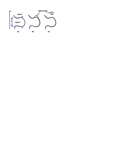
Figure 4: Process of bubble formation from vapour layer in a well-stirred system.

The growth of the vapour layer is limited by its buoyancy; when the layer becomes too thick, vapour driven upwards by the pressure gradient can seepage along the layer quite efficiently and forms bubbles (see Fig. 4). Separating from the layer these bubbles entrain vapour from it and thus effectively reset the layer to the zero-thickness state. In Ref. Pimenova-Goldobin-JETP-2014 this process was considered in detail for the symmetric case and the consideration can be plainly repeated for the non-symmetric case we consider here. With this consideration one can find the characteristic contribution of the Poiseuille’s viscous seepage of vapour along a thin layer into the layer thickness derivative $\dot{L}$:

$$\dot{L}_{p}\approx-\frac{(\rho_{l1}+\rho_{l2})gL^{3}}{96\,\eta_{12}}\left(\frac{\delta{S}}{\delta{V}}\right)\,,$$

where $\eta_{12}$ is the dynamic viscosity of vapour, $g$ is the gravity, $\rho_{j}$ are the densities of liquids.

One can notice, that $\dot{L}_{p}$ strongly depends on the layer thickness, $\dot{L}_{p}\propto L^{3}$, as compared to the growth owned by evaporation, which has a constant rate $\dot{L}$. For this reason, one can neglect the role of the vapour seepage at early stage and consider that the vapour layer breaks away when $\dot{L}_{p}$ becomes equal to the evaporational growth rate. Hence, the vapour layer thickness attained before the breakaway is

$$L_{\ast}\approx\left[\frac{96\,\eta_{12}}{(\rho_{l1}+\rho_{l2})g}\left(\frac{\delta{S}}{\delta{V}}\right)^{-1}\dot{L}\right]^{1/3}\,,$$

which corresponds to the time instant

$$t_{\ast}\approx\frac{L_{\ast}}{\dot{L}}\approx\left[\frac{96\,\eta_{12}}{(\rho_{l1}+\rho_{l2})g}\left(\frac{\delta{S}}{\delta{V}}\right)^{-1}\right]^{1/3}\dot{L}^{-2/3}.$$ (32)

It should be noted that when the vapour layer breaks away, some overheating of liquid, related to the linear in time term in Eqs. (29)–(30), remains in the vicinity of the layer. However, for the symmetric case, the heat of this overheating was revealed to make a negligible contribution into the net heat balance Pimenova-Goldobin-JETP-2014 . For the asymmetric case the orders of magnitude of values are the same and this overheat can be also neglected; suggesting that after breakaway the interface state is reset to the state (29)–(30) with $t=0$ and $L=0$.

With the known reference time instant $t_{\ast}$ of the vapour layer resetting, one can evaluate the characteristic maximal temperature in components attained at the maximal distance from the interface, $z_{j,\mathrm{max}}\sim H_{j}$, at $t=t_{\ast}$. Eq. (29) yields

$$\Theta_{2,\mathrm{max}}= \frac{n_{1\ast}^{(0)}n_{2\ast}^{(0)}\,\dot{L}^{2}}{(\gamma_{1}+\gamma_{2})D_{12}n_{0\ast}}t_{\ast}$$

$${}+\frac{\Lambda_{1}n_{1*}^{(0)}+\Lambda_{2}n_{2*}^{(0)}}{2n_{2*}^{(0)}c_{p,l2}}\left[1-\frac{\dot{q}_{S}}{\dot{Q}_{S}}\right]Z_{2,\mathrm{max}}$$

$${}+\frac{1}{2}\frac{n_{l2}^{2}\,n_{1\ast}^{(0)}}{(\gamma_{1}+\gamma_{2})\,n_{0\ast}\,n_{2\ast}^{(0)}}\frac{\chi_{2}}{D_{12}}Z_{2,\mathrm{max}}^{2}$$ (33)

$$=\Theta_{4/3}Z_{\mathrm{max}}^{4/3}+\left[1-\frac{\dot{q}_{S}}{\dot{Q}_{S}}\right]\Theta_{2,1}Z_{\mathrm{max}}+\Theta_{2,2}Z_{\mathrm{max}}^{2}\,,$$ (34)

where, in accordance to Eqs. (32), (26) and (31),

$$Z_{\mathrm{max}} =Z_{1,\mathrm{max}}+Z_{2,\mathrm{max}}$$

$$=\left(\frac{n_{1*}^{(0)}}{n_{l1}}\frac{\phi_{1}}{\chi_{1}}+\frac{n_{2*}^{(0)}}{n_{l2}}\frac{\phi_{2}}{\chi_{2}}\right)\frac{\dot{L}}{(\delta{S}/\delta{V})}$$ (35)

is introduced so that

$$Z_{j,\mathrm{max}}=\psi_{j}Z_{\mathrm{max}}\,,\qquad\psi_{j}=\frac{\frac{n_{j*}^{(0)}}{n_{lj}}\frac{\phi_{j}}{\chi_{j}}}{\frac{n_{1*}^{(0)}}{n_{l1}}\frac{\phi_{1}}{\chi_{1}}+\frac{n_{2*}^{(0)}}{n_{l2}}\frac{\phi_{2}}{\chi_{2}}}\,,$$

and

$$\Theta_{4/3}=\frac{\displaystyle\frac{n_{1\ast}^{(0)}n_{2\ast}^{(0)}}{(\gamma_{1}+\gamma_{2})D_{12}n_{0\ast}}\left(\frac{96\,\eta_{12}}{(\rho_{1}+\rho_{2})g}\right)^{1/3}\frac{\delta{S}}{\delta{V}}}{\displaystyle\left(\frac{n_{1*}^{(0)}}{n_{l1}}\frac{\phi_{1}}{\chi_{1}}+\frac{n_{2*}^{(0)}}{n_{l2}}\frac{\phi_{2}}{\chi_{2}}\right)^{4/3}}\,,$$ (36)

$$\Theta_{j,1}=\frac{\Lambda_{1}n_{1*}^{(0)}+\Lambda_{2}n_{2*}^{(0)}}{2n_{j*}^{(0)}c_{p,lj}}\,\psi_{j}\,,$$ (37)

$$\Theta_{j,2}=\frac{1}{2}\frac{n_{lj}^{2}\,n_{2-j\,\ast}^{(0)}}{(\gamma_{1}+\gamma_{2})\,n_{0\ast}\,n_{j\ast}^{(0)}}\frac{\chi_{j}}{D_{12}}\,\psi_{j}^{2}\,.$$ (38)

Similarly to Eq. (34), the characteristic maximal temperature of the component 1 can be written down;

$$\Theta_{1,\mathrm{max}}=\Theta_{4/3}Z_{\mathrm{max}}^{4/3}+\left[1+\frac{\dot{q}_{S}}{\dot{Q}_{S}}\right]\Theta_{1,1}Z_{\mathrm{max}}+\Theta_{1,2}Z_{\mathrm{max}}^{2}\,.$$ (39)

As discussed above, after breakaway of the vapour layer, one can approximately assume the interface and its vicinity to be reset to the early stage of the vapour-layer-growth solution, when $L\ll L_{\ast}$. Then the average over time and space values of terms in Eqs. (29)–(30) are determined by the averages $\langle{t}\rangle=t_{\ast}/2$ and $\langle{z^{n}}\rangle=z_{\mathrm{max}}^{n}/(n+1)$;

$$\langle\Theta_{1}\rangle= \frac{\Theta_{4/3}}{2}Z_{\mathrm{max}}^{4/3}+\left[1+\frac{\dot{q}_{S}}{\dot{Q}_{S}}\right]\frac{\Theta_{1,1}}{2}Z_{\mathrm{max}}+\frac{\Theta_{1,2}}{3}Z_{\mathrm{max}}^{2}\,,$$ (40)

$$\langle\Theta_{2}\rangle= \frac{\Theta_{4/3}}{2}Z_{\mathrm{max}}^{4/3}+\left[1-\frac{\dot{q}_{S}}{\dot{Q}_{S}}\right]\frac{\Theta_{2,1}}{2}Z_{\mathrm{max}}+\frac{\Theta_{2,2}}{3}Z_{\mathrm{max}}^{2}\,.$$ (41)

Eqs. (34), (39), (40), and (41) provide relations between the system state variables and the variables $\dot{L}$ (or $Z_{\mathrm{max}}$, see Eq. (35)) and heat inflow asymmetry $(\dot{q}_{S}/\dot{Q}_{S})$. While the latter two are not accessible for direct control, the former can be manipulated directly. Given $\Theta_{j,\mathrm{max}}$ are maintained to be fixed, $(\dot{q}_{S}/\dot{Q}_{S})$ and $Z_{\mathrm{max}}$ can be calculated from Eqs. (34) and (39); the equation

$$\frac{\Theta_{1,\mathrm{max}}}{\Theta_{1,1}}+\frac{\Theta_{2,\mathrm{max}}}{\Theta_{2,1}}=\left(\frac{1}{\Theta_{1,1}}+\frac{1}{\Theta_{2,1}}\right)\Theta_{4/3}Z_{\mathrm{max}}^{4/3}\quad$$

$${}+2Z_{\mathrm{max}}+\left(\frac{\Theta_{1,2}}{\Theta_{1,1}}+\frac{\Theta_{2,2}}{\Theta_{2,1}}\right)Z_{\mathrm{max}}^{2}$$ (42)

governs $Z_{\mathrm{max}}$ and, with calculated $Z_{\mathrm{max}}$, one can straightforwardly find $(\dot{q}_{S}/\dot{Q}_{S})$ from Eq. (34) or (39). Similarly, given $\langle\Theta_{j}\rangle$ are maintained to be fixed,

$$\frac{\langle\Theta_{1}\rangle}{\Theta_{1,1}}+\frac{\langle\Theta_{2}\rangle}{\Theta_{2,1}}=\left(\frac{1}{\Theta_{1,1}}+\frac{1}{\Theta_{2,1}}\right)\frac{\Theta_{4/3}}{2}Z_{\mathrm{max}}^{4/3}\qquad$$

$${}+Z_{\mathrm{max}}+\frac{1}{3}\left(\frac{\Theta_{1,2}}{\Theta_{1,1}}+\frac{\Theta_{2,2}}{\Theta_{2,1}}\right)Z_{\mathrm{max}}^{2}\,.$$ (43)

5.1.2 Case of stratified system

The process of boiling can be not strong enough for the rising vapour bubbles to enforce any significant stirring of the system. For instance, one can observe such a behaviour of the system in Figs. 1(b) and 2(a). In this case system is well stratified; the light liquid rests upon the heavy one with mainly unperturbed interface. The breakaway of the vapour layer in such a system is related to the Rayleigh–Taylor instability Rayleigh-1883 ; Taylor-1950 of the upper vapour–water interface (one can see Fig. 5 in Appendix C), which is gravitationally unstable.

However, our case is significantly different compared to the conventional Rayleigh–Taylor instability; we deal with an extremely thin vapour layer in between of two liquids, without which the system is stably stratified. This specific case of Rayleigh–Taylor instability is actualised by our problem setup and, to the authors’ knowledge, was not addressed in the literature; the consideration of this instability is provided in Appendix C. Without vapour generation, the exponential growth rate of the most dangerous perturbations is accurately given by Eq. (92);

$$\lambda_{1}=\frac{L^{3}}{54\eta_{12}}\frac{\sigma_{1}\sigma_{2}}{\sigma_{1}+\sigma_{2}}\frac{k_{1}^{4}(k_{2}^{2}+k_{1}^{2}/3)}{k_{12}^{2}+k_{1}^{2}/3}\,,$$ (44)

where $\sigma_{j}$ are the surface tension coefficients for vapour–liquid interfaces and $k_{1}$, $k_{2}$, and $k_{12}$ are given by Eqs. (88). To be able to track the physical meaning of terms in the latter equation, we introduce $\tilde{\sigma}=\sigma_{1}\sigma_{2}/(\sigma_{1}+\sigma_{2})$ and $\tilde{\rho}$ in a way that $(\tilde{\rho}{g}/\tilde{\sigma})^{2}=k_{1}^{4}(k_{2}^{2}+k_{1}^{2}/3)/(k_{12}^{2}+k_{1}^{2}/3)$ (compare to Eqs. (88)). Then, Eq. (44) reads

$$\lambda_{1}=\frac{L^{3}(\tilde{\rho}g)^{2}}{54\eta_{12}\tilde{\sigma}}\,.$$

The reference time of hydrodynamic instability development $t_{\ast}\sim 1/\lambda_{1}\propto L^{-3}$. Again, one can notice the instability development to be very slow for small $L$ and extremely fast for large $L$. In the same spirit as for the previous case, we assume the vapour layer to growth with negligible effect of the instability until the instability development time $t_{\ast}$ becomes commensurable to the layer growth time $L/\dot{L}$ and fast layer breakaway happens. Thus,

$$t_{\ast}=\frac{54\eta_{12}\tilde{\sigma}}{(\dot{L}t_{\ast})^{3}(\tilde{\rho}g)^{2}}\,,$$

and one finds

$$t_{\ast}=\frac{(54\eta_{12}\tilde{\sigma})^{1/4}}{(\tilde{\rho}g)^{1/2}}\dot{L}^{-3/4}\,.$$ (45)

Noteworthy, this case is featured by a different power law of dependence $t_{\ast}(\dot{L})$ than in Eq. (32).

With the reference time $t_{\ast}$ of the vapour layer resetting given by Eq. (45), one can evaluate the characteristic maximal temperature in components similarly to the case of a well-stirred system. Eqs. (29) and (30) yield for a stratified system

$$\Theta_{1,\mathrm{max}}= \Theta_{5/4}Z_{\mathrm{max}}^{5/4}+\left[1+\frac{\dot{q}_{S}}{\dot{Q}_{S}}\right]\Theta_{1,1}Z_{\mathrm{max}}+\Theta_{1,2}Z_{\mathrm{max}}^{2}\,,$$ (46)

$$\Theta_{2,\mathrm{max}}= \Theta_{5/4}Z_{\mathrm{max}}^{5/4}+\left[1-\frac{\dot{q}_{S}}{\dot{Q}_{S}}\right]\Theta_{2,1}Z_{\mathrm{max}}+\Theta_{2,2}Z_{\mathrm{max}}^{2}\,,$$ (47)

where

$$\Theta_{5/4}=\frac{\displaystyle\frac{n_{1\ast}^{(0)}n_{2\ast}^{(0)}}{(\gamma_{1}+\gamma_{2})D_{12}n_{0\ast}}\frac{(54\eta_{12}\tilde{\sigma})^{1/4}}{(\tilde{\rho}g)^{1/2}}\left(\frac{\delta{S}}{\delta{V}}\right)^{5/4}}{\displaystyle\left(\frac{n_{1*}^{(0)}}{n_{l1}}\frac{\phi_{1}}{\chi_{1}}+\frac{n_{2*}^{(0)}}{n_{l2}}\frac{\phi_{2}}{\chi_{2}}\right)^{5/4}}\,.$$ (48)

Note, for this case it is more suitable to express volumetric fractions $\phi_{j}$ of components in terms of well determined parameters $H_{j}$, which are the thicknesses of two liquid layers; $\phi_{j}=H_{j}/(H_{1}+H_{2})$.

Mean temperatures are

$$\langle\Theta_{1}\rangle= \frac{\Theta_{5/4}}{2}Z_{\mathrm{max}}^{5/4}+\left[1+\frac{\dot{q}_{S}}{\dot{Q}_{S}}\right]\frac{\Theta_{1,1}}{2}Z_{\mathrm{max}}+\frac{\Theta_{1,2}}{3}Z_{\mathrm{max}}^{2}\,,$$ (49)

$$\langle\Theta_{2}\rangle= \frac{\Theta_{5/4}}{2}Z_{\mathrm{max}}^{5/4}+\left[1-\frac{\dot{q}_{S}}{\dot{Q}_{S}}\right]\frac{\Theta_{2,1}}{2}Z_{\mathrm{max}}+\frac{\Theta_{2,2}}{3}Z_{\mathrm{max}}^{2}\,.$$ (50)

For fixed $\Theta_{j,\mathrm{max}}$ or $\langle\Theta_{j}\rangle$, one finds

$$\frac{\Theta_{1,\mathrm{max}}}{\Theta_{1,1}}+\frac{\Theta_{2,\mathrm{max}}}{\Theta_{2,1}}=\left(\frac{1}{\Theta_{1,1}}+\frac{1}{\Theta_{2,1}}\right)\Theta_{5/4}Z_{\mathrm{max}}^{5/4}\quad$$

$${}+2Z_{\mathrm{max}}+\left(\frac{\Theta_{1,2}}{\Theta_{1,1}}+\frac{\Theta_{2,2}}{\Theta_{2,1}}\right)Z_{\mathrm{max}}^{2}\,,$$ (51)

$$\frac{\langle\Theta_{1}\rangle}{\Theta_{1,1}}+\frac{\langle\Theta_{2}\rangle}{\Theta_{2,1}}=\left(\frac{1}{\Theta_{1,1}}+\frac{1}{\Theta_{2,1}}\right)\frac{\Theta_{5/4}}{2}Z_{\mathrm{max}}^{5/4}\qquad$$

$${}+Z_{\mathrm{max}}+\frac{1}{3}\left(\frac{\Theta_{1,2}}{\Theta_{1,1}}+\frac{\Theta_{2,2}}{\Theta_{2,1}}\right)Z_{\mathrm{max}}^{2}\,.$$ (52)

5.2 Vapour generation at constant heat inflow

Let us establish the relation between the system state parameters and the volumetric heat influx

$$\dot{Q}_{V}=\frac{\delta Q}{\delta V\delta t}\,.$$

Corresponding heat influx per unit area of the interface

$$\dot{Q}_{S}=\left(\frac{\delta{S}}{\delta{V}}\right)^{-1}\dot{Q}_{V}.$$

For a statistically stationary process of boiling, mean temperature does not grow and all the heat influx to the system is spent for vapour generation; therefore, Eq. (24) for the relation between $\dot{Q}_{S}$ and $\dot{L}$ is valid. Hence, Eq. (35) reads

$$Z_{\mathrm{max}} =\left(\frac{n_{1*}^{(0)}}{n_{l1}}\frac{\phi_{1}}{\chi_{1}}+\frac{n_{2*}^{(0)}}{n_{l2}}\frac{\phi_{2}}{\chi_{2}}\right)\frac{\dot{L}}{(\delta{S}/\delta{V})}$$

$$=\frac{\displaystyle\left(\frac{n_{1*}^{(0)}}{n_{l1}}\frac{\phi_{1}}{\chi_{1}}+\frac{n_{2*}^{(0)}}{n_{l2}}\frac{\phi_{2}}{\chi_{2}}\right)\frac{\dot{Q}_{V}}{(\delta{S}/\delta{V})^{2}}}{\Lambda_{1}n_{1\ast}^{(0)}+\Lambda_{2}n_{2\ast}^{(0)}}\,.$$ (53)

With this expression for $Z_{\mathrm{max}}$, one can calculate maximal temperatures in components with Eqs. (39), (33) or (46), (47) and mean temperatures with Eqs. (40), (41) or (49), (50) for the cases of well-stirred and stratified systems.

Assessments: Combustion of n-heptane over water.

For combustion of a light flammable liquid over a heavier liquid one can evaluate the conductive heat influx from the burning surface to the interface; $\dot{Q}_{S}\sim\kappa_{1}(T_{1b}-T_{\ast})/H_{1}$, where $T_{1b}$ is the bulk boiling temperature of the burning liquid (see Sec. 2 for explanations why temperature of the surface of the burning liquid must be nearly $T_{1b}$) and $H_{1}$ is the flammable liquid layer thickness. Here, for an estimate, we neglect the heat conduction loss from liquids to the environment. Eq. (24) yields

$$\dot{L} =\frac{\kappa_{1}}{\Lambda_{1}n_{1\ast}^{(0)}+\Lambda_{2}n_{2\ast}^{(0)}}\frac{T_{1b}-T_{\ast}}{H_{1}}$$

$$=\frac{c_{p,l1}n_{l1}\chi_{1}}{\Lambda_{1}n_{1\ast}^{(0)}+\Lambda_{2}n_{2\ast}^{(0)}}\frac{T_{1b}-T_{\ast}}{H_{1}}\approx\frac{1.47\cdot 10^{-6}\mathrm{m^{2}/s}}{H_{1}}\,,$$

where parameter values for n-heptane–water are taken from Tab. 1. With Eq. (45), one can calculate $t_{\ast}\approx 5.53\cdot 10^{-4}\mathrm{m^{3/4}s^{1/4}}\times\dot{L}^{-3/4}$ and find the reference layer thickness $L_{\ast}=\dot{L}t_{\ast}\approx 5.53\cdot 10^{-4}\mathrm{m^{3/4}s^{1/4}}\times\dot{L}^{1/4}\approx 1.93\cdot 10^{-5}\mathrm{m^{5/4}}\times H_{1}^{-1/4}$ at the instant of breakaway. The wavelength of the most dangerous instability mode of a thin vapour layer between the n-heptane and water layers $l_{vl}=2\pi/k_{\mathrm{max}}^{n\mathrm{C_{7}H_{16}-H_{2}O}}\approx 1.46\,\mathrm{cm}$ (see Appendix C). Hence, a vapour bubble separating from the interface is formed from the vapour layer patch of area $S_{vl}\approx l_{vl}^{2}$ and possesses volume $V_{b}\approx S_{vl}L_{\ast}$ or $(\pi/6)d_{b}^{3}$, where $d_{b}$ is the bubble diameter. Finally, the bubble diameter

$$d_{b}\approx[(6/\pi)l_{vl}^{2}L_{\ast}]^{1/3}\approx 2.0\cdot 10^{-3}\mathrm{m^{13/12}}\times H_{1}^{-1/12}\,.$$

One can notice the dependence of $d_{b}$ on $H_{1}$ to be extremely “slow”, power $(-1/12)$; for the layer thickness of order of magnitude of $1\,\mathrm{cm}$ the bubble diameter $d_{b}\approx 2.9\,\mathrm{mm}$, which slightly overestimates the characteristic size observed in Fig. 2(b). This overestimation is expected because we neglected the heat loss to the environment and thus overestimated the heat influx spent for the generation of vapour. Thus our theoretical description of the process yields results which match experimental observations well.

6 Discussion of simplification assumptions

Let us summarise the simplification assumptions made in the course of developing the theory and discuss possible inaccuracies brought in with these assumptions.

$\bullet$ The solution for the transversal structure of the growing vapour layer and its vicinity is derived neglecting the layer curvature and sideway motion of vapour and liquid. The inaccuracy brought in with these neglections is expected to be small by virtue of the smallness of the maximal vapour layer thickness attained before the layer breaks away, which is $L_{\mathrm{max}}\sim 10^{-5}-10^{-4}\,\mathrm{m}$, compared to the shortest scale along the layer, which is $\sim 10^{-3}-10^{-2}\,\mathrm{m}$.

$\bullet$ For the evaporation process we neglect finiteness of the rate of molecule escape from liquid into vapour, assuming the vapour number density immediately above the liquid surface to be equal the saturation vapour one. We provide arguments for this assumption. In the light of final results this assumption can be treated to work well enough as the predicted features of the bubble formation process agree with experimental observations, while for evaporation from open liquid surfaces the finiteness of the escape rate leads to the decrease of the evaporation rate by factor of $10$ (e.g., see Anisimov-Rakhmatulina-1973 ).

$\bullet$ Considering the hydrodynamic instability of the stratified three-layer system, we assume the liquid flow rates to be small compared to the rates of the vapour flow along the vapour layer (see Appendix C). The accuracy of this approximation can be quantified by the ratio of dynamic viscosities of vapour and liquid, $\eta_{12}/\eta_{\mathrm{liq}}\approx 10^{-2}$. The liquid flow is also considered to be inviscid. Indeed, for the instability flow in liquid the characteristic rate $v\sim L_{\mathrm{max}}\lambda_{1,\mathrm{max}}\sim 10^{-3}\,\mathrm{m/s}$ and the corresponding thickness of the viscous boundary layer $h_{\mathrm{v.b.l.}}\sim\nu_{\mathrm{liq}}/v\sim 1\,\mathrm{mm}$ is small compared to the characteristic spatial scale of the instability, which is $1.0-1.5\,\mathrm{cm}$.

$\bullet$ The reference time of the layer breakaway is calculated for two limit cases: a well-stirred system and a well-stratified one. With estimations of Appendix B, one can see that the boiling regime is controlled by the heat inflow rate into the system, material parameters and the system volume. For the conditions of the demonstration experiment with n-heptane–water system (Fig. 2), the system was observed to be rather close to a well-stratified state. For the burning “white spirit”–water system (Fig. 1), we observed all the range of boiling regimes from the one with prominent stratification to a strong stirring.

7 Conclusion

We have theoretically explored the process of boiling at the interface between two immiscible liquids below the bulk boiling temperatures of both components. A comprehensive theoretical description of this process is constructed. The equations of evolution of the vapour layer and temperature fields in liquids within the vicinity of the layer are obtained. The growing-vapour-layer solution to these equations is derived. The vapour layer breakaway due to its buoyancy and consequent vapour bubble formation are described, and the relationships between macroscopic parameters of the boiling system state and the derived solution are established for the cases of a well-stirred system and a stratified system.

The process parameters are evaluated for realistic systems, such as the n-heptane–water one. The relevance of the case we considered is revealed for combustion of a light inflammable liquid over a heavy nonflammable one and demonstrated experimentally for n-heptane–water and “white spirit”–water systems. The theory based results are found to match well the experimental observations for the n-heptane–water system.

The auxiliary problem of the instability of a thin horizontal vapour layer between two liquids to bubble formation has been solved (Appendix C). This solution provides information required for calculation of the characteristic size of bubbles, spatial density of bubble formation centers on the interface, and limitation on the vapour layer thickness which can be attained before the breakaway of vapour layer.

Remarkably, for the problem of the bulk boiling the key question is the rate of nucleation. The answering to this question on the basis of the theoretical consideration without employment of semi-empiric information is a challenging task heavily requiring approaches from the statistical physics theory of nonequilibrium systems Pitaevskii-Lifshitz-v10 and, in particular, the theory of hydrodynamic fluctuations Pitaevskii-Lifshitz-v9 . On the contrast, the theory of boiling of system of immiscible liquids below their bulk boiling points can be constructed from scratch on the mere basis of the macroscopic fluid dynamics.

Appendix A Distribution of species in the vapour layer

In this appendix section we derive the particle number density distribution within a vapour layer linearly growing with time, and demonstrate it to be of nearly linear profile, see Eqs. (19)–(20).

For the idealised symmetric case the problem was found to have an exact solution of the form $L\propto t$, $\Theta\propto t$ with linear profile of the distribution of the particle number densities Pimenova-Goldobin-JETP-2014 . We expect a “successor” of this solution to exist for an asymmetric case. Accordingly, let us seek the solutions to Eqs. (4) with boundary conditions (5)–(8) in the form of a series in polynomials of $z$;

$$n_{1}(z,t)=n_{1\ast}^{(0)}-\gamma_{2}\Theta(t)+\alpha\big{(}z+L_{2}(t)\big{)}\qquad$$

$${}+\beta\big{(}z-L_{1}(t)\big{)}\big{(}z+L_{2}(t)\big{)}+\dots\,,$$ (54)

$$n_{2}(z,t)=n_{2\ast}^{(0)}-\gamma_{1}\Theta(t)-\alpha\big{(}z-L_{1}(t)\big{)}\qquad$$

$${}-\beta\big{(}z-L_{1}(t)\big{)}\big{(}z+L_{2}(t)\big{)}+\dots\,,$$ (55)

and see whether the terms in these series are proportional to powers of a small parameter, allowing one to neglect all terms but the leading ones which are linear functions of $z$. The quadratic in $z$ terms, with coefficient $\beta$, are intentionally constructed so that they vanish at the layer boundaries. Here the boundary conditions (5)–(6) require

$$\alpha=(\gamma_{1}+\gamma_{2})\frac{\Theta}{L}\,,$$ (56)

and, for $\alpha$ constant in time with linearly growing $\Theta$ and $L$, Eqs. (4) yield

$$-\gamma_{2}\dot{\Theta}+\alpha\dot{L}_{2} =2D_{12}\beta\,,$$ (57)

$$-\gamma_{1}\dot{\Theta}+\alpha\dot{L}_{1} =-2D_{12}\beta\,.$$ (58)

On the other hand, Eqs. (9) and (10) yield

$$\dot{L}_{1} =\frac{D_{12}}{n_{2\ast}^{(0)}}(\alpha+\beta L)\,,$$ (59)

$$\dot{L}_{2} =\frac{D_{12}}{n_{1\ast}^{(0)}}(\alpha-\beta L)\,.$$ (60)

Substituting $\Theta=(\gamma_{1}+\gamma_{2})^{-1}\alpha L$ from Eq. (56) and $\dot{L}_{i}$ from (59) and (60) into equation system (57)–(58), one can obtain

$$\beta=\frac{\alpha^{2}}{4}\frac{n_{0\ast}}{n_{1\ast}^{(0)}n_{2\ast}^{(0)}}\left(\frac{n_{2\ast}^{(0)}-n_{1\ast}^{(0)}}{n_{2\ast}^{(0)}+n_{1\ast}^{(0)}}-\frac{\gamma_{2}-\gamma_{1}}{\gamma_{2}+\gamma_{1}}\right)\quad$$

$$\times\left[1+\mathcal{O}\left(\frac{\beta L}{\alpha}\right)\right].$$ (61)

With Eq. (61), one can see

$$\frac{\beta L}{\alpha}\sim\frac{\alpha L}{4n_{0\ast}}=\frac{(\gamma_{1}+\gamma_{2})\Theta}{4n_{0\ast}}$$

which is small as required for the series (54) and (55) to be series in a small parameter $(\gamma_{1}+\gamma_{2})\Theta/n_{0\ast}$. The cubic in $z$ term in series (54) and (55) can be further demonstrated to be small compared to the quadratic term. Thus, for the leading order of accuracy, it is enough to keep the linear in $z$ terms in Eqs. (54) and (55) and neglect the quadratic and higher ones.

Notice, according to Eq. (61), $\beta$ exactly vanishes for $n_{2\ast}^{(0)}/n_{1\ast}^{(0)}=\gamma_{2}/\gamma_{1}$ and the linear profile solution becomes an exact one. More generally, for the special case of $n_{2}^{(0)}(T)/n_{1}^{(0)}(T)=const$, the linear-profile solution is exact for arbitrary overheating.

Appendix B Assessment of the dependence of $(\delta{S}/\delta{V})$ on the heat influx for a well-stirred system

In this appendix section we attempt to derive the rough relationships between the macroscopic parameter $(\delta{S}/\delta{V})$ of the system state and the heat influx rate per unit volume $\dot{Q}_{V}=\delta{Q}/(\delta{V}\delta{t})$ for a statistically stationary process of interfacial boiling.

The flow and consequent stirring in the system are enforced by the buoyancy of the vapour bubbles, while other mechanisms counteract the stirring of the system. These other mechanisms are gravitational stratification of two liquids, surface tension tending to minimise the interface area and viscous dissipation of the flow energy. Since the latent heat of phase transitions and heat of temperature inhomogeneities are enormously large compared to the realistic values of the kinetic energy of microscopic motion and gravitational potential energy[], the latter can be neglected in consideration of the heat balance. Hence, all the heat inflow into the system can be considered to be spent for the vapour generation; $\dot{Q}_{V}V\longrightarrow(\Lambda_{1}n_{1\ast}^{(0)}+\Lambda_{2}n_{2\ast}^{(0)})\dot{V}_{v}$, where $V$ is the system volume, and $\dot{V}_{v}$ is the volume of the vapour produced in the system per unit time. Thus,

$$\dot{V}_{v}=\frac{\dot{Q}_{V}\,V}{\Lambda_{1}n_{1\ast}^{(0)}+\Lambda_{2}n_{2\ast}^{(0)}}\,.$$ (62)

The potential energy of buoyancy of rising vapour bubbles $\rho_{l}V_{v}gh/2$ (where $h$ is the linear size of the system, $h\sim V^{1/3}$, $\rho_{l}$ is the average density of liquids, the vapour density is zero compared to the liquid density) is converted into the kinetic energy of liquid flow, the potential energy of a stirred state of the two-liquid system, the surface tension energy and dissipated by viscosity forces. In a statistically stationary state, the mechanical kinetic and potential energies do not change averagely over time and all the energy influx is to be dissipated by viscosity;

$$\rho_{l}V_{v}gh/2\longrightarrow\dot{W}_{l,k}\tau\,,$$

where $\dot{W}_{l,k}$ is the rate of viscous dissipation of energy, $\tau$ is the time of generation of the vapour volume $V_{v}$, $V_{v}=\dot{V}_{v}\tau$. Hence,

$$\rho_{l}\dot{V}_{v}g\frac{h}{2}\sim\dot{W}_{l,k}\,.$$ (63)

Let us estimate the viscous dissipation of the kinetic energy of flow $W_{l,k}$;

$$\dot{W}_{l,k} =\int\limits_{V}\vec{v}\cdot\vec{f}_{\mathrm{vis}}\mathrm{d}V\sim\int\limits_{V}\vec{v}\cdot\left(-\eta_{l}\frac{\vec{v}}{H^{2}}\right)\mathrm{d}V$$

$$\sim -\frac{\eta_{l}}{\rho_{l}}\frac{2}{\left(\frac{H_{1}+H_{2}}{2}\right)^{2}}\int\limits_{V}\frac{\rho_{l}v^{2}}{2}\mathrm{d}V\sim-8\nu_{l}\left(\frac{\delta{S}}{\delta{V}}\right)^{2}W_{l,k}\,.$$ (64)

Here $\vec{v}$ is the liquid velocity, $\vec{f}_{\mathrm{vis}}$ is the viscous force per unit volume, $H$ is the spatial scale of flow inhomogeneity, which is the half-distance between the sheets of the folded interface between liquid components, $\eta_{l}$ and $\nu_{l}$ are the characteristic dynamic and kinematic viscosities of liquids, respectively.

Further, we have to establish the relationship between the flow kinetic energy and the mechanical potential energy in the system. Rising vapour bubbles pump the mechanical energy into the system, while its stochastic dynamics is governed by interplay of its flow momentum and the forces of the gravity and the surface tension on the interface. In thermodynamic equilibrium, the total energy is strictly equally distributed between potential and kinetic energies related to quadratic terms in Hamiltonian (this statement is frequently simplified to a less accurate statement, that energy is equally distributed between kinetic and potential energies associated with each degree of freedom). Being not exactly in the case where one can rigorously speak of thermalization of the stochastic Hamiltonian system dynamics, we still may assess the kinetic energy of flow to be of the same order of magnitude as the mechanical potential energy of the system. Thus,

$$W_{l,k}\sim W_{l,pg}+W_{l,p\sigma}\,,$$ (65)

where $W_{l,pg}$ and $W_{l,p\sigma}$ are the gravitational potential energy and the surface tension energy, respectively. We set the zero levels of these potential energies at the stratified state of the system with a flat horizontal interface.

The gravitational potential energy of the well-stirred state with uniform distribution of two phases over hight is

$$W_{l,pg}\sim\Delta\rho_{l}Vg\frac{h}{2}\,,$$

where $\Delta\rho_{l}$ is the component density difference. The surface tension energy is

$$W_{l,p\sigma}\sim(\sigma_{1}+\sigma_{2})V\left(\frac{\delta{S}}{\delta{V}}\right)\,,$$

where we neglected the interface area of the stratified state compared to the area $V(\delta{S}/\delta{V})$ in the well-stirred state. Due to the presence of the vapour layer between liquids the effective surface tension coefficient of the interface is $(\sigma_{1}+\sigma_{2})$ but not $\sigma_{12}$ as it would be in the absence of the vapour layer.

Collecting Eqs. (62)–(65), one finds

$$\rho_{l}\frac{\dot{Q}_{V}\,V}{\Lambda_{1}n_{1\ast}^{(0)}+\Lambda_{2}n_{2\ast}^{(0)}}g\frac{h}{2}$$

$$\quad\approx 8\nu_{l}\left(\frac{\delta{S}}{\delta{V}}\right)^{2}\left[\Delta\rho_{l}Vg\frac{h}{2}+(\sigma_{1}+\sigma_{2})V\left(\frac{\delta{S}}{\delta{V}}\right)\right]\,.$$

This equation can be simplified to

$$\dot{Q}_{V}\approx B\left(\frac{\delta{S}}{\delta{V}}\right)^{2}\left[1+\frac{2}{k_{12}^{2}h}\left(\frac{\delta{S}}{\delta{V}}\right)\right]\,,$$ (66)

where $B=8\nu_{l}(\Lambda_{1}n_{1\ast}^{(0)}+\Lambda_{2}n_{2\ast}^{(0)})\Delta\rho_{l}/\rho_{l}$ and $k_{12}$ is given by Eq. (88). Noteworthy, the relative importance of the first and second terms in the brackets in Eq. (66) depends on the system size $h$.

For the n-heptane–water system, $B\approx 1.5\,\mathrm{J/(m\cdot s)}$ and $l_{k_{12}}\equiv 1/k_{12}\approx 0.5\,\mathrm{cm}$. For a well-stirred system the distance between sheets of the folded interface $(\delta{S}/\delta{V})^{-1}\ll h$. The average compound of these two values can be either small or large compared to $l_{k_{12}}$;
(1) $h\cdot(\delta{S}/\delta{V})^{-1}\ll l_{k_{12}}^{2}$ corresponds to the case of the surface tension dominated system,
(2) $h\cdot(\delta{S}/\delta{V})^{-1}\gg l_{k_{12}}^{2}$ corresponds to the case of a gravity-driven system.

Cubic equation (66) possesses only one positive solution which is real-valued for any value of $\dot{Q}_{V}/B$;

$$\left(\frac{\delta{S}}{\delta{V}}\right)=\left(\frac{\delta{S}}{\delta{V}}\right)_{g}\cdot G\left(\frac{\big{(}\dot{Q}_{V}/B\big{)}^{1/2}}{k_{12}^{2}V^{1/3}}\right),$$ (67)

where $(\delta{S}/\delta{V})_{g}=(\dot{Q}_{V}/B)^{1/2}$ is the value of parameter $(\delta{S}/\delta{V})$ for a gravity-driven system and function $G(s)=(6s)^{-1}(R+R^{-1}-1)$, $R=(\sqrt{27}s+\sqrt{27s^{2}-1})^{2/3}$; $G(0)=1$ and $G(s\gg 1)=(2s)^{-1/3}$.

Expression (67) allows estimating the value of parameter $(\delta{S}/\delta{V})$ as a function of heat influx $\dot{Q}_{V}$ to the system.

Appendix C Gravitational instability of the vapour layer in stratified system

In this appendix section we discuss the scenario of vapour layer breakaway for the case of the stratified system as in demonstration experiment in Fig. 2. In this case the breakaway of the vapour layer is related to a kind of Rayleigh–Taylor instability Rayleigh-1883 ; Taylor-1950 of the upper liquid–vapour interface, where a heavy liquid lies above a nearly weightless fluid. However, our case is untypical, as we are interested specifically in the case of a gas layer between two liquids, and, which is more peculiar, this layer is extremely thin for the situations of our interest (in the next paragraph we will estimate the characteristic thickness of the vapour layer). Practically, this problem would even not arise without the process of vapour layer formation on the two-liquid contact interface, as there seems to be no other robust mechanism of appearance and persistent maintenance of such a thin layer. To the authors’ knowledge, this problem is not addressed in the literature.

In order to estimate the reference thickness of the layer, one can look at Fig. 2. In Fig. 2(b), the typical diameter of vapour bubbles detaching the interface is $d_{b}\sim 1\,\mathrm{mm}$ and the bubble lanes stand at characteristic distance of $1\,\mathrm{cm}$ from each other, i.e., each bubble is formed by the vapour layer patch breaking-away from the interface area $S_{vl}\sim 1\,\mathrm{cm}^{2}$. The bubble volume $V_{b}=(\pi/6)d_{b}^{3}$ is equal to the layer patch volume $h_{vl}S_{vl}$; therefore, the characteristic thickness of the vapour layer $h_{vl}=V_{b}/S_{vl}\sim 10^{-5}\mathrm{m}$.

All the consideration in this section in focused on the specific fluid dynamical problem and only the final results are employed in the main paper. Thus, for the convenience reason, in this section we will use notations independent of the notations in the main paper.

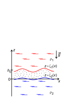
Figure 5: System of two liquids with densities $\rho_{1}$ and $\rho_{2}>\rho_{1}$ separated by a thin layer of viscous gas.

We consider the gravity-capillary waves and the system instability to their growth. For the linear stability analysis it is enough to consider plane-wave perturbations, i.e., the problem can be investigated in the $(x,z)$-geometry, where $z$ is the vertical coordinate and $x$ is the coordinate along the wave vector (see Fig. 5). We consider thicknesses of liquid layers to be large compared to the interface inflection wavelength, in which case one can assume the unperturbed liquids to occupy half-spaces $z>h_{0}$ and $z<0$. The densities of the upper light liquid and the lower heavy liquid are $\rho_{1}$ and $\rho_{2}>\rho_{1}$, respectively, and the vapour is nearly weightless. The positions of the vapour-liquid interfaces are $z=\zeta_{1}(x,t)$ and $z=\zeta_{2}(x,t)$ (Fig. 5); for the unperturbed state $\zeta_{1}=h_{0}$ and $\zeta_{2}=0$, where $h_{0}$ is the unperturbed vapour layer thickness.

The classical marginal Rayleigh–Taylor instability (with no vapour layer) is monotonous and, therefore, the instability threshold is unaffected by viscosity. The problem can be considered for inviscid liquids. The density of the vapour between liquids is nearly zero compared to the liquid densities and its flow should be inertialess. On the other hand, the difference $\dot{\zeta}_{1}-\dot{\zeta}_{2}=\dot{h}$ forces vapour redistribution and can create a strong flow in a narrow gap, which, in the absence of inertia, is restrained only by viscosity. Hence, the viscosity has to be accounted for the vapour layer. Characteristic hydrostatic and hydrodynamic pressure gradients in the system are small compared to atmospheric pressure and one can treat the vapour to be incompressible. Summarizing, we deal with a system where the liquid flow can be assumed inviscid while the vapour flow is incompressible and dominantly viscous, its velocity is much larger than that of liquids.

Let us consider flow in the vapour layer. The layer thickness $h=\zeta_{1}-\zeta_{2}$ is small compared to the characteristic horizontal scale of the wave pattern and hence the flow is nearly parallel to the layer middle surface and pressure is nearly constant across the layer, $p_{g}(x,z)=p_{g}(x)$. Additionally, since the vapour flow is much faster that the liquid flows, one can adopt zero-velocity boundary conditions for the vapour. Thus, one can find the vapour viscous flow to be a Poiseuille flow along a thin gap between two planes:

$$v(x,z)=v_{m}(x)\left(1-\frac{4(z-\zeta_{m})^{2}}{h^{2}}\right)\,,$$ (68)

where $v$ is the vapour velocity tangential to the layer middle surface, $\zeta_{m}=(\zeta_{1}+\zeta_{2})/2$ is the $z$-coordinate of the layer middle surface, $v_{m}$ is the vapour velocity at $\zeta_{m}$. The Navier-Stokes equation for vanishing fluid density provides relation between the flow and the pressure gradient;

$$\frac{\partial}{\partial x}p_{g}(x,t)=\eta\frac{\partial^{2}v}{\partial z^{2}}=-\frac{8\eta}{h^{2}}v_{m}(x,t)\,,$$ (69)

where $p_{g}$ is pressure within the layer, $\eta$ is the dynamic viscosity. The layer thickness change $\dot{h}$ is owned by the fluid flux through the layer cross-section $Q=\int_{\zeta_{1}}^{\zeta_{2}}v\,\mathrm{d}z=(2/3)v_{m}h$; $\dot{h}=-(\partial/\partial x)Q$. Using the relation between $v_{m}$ and pressure gradient (69), one can write

$$\dot{h}=\frac{\partial}{\partial x}\left(\frac{h^{3}}{12\eta}\frac{\partial p_{g}}{\partial x}\right).$$

Since we are to consider infinitesimal perturbations of the state with flat interfaces, we need only contributions which are linear in small parameters $(p_{g}-p_{g0})$ and $(h-h_{0})$;

$$\dot{h}=\frac{h_{0}^{3}}{12\eta}\frac{\partial^{2}p_{g}}{\partial x^{2}}.$$ (70)

Let us now consider the mechanics of liquid phases. Considering inviscid flow, one can describe the current velocity with the stream scalar potential $\Phi_{j}$; the $j$-th liquid velocity $\vec{v}_{j}=\nabla\Phi_{j}$. The incompressibility condition

$$\nabla\cdot\vec{v}_{j}=0$$

requires $\Phi_{j}$ to be harmonic functions;

$$\mathrm{\Delta}\Phi_{j}(x,z,t)=0\,.$$ (71)

The Euler equation in terms of potential takes the form

$$\rho_{j}\nabla\left(\dot{\Phi}_{j}+\frac{1}{2}(\nabla\Phi_{j})^{2}\right)=-\nabla(p_{j}+\rho_{j}gz)\,,$$

where $p_{j}$ is the pressure field in the $j$-th liquid, $g$ is the gravity. Thus, one can evaluate the pressure field for a given flow;

$$p_{j}=p_{j,0}-\rho_{j}\dot{\Phi}_{j}-\rho_{j}gz\,,$$ (72)

where the quadratic term is neglected because we consider an infinitesimal perturbation flow.

The condition of stress balance at the liquid surfaces relates the pressure jump across the surface with the capillary pressure;

$$(p_{1}-p_{g})|_{z=\zeta_{1}} =\sigma_{1}\frac{\partial^{2}\zeta_{1}}{\partial x^{2}}\,,$$ (73)

$$(p_{2}-p_{g})|_{z=\zeta_{2}} =-\sigma_{2}\frac{\partial^{2}\zeta_{2}}{\partial x^{2}}\,,$$ (74)

where $\sigma_{j}$ is the surface tension of the $j$-th liquid.

Since we treat the stability of the flat-interface state and consider small perturbations, it is convenient to formulate equations in domains $z<0$ and $z>h_{0}$ rather than in domains $z<\zeta_{2}$ and $z>\zeta_{1}$. Consequently, the boundary conditions should be moved to $z=0$ and $z=h_{0}$ from $z=\zeta_{2}$ and $z=\zeta_{1}$, respectively. To do so for boundary conditions (73)–(74), one has to employ Eq. (72). Up to the linear in perturbation terms, boundary conditions (73)–(74) can be recast into the following form:

$$-\rho_{1}\dot{\Phi}_{1}|_{z=h_{0}}-p_{g}-\rho_{1}g(\zeta_{1}-h_{0})=\sigma_{1}\frac{\partial^{2}\zeta_{1}}{\partial x^{2}}\,,$$ (75)

$$-\rho_{2}\dot{\Phi}_{2}|_{z=0}-p_{g}-\rho_{2}g\zeta_{2}=-\sigma_{2}\frac{\partial^{2}\zeta_{2}}{\partial x^{2}}\,.$$ (76)

The kinematic boundary conditions remain to be accounted for. The liquid flow shifts the liquid–vapour interface; $\dot{\zeta}_{j}$ is determined by the $z$-component of $j$-th liquid velocity on the liquid surface, in terms of potential,

$$\dot{\zeta_{1}} =\left.\frac{\partial\Phi_{1}}{\partial z}\right|_{z=h_{0}},$$ (77)

$$\dot{\zeta_{2}} =\left.\frac{\partial\Phi_{2}}{\partial z}\right|_{z=0}.$$ (78)

Substituting the thickness variation $\dot{h}=\dot{\zeta_{1}}-\dot{\zeta_{2}}$ in Eq. (70), one finds

$$\dot{\zeta_{1}}-\dot{\zeta_{2}}=\frac{h_{0}^{3}}{12\eta}\frac{\partial^{2}p_{g}}{\partial x^{2}}.$$ (79)

Eqs. (71), (75)–(79) form a complete system of differential equations for fields $\Phi_{j}(x,z,t)$, $\zeta_{j}(x,t)$ and $p_{g}(x,t)$. As the equations for perturbations are homogeneous in the $x$-direction and in time, the solution can be sought in a normal form $\propto e^{\lambda t+ikx}$. For $\Phi_{j}\propto e^{ikx}$, Eq. (71) yields $\Phi_{1}\propto e^{-kz+ikx}$ and $\Phi_{2}\propto e^{kz+ikx}$. Hence, Eqs. (77) and (78) yield $\Phi_{1}|_{z=h_{0}}=-k^{-1}\dot{\zeta}_{1}$ and $\Phi_{2}|_{z=0}=k^{-1}\dot{\zeta}_{2}$, respectively. With substitution of $\Phi_{j}$ and normal perturbation

$$\{\zeta_{1},\zeta_{2}-h_{0},p_{g}\}=\{\xi_{1},\xi_{2},P\}\,e^{\lambda t+ikx},$$

Eqs. (75), (76) and (79) can be cast into the following equation system for amplitudes $\xi_{1}$, $\xi_{2}$, $P$:

$$\left(\rho_{1}\frac{\lambda^{2}}{k}-\rho_{1}g+\sigma_{1}k^{2}\right)\xi_{1}-P =0\,,$$ (80)

$$\left(-\rho_{2}\frac{\lambda^{2}}{k}-\rho_{2}g-\sigma_{2}k^{2}\right)\xi_{2}-P =0\,,$$ (81)

$$\lambda\xi_{1}-\lambda\xi_{2}+\frac{h_{0}^{3}}{12\eta}k^{2}P =0\,.$$ (82)

The corresponding characteristic equation for the exponential growth rate $\lambda$ reads

$$\lambda\left(\lambda^{2}+\frac{\rho_{2}-\rho_{1}}{\rho_{2}+\rho_{1}}gk+\frac{\sigma_{1}+\sigma_{2}}{\rho_{2}+\rho_{1}}k^{3}\right)$$

$$\quad{}+Ak\left(\lambda^{2}-gk+\frac{\sigma_{1}}{\rho_{1}}k^{3}\right)\left(\lambda^{2}+gk+\frac{\sigma_{2}}{\rho_{2}}k^{3}\right)=0\,,$$ (83)

where

$$A=\frac{h_{0}^{3}}{12\eta}\frac{\rho_{1}\rho_{2}}{\rho_{1}+\rho_{2}}$$

is the parameter characterising the thickness of the vapour layer.

Result validation: Limiting cases.

One can consider two limiting cases for the system: thin layer ($h_{0}\to 0$) and thick layer ($h_{0}\to\infty$). In the first case the second term in Eq. (83) can be neglected, and the equation yields

$$\lambda =0\,,$$ (84)

$$\lambda^{2} =-\frac{\rho_{2}-\rho_{1}}{\rho_{2}+\rho_{1}}gk-\frac{\sigma_{1}+\sigma_{2}}{\rho_{2}+\rho_{1}}k^{3}\,.$$ (85)

Eq. (85) is exactly the result for gravity-capillary waves for two-liquid system without vapour layer (however, with surface tension $\sigma=\sigma_{1}+\sigma_{2}$) well known in the literature (e.g., Sharp-1984 ). Since the right part of this equation is strictly nonpositive, all exponential growth rates $\lambda$ are imaginary, there is no instability. Eq. (84) represents the fact that for vanishing $h_{0}$ the inhomogeneities of pressure in the vapour layer dissolves infinitely slowly (cf. Eq. (70)) due to diminished viscous flow along vanishingly narrow gap. These pressure $p_{g}$ perturbations form a neutral mode with $\lambda\to 0$ for $h_{0}\to 0$.

In the opposite limiting case, when thickness $h_{0}$ and parameter $A$ are large enough, the first term in Eq. (83) can be neglected and the characteristic equation can be factorised yielding two independent pairs of solutions:

$$\lambda_{1,2}^{2} =kg-\frac{\sigma_{1}}{\rho_{1}}k^{3}\,,$$ (86)

$$\lambda_{3,4}^{2} =-kg-\frac{\sigma_{2}}{\rho_{2}}k^{3}\,.$$ (87)

These solutions correspond to the case of conventional gravity-capillary waves on the liquid–gas interface (cf. Eq. (85)) for the unstable state of the liquid layer over gas, Eq. (86), and for the stable state of gas over liquid, Eq. (87). In this case, vapour layer is thick enough to make the liquid surfaces insensitive to motion of each other. Eq. (87) has only imaginary solutions, as it should be, while Eq. (86) has a pair of real roots for $k<k_{1}$, where $k_{1}=\sqrt{\rho_{1}g/\sigma_{1}}$. Perturbations with positive $\lambda$ grow exponentially, meaning the system is unstable.

It is convenient to introduce reference values of the wavenumber:

$$k_{1}=\sqrt{\frac{\rho_{1}g}{\sigma_{1}}}\,,\quad k_{2}=\sqrt{\frac{\rho_{2}g}{\sigma_{2}}}\,,\quad k_{12}=\sqrt{\frac{(\rho_{2}-\rho_{1})g}{\sigma_{1}+\sigma_{2}}}\,.$$ (88)

The case of small non-zero $h_{0}$.

Solution $\lambda=0$ for $h_{0}=0$ given by Eq. (84) requires an additional subtle treatment as it can be made non-zero and change its sign with arbitrary small corrections. Thus, the case of small but non-zero $h_{0}$ may be not represented by solution (84) for $h_{0}=0$ well.

Let us first calculate the reference values for $\lambda$, $A$, and $k$: $\lambda_{\ast}$, $A_{\ast}$, and $k_{\ast}$. One can notice, that after substitution of $\lambda=0$, Eq. (83) can be satisfied with $k=k_{1}$ regardless of the value of $A$, and this is the only non-zero value of $k$ which satisfies the equation for $\lambda=0$. Thus $\lambda(k)$ crosses the zero point only at $k=k_{1}$. Hence, it is natural to chose

$$k_{\ast}=k_{1}\,.$$

Further, for $k=k_{\ast}$ the reference value of the terms near $\lambda^{2}$ in brackets of Eq. (83) is $gk_{\ast}$, suggesting

$$\lambda_{\ast}=\sqrt{gk_{1}}\,.$$

The first and second terms in Eq. (83) for $k=k_{\ast}$ and $\lambda=\lambda_{\ast}$ are commensurable when $A$ equals the reference value

$$A_{\ast}=\frac{1}{k_{\ast}\lambda_{\ast}}=g^{-1/2}k_{1}^{-3/2}=\left(\frac{\sigma_{1}}{\rho_{1}}\right)^{3/4}g^{-5/4}\,.$$

The corresponding reference value of $h_{0}$ is

$$h_{0\ast}=\left(\frac{12\eta}{g^{5/4}}\frac{\rho_{1}+\rho_{2}}{\rho_{1}\rho_{2}}\right)^{1/3}\left(\frac{\sigma_{1}}{\rho_{1}}\right)^{1/4}.$$ (89)

For the n-heptane–water system as an example, with data from Tab. 1, one finds $k_{1}=659\,\mathrm{m^{-1}}$, i.e., the reference instability wavelength $2\pi/k_{1}=1.0\,\mathrm{cm}$, $A_{\ast}=1.9\cdot 10^{-5}$, $h_{0\ast}=0.15\,\mathrm{mm}$; $k_{2}=389\,\mathrm{m^{-1}}$ and $k_{12}=206\,\mathrm{m^{-1}}$. The previously estimated thickness $h_{vl}\sim 0.01\,\mathrm{mm}$ of the layer suffering bubble breakaway we observed in the experimental demonstration (Fig. 2) is by factor $15$ smaller than $h_{0\ast}$, meaning we can reliably restrict our consideration to the case $h_{0}\ll h_{0\ast}$.

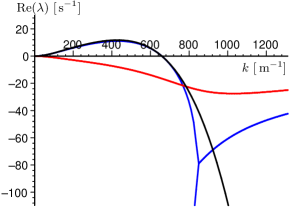
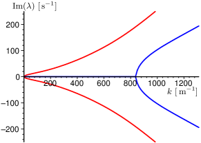
Figure 6: Spectrum of the exponential growth rates $\lambda(k)$ for n-heptane–water system with $A=0.3A_{\ast}$ has 4 branches given by Eq. (83). The pair of $\lambda$ plotted with red lines is a pair of complex conjugated values, $Re(\lambda)$ is the same for both branches. The pair of $\lambda$ plotted with blue lines is complex conjugated where the imaginary part of $\lambda$ is non-zero; otherwise, there is two real-valued branches, one of which can take positive values, always crossing the abscissa at $k=k_{1}$. The black solid line represents approximation (90) for the only branch of $\lambda$ with a non-negative real part.

For the solution branch $\lambda=0$ distorted by non-zero $A\ll A_{\ast}$, say $\lambda_{1}(k)$, $|\lambda_{1}|\ll\lambda_{\ast}$ by continuity. Therefore, Eq. (83) turns into

$$\lambda_{1}\frac{\sigma_{1}+\sigma_{2}}{\rho_{2}+\rho_{1}}k(k^{2}+k_{12}^{2})+Ak^{3}\frac{\sigma_{1}\sigma_{2}}{\rho_{1}\rho_{2}}(k^{2}-k_{1}^{2})(k^{2}+k_{2}^{2})=0\,,$$

whence

$$\lambda_{1}=\frac{h_{0}^{3}}{12\eta}\frac{\sigma_{1}\sigma_{2}}{\sigma_{1}+\sigma_{2}}\frac{k^{2}(k_{1}^{2}-k^{2})(k_{2}^{2}+k^{2})}{k^{2}+k_{12}^{2}}\,.$$ (90)

In Fig. 6 one can see this solution to match the exact solution well even for a non-small $A/A_{\ast}$. Although the maximum point of dependence $\lambda_{1}(k)$ is unique and corresponds to the unique positive solution of the equation

$$\frac{\mathrm{d}\lambda_{1}}{\mathrm{d}(k^{2})}=0= 2k^{6}+(3k_{12}^{2}-k_{1}^{2}+k_{2}^{2})k^{4}$$

$$-2(k_{1}^{2}-k_{2}^{2})k_{12}^{2}k^{2}-k_{1}^{2}k_{2}^{2}k_{12}^{2}\,,$$

this analytical solution is too lengthy and simultaneously can be trivially derived. Hence, we omit the general expression and provide the value of $k_{\mathrm{max}}$ specific to the n-heptane–water system; $k_{\mathrm{max}}^{n\mathrm{C_{7}H_{16}-H_{2}O}}=429\,\mathrm{m^{-1}}$. Thus,

$$\lambda_{\mathrm{max}}^{n\mathrm{C_{7}H_{16}-H_{2}O}}=1.07\cdot 10^{13}\mathrm{m^{-3}s^{-1}}\times h_{0}^{3}\,.$$ (91)

For approximate calculations one can avoid solving the equation for $k_{\mathrm{max}}$ and use the value $k_{1\mathrm{max}}=k_{1}/\sqrt{3}$, which maximizes expression (86); $k_{1\mathrm{max}}$ is always close to $k_{\mathrm{max}}$. The analytical assessment of the exponential growth rate reads then

$$\lambda_{1}(k_{1\mathrm{max}})=\frac{h_{0}^{3}}{54\eta}\frac{\sigma_{1}\sigma_{2}}{\sigma_{1}+\sigma_{2}}\frac{k_{1}^{4}(k_{2}^{2}+k_{1}^{2}/3)}{k_{12}^{2}+k_{1}^{2}/3}\,.$$ (92)

For the n-heptane–water system the last expression yields $1.10\cdot 10^{13}\mathrm{m^{-3}}\times h_{0}^{3}$ which is only $3\%$ larger than expression (91) and thus can be treated as a generally reliable assessment.

Appendix D Calculation of physical parameters of the vapour mixture

D.1 Saturated vapour number density and the interfacial boiling point $T_{\ast}$

The experimental data on the dependence of saturated vapour pressure (or particle number density) on temperature for some substances may be lacking, not enough detailed, or not easily accessible in the literature. Under such circumstances one can use a straightforward theoretical approximation (Eq. (B13) in Appendix B of Goldobin-Brilliantov-2011 ), which proved to work well for water vapour; for n-heptane it yields results well matching the independent experimental data on the enthalpy of evaporation and saturated vapour pressure at the standard conditions. Assuming the vapour to be a perfect gas and the liquid phase to have temperature-independent thermodynamics properties (they are temperature-independent within the temperature range of our interest), one can find (e.g., see Appendix B of Goldobin-Brilliantov-2011 ) the ratio of the saturated vapour pressure to pressure (or $n^{(0)}(T,P)/n_{0}$)

$$Y=\frac{n^{(0)}}{n_{0}}=\frac{P_{0}}{P}\left(\frac{T}{T_{0}}\right)^{\textstyle\frac{\Delta c_{p}}{k_{\mathrm{B}}}}\exp\left[\frac{v_{\mathrm{liq}}(P-P_{0})}{RT}\right.$$

$$\left.{}-\frac{\Delta H_{0}-\Delta c_{p}\,T_{0}}{k_{\mathrm{B}}}\left(\frac{1}{T}-\frac{1}{T_{0}}\right)\right],\quad$$ (93)

where $k_{B}$ is the Boltzmann constant, $R$ is the universal gas constant, $\Delta c_{p}=c_{p,\mathrm{vap}}-c_{p,\mathrm{liq}}$ is the difference between specific heats per one molecule in the vapour and liquid phases, $\Delta H_{0}$ is the enthalpy of vaporization per one molecule, subscript “$0$” indicates the values corresponding to the bulk boiling point $T_{0}$ at pressure $P_{0}$, $v_{\mathrm{liq}}$ is the molar volume of the liquid phase. Specifically in the case of our interest, $P=P_{0}$ and

$$Y(T)=\left(\frac{T}{T_{0}}\right)^{\textstyle\frac{\Delta c_{p}}{k_{\mathrm{B}}}}\exp\left[-\frac{\Delta H_{0}-\Delta c_{p}\,T_{0}}{k_{\mathrm{B}}}\left(\frac{1}{T}-\frac{1}{T_{0}}\right)\right].\quad$$ (94)

The derivative of $Y(T)$ with respect to temperature yields the coefficient $\gamma$ for Eq. (2);

$$\frac{\gamma}{n_{0}}=\left.\frac{\mathrm{d}Y}{\mathrm{d}T}\right|_{T=T_{\ast}}=\frac{\Delta H_{0}+\Delta c_{p}(T_{\ast}-T_{0})}{k_{\mathrm{B}}T_{\ast}^{2}}Y(T_{\ast})\,.$$ (95)

Table 2: Molecular properties of water and n-heptane.

	$\mathrm{H_{2}O}$	n-heptane
$\Delta H_{0}/k_{\mathrm{B}}$ (K)	$4892$	$3821$
$\Delta c_{p}/k_{\mathrm{B}}$	$-5.00$	$-7.86$
$d$ (Å)	$2.70$	$6.66$
$m$ ($10^{-25}$kg)	$0.2992$	$1.664$

With data provided in Tab. 2 and the bulk boiling temperature $T_{0}$ from Tab. 1, one can evaluate the saturated vapour density for water and n-heptane. In Fig. 7, $Y_{\mathrm{H_{2}O}}(T)$, $Y_{\mathrm{C_{7}H_{16}}}(T)$, and the sum $Y_{\mathrm{H_{2}O}}+Y_{\mathrm{C_{7}H_{16}}}$ are plotted. The sum attains the value of $1$ at $T_{\ast}$; numerically solving equation $Y_{\mathrm{H_{2}O}}(T_{\ast})+Y_{\mathrm{C_{7}H_{16}}}(T_{\ast})=1$, one finds $T_{\ast}=351.71\,\mathrm{K}=78.56^{\circ}\mathrm{C}$, $n_{\mathrm{H_{2}O}}^{(0)}(T_{\ast})=0.446\,n_{0}$, $n_{\mathrm{C_{7}H_{16}}}^{(0)}(T_{\ast})=0.554\,n_{0}$, $\gamma_{\mathrm{H_{2}O}}/n_{0}=0.0180\,\mathrm{K^{-1}}$, $\gamma_{\mathrm{C_{7}H_{16}}}/n_{0}=0.0177\,\mathrm{K^{-1}}$.

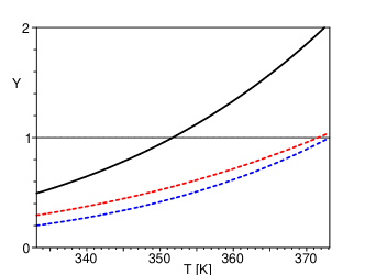
Figure 7: Relative number densities $Y=n^{(0)}/n_{0}$ of saturated vapour of water (blue dashed line) and n-heptane (red dashed line) and their sum are plotted vs. temperature; $Y(T)$ are calculated with Eq. (94).

D.2 Transport coefficients $D_{12}(T_{\ast})$ and $\eta_{12}(T_{\ast})$

For evaluation of the transport coefficients of the vapour mixture the Chapman–Enskog kinetic theory of non-uniform gases Chapman-Cowling-1970 can be employed. The first Chapman–Enskog approximation for the diffusion coefficient $D_{12}$ is independent of the component concentration;

$$D_{12}=\frac{3}{8n_{0}d_{12}^{2}}\sqrt{\frac{k_{\mathrm{B}}T}{2\pi}\left(\frac{1}{m_{1}}+\frac{1}{m_{2}}\right)}\,,\quad n_{0}=\frac{P_{0}}{k_{\mathrm{B}}T}\,.$$ (96)

Here $m_{j}$ is the molecule mass; $\pi d_{12}^{2}$ is the scattering cross section (for an elastic sphere gas, $d_{j}$ is the sphere diameter), with a good accuracy $d_{12}=(d_{1}+d_{2})/2$, where $\pi d_{j}^{2}$ is the scattering cross section for mutual collisions of the molecules of sort $j$.

According to Wilke Wilke-1950 , the ideal gas mixture viscosity can be quite accurately calculated as

$$\eta_{12}\approx \frac{\eta_{1}}{\displaystyle 1+\frac{(n_{2}/n_{1})[1+(\eta_{1}/\eta_{2})^{1/2}(m_{2}/m_{1})^{1/4}]^{2}}{(4/\sqrt{2})[1+(m_{1}/m_{2})]^{1/2}}}$$

$$+\frac{\eta_{2}}{\displaystyle 1+\frac{(n_{1}/n_{2})[1+(\eta_{2}/\eta_{1})^{1/2}(m_{1}/m_{2})^{1/4}]^{2}}{(4/\sqrt{2})[1+(m_{2}/m_{1})]^{1/2}}}\,,$$ (97)

where $\eta_{j}$ is the dynamic viscosity of the pure gas of specie $j$ at atmospheric pressure. At temperature $T_{\ast}$, $n_{j}=n_{j}^{(0)}$. The dynamic viscosity of single component gas can be calculated with the Chapman–Enskog theory; to the forth order Chapman-Cowling-1970 ,

$$\eta_{j}=1.02513\frac{5}{16}\frac{\sqrt{m_{j}k_{\mathrm{B}}T}}{\pi^{1/2}d_{j}^{2}\Omega_{\eta}(k_{\mathrm{B}}T/\varepsilon_{12})}\,,$$ (98)

where geometric factor $\Omega_{\eta}$ is of order of $1$ and characterises interparticle interactions during collisions (e.g., for an elastic sphere gas, $\Omega_{\eta}=1$), $\varepsilon_{12}$ is a reference value of the intermolecular interaction energy.

With Eqs. (96)–(98) and molecular parameters from Tab. 2, one can calculate for the n-heptane–water vapour mixture at $T=T_{\ast}$ ($n_{j}=n_{j\ast}^{(0)}$ were calculated in the previous subsection): $D_{12}(T_{\ast})=1.20\cdot 10^{-5}\mathrm{m^{2}/s}$ and $\eta_{12}(T_{\ast})=0.59\cdot 10^{-5}\mathrm{Pa\cdot s}$.

References

- (1) E. Krell, Handbook of Laboratory Distillation, 2nd ed. (Elsevier, 1982), Chapter 4.3.
- (2) C. J. Geankoplis, Transport Processes and Separation Process Principles, 4th ed. (Prentice Hall, 2003).
- (3) H. C. Simpson, G. C. Beggs, M. Nazir, Evaporation Of Butane Drops In Brine, Desalination 15, 11 (1974).
- (4) G. P. Celata, M. Cumo, F. D’Annibale, F. Gugliermetti, G. Ingui’, Direct contact evaporation of nearly saturated R 114 in water, Int. J. Heat Mass Transfer 38, 1495 (1995).
- (5) M. L. Roesle, F. A. Kulacki, An experimental study of boiling in dilute emulsions, part A: heat transfer, Int. J. Heat Mass Transfer 55, 2160 (2012).
- (6) M. L. Roesle, F. A. Kulacki, An experimental study of boiling in dilute emulsions, part B: visualization, Int. J. Heat Mass Transfer, 55, 2166 (2012).
- (7) S. Sideman, J. Isenberg, Direct Contact Heat Transfer with Change of Phase: Bubble Growth in Three-Phase Systems, Desalination 2, 207 (1967).
- (8) A. A. Kendoush, Theory of convective drop evaporation in direct contact with an immiscible liquid, Desalination 169, 33 (2004).
- (9) A. V. Pimenova, D. S. Goldobin, Boiling at the Boundary of Two Immiscible Liquids below the Bulk Boiling Temperature of Each Component, JETP 119(1), 91 (2014).
- (10) F. P. Incropera, D. P. DeWitt, T. L. Bergman, A. S. Lavine, Fundamentals of Heat and Mass Transfer (John Wiley & Sons, 2006).
-
(11)
D. S. Goldobin, K. G. Kostarev, A. I. Mizev, A. V. Shmyrov,
Combustion of n-heptane layer over water – direct contact
boiling,
http://www.youtube.com/watch?v=UK4FYteCnUE. - (12) S. I. Anisimov, A. Kh. Rakhmatulina, The dynamics of the expansion of a vapor when evaporated into a vacuum, Sov. Phys. JETP 37, 441 (1973).
- (13) G. Filipczak, L. Troniewski, S. Witczak, in Evaporation, Condensation and Heat transfer, Ed. by A. Ahsan (InTech, 2011).
- (14) K. F. Gordon, T. Singh, E. Y. Weissman, Boiling heat transfer between immiscible liquids, Int. J. Heat and Mass Transfer 3, 90 (1961).
- (15) C. B. Prakash, K. L. Pinder, Direct contact heat transfer between two immiscible liquids during vaporisation, Can. J. Chem. Engineering 45, 210 (1967).
- (16) C. B. Prakash, K. L. Pinder, Direct contact heat transfer between two immiscible liquids during vaporization: Part II: Total evaporation time, Can. J. Chem. Engineering 45, 215 (1967).
- (17) T. G. Somer, M. Bora, O. Kaymakcalan, S. Ozmen, Y. Arikan, Desalination 13, 231 (1973).
- (18) L. P. Pitaevskii, E. M. Lifshitz, Course of Theoretical Physics, Vol. 10: Physical Kinetics (Pergamon Press, 2008).
- (19) L. P. Pitaevskii, E. M. Lifshitz, Course of Theoretical Physics, Vol. 9: Statistical Physics, Part 2. Theory of the Condensed State (Pergamon Press, 1980).
- (20) L. Rayleigh, Investigation of the character of the equilibrium of an incompressible heavy fluid of variable density, Proceedings of the London Mathematical Society, 14, 170 (1883).
- (21) G. Taylor, The instability of liquid surfaces when accelerated in a direction perpendicular to their planes, Proceedings of the Royal Society of London. Series A. Mathematical and Physical Sciences 201(1065), 192 (1950).
- (22) D. H. Sharp, An Overview of Rayleigh-Taylor Instability, Physica D 12, 318 (1984).
- (23) D. S. Goldobin, N. V. Brilliantov, Diffusive counter dispersion of mass in bubbly media, Phys. Rev. E 84, 056328 (2011).
- (24) S. Chapman, T. G. Cowling, The mathematical theory of non-uniform gases (Cambridge University Press, 1970).
- (25) C. R. Wilk, A viscosity equation for gas, J. Chem. Phys. 18(4), 517 (1950).