SLAC–PUB–16008

Bootstrapping six-gluon scattering
in planar ${\cal N}=4$ super-Yang-Mills theory

Lance J. Dixon⁽¹⁾, James M. Drummond^(2,3,4),
Claude Duhr⁽⁵⁾, Matt von Hippel⁽⁶⁾
and Jeffrey Pennington^(1)
(1)SLAC National Accelerator Laboratory, Stanford University, Stanford, CA 94309, USA
⁽²⁾School of Physics & Astronomy, Univ. of Southampton, Highfield, Southampton, SO17 1BJ, U.K.
⁽³⁾CERN, Geneva 23, Switzerland
⁽⁴⁾LAPTH, CNRS et Université de Savoie, F-74941 Annecy-le-Vieux Cedex, France
⁽⁵⁾Institute for Particle Physics Phenomenology, University of Durham, Durham, DH1 3LE, U.K.
⁽⁶⁾Simons Center for Geometry and Physics, Stony Brook University, Stony Brook NY 11794, USA

Abstract

We describe the hexagon function bootstrap for solving for six-gluon scattering amplitudes in the large $N_{c}$ limit of ${\cal N}=4$ super-Yang-Mills theory. In this method, an ansatz for the finite part of these amplitudes is constrained at the level of amplitudes, not integrands, using boundary information. In the near-collinear limit, the dual picture of the amplitudes as Wilson loops leads to an operator product expansion which has been solved using integrability by Basso, Sever and Vieira. Factorization of the amplitudes in the multi-Regge limit provides additional boundary data. This bootstrap has been applied successfully through four loops for the maximally helicity violating (MHV) configuration of gluon helicities, and through three loops for the non-MHV case.

1 Introduction

It has long been a dream to construct relativistic scattering amplitudes in four dimensions directly from their analytic structure [1]. In most theories, there has been insufficient information to carry out this program at the level of integrated amplitudes, although a lot of progress has been made at the level of loop integrands. However, ${\cal N}=4$ super-Yang-Mills theory in the planar limit of a large number of colors is very special. Its perturbative amplitudes appear to have uniform transcendental weight $2L$ for the finite parts at $L$ loops. They also have a dual (super)conformal invariance for any number $n$ of external gluons [2, 3, 4]. This symmetry fixes the form of the four- and five-gluon amplitudes to be equal to the BDS ansatz [5]. It also requires the remainder function [6], which first appears for six gluons, to depend only on a limited number of dual conformally invariant cross ratios.

At strong coupling, amplitudes resemble soap bubbles in that the string world-sheet has minimal area in anti-de Sitter space; the minimal-area prescription is equivalent to computing a polygonal Wilson loop expectation value at strong coupling [3]. This duality between amplitudes and Wilson loops also holds at weak coupling [7]. It implies that the near-collinear limits, in which two gluon momenta are almost parallel, can be evaluated in terms of an operator product expansion (OPE) for the Wilson loop, in terms of the excitations of a flux tube [8, 9, 10]. Remarkably, the OPE problem can be solved exactly in the Yang-Mills coupling using integrability [11, 12, 13, 14]. Also, the multi-Regge limits, in which four outgoing gluons are widely separated in rapidity, have a factorization structure [15, 16, 17, 18, 19, 20, 21, 22, 23] which is ordered logarithmically and allows for the recycling of lower-loop information to higher loops. Finally, the super-Wilson-loop correspondence [24, 25] leads to a set of first-order differential equations [26, 27]. These differential equations determine the full $S$ matrix in principle, given the knowledge of higher-point, lower-loop amplitudes that appear as source terms. They can also be used to infer additional, global constraints on amplitudes with a fixed number of legs.

Perturbative amplitudes in planar ${\cal N}=4$ super-Yang-Mills theory certainly enjoy many other fascinating properties. However, as we will sketch in these proceedings, the three properties just mentioned — the near-collinear limits, the multi-Regge limits, and the constraints from the super-Wilson-loop — are extremely powerful. Together with a specific functional ansatz and some simpler constraints, they uniquely determine the six-gluon MHV amplitude through at least four loops [20, 28, 29], and the six-gluon non-MHV or next-to-MHV (NMHV) amplitude through at least three loops [30, 31].

2 Preliminaries

We work with finite quantities from the very beginning: the remainder function [6] for the MHV amplitude and the ratio function [32] for the NMHV amplitude. In this way, we bypass all subtleties of infrared regularization. The six-gluon remainder function $R_{6}$ is defined from the MHV amplitude by factoring off the BDS ansatz [5],

$$A_{6}^{\rm MHV}(\epsilon;s_{ij})=A_{6}^{\rm BDS}(\epsilon;s_{ij})\times\exp[R_{6}(u,v,w)]\,,$$ (1)

where $s_{ij}=(k_{i}+k_{j})^{2}$ are momentum invariants. This procedure not only removes all infrared divergences (poles in $\epsilon=(4-D)/2$), it also removes a dual conformal anomaly [33] in the full amplitude. The remainder function $R_{6}$ is infrared finite, and depends on just three dual conformal cross ratios, $u$, $v$ and $w$.

The amplitude appearing in eq. (1) is color-ordered. The cyclic ordering of the six external gluons makes it possible to define dual or sector variables $x_{i}$ whose differences are the momenta $k_{i}$: $x_{i,i+1}\equiv x_{i}-x_{i+1}=k_{i}$. The key transformation needed to ensure dual conformal invariance is an inversion of the $x_{i}$:

$$x_{i}^{\mu}\to\frac{x_{i}^{\mu}}{x_{i}^{2}}\,,\qquad x_{ij}^{2}\to\frac{x_{ij}^{2}}{x_{i}^{2}\,x_{j}^{2}}\,.$$ (2)

This transformation leaves invariant the dual conformal cross ratios defined by

$$u_{ijkl}=\frac{x_{ij}^{2}\,x_{kl}^{2}}{x_{ik}^{2}\,x_{jl}^{2}}\,.$$ (3)

Because the external momenta are massless, the differences of adjacent $x_{i}$’s have vanishing invariants, $x_{i,i+1}^{2}=k_{i}^{2}=0$. Consequently, there are no dual conformal cross ratios for four or five external gluons.

For the six-gluon case there are just three possible cross ratios, which are related to each other by cyclic permutations:

$$u=\frac{x_{13}^{2}\,x_{46}^{2}}{x_{14}^{2}\,x_{36}^{2}}\,,\qquad v=\frac{x_{24}^{2}\,x_{51}^{2}}{x_{25}^{2}\,x_{41}^{2}}\,,\qquad w=\frac{x_{35}^{2}\,x_{62}^{2}}{x_{36}^{2}\,x_{52}^{2}}\,.$$ (4)

The variables $(u,v,w)$ provide the arguments for $R_{6}$ in eq. (1). Fig. 1 shows the space $(u,v,w)$, along with some distinguished limiting regions. The amplitude is real on a Euclidean sheet in the positive octant with $u>0$, $v>0$ and $w>0$.

The near-collinear limit in which gluons 2 and 3 become parallel, $x_{24}^{2}=(k_{2}+k_{3})^{2}\to 0$, sends $v\to 0$ and also constrains $u+w$ to be 1. It is shown as the solid green line in the figure. There are two other limits, related by cyclic symmetry, shown as dashed green lines. The near-collinear limit can be taken on the Euclidean sheet. The multi-Regge limit for $2\rightarrow 4$ scattering is obtained by first moving onto a Minkowski sheet by taking $u\to e^{-2\pi i}u$. Then one approaches the black point in the figure, $(u,v,w)\to(1,0,0)$, by taking $u\to 1$ and $v,w\to 0$ with the ratios $v/(1-u)$ and $w/(1-u)$ held fixed. These two limits provide the main physical constraints we impose on the amplitude. The analytic expressions for the amplitudes simplify somewhat on the red line $(1,v,v)$ and on the purple line $(u,u,u)$. They reduce further, to linear combinations of multiple zeta values (MZVs), at the intersection of these lines at the point $(u,v,w)=(1,1,1)$.

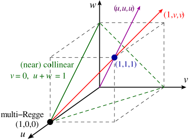
Figure 1: Space of cross ratios $(u,v,w)$ for six-gluon scattering. Various limits are described in the text.

3 Hexagon Functions

We can expand the remainder function perturbatively,

$$R_{6}(u,v,w)=\sum_{L=2}^{\infty}a^{L}\,R_{6}^{(L)}(u,v,w),$$ (5)

where $a=g_{\rm YM}^{2}N_{c}/(8\pi^{2})$ is the ’t Hooft coupling constant, $g_{\rm YM}$ is the Yang-Mills coupling constant and $N_{c}$ is the number of colors. The remainder function begins at two loops [6]. Taking inspiration from the simplified analytic form of the two-loop result [34], we assume [20, 28] that the $L$-loop remainder function $R_{6}^{(L)}$ is a linear combination of weight-$2L$ hexagon functions (to be defined shortly).

The NMHV amplitude really consists of many different components, related to each other by ${\cal N}=4$ supersymmetry. It is best described using an on-shell superspace [35] and defining the ratio of the NMHV superamplitude to the MHV superamplitude [4],

$${\cal P}^{\rm NMHV}\equiv\frac{{\cal A}^{\rm NMHV}}{{\cal A}^{\rm MHV}}\,,$$ (6)

We assume [30] that this super-ratio can be expressed as

$${\cal P}^{\rm NMHV} = \frac{1}{2}\Bigl{[}[(1)+(4)]V(u,v,w)+[(2)+(5)]V(v,w,u)+[(3)+(6)]V(w,u,v)$$ (8)

$$\hskip 0.0pt+[(1)-(4)]\tilde{V}(u,v,w)-[(2)-(5)]\tilde{V}(v,w,u)+[(3)-(6)]\tilde{V}(w,u,v)\Bigr{]}\,,$$

where $(1)\equiv[23456]$ is a shorthand for a certain five-bracket dual superconformal $R$-invariant, and where the $L$-loop coefficients in the perturbative expansions of $V$ and $\tilde{V}$,

$$V(u,v,w) = \sum_{L=0}^{\infty}a^{L}\,V^{(L)}(u,v,w),$$ (9)

$$\tilde{V}(u,v,w) = \sum_{L=2}^{\infty}a^{L}\,\tilde{V}^{(L)}(u,v,w),$$ (10)

are also weight-$2L$ hexagon functions.

Hexagon functions form a certain class of iterated integrals [36] or multiple polylogarithms [37, 38]. If we differentiate a weight-$n$ function $f$ in this class, the result can be written as

$$df=\sum_{s_{k}\in{\cal S}}f^{s_{k}}\,d\ln s_{k}\,,$$ (11)

where ${\cal S}$ is a finite set of rational expressions, known as the letters of the symbol, and $f^{s_{k}}$ are weight-$(n-1)$ functions in the same class. These functions describe the $\{n-1,1\}$ component of a coproduct $\Delta$ associated with a Hopf algebra for iterated integrals [39, 40, 41]. Similarly, we can differentiate each $f^{s_{k}}$,

$$df^{s_{k}}=\sum_{s_{j}\in{\cal S}}f^{s_{j}\,s_{k}}\,d\ln s_{j}\,,$$ (12)

thereby defining the weight-$(n-2)$ functions $f^{s_{j}\,s_{k}}$, which describe the $\{n-2,1,1\}$ components of $\Delta$. The maximal iteration of this procedure defines the symbol of $f$, an $n$-fold tensor product of elements of ${\cal S}$ (each standing for a $d\ln$).

Hexagon functions are functions whose symbols have letters drawn from the nine-letter set,

$${\cal S}=\{u,v,w,1-u,1-v,1-w,y_{u},y_{v},y_{w}\}\,.$$ (13)

The nine letters can be understood to arise from momentum twistors [42] $Z_{i}^{A}$, $i=1,2,\ldots,6$, $A=1,2,3,4$, because these objects transform simply under dual conformal transformations, as do the four-brackets $\langle ijkl\rangle\equiv\varepsilon_{ABCD}Z_{i}^{A}Z_{j}^{B}Z_{k}^{C}Z_{l}^{D}$. However, the four-brackets are not invariant under projective transformations (rescalings). There are 15 projectively invariant ratios of four-brackets, and they can be factored into the nine basic ones, given in eq. (13). The three variables $y_{u}$, $y_{v}$, $y_{w}$ are not independent of $u,v,w$ but satisfy

$$y_{u}=\frac{u-z_{+}}{u-z_{-}}\,,\qquad y_{v}=\frac{v-z_{+}}{v-z_{-}}\,,\qquad y_{w}=\frac{w-z_{+}}{w-z_{-}}\,,$$ (14)

where

$$z_{\pm}=\frac{1}{2}\Bigl{[}-1+u+v+w\pm\sqrt{\Delta}\Bigr{]}\,,\qquad\Delta=(1-u-v-w)^{2}-4uvw\,.$$ (15)

Although $y_{u},y_{v},y_{w}$ contain square roots when expressed in terms of $u,v,w$, the converse is not true; $u$ is given by the rational expression,

$$u=\frac{y_{u}(1-y_{v})(1-y_{w})}{(1-y_{u}y_{v})(1-y_{u}y_{w})}\,,$$ (16)

and $v$ and $w$ are given by cyclic permutations of this relation.

Hexagon functions have one other defining property: Their branch cuts should start only at the origin in the momentum invariants $(k_{i}+k_{i+1})^{2}$ and $(k_{i}+k_{i+1}+k_{i+2})^{2}$, which means they should start only at 0 or $\infty$ in the cross ratios $u,v,w$. In terms of the symbol, the first entry must be drawn from $\{u,v,w\}$ [10].

In certain regions, hexagon functions collapse to simpler functions. For example:

1. On the lines $(u,u,1)$ and $(u,1,1)$, the set ${\cal S}$ collapses to $\{u,1-u\}$, corresponding to the harmonic polylogarithms (HPLs) defined by Remiddi and Vermaseren [43], with weight vectors $0$ and $1$ only.

2. On the line $(u,u,u)$, ${\cal S}$ collapses to $\{y_{u},1+y_{u},1+y_{u}+y_{u}^{2}\}$, corresponding to cyclotomic polylogarithms [44], because $1+y_{u}$ and $1+y_{u}+y_{u}^{2}$ vanish when $y_{u}$ is a sixth root of unity.

3. In the multi-Regge limit, with $v/(1-u)=1/[(1-z)(1-\bar{z})]$, $w/(1-u)=z\bar{z}/[(1-z)(1-\bar{z})]$, the relevant functions [23] have symbol letters $\{z,1-z,\bar{z},1-\bar{z}\}$, plus a first-entry or single-valuedness constraint. These single-valued harmonic polylogarithms (SVHPLs) have been studied by Brown [45].

Two complementary methods have been used to construct hexagon functions [28, 29]. One approach is to represent each hexagon function in terms of multiple polylogarithms in the $y_{i}$ variables, for a particular region in the space of cross ratios. The multiple polylogarithms can be evaluated numerically using GiNaC [46, 47]. They can also be expanded analytically in various limits as needed to impose physical constraints. Alternatively, one can define the hexagon functions iteratively via the $\{n-1,1\}$ components of their coproducts, which amount to a set of coupled first-order differential equations. These equations can be integrated numerically, or solved analytically in special limits, such as the ones enumerated above.

The complete set of hexagon functions through weight five has been described using both methods [28]. This set suffices to characterize the weight-six three-loop functions $R_{6}^{(3)}$, $V^{(3)}$ and $\tilde{V}^{(3)}$ via their weight-five $\{5,1\}$ coproduct components, i.e. their first derivatives, up to constants of integration which can also be fixed. To go to four loops, one can start by enumerating the possible $\{5,1,1,1\}$ coproduct components, and then work upward, through the $\{6,1,1\}$ and $\{7,1\}$ components, in order to characterize the full space of weight-eight functions. Some mathematical consistency conditions have to be imposed throughout the construction, namely the equality of mixed partial derivatives, and the absence of branch cuts in undesired locations.

4 Applying constraints

Once one understands the space of functions, the basic strategy of the hexagon function bootstrap at $L$ loops is very simple:

1. Enumerate all the hexagon functions at weight $2L$. This list contains products of lower-weight functions, such as the products of weight-$k$ MZVs (constants) with weight-$(2L-k)$ hexagon functions.

2. Write the most general linear combination of such functions with unknown rational-number coefficients.

3. Impose certain symmetry properties and other simple constraints, followed by the super-Wilson-loop, OPE and multi-Regge constraints, until all coefficients have been uniquely determined.

Sometimes we perform the last step in two stages. In the first stage, we fix the symbol of the desired function. In the second stage, we determine the full function, including some Riemann $\zeta$-valued ambiguities present at symbol level.

The simple constraints on $R_{6}$ are:

1. Total symmetry under exchange of $u,v,w$.

2. Even under “parity” ($y_{i}\leftrightarrow 1/y_{i}$); every term in its symbol must contain an even number of $y_{i}$.

3. Vanishing in the collinear limit, $R_{6}\to 0$ as $v\to 0$, $u+w\to 1$.

4. Final entry restricted [27] to six combinations: $\{u/(1-u),v/(1-v),w/(1-w),y_{u},y_{v},y_{w}\}$.

The simple constraints on $V(u,v,w)$ ($\tilde{V}(u,v,w)$) are:

1. Symmetric (antisymmetric) under exchange of $u$ and $w$.

2. Even (odd) under “parity”.

3. Cancellation of spurious poles arising from the prefactors $(i)$.

4. Collinear vanishing.

5. Final entry restricted [27, 48] to seven combinations, where the extra combination is $uw/v$.

The spurious-pole and collinear constraints on the ratio function involve a couple of different permutations of $V$ and $\tilde{V}$ [30].

The OPE constraints are imposed in the limit $\tau\to\infty$, where $v\approx T^{2}\to 0$, $T\equiv e^{-\tau}$. The other relevant variables in this limit are $\sigma\approx\frac{1}{2}\ln(u/w)$, which characterizes the longitudinal splitting fraction of the two collinear gluons; and $\phi$, which is an azimuthal angle. The original OPE constraints [8, 9, 10] only fixed the “leading discontinuity” terms, which for the remainder function have the form $(\ln T)^{L-1}$. The new integrability-based results give all powers of $\ln T$ for the leading power-law (leading twist) behavior coming from a single flux-tube excitation [11, 12]. These terms have the form $Te^{\pm i\phi}(\ln T)^{k}f_{k}(\sigma)$, $k=0,1,2,\ldots,L-1$, for some functions $f_{k}(\sigma)$ involving HPLs. More recently, the two-excitation contributions have also become available [13]; they behave like $T^{2}\{e^{\pm 2i\phi},1\}(\ln T)^{k}f_{k}(\sigma)$, $k=0,1,2,\ldots,L-1$. The $\phi$ dependence is controlled by the angular momentum of the excitations. At leading twist, only gluons (spin $\pm 1$) contribute. At the next order, pairs of fermions and scalars can also contribute, to the 1 term but not to the $e^{\pm 2i\phi}$ terms, which are purely gluonic. The gluonic terms can be controlled to arbitrary order in $T$ [14].

The imposition of the multi-Regge constraints is described elsewhere [20, 23, 28, 29, 31].

In the case of the remainder function, we fixed the symbol first. Table 1 summarizes how many unknown parameters are left after each constraint is imposed. There are also parameters multiplying Riemann $\zeta$ values, to which the symbol is insensitive. At four loops, for example, there are 68 such parameters [29]. They can be fixed by imposing the same constraints at function level. For the $T^{2}$ OPE constraints, only the $T^{2}\cdot e^{\pm 2i\phi}$ terms had to be imposed to fix everything. The $T^{2}\cdot 1$ terms provided a pure cross check.

Constraint	$L=2$	$L=3$	$L=4$
1. Integrability	75	643	5897
2. Total $S_{3}$ symmetry	20	151	1224
3. Parity invariance	18	120	874
4. Collinear vanishing ($T^{0}$)	4	59	622
5. OPE leading discontinuity	0	26	482
6. Final entry	0	2	113
7. Multi-Regge limit	0	2	80
8. Near-collinear OPE ($T^{1}$)	0	0	4
9. Near-collinear OPE ($T^{2}$)	0	0	0

Table 1: Remaining parameters in the symbol of $R_{6}^{(L)}$ at loop order $L=2,3,4$, after applying the various constraints successively [29]. Once a “0” appears, the symbol is uniquely determined. Further 0’s represent cross checks from additional constraints.

For the ratio function, we imposed the constraints at the function level from the beginning. The number of parameters remaining in this case is shown in table 2. The cyclic vanishing constraint on $\tilde{V}$ is required because of an identity obeyed by the $(i)$ invariants, $[(1)+(3)+(5)]-[(2)+(4)+(6)]=0$. For details on how the remaining constraints were imposed, see refs. [30, 31]. Either the $T^{2}$ OPE or the multi-Regge constraints were sufficient to fix the last two parameters, leaving the other set of constraints as a pure cross check.

Constraint	$L=1$	$L=2$	$L=3$
1. (Anti)symmetry in $u$ and $w$	7	52	412
2. Cyclic vanishing of $\tilde{V}$	7	52	402
3. Final-entry condition	4	25	182
4. Spurious-pole vanishing	3	15	142
5. Collinear vanishing	1	8	92
6. ${\cal O}(T^{1})$ OPE	0	0	2
7. ${\cal O}(T^{2})$ OPE or multi-Regge kinematics	0	0	0

Table 2: Remaining parameters in the function-level ansätze for $V^{(L)}$ and $\tilde{V}^{(L)}$ after each constraint is applied, at each loop order [31].

5 Results

Having determined the functions $R_{6}$, $V$ and $\tilde{V}$, we can plot them, and examine some of their analytic properties. At the point $(u,v,w)=(1,1,1)$, hexagon functions all collapse to MZVs. For the remainder function we find,

$$R_{6}^{(2)}(1,1,1) = -(\zeta_{2})^{2}=-\frac{5}{2}\zeta_{4}\,,$$ (17)

$$R_{6}^{(3)}(1,1,1) = \frac{413}{24}\,\zeta_{6}+(\zeta_{3})^{2}\,,$$ (18)

$$R_{6}^{(4)}(1,1,1) = -\frac{3}{2}\zeta_{2}(\zeta_{3})^{2}-\frac{5}{2}\zeta_{3}\zeta_{5}-\frac{471}{4}\zeta_{8}+\frac{3}{2}\zeta_{5,3}\,.$$ (19)

The first MZV that is irreducible (cannot be written in terms of $\zeta_{k}$’s) occurs at weight eight; this quantity, $\zeta_{5,3}$, does appear in $R_{6}^{(4)}(1,1,1)$.

An interesting line on which to plot the remainder function is when all three cross ratios are equal, i.e. the line $(u,u,u)$. Fig. 2 shows the two-, three-, four-loop and strong-coupling remainder functions on this line. The strong-coupling result is computed from the minimal-area prescription [3, 49]. The plots are not partial sums — that would require us to choose a value for the ’t Hooft coupling — but rather the individual coefficient functions. We have rescaled them all by their values at $u=1$. Remarkably, for $u<1$, all four curves have very similar shapes, even though they are composed of quite different analytic functions — cyclotomic polylogarithms [44] of different weights at weak coupling, and an arccosine at strong coupling [49]. This remarkable similarity in shape was noticed already at two loops [51]. It clearly persists through four loops for $u<1$. More generally, ratios of successive loop orders for the remainder function tend to vary quite slowly with $u,v,w$, at least within the unit cube and when $u,v,w$ are not too small.

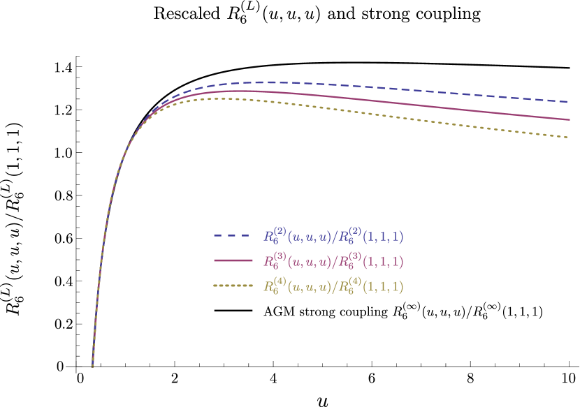
Figure 2: The remainder function on the line $(u,u,u)$, plotted at two, three, and four loops and at strong coupling, after normalizing the coefficient functions by their values at the point $(1,1,1)$ [29].

Finally, in fig. 3 we plot the three-loop remainder function $R_{6}^{(3)}(u,v,w)$ and ratio function components $V^{(3)}(u,v,w)$ and $\tilde{V}^{(3)}(u,v,w)$ on the triangle which is the part of the plane $u+v+w=1$ that lies in the positive octant. The remainder function is constrained to vanish on all three edges of the triangle (the collinear limits); consequently it never gets very large in the interior. For the ratio function, the collinear-vanishing constraint involves a linear combination of two permutations of $V$, and so $V^{(3)}$ does not have to vanish on the edges. ($\tilde{V}^{(3)}$, like all parity-odd hexagon functions, actually does vanish on the edges, but the vanishing happens so slowly that it is not visible in the plots.)

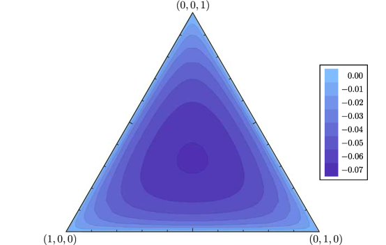
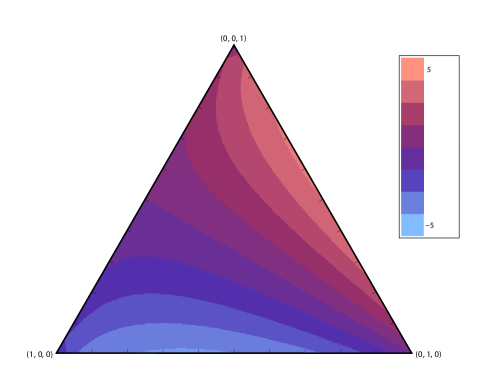
Figure 3: The three-loop functions $R_{6}^{(3)}$, $V^{(3)}$ and $\tilde{V}^{(3)}/i$, plotted on the plane $u+v+w=1$ [28, 31].

6 Conclusions

Scattering amplitudes in planar ${\cal N}=4$ super-Yang-Mills theory are so strongly constrained that it is feasible to compute them using a bootstrap that operates at the level of integrated amplitudes, without any direct knowledge of the integrands at high loop orders. We have demonstrated the practicality of this bootstrap for the six-gluon scattering amplitude, for both the MHV and NMHV helicity configurations. Of course, some notion of the space in which the solution lies is necessary. In the six-gluon case it is provided by hexagon functions, motivated by the simple form found earlier for the two-loop remainder function. The existence of detailed boundary value “data” from the near-collinear and multi-Regge limits was also essential. The numerical and analytic results obtained so far exhibit interesting patterns, which may help in constructing all-orders solutions. It would be very interesting to try to extend these methods to other amplitudes in planar ${\cal N}=4$ super-Yang-Mills theory, and to more general theories as well.

Acknowledgments This research was supported by the US Department of Energy under contracts DE–AC02–76SF00515 and DE–FG02–92ER40697, by the Research Executive Agency (REA) of the European Union under the Grant Agreement PITN-GA-2010-264564 (LHCPhenoNet) and by the EU Initial Training Network in High-Energy Physics and Mathematics: GATIS. LD is grateful to the organizers of Loops and Legs for the opportunity to present this work at such a stimulating meeting, and to the Simons Center for Geometry and Physics for hospitality when some of this research was performed.

References

- [1] R. J. Eden, P. V. Landshoff, D. I. Olive, J. C. Polkinghorne, “The Analytic -Matrix”, Cambridge University Press (1966).
-
[2]
J. M. Drummond, J. Henn, V. A. Smirnov and E. Sokatchev,
JHEP 0701 (2007) 064
[hep-th/0607160];
Z. Bern, M. Czakon, L. J. Dixon, D. A. Kosower and V. A. Smirnov, Phys. Rev. D 75 (2007) 085010 [hep-th/0610248];
Z. Bern, J. J. M. Carrasco, H. Johansson and D. A. Kosower, Phys. Rev. D 76 (2007) 125020 [arXiv:0705.1864 [hep-th]]. - [3] L. F. Alday and J. M. Maldacena, JHEP 0706 (2007) 064 [arXiv:0705.0303 [hep-th]].
- [4] J. M. Drummond, J. Henn, G. P. Korchemsky and E. Sokatchev, Nucl. Phys. B 828 (2010) 317 [arXiv:0807.1095 [hep-th]].
- [5] Z. Bern, L. J. Dixon and V. A. Smirnov, Phys. Rev. D 72, 085001 (2005) [hep-th/0505205].
-
[6]
Z. Bern, L. J. Dixon, D. A. Kosower, R. Roiban, M. Spradlin,
C. Vergu and A. Volovich,
Phys. Rev. D 78 (2008) 045007
[arXiv:0803.1465 [hep-th]];
J. M. Drummond, J. Henn, G. P. Korchemsky and E. Sokatchev, Nucl. Phys. B 815 (2009) 142 [arXiv:0803.1466 [hep-th]]. -
[7]
J. M. Drummond, G. P. Korchemsky and E. Sokatchev,
Nucl. Phys. B 795 (2008) 385
[arXiv:0707.0243 [hep-th]];
A. Brandhuber, P. Heslop and G. Travaglini, Nucl. Phys. B 794 (2008) 231 [arXiv:0707.1153 [hep-th]]. - [8] L. F. Alday, D. Gaiotto, J. Maldacena, A. Sever and P. Vieira, JHEP 1104 (2011) 088 [arXiv:1006.2788 [hep-th]].
- [9] D. Gaiotto, J. Maldacena, A. Sever and P. Vieira, JHEP 1103 (2011) 092 [arXiv:1010.5009 [hep-th]].
- [10] D. Gaiotto, J. Maldacena, A. Sever and P. Vieira, JHEP 1112 (2011) 011 [arXiv:1102.0062 [hep-th]].
- [11] B. Basso, A. Sever and P. Vieira, Phys. Rev. Lett. 111, 091602 (2013) [arXiv:1303.1396 [hep-th]].
- [12] B. Basso, A. Sever and P. Vieira, JHEP 1401, 008 (2014) [arXiv:1306.2058 [hep-th]].
- [13] B. Basso, A. Sever and P. Vieira, arXiv:1402.3307 [hep-th].
- [14] B. Basso, A. Sever and P. Vieira, arXiv:1407.1736 [hep-th].
- [15] J. Bartels, L. N. Lipatov and A. Sabio Vera, Phys. Rev. D 80 (2009) 045002 [arXiv:0802.2065 [hep-th]].
- [16] J. Bartels, L. N. Lipatov and A. Sabio Vera, Eur. Phys. J. C 65 (2010) 587 [arXiv:0807.0894 [hep-th]].
- [17] L. N. Lipatov and A. Prygarin, Phys. Rev. D 83 (2011) 045020 [arXiv:1008.1016 [hep-th]].
- [18] L. N. Lipatov and A. Prygarin, Phys. Rev. D 83 (2011) 125001 [arXiv:1011.2673 [hep-th]].
- [19] J. Bartels, L. N. Lipatov and A. Prygarin, Phys. Lett. B 705 (2011) 507 [arXiv:1012.3178 [hep-th]].
- [20] L. J. Dixon, J. M. Drummond and J. M. Henn, JHEP 1111 (2011) 023 [arXiv:1108.4461 [hep-th]].
- [21] V. S. Fadin and L. N. Lipatov, Phys. Lett. B 706 (2012) 470 [arXiv:1111.0782 [hep-th]].
- [22] L. Lipatov, A. Prygarin and H. J. Schnitzer, JHEP 1301, 068 (2013) [arXiv:1205.0186 [hep-th]].
- [23] L. J. Dixon, C. Duhr and J. Pennington, JHEP 1210, 074 (2012) [arXiv:1207.0186 [hep-th]].
- [24] L. J. Mason and D. Skinner, JHEP 1012, 018 (2010) [arXiv:1009.2225 [hep-th]].
- [25] S. Caron-Huot, JHEP 1107, 058 (2011) [arXiv:1010.1167 [hep-th]].
- [26] M. Bullimore and D. Skinner, [arXiv:1112.1056 [hep-th]].
- [27] S. Caron-Huot and S. He, JHEP 1207 (2012) 174 [arXiv:1112.1060 [hep-th]].
- [28] L. J. Dixon, J. M. Drummond, M. von Hippel and J. Pennington, JHEP 1312, 049 (2013) [arXiv:1308.2276 [hep-th]].
- [29] L. J. Dixon, J. M. Drummond, C. Duhr and J. Pennington, JHEP 1406, 116 (2014) [arXiv:1402.3300 [hep-th]].
- [30] L. J. Dixon, J. M. Drummond and J. M. Henn, JHEP 1201 (2012) 024 [arXiv:1111.1704 [hep-th]].
- [31] L. J. Dixon and M. von Hippel, to appear.
- [32] J. M. Drummond, J. Henn, G. P. Korchemsky and E. Sokatchev, Nucl. Phys. B 828, 317 (2010) [arXiv:0807.1095 [hep-th]].
- [33] J. M. Drummond, J. Henn, G. P. Korchemsky and E. Sokatchev, Nucl. Phys. B 826, 337 (2010) [arXiv:0712.1223 [hep-th]].
- [34] A. B. Goncharov, M. Spradlin, C. Vergu and A. Volovich, Phys. Rev. Lett. 105 (2010) 151605 [arXiv:1006.5703 [hep-th]].
- [35] V. P. Nair, Phys. Lett. B 214, 215 (1988).
- [36] K. T. Chen, Bull. Amer. Math. Soc. 83, 831 (1977).
- [37] F. C. S. Brown, Annales scientifiques de l’ENS 42, fascicule 3, 371 (2009) [math/0606419].
- [38] A. B. Goncharov, [arXiv:0908.2238v3 [math.AG]].
- [39] A. B. Goncharov, [math/0103059].
- [40] A. B. Goncharov, Duke Math. J. Volume 128, Number 2 (2005) 209.
- [41] F. C. S. Brown, [arXiv:1102.1310 [math.NT]]; [arXiv:1102.1312 [math.AG]].
- [42] A. Hodges, JHEP 1305, 135 (2013) [arXiv:0905.1473 [hep-th]].
- [43] E. Remiddi and J. A. M. Vermaseren, Int. J. Mod. Phys. A 15, 725 (2000) [hep-ph/9905237].
- [44] J. Ablinger, J. Blümlein and C. Schneider, J. Math. Phys. 52 (2011) 102301 [arXiv:1105.6063 [math-ph]].
- [45] F. C. S. Brown, C. R. Acad. Sci. Paris, Ser. I 338 (2004) 527.
- [46] C. W. Bauer, A. Frink and R. Kreckel, [cs/0004015 [cs-sc]].
- [47] J. Vollinga and S. Weinzierl, Comput. Phys. Commun. 167 (2005) 177 [hep-ph/0410259].
- [48] S. Caron-Huot, private communication.
- [49] L. F. Alday, D. Gaiotto and J. Maldacena, JHEP 1109, 032 (2011) [arXiv:0911.4708 [hep-th]].
- [50] B. Basso, A. Sever and P. Vieira, arXiv:1405.6350 [hep-th].
- [51] Y. Hatsuda, K. Ito and Y. Satoh, JHEP 1302, 067 (2013) [arXiv:1211.6225 [hep-th]].
- [52] A. Brandhuber, P. Heslop, V. V. Khoze and G. Travaglini, JHEP 1001, 050 (2010) [arXiv:0910.4898 [hep-th]].
- [53] V. Del Duca, C. Duhr and V. A. Smirnov, JHEP 1009, 015 (2010) [arXiv:1006.4127 [hep-th]].
-
[54]
Y. Hatsuda, K. Ito, K. Sakai and Y. Satoh,
JHEP 1104, 100 (2011)
[arXiv:1102.2477 [hep-th]];
Y. Hatsuda, K. Ito and Y. Satoh, JHEP 1202, 003 (2012) [arXiv:1109.5564 [hep-th]].