Photon-photon correlation statistics in the collective emission from ensembles of self-assembled quantum dots

Abstract

We present a theoretical analysis of the intensity autocorrelation for the spontaneous emission from a planar ensemble of self-assembled quantum dots. Using the quantum jump approach, we numerically simulate the evolution of the system and construct photon-photon delay time statistics that approximates the second order correlation function of the field. The form of this correlation function in the case of collective emission from a highly homogeneous ensemble qualitatively differs form that characterizing an ensemble of independent emitters (inhomogeneous ensemble of uncoupled dots). The signatures of collective emission in the intensity correlations are observed also in the case of an inhomogeneous but sufficiently strongly coupled ensemble. Thus, we show that the second order correlation function of the emitted field provides a sensitive test of cooperative effects.

I Introduction

While the essential luminescence properties of quantum dots (QDs) are determined by single-QD characteristics, the observed enhanced luminescence of QD arrays and ensembles scheibner07 ; mazur09 ; mazur10b reveals physical effects beyond this single emitter picture. Such an enhancement is attributed to collective (cooperative) effects in emission, that is, the quantum-optical phenomenon that leads to markedly non-exponential, peaked emission in atomic samples skribanovitz73 . An obvious difference between the QDs (“artificial atoms”) and the real, natural atoms is the considerable inhomogeneity of optical transition energies in the former case. With a natural emission line width of a single QD on the order of a few $\mu$eV bayer02 , the typical ensemble distribution of transition energies over several to a few tens of meV should preclude any collective emission effects. Theoretical modeling reveals the role of the interplay between this spectral inhomogeneity and the coupling between the QDs sitek07a . By assuming the presence of some kind of electronic couplings (in addition to the fundamental but weak dipole couplings) in the QD ensemble, the experimentally observed enhancement of spontaneous emission in a planar ensemble scheibner07 has been quantitatively reproduced kozub12 . The proposed role of inter-QD couplings is also consistent with the observed cooperative effects in QD chains mazur10b , where the presence of such couplings is much more obvious mazur09 .

The particular dependence of of the enhanced emission rate on the ensemble size, spectral range, and excitation mode is consistent with the concept of its collective nature and strongly supports this interpretation scheibner07 . However, the observed time dependence of the emission intensity for inhomogeneous ensembles of QDs remains exponential scheibner07 ; mazur10b (in contrast to the atomic superradiance) makes this effect purely quantitative and does not allow one to exclude a formally possible conspiracy of different factors that might simply shorten the exciton life time in the QD samples used in the experimental studies. Therefore, one is motivated to look for another characteristics of the emission signal, where the collective effects might be manifested in a more qualitative way. Probably the most obvious option is to look at the second-order correlation function of the emitted radiation, which is experimentally accessible via detection of photon-photon (intensity) correlations and is commonly applied to characterize light fields emitted from QD systems ulrich07 ; Callsen2013 ; Davanco2014 . While the original approach, based on the standard Hanbury-Brown and Twiss setup, limited the temporal resolution of the measured correlation functions to the nanosecond range, the recently developed experimental technique Wiersig2009 ; Assmann2010a ; Assmann2010b gives access to second-order correlations on much shorter time scales. In this method, one uses a streak camera in the single photon counting mode to register the detection traces of incident photons with picosecond resolution. This record of time-labeled photodection events can than be used to determine the statistical properties of a pulse light source with picosecond resolution. Such a procedure has been successfully applied to characterize the light field originating from a QD laser Wiersig2009 ; Assmann2010a .

Theoretical modeling of intensity correlations for QD ensembles focused predominantly on cavity systems ulrich07 . General studies, based on the Master equation approach, revealed strong photon bunching in the emission form a few two-level emitters in cavities below the lasing threshold temnov09 that oscillates with the number of emitters auffeves11 and identified the role of dephasing auffeves11 . For the description of QD systems, the model has been extended to account for multiple excitation of a QD emitter and for the dephasing effects ritter10 , as well as carrier-phonon interaction harsij12 An extended theory has also been proposed ulrich07 ; su10 , based on the cluster expansion, accounting for semiconductor-specific effects, like higher order Coulomb and carrier-photon correlations or Pauli blocking. For free-statnding systems, the intensity correlation has been modeled to characterize two-photon emission from the biexciton cascade from a single QD Callsen2013 .

In this paper, we present a theoretical study of second-order correlations in the pulsed emission from a free-standing (not embedded in a cavity) QD ensemble, using the stochastic simulation (quantum jump) method. This work is motivated by the availability of the experimental technique mentioned above and aims at identifying the signatures of cooperative effects in the emission from such systems, in particular in photon-photon correlations. We study also the dependence of the correlation functions on the energy inhomogeneity and inter-dot couplings in the ensemble. We find out that the form of the second order correlation function in the case of emission from highly homogeneous or sufficiently strongly coupled QD systems qualitatively differs from that characterizing a field generated by an ensemble of independent emitters. Therefore, the second order correlation function of the emitted field provides a sensitive test of cooperative effects in the spontaneous emission.

The paper is organized as follows. Section II defines the model and describes the stochastic simulation method used for the numerical modeling. Sec. III is devoted to simple limitiing cases that can be fully treated analytically. In Sec. IV, we present and discuss the results of the simulations. Section V contains general discussion concluding remarks.

II Model and simulation method

In this section, we first define the model (Sec. II.1), then describe the stochastic method of quantum jumps used to simulate the dynamics (Sec. II.2) and, finally, define the estimates of the correlation functions in terms of the photon emission events yielded by the stochastic simulation (Sec. II.3).

II.1 Model

The system to be modeled consists of a planar, single-layer ensemble of several self-assembled QDs randomly and uniformly placed in the $xy$ plane, as in our earlier work kozub12 . The center-to-center distance between the QDs can not be lower than 10 nm (roughly the QD diameter). The positions of the dots are denoted by $\bm{r}_{\alpha}$, where $\alpha$ numbers the dots. Each QD is modeled as a point-wise two-level system (empty dot and one exciton) with the fundamental transition energy $E_{\alpha}=\overline{E}+\epsilon_{\alpha}$, where $\overline{E}$ is the average transition energy in the ensemble and $\epsilon_{\alpha}$ represent the energy inhomogeneity of the ensemble, described by a Gaussian distribution with zero mean and standard deviation $\sigma$. We assume the dots to be coupled by an interaction $V_{\alpha\beta}$ which is composed of long-range (LR) dipole interaction (dispersion force) and a short-range (SR) coupling (exponentially decaying with the distance),

$$V_{\alpha\beta}=V^{(\mathrm{sr})}_{\alpha\beta}+V^{(\mathrm{lr})}_{\alpha\beta}.$$

The long-range dipole coupling is described by stephen64 ; lehmberg70a ; varfolomeev71 ; kozub12

$$V^{(\mathrm{lr})}_{\alpha\beta}=-\hbar\Gamma_{0}G(k_{0}r_{\alpha\beta}),\quad\alpha\neq\beta,$$

and $V_{\alpha\alpha}=0$, where $\bm{r}_{\alpha\beta}=\bm{r}_{\alpha}-\bm{r}_{\beta}$, $\Gamma_{0}=|d_{0}|^{2}k_{0}^{3}/(3\pi\varepsilon_{0}\varepsilon_{\mathrm{r}})$ is the spontaneous emission (radiative recombination) rate for a single dot, $d_{0}$ is the magnitude of the interband dipole moment (assumed identical for all the dots), $\varepsilon_{0}$ is the vacuum permittivity, $\varepsilon_{\mathrm{r}}$ is the relative dielectric constant of the semiconductor, $k_{0}=n\overline{E}/(\hbar c)$, $c$ is the speed of light, $n=\sqrt{\varepsilon_{\mathrm{r}}}$ is the refractive index of the semiconductor, and, for a heavy-hole transition in a planar ensemble,

$$G(x)=-\frac{3}{8}\left(\frac{\cos x}{x}+\frac{\sin x}{x^{2}}+\frac{\cos x}{x^{3}}\right).$$

The SR coupling is included in accordance with our previous work kozub12 , which suggested its important role in the cooperative emission. Only the overall magnitude and the finite range of this coupling are essentially important, hence we model it by the simple exponential dependence

$$V^{(\mathrm{sr})}_{\alpha\beta}=V_{0}e^{-r_{\alpha\beta}/r_{0}}.$$

The density matrix then evolves according to the Master equationlehmberg70a ; kozub12

$$\dot{\rho}=-\frac{i}{\hbar}[H_{0},\rho]+\sum_{\alpha,\beta=1}^{N}\Gamma_{\alpha\beta}\left[\sigma_{\alpha}\rho\sigma_{\beta}^{{\dagger}}-\frac{1}{2}\left\{\sigma_{\beta}^{{\dagger}}\sigma_{\alpha},\rho\right\}\right].$$ (1)

Here the first term accounts for the unitary evolution of the ensemble of coupled QDs with the Hamiltonian

$$H_{0}=\sum_{\alpha=1}^{N}\epsilon_{\alpha}\sigma_{\alpha}^{\dagger}\sigma_{\alpha}+\sum_{\alpha,\beta=1}^{N}V_{\alpha\beta}\sigma_{\alpha}^{\dagger}\sigma_{\beta},$$ (2)

where we introduce the transition operators for the dots: the “exciton annihilation” operator $\sigma_{\alpha}$, which annihilates an exciton in the dot $\alpha$, and the “exciton creation” operator $\sigma_{\alpha}^{\dagger}$ which creates an exciton in the dot $\alpha$ (the exciton number operator for the dot $\alpha$ is then $\hat{n}_{\alpha}=\sigma_{\alpha}^{{\dagger}}\sigma_{\alpha}$). In Eq. (2), the first term describes the exciton energies in the dots and the second one accounts for the inter-dot coupling. The second term in Eq. (1) describes the dissipation, that is, the collective spontaneous emission process due to the coupling between the quantum emitters (QDs) and their radiative environment (vacuum). Here $\Gamma_{\alpha\alpha}=\Gamma_{0},\quad\Gamma_{\alpha\beta}=\Gamma_{\beta\alpha}=\Gamma_{0}F(k_{0}r_{\alpha\beta})$, with

$$F(x) = \frac{3}{4}\left(\frac{\sin x}{x}-\frac{\cos x}{x^{2}}+\frac{\sin x}{x^{3}}\right),$$

and $\{\ldots,\ldots\}$ denotes the anti-commutator.

The simulations are performed for an ensemble of systems generated by randomly placing a given number of QDs with a fixed surface density $\nu$ in the $xy$ plane and choosing their fundamental transition energies from the Gaussian distribution. We assume the fully inverted initial state corresponding to strong excitation,

$$|\Psi_{0}\rangle=\prod_{\alpha=1}^{N}\sigma_{\alpha}^{{\dagger}}|\mathrm{vac}\rangle,$$

where $|\mathrm{vac}\rangle$ is the “vacuum” state, that is, the crystal ground state state with filled valence band states and empty conduction band states (no excitons in the QDs). Such a state can be created by strong optical excitation. Exciton injection to QD ensembles can also be controlled by an external electric field Baumgartner2010 .

II.2 Stochastic simulation method

We model the evolution of the spontaneous emission process numerically, using the stochastic simulation approach (quantum jump method) Breuer ; Gardiner2004 , which considerably reduces the computational load and allows us to study larger QD ensembles than those tractable by a direct integration of the Master equation. The starting point is Eq. (1) written in the equivalent form

$$\dot{\rho}=-\frac{i}{\hbar}(H_{\mathrm{eff}}\rho-\rho H_{\mathrm{eff}}^{{\dagger}})+\sum_{i=1}^{N}\tilde{\Gamma}_{i}\tilde{\sigma}_{i}\rho\tilde{\sigma}_{i}^{{\dagger}},$$ (3)

where

$$H_{\mathrm{eff}}=H_{0}+\frac{\hbar}{2i}\sum_{\alpha\beta}\Gamma_{\alpha\beta}\sigma_{\beta}^{{\dagger}}\sigma_{\alpha},$$

$\tilde{\Gamma}_{i}$ are the eigenvalues of the positive-definite, symmetric, real matrix $\Gamma_{\alpha\beta}$ obtained via diagonalization of the latter with the unitary matrix $u_{i\alpha}$,

$$\sum_{\alpha,\beta=1}^{N}u_{i\alpha}\Gamma_{\alpha\beta}u^{*}_{j\beta}=\tilde{\Gamma}_{i}\delta_{ij},$$

and

$$\tilde{\sigma}_{i}=\sum_{\alpha=1}^{N}u_{j\alpha}^{*}\sigma_{\alpha}.$$

The Master equation (1) can then be equivalently replaced by a stochastic simulation Breuer ; Gardiner2004 in which the unnormalized state vector $|\Psi\rangle$ evolves along continuous trajectories in the Hilbert space according to the equation of motion

$$i\hbar\frac{d}{dt}|\Psi\rangle=H_{\mathrm{eff}}|\Psi\rangle$$ (4)

interrupted by one of the discontinuous jumps

$$|\Psi\rangle\to\frac{\sqrt{\tilde{\Gamma}_{i}}\tilde{\sigma}_{i}|\Psi\rangle}{|\sqrt{\tilde{\Gamma}_{i}}\tilde{\sigma}_{i}|\Psi\rangle|^{1/2}},\quad i=1,\ldots,N.$$ (5)

The duration of each continuous evolution period (the waiting time for the next jump) is a randorm variable with the cumulative distribution function

$$F(t)=1-\langle\Psi(t)|\Psi(t)\rangle.$$ (6)

The relative probability that the $i$th jump will take place is

$$p_{i}=\frac{\tilde{\Gamma_{i}}\langle\Psi(t)|\tilde{\sigma}_{i}^{{\dagger}}\tilde{\sigma}_{i}|\Psi(t)\rangle}{\sum_{i=1}^{N}\tilde{\Gamma_{i}}\langle\Psi(t)|\tilde{\sigma}_{i}^{{\dagger}}\tilde{\sigma}_{i}|\Psi(t)\rangle}.$$ (7)

This prescription is implemented by evolving the system after each jump according to Eq. (4) until $\langle\Psi(t)|\Psi(t)\rangle=X$, where $X$ is a random variable uniformly distributed on $[0,1)$, obtained from the quasi-random number generator of a computer, and then selecting the jump at random according to Eq. (7).

II.3 Correlation functions

Each jump can be identified with a photon emission. Hence, the statistics of the jump times over many repetitions of the numerical experiment can be used to approximate the luminescence intensity. To this end, we model the repeated pulsed excitation of the system by periodically setting the initial condition and simulating the subsequent emission. In each repetition, we register the time stamp for each jump and build the discrete statistics using a time bin $\Delta t$,

$$I(t)\approx\frac{\langle N(t)\rangle}{N_{\mathrm{rep}}\Delta t},$$

where $N(t)$ is the number of photons emitted in the time interval $\Delta t$ containing $t$, $N_{\mathrm{rep}}$ is the number of repetitions of the simulation, and $\langle\ldots\rangle$ denotes averaging over the repetitions. We use the same method to compute the second order correlation function $G^{(2)}(t_{1},t_{2})$ of the emitted radiation,

$$\mathcal{G}^{(2)}(t_{1},t_{2})\approx\frac{\langle N(t_{1})N(t_{2})\rangle}{N_{\mathrm{rep}}(\Delta t)^{2}}.$$

For our discussion, we introduce a pre-factor, inversely proportional to the number of photon pairs in a single pulse, which assures that results obtained for ensembles of different sizes are comparable. Thus, we define

$$G^{(2)}(t_{1},t_{2})\approx\frac{2}{N(N-1)}\mathcal{G}^{(2)}(t_{1},t_{2}),$$

where $N$ is the number of QDs in the ensemble. Note that, apart from this uniform re-scaling, the function $G^{2}$ has the form and meaning of an unnormalized correlation function. The standard way to normalize the correlations is to use the product of intensities at the two times involved,

$$g^{(2)}(t_{1},t_{2})=\frac{G^{(2)}(t_{1},t_{2})}{I(t_{1})I(t_{2})}.$$

Due to the normalization, the two functions $g^{(2)}(t_{1},t_{2})$ and $g^{(2)}(\tau)$ represent the intrinsic properties of the field, irrespective of the photon collection and detection efficiency.

Although the two-time correlation function is necessary to provide the full information on second order correlations in the non-stationary evolution, a simpler quantitative characteristics might be useful to characterize the collective emission. Here, we will use the integrated correlation function that depends only on $\tau=t_{2}-t_{1}$ and represents the statistics of the delay times $\tau$ between pairs of emission events (as used in the experimental studies Wiersig2009 ; Assmann2010b ),

$$G^{(2)}(\tau)=\int_{0}^{T_{\mathrm{rep}/2}}dtG^{(2)}(t,t+\tau)$$

and the corresponding normalized function

$$g^{(2)}(\tau)=\frac{\int_{0}^{T_{\mathrm{rep}/2}}dt\mathcal{G}^{(2)}(t,t+\tau)}{\int_{0}^{T_{\mathrm{rep}/2}}I(t)I(t+\tau)}.$$ (8)

Eq. (8) can be viewed as an average of the normalized function $g^{(2)}(t_{1},t_{2})$ weighted by the product of relative (normalized) intensities at the two times Assmann2010b .

This stochastic procedure outlined above is equivalent to the standard approach based on the Master equation and quantum regression theorem in the sense of the statistics of an arbitrary sequence of photodetection measurements Gardiner2004 . Moreover, it exactly follows the experimental procedure used to calculate the correlation functions from a time-resolved sequence of photodetection events Wiersig2009 ; Assmann2010b . The advantage of applying the stochastic scheme is not only reducing the description from the density matrix ($\sim N^{2}$ variables) to the state vector ($\sim N$ variables) level. An additional benefit follows from the fact that each jump described in Eq. (5) reduces the average number of excitons in the ensemble exactly by one. Since coherences between states with a different number of excitons, if initially absent, cannot appear as a result of the evolution, this allows us to integrate the equation of motion within a subspace with a given number of excitons, which further considerably reduces the size of the numerical problem.

In our simulations, we use the parameters : $\Gamma_{0}=2$ ns^-1, $n=2.6$, the average transition energy of the QD ensemble $\overline{E}=2.59$ eV and the QD surface density $\nu=10^{11}$ /cm^-2. For the tunnel coupling we choose the range $r_{0}=15$ nm, while its amplitude $V_{0}$ is used as a parameter (the dipole coupling is always present, unless explicitly noted). The repetition period $T_{\mathrm{rep}}=12\Gamma^{-1}=6$ ns is sufficient to avoid noticeable overlap with the tail from the previous repetition. We use the time bin $\Delta t=0.06$ ns and perform $N_{\mathrm{rep}}=10^{6}$ repetitions for 2 QDs, $N_{\mathrm{rep}}=10^{5}$ repetitions for 6 and 10 QDs (unless noted otherwise), and $N_{\mathrm{rep}}=10^{4}$ repetitions for 16 QDs.

III Special limits

In order to set some frame for the discussion of numerical results to be presented in Sec. IV, in this section we discuss easily obtainable analytical results pertaining to the limits of independent emitters and to fully collective emission from two QDs.

For a single QD, the probability of photon emission in the time interval $(t,t+dt)$ is $f_{1}(t)=\Gamma e^{-\Gamma t}dt$. Within our model, $N$ QDs emit $N$ photons. If the emission from each QD is independent (uncorrelated) then the joint probability density for detecting the (distinguishable) photons at times $t_{1},\ldots,t_{N}$ is $f(t_{1},\ldots,t_{N})=f_{1}(t_{1}\ldots f_{1}(t_{N}))$, where $t_{i}$ is the time of photon emission from the $i$th QD. The two-photon correlation function is the probability density for detecting a pair of photons (emitted by whichever pair of QDs) around times $t$ and $t^{\prime}$,

$$\mathcal{G}^{(2)}(t,t^{\prime}) =N(N-1)\int dt_{3}\ldots\int dt_{N}f(t,t^{\prime},t_{3}\ldots,t_{N})$$

$$=N(N-1)\Gamma^{2}e^{-\Gamma(t+t^{\prime})},$$

where the combinatorial pre-factor results from adding identical expressions for each pair of QDs. The intensity in the independent emission case is $I(t)=N\Gamma e^{-\Gamma t}$. Hence, according to Eq. (8),

$$g^{(2)}(\tau)=1-\frac{1}{N},$$

which is the same expresson as for a stationary $N$-photon field.

In the case of two identical, uncoupled QDs in the Dicke limit of vanishing inter-dot distance (hence $\Gamma_{12}=\Gamma_{0}$), the photon statistics might be found from the solution to the Master equation (1), using the quantum regression theorem. Alternatively, one can resort to the quantum jump picture: From Eq. (4) one finds in this case for the evolution of the unnormalized biexciton (fully inverted) state $\langle\Psi(t)|\Psi(t)\rangle=e^{-2\Gamma t}$, from which, according to Eq. (6), the probability density for the first jump time is $f_{1\mathrm{st}}(t)=2\Gamma e^{-2\Gamma t}$. According to Eq. (5), upon the first emission the system is projected on the single-exciton Dicke state (that is, the fully symmetric superposition of states with a given exciton number, here single exciton states). Using again Eq. (4), one finds the evolution of the corresponding density matrix, $\langle\Psi(t+\tau)|\Psi(t+\tau)\rangle=e^{-2\Gamma\tau}$, where $\tau$ is the time interval after the first emission. Hence, the probability density for the second emission event, conditioned on the first emission at time $t$, is $f_{2\mathrm{nd}}(\tau|t)=2\Gamma e^{-2\Gamma\tau}$. Note that this conditional probability density does not depend on the first emission time but only on the time delay. The joint probability, that is, the unnormalized 2nd order correlation function is then $\mathcal{G}^{(2)}(t,t+\tau)=f_{1\mathrm{st}}(t)f_{2\mathrm{nd}}(\tau|t)=4\Gamma^{2}e^{-2\Gamma(t+\tau)}$, $\tau>0$, or,

$$\mathcal{G}^{(2)}(t,t^{\prime})=4\Gamma^{2}e^{-2\Gamma\max(t,t^{\prime})}$$

and depends only on the second (later) emission time. The intensity is calculated as the total probability of emitting the first or the second photon at a given time

$$I(t) =\int_{0}^{\infty}d\tau\mathcal{G}^{(2)}(t,t+\tau)+\int_{0}^{t}dt^{\prime}\mathcal{G}^{(2)}(t^{\prime},t)$$

$$=2\Gamma(1+2\Gamma t)e^{-2\Gamma t}.$$

From this, according to Eq. (8), one finds

$$g^{(2)}(\tau)=\frac{4}{6\Gamma\tau+5},$$

which shows a power-law decay and therefore qualitatively differs from the constant intensity correlation function for independent emitters.

IV Results and discussion

In this section we present and discuss the results of our simulations. First, in Sec. IV.1, we analyze the time-resolved intensity of the emitted radiation and the full, two-time correlation function. Next, in Sec. IV.2, we focus on the integrated correlation function representing the statistics of delay times between two photon emission events.

IV.1 Intensity and correlations

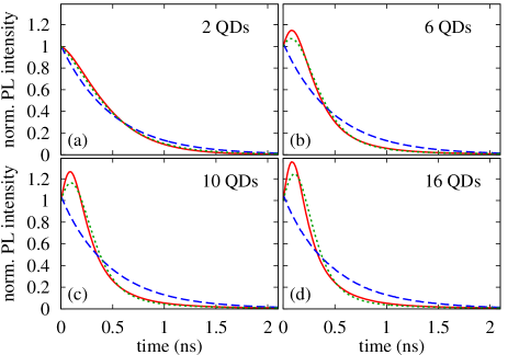
Figure 1: The intensity of luminescence from an ensemble of 2,6,10, and 16 QDs. Red solid lines: $\sigma=0$, $V_{0}=0$; blue dashed lines: $\sigma=0.1$ meV, $V_{0}=0$; green dotted lines: $\sigma=0.1$ meV, $V_{0}=0.5$ meV.

Fig. 1 shows the PL intensity as a function of time for the emission from ensembles of several QDs. If the QDs are identical, $\sigma=0$ and coupled only by the weak dipole interactions, $V_{0}=0$ (red solid lines), the luminescence decay is non-exponential and develops a non-monotonicity (a superradiant peak) as the number of QDs grows. This effect is completely destroyed already by a weak inhomogeneity of the transition energies in the ensemble, $\sigma=0.1$ meV, well below the degree of inhomogeneity expected in a real sample (blue dashed lines). The collective emission effect, with the peaked luminescence, is restored if the QDs are sufficiently strongly coupled, $\sigma=0.1$ meV, $V_{0}=0.5$ meV (green dotted lines) sitek07a . Here, we see the first difference between the case of 2 QDs and a larger number of QDs: the evolution of a strongly coupled 2-QD system nearly exactly follows that for identical dots, while in the other cases, the original photoluminescence decay curve is not completely restored. The reason is that in the 2 QD case the single-exciton eigenstate of a strongly coupled system coincides with the Dicke state, while in a larger ensemble of randomly distributed dots the Dicke states for various exciton numbers are typically not exact eigenstates of the system, although they may have an enhanced overlap with them.

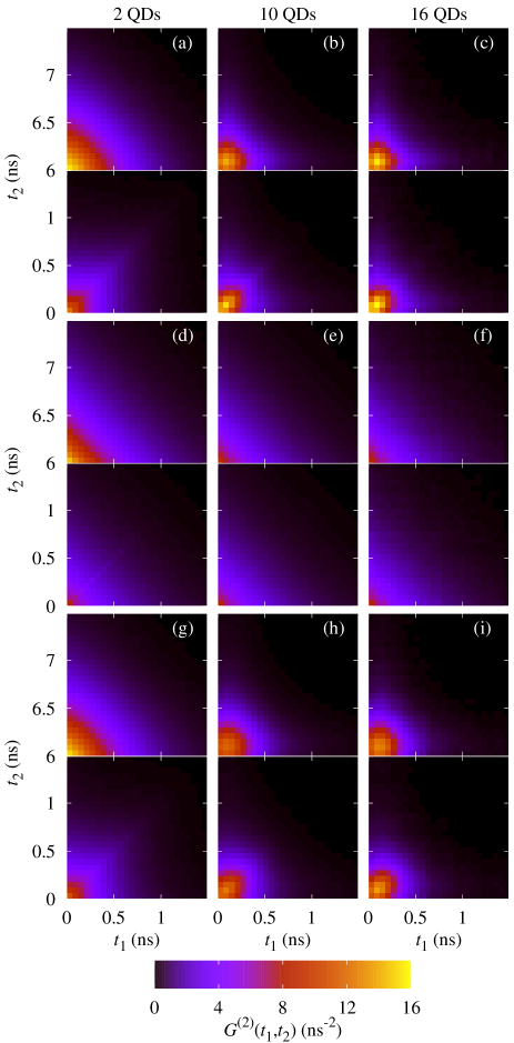
Figure 2: The two-time correlation function $g^{(2)}(t_{1},t_{2})$ for 2,10, and 16 QDs. (a)-(c): $\sigma=0$, $V_{0}=0$; (d)-(f): $\sigma=0.1$ meV, $V_{0}=0$ (g)-(i): $\sigma=0.1$ meV, $V_{0}=0$. The range of $t_{2}$ covers two repetition periods with a certain time interval, where the signal is nearly null, removed.

The interplay between the inhomogeneity and coupling is reflected also in the two-time second order correlation of the photon emission events, as shown in Fig. 2. Each correlation map is shown over one repetition period of the numerical experiment in $t_{1}$ and over two repetition periods in $t_{2}$ (the correlation function for any higher period is the same). The maps show clear differences between the correlations within one repetition period and between different repetition periods, as well as between the cases characterized by different inhomogeneity and inter-dot coupling.

Figs. 2(a)-(c) present the correlation functions for ensembles of identical dots coupled only by the fundamental, weak dipole interactions. The photon emission events in different repetitions of the experiment are uncorrelated. Hence, if $0<t_{1}<T_{\mathrm{rep}}$ and $T_{\mathrm{rep}}<t_{2}<2T_{\mathrm{rep}}$ then $g^{(2)}(t_{1},t_{2})\sim I(t_{1})I(t_{2})$, where $I(t)$ is the luminescence intensity. For identical dots, the emission is non-exponential, with a peak developing at $t>0$ if the number of dots exceeds 2. This is simply reflected in the shape of the correlation function, which has a maximum at $t_{1}=t_{2}>0$ for $N_{\mathrm{QD}}>2$. The picture is very different for the correlations between events within the same repetition period, when the photons are emitted in the course of a single instance of the system evolution. Here, again, the case of 2 QDs (Fig. 2(a)) is exceptional: As explained in Sec. III, after one photon is emitted, there is exactly one left and, according to Eq. (5), the system is projected always on the same single-exciton Dicke state. Therefore, the system evolution after the first emission does not depend on the first emission time. As a result, the correlation function depends only on $\max(t_{1},t_{2})$, hence the characteristic square shaped form of $G^{(2)}(t_{1},t_{2})$ visible in the lower panel of Fig. 2(a). For a larger number of QDs, the system is likely to contain more exciton after emission events that happened at earlier times, hence the further evolution and, in consequence, the correlation function, depends on both time arguments. The square shaped profile of $G^{(2)}$ still remains to some extent visible for 6 QDs (Fig. 2(b)) but is much less pronounced already for 16 QDs (Fig. 2(c)).

If the dispersion of transition energies becomes large enough to prevent the collective emission, as in the cases shown in Figs. 2(d)-(f), then the correlation function shows none of the features discussed above. Now, each photon is emitted by a single and independently evolving QD, hence different emission events are always independent and the correlation function becomes proportional to a product of two exponentially decaying luminescence intensities, $g^{(2)}(t_{1},t_{2})\sim\exp[-\Gamma(t_{1}+t_{2})]$ (see Sec. III). This dependence on $t_{1}+t_{2}$ only is clear in Figs. 2(d)-(f), where the only difference between the correlations within and between the repetitions results from the combinatorial factor ($N(N-1)$ vs. $N^{2}$ photon pairs).

As discussed above, sufficiently strong coupling can restore the characteristic features related to collective luminescence. The shape of the correlation function is also to some extent restored (Figs. 2(g)-(i)) and becomes similar (although not quite identical) to that observed for identical dots.

From now on, we will focus on the correlations within one repetition period.

IV.2 Delay time statistics

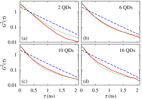
Figure 3: The unnormalized integrated correlation function $G^{(2)}(\tau)$ as a function of the delay $\tau$ for the emission from an ensemble of 2,6,10, and 16 QDs. Red solid lines: $\sigma=0$, $V_{0}=0$; blue dashed lines: $\sigma=0.1$ meV, $V_{0}=0$; green dotted lines: $\sigma=0.1$ meV, $V_{0}=0.5$ meV.

A simple but still very informative characteristics of intensity correlations is the delay-dependent correlation function $G^{(2)}(\tau)$, defined in Sec. II.3, that reflects the statistics of the delay times between pairs of emission events averaged over all the evolution time. This correlation function is shown in Fig. 3 for ensembles of 2,6,10, and 16 QDs. This function is very close to exponential for uncorrelated decay in a strongly inhomogeneous system (blue dashed lines) but becomes non-exponential for a system of more than two identical QDs that emit cooperatively (red lines). This non-exponential dependence on the delay time is restored also by sufficiently strong interactions (green dotted lines).

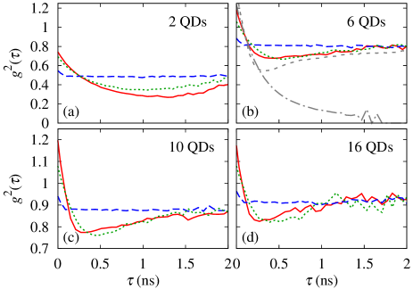
Figure 4: The normalized integrated correlation function $g^{(2)}(\tau)$ as a function of the delay $\tau$ for the emission from an ensemble of 2,6,10, and 16 QDs. Red solid lines: $\sigma=0$, $V_{0}=0$; blue dashed lines: $\sigma=0.1$ meV, $V_{0}=0$; green dotted lines: $\sigma=0.1$ meV, $V_{0}=0.5$ meV. In (c), the grey dashed and dash-dotted lines show the results in the Dicke limit and in the case of vanishing dipole coupling, respectively ($10^{7}$ repetitions in the latter case).

Since the function $G^{(2)}(\tau)$ depends on the actual number of detection events, its magnitude reflects the experimental conditions and only its qualitative features are meaningful. In contrast, its normalized counterpart, $g^{(2)}(\tau)$, defined by Eq. (8), yields intrinsic quantitative information on the photon correlations. This function is shown in Fig. 4. As a result of the normalization by field intensities the form of this function differs considerably from the unnormalized one.

In the case of collective emission (homogeneous ensembles or a sufficiently strong coupling, red solid and green dotted lines in Fig 4, respectively), the value of $g^{(2)}(0)$ is below 1 for a small number of emitters, indicating a non-classical nature of the field (Fig. 4(a)), while it shows a bunching effect, $g^{(2)}(0)>1$, for a larger number of QDs (Fig. 4(b-d)). At finite delays, the normalized correlation function in this case drops down to reach a minimum at a certain time on the order of the spontaneous emission time longer for smaller ensembles) and then increases again up to the a value of $(N-1)/N$ which characterizes uncorrelated emission. The fact that this holds also for a perfectly homogeneous system coupled only by the very weak dipole interactions is quite striking. For a strictly superradiant decay, the correlation function should decay to 0, as discussed for the special case of 2 QDs in Sec. III. Our system differs from that formal limiting case in two respects: First, the distances between the dots are finite (although small), which affects the collective nature of the coupling (technically, $\Gamma_{\alpha\beta}<\Gamma_{0}$ for $\alpha\neq\beta$ in Eq. (1)). Second, the weak but non-zero dipole coupling is always present, as it is of fundamental nature and inseparable from the spontaneous emission process. In order to assess the role of these two factors, in Fig. 4(b) we have included the results for two kinds hypothetical systems: the Dicke limit (negligible distance between the emitters, hence $\Gamma_{\alpha\beta}=\Gamma_{0}$ for all $\alpha,\beta$) with the dipole interactions as for the actual inter-dot distances in our ensemble, as well as an ensemble without any couplings (grey short-dashed and dash-dotted lines, respectively). The comparison of these formal results shows that even in the Dicke limit the behavior of the intensity correlation is similar to the actual one and only upon removing the coupling the non-monotonic behavior of $g^{(2)}(\tau)$ is turned into a monotonic decay. Hence, we conclude that the fundamental dipole coupling, which is too weak to induce any observable traces of collective emission in the luminescence intensity from an inhomogeneous ensemble kozub12 , qualitatively changes the form of the normalized second-order correlation function.

In the case of an inhomogeneous and weakly coupled system, when the decay of both the intensity and the correlations is indistinguishable from exponential (blue dashed lines), the value of the correlation function is almost everywhere constant and equal to $(N-1)/N$, as for uncorrelated emitters. An exception are very short delays, where it shows a weak but clear increase towards $\tau=0$, indicating that some small degree of cooperativity is present in the emission. Hence, also in this case the correlations are more sensitive to the system properties than the intensities.

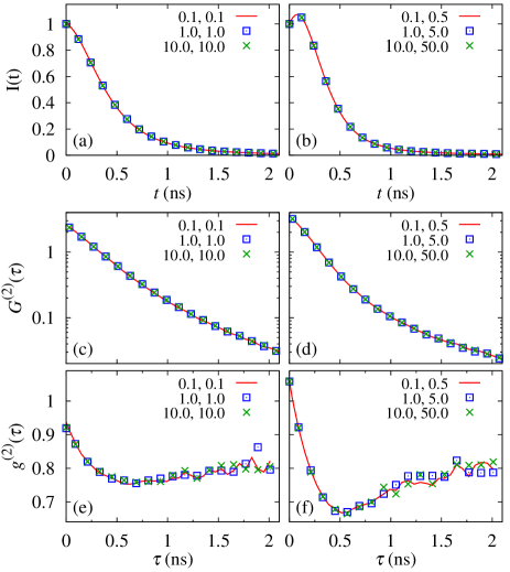
Figure 5: Comparison of luminescence intensities and second-order correlation functions for ensembles with different magnitudes but a fixed ratio between the essential parameters: energy inhomogeneity and coupling strength. The numbers describing the lines and symbols indicate the values of $\sigma$ and $V_{0}$ in meV.

So far, we have discussed ensembles with rather low energy inhomogeneities. However, one can expect that, as soon as both the energy inhomogeneity and typical coupling strengths are much larger than the natural emission line width, the ensemble luminescence should only depend (up to trivial scaling of the time axis) on the ratio of these two parameters. This is strictly the case for 2 QDs, where the energy difference and coupling strength fully characterize the system sitek07a . Although for larger ensembles both these parameters merely characterize a distribution of random values (which is, in addition, non-trivial in the case of the distance-dependent couplings), Fig. 5 shows that such a universal scaling is perfectly valid over two orders of magnitude of these parameters also in the case of larger QD ensembles (here 6 QDs). This holds true not only for the luminescence intensity (Fig. 5(a,b)) but also for the unnormalized and normalized intensity correlation functions $G^{(2)}(\tau)$ and $g^{(2)}(\tau)$ (Fig. 5(c-f)).

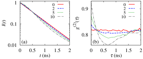
Figure 6: Comparison of the decay of the luminescence intensity $I(t)$ (a) and the normalized correlation function $g^{(2)}(\tau)$ (b) for 6 QDs with $\sigma=10$ meV and various strengths of the coupling $V_{0}$ as shown (in meV). Here, the results have been averaged over $10^{6}$ repetitions.

As the the cooperative nature of the emission proces manifests itself in a qualitative way in the intensity correlations, the correlations statistics may be a better experimental test for such collective effects. Indeed, as we show in Fig. 6, the non-monotonic form of the correlation function $g^{(2)}(\tau)$ [Fig. 6(a)] appears already for inhomogoneous systems in which the the coupling is so weak that the deviation from the exponential luminescence decay [Fig. 6(b)] is almost unnoticeable (in particular, blue dashed lines in Fig. 6, corresponding to $V_{0}=2$ meV$=0.2\sigma$).

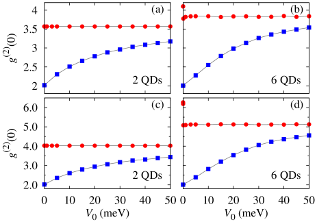
Figure 7: The correlation function $g^{(2)}(0)$ as a function of the coupling parameter $V_{0}$ for a realistic ensemble of two and six QDs (a,c) and assuming the Dicke limit of vanishing geometrical size of the ensemble (b,d). Red circles: identical QDs; Blue squares: non-identical QDs with $\sigma=10$ meV.

A single parameter, quantitatively characterizing the photon-photon correlations, is the value of the correlation function at zero delay, $g^{(2)}(0)$. This is shown in Fig. 7(a,b) for ensembles of 2 and 6 identical QDs (red circles) and for inhomogeneous QD ensembles (blue squares). The effect of the coupling is different in the two cases. An ensemble of identical emitters emits superradiantly in the absence of coupling, while the coupling partly destroys the cooperative emission effect by lifting the degeneracy of the states with a given number of excitons and thus perturbing the Dicke states, which are no more energy eigenstates. As a result, the value of $g^{(2)}(0)$ drops down. An exception is the case of 2 QDs, where the eigenstate of coupled, identical dots coincides with the Dicke state, as discussed above. On the contrary, if the system is energetically inhomogeneous (blue squares), the major effect of the coupling is to overcome the inhomogeneity and to form partly symmetrized eigenstates, which, although not completely identical with the Dicke state for $N_{\mathrm{QD}}>2$, restore the cooperative emission and lead to an increase of $g^{(2)}(0)$.

We note at this point that, apart from the interplay of inhomogeneity and coupling, the cooperative emission form a QD ensemble is affected also by the dependence of the off-diagonal transition rates $\Gamma_{\alpha\beta}$ on the inter-dot distance. Although the spatial sizes of the ensembles modeled here are always smaller than the wave length (about 1 $\mu$m in the medium, compared to 30 nm average distance between the neighboring QDs), the finite-size effect is quantitatively noticeable. This is illustrated by Fig. 7(c,d), where the results as in the two upper panels are shown but this time assuming the (formal) Dicke limit of a very small ensemble, with $\Gamma_{\alpha\beta}=\Gamma_{0}$. While the qualitative dependence of $g^{(2)}(0)$ is the same as in the realistic case, the values are clearly higher.

V Conclusions

We have studied the second order correlation function (intensity autocorrelation) on sub-nanosecond time scales for the spontaneous emission from inhomogeneous planar ensembles of coupled QDs using the quantum jump approach to numerical simulations of the open system dynamics, which mimics a recently developed experimental technique.

We have shown that the cooperative nature of the emission manifests itself not only by non-exponential decay of luminescence, but also in the particular form of both the normalized and unnormalized correlation functions. The collective emission case corresponds either to the rather hypothetical limit of a very homogeneous QD ensemble or to a realistic case of en inhomogeneous ensemble of coupled dots. The signatures of collective emission in the intensity correlations are the same in both these cases.

The normalized correlation function is of particular interest as it shows qualitative features (non-monotonic delay dependence) for weakly coupled inhomogeneous systems for which the non-exponential character of luminescence decay is so weak that it may be hard to notice experimentally. Thus, we conclude that the photon-photon delay time statistics may be a better experimental probe of cooperative effects than the time-resolved luminescence intensity.

- (1) M. Scheibner, T. Schmidt, L. Worschech, A. Forchel, G. Bacher, T. Passow, and D. Hommel, Nat. Phys. 3, 106 (2007).
- (2) Y. I. Mazur, V. G. Dorogan, J. E. Marega, G. G. Tarasov, D. F. Cesar, V. Lopez-Richard, G. E. Marques, and G. J. Salamo, Appl. Phys. Lett. 94, 123112 (2009).
- (3) Y. Mazur, V. G. Dorogan, E. Marega, D. F. Cesar, V. Lopez-Richard, G. E. Marques, Z. Zhuchenko, G. G. Tarasov, and G. J. Salamo, Nano. Res. Lett. 5, 991 (2010).
- (4) N. Skribanowitz, I. P. Herman, J. C. MacGilvray, and M. S. Feld, Phys. Rev. Lett. 30, 309 (1973).
- (5) M. Bayer and A. Forchel, Phys. Rev. B 65, 041308 (2002).
- (6) A. Sitek and P. Machnikowski, Phys. Rev. B 75, 035328 (2007).
- (7) M. Kozub, b. Pawicki, P. Machnikowski, and Å. Pawicki, Phys. Rev. B 86, 121305 (2012).
- (8) S. M. Ulrich, C. Gies, S. Ates, J. Wiersig, S. Reitzenstein, C. Hofmann, A. Löffler, A. Forchel, F. Jahnke, and P. Michler, Phys. Rev. Lett. 98, 043906 (2007).
- (9) G. Callsen, A. Carmele, G. Hönig, C. Kindel, J. Brunnmeier, M. R. Wagner, E. Stock, J. S. Reparaz, A. Schliwa, S. Reitzenstein, A. Knorr, A. Hoffmann, S. Kako, and Y. Arakawa, Phys. Rev. B 87, 245314 (2013).
- (10) M. Davanço, C. S. Hellberg, S. Ates, A. Badolato, and K. Srinivasan, Phys. Rev. B 89, 161303 (2014).
- (11) J. Wiersig, C. Gies, F. Jahnke, M. Assmann, T. Berstermann, M. Bayer, C. Kistner, S. Reitzenstein, C. Schneider, S. Höfling, A. Forchel, C. Kruse, J. Kalden, and D. Hommel, Nature 460, 245 (2009).
- (12) M. Aß mann, F. Veit, M. Bayer, C. Gies, F. Jahnke, S. Reitzenstein, S. Höfling, L. Worschech, and A. Forchel, Phys. Rev. B 81, 165314 (2010).
- (13) M. Assmann, F. Veit, J.-S. Tempel, T. Berstermann, H. Stolz, M. van der Poel, J. r. M. Hvam, and M. Bayer, Opt. Express 18, 20229 (2010).
- (14) V. V. Temnov and U. Woggon, Opt. Express 17, 5774 (2009).
- (15) A. Auffèves, D. Gerace, S. Portolan, A. Drezet, M. França Santos, and M. F. Santos, New J. Phys. 13, 093020 (2011).
- (16) S. Ritter, P. Gartner, C. Gies, and F. Jahnke, Opt. Express 18, 9909 (2010).
- (17) Z. Harsij, M. Bagheri Harouni, R. Roknizadeh, and M. H. Naderi, Phys. Rev. A 86, 063803 (2012).
- (18) Y. Su, M. Richter, A. Knorr, D. Bimberg, and A. Carmele, Phys. status solidi - Rapid Res. Lett. 4, 289 (2010).
- (19) M. J. Stephen, J. Chem. Phys. 40, 669 (1964).
- (20) R. H. Lehmberg, Phys. Rev. A 2, 883 (1970).
- (21) A. Varfolomeev, Zh. Eksp. Teor. Fiz. 59, 1702 (1970).
- (22) A. Baumgartner, E. Stock, A. Patanè, L. Eaves, M. Henini, and D. Bimberg, Phys. Rev. Lett. 105, 257401 (2010).
- (23) H.-P. Breuer and F. Petruccione, The Theory of Open Quantum Systems (Oxford University Press, Oxford, 2007).
- (24) C. W. Gardiner and P. Zoller, Quantum noise: a handbook of Markovian and non-Markovian quantum stochastic methods with applications to quantum optics (Springer, Berlin, 2004).