Div First-Order System LL* (FOSLL*) for Second-Order Elliptic Partial Differential Equations

Abstract

The first-order system LL* (FOSLL*) approach for general second-order elliptic partial differential equations was proposed and analyzed in [10], in order to retain the full efficiency of the $L^{2}$ norm first-order system least-squares (FOSLS) approach while exhibiting the generality of the inverse-norm FOSLS approach. The FOSLL* approach in [10] was applied to the div-curl system with added slack variables, and hence it is quite complicated. In this paper, we apply the FOSLL* approach to the div system and establish its well-posedness. For the corresponding finite element approximation, we obtain a quasi-optimal a priori error bound under the same regularity assumption as the standard Galerkin method, but without the restriction to sufficiently small mesh size. Unlike the FOSLS approach, the FOSLL* approach does not have a free a posteriori error estimator, we then propose an explicit residual error estimator and establish its reliability and efficiency bounds.

Key words. LL* method, least-squares method, a priori error estimate, a posteriori error estimate, elliptic equations.

AMS(MOS) subject classifications. 65M60, 65M15

1 Introduction

There are substantial interests in the use of least squares principles for the approximate solution of partial differential equations with applications in both solid and fluid mechanics. Many least-squares methods for the scalar elliptic partial differential equations have been proposed and analyzed, [3, 15]. Their numerical properties depend on choices such as the first-order system and the least-squares norm. Loosely speaking, there are three types of least-squares methods: the inverse approach, the div approach, and the div-curl approach. The inverse approach employs an inverse norm that is further replaced by either the weighted mesh-dependent norm (see [2]) or the discrete $H^{-1}$ norm (see [7]) for computational feasibility. Both the div and the div-curl approaches use the $L^{2}$ norm and the corresponding homogeneous least-squares functionals are equivalent to the $H({\rm div})\times H^{1}$ and the $\left(H({\rm div})\cap H({\rm curl})\right)\times H^{1}$ norms, respectively. The div approach based on the flux-pressure formulation has been studied by many researchers (see, e.g., [4, 8, 14, 16]). The div-curl approach [9] has also been well studied.

In order to retain the full efficiency of the $L^{2}$ norm first-order system least-squares (FOSLS) approach while exhibiting the generality of the inverse-norm FOSLS approach, the first-order system LL* (FOSLL*) approach for general second-order elliptic partial differential equations was proposed and analyzed in [10]. The FOSLL* approach was applied to the div-curl system, whose adjoint system is an underdetermined system and hence is not suitable for FOSLL*. This difficulty was overcome by carefully adding slack variables to the div-curl system. But the resulting approach is quite complicated.

Our purpose here is to study the FOSLL* approach applying to the div system. Without adding any slack variables to the div system, the resulting approach is much simpler than that in [10]. By showing that the bilinear form of the FOSLL* approach is coercive and bounded and that the linear form is bounded with respect to a weighted $H({\rm div})\times H^{1}$ norm, we establish the well-posedness of the FOSLL* approach. Under the same regularity assumption as the standard Galerkin method, but without the restriction to sufficiently small mesh size, we obtain a quasi-optimal a priori error bound for the corresponding finite element approximation. Note that this assumption is weaker than that for the div FOSLS [11]. Unlike the FOSLS approach, the FOSLL* approach does not have a free a posteriori error estimator, thus we study an explicit residual error estimator and establish its reliability and efficiency bounds.

The paper is organized as follows. In Section 2 we introduce mathematical equations for the second-order scalar elliptic partial differential equations and its div first-order system, and we then derive the FOSLL* variational formulation and establish its well-posedness. In Section 3, the FOSLL* finite element approximation is described. A priori and a posteriori error estimations are obtained in Sections 4 and 5 respectively. In Section 6, we present numerical results.

1.1 Notation

We use the standard notations and definitions for the Sobolev spaces $H^{s}(\Omega)^{d}$ and $H^{s}(\partial\Omega)^{d}$ for $s\geq 0$. The standard associated inner products are denoted by $(\cdot,\,\cdot)_{s,\Omega}$ and $(\cdot,\,\cdot)_{s,\partial\Omega}$, and their respective norms are denoted by $\|\cdot\|_{s,\Omega}$ and $\|\cdot\|_{s,\partial\Omega}$. (We suppress the superscript $d$ because the dependence on dimension will be clear by context. We also omit the subscript $\Omega$ from the inner product and norm designation when there is no risk of confusion.) For $s=0$, $H^{s}(\Omega)^{d}$ coincides with $L^{2}(\Omega)^{d}$. In this case, the inner product and norm will be denoted by $\|\cdot\|$ and $(\cdot,\,\cdot)$, respectively. Set

$$H^{1}_{D}(\Omega):=\{q\in H^{1}(\Omega)\,:\,q=0\,\,\mbox{on}\,\,\Gamma_{D}\}.$$

When $\Gamma=\partial\Omega$, denote $H^{1}_{D}(\Omega)$ by $H^{1}_{0}(\Omega)$. Finally, set

$$H({\rm div};\Omega)=\{{\bf v}\in L^{2}(\Omega)^{d}\,:\,\nabla\cdot{\bf v}\in L^{2}(\Omega)\},$$

which is a Hilbert space under the norm

$$\|{\bf v}\|_{H({\rm div};\,\Omega)}=\left(\|{\bf v}\|^{2}+\|\nabla\cdot{\bf v}\|^{2}\right)^{1/2},$$

and define the subspace

$$H_{N}({\rm div};\Omega)=\{{\bf v}\in H({\rm div};\Omega)\,:\,{\bf n}\cdot{\bf v}=0\,\,\mbox{on}\,\,\Gamma_{N}\}.$$

2 First-Order System LL* Formulation

Let $\Omega$ be a bounded, open, connected subset of $\Re^{d}$ ($d=2$ or $3$) with a Lipschitz continuous boundary $\partial\Omega$. Denote by ${\bf n}=(n_{1},\,...\,,\,n_{d})$ the outward unit vector normal to the boundary. We partition the boundary of the domain $\Omega$ into two open subsets $\Gamma_{D}$ and $\Gamma_{N}$ such that $\partial\Omega=\bar{\Gamma}_{D}\cup\bar{\Gamma}_{N}$ and $\Gamma_{D}\cap\Gamma_{N}=\emptyset$. For simplicity, we assume that $\Gamma_{D}$ is not empty (i.e., $\mbox{mes}\,(\Gamma_{D})\not=0$) and is connected.

2.1 Second-Order Elliptic Problem

Consider the following second-order elliptic boundary value problem:

$$-\nabla\cdot\,(A\nabla\,u)+{\bf b}\cdot\nabla\,u+a\,u=f\quad\mbox{in}\,\,\Omega$$ (2.1)

with boundary conditions

$$u=g_{{}_{D}}\quad\mbox{on}\,\,\Gamma_{D}\quad\mbox{and}\quad-A\nabla\,u\cdot{\bf n}=g_{{}_{N}}\quad\mbox{on}\,\,\Gamma_{N},$$ (2.2)

where the symbols $\nabla\cdot$ and $\nabla$ stand for the divergence and gradient operators, respectively; $A$ is a given $d\times d$ tensor-valued function; ${\bf b}\in L^{\infty}(\Omega)^{d}$ and $a\in L^{\infty}(\Omega)$ are given vector- and scalar-valued functions, respectively; and $f$ is a given scalar function. Assume that $A$ is uniformly symmetric positive definite: there exist positive constants $0<\Lambda_{0}\leq\Lambda_{1}$ such that

$$\Lambda_{0}\boldsymbol{\xi}^{T}\boldsymbol{\xi}\leq\boldsymbol{\xi}^{T}A\boldsymbol{\xi}\leq\Lambda_{1}\boldsymbol{\xi}^{T}\boldsymbol{\xi}$$

for all $\boldsymbol{\xi}\in\Re^{d}$ and almost all $x\in\overline{\Omega}$. The corresponding variational form of system (2.1)-(2.2) is to find $u\in H^{1}(\Omega)$ such that $u|_{\Gamma_{D}}=g_{{}_{D}}$ and that

$$a(u,\,v)=(f,\,v)-\int_{\Gamma_{N}}g_{{}_{D}}v\,ds\quad\forall\,\,v\in H^{1}_{D}(\Omega),$$ (2.3)

where the bilinear form is defined by

$$a(u,\,v)=(A\nabla\,u,\,\nabla\,v)+({\bf b}\cdot\nabla\,u+a\,u,\,v).$$

The dual problem of (2.3) is to find $z\in H^{1}(\Omega)$ such that $z|_{\Gamma_{D}}=g_{{}_{D}}$ and that

$$\hat{a}(\phi,\,z)=(f,\,v)-\int_{\Gamma_{N}}g_{{}_{N}}v\,ds\quad\forall\,\,\phi\in H^{1}_{D}(\Omega),$$ (2.4)

where the bilinear form is defined by

$$\hat{a}(\phi,\,z)=\left(\nabla\,\phi,\,(A\,\nabla+{\bf b})\,z\right)+(\phi,\,a\,z).$$

Assume that both problems (2.3) and (2.4) have unique solutions and, for simplicity of the presentation, satisfy the full $H^{2}$ regularity estimates:

$$\|u\|_{2}\leq C\,\|f\|\quad\mbox{and}\quad\|z\|_{2}\leq C\,\|f\|.$$ (2.5)

Here and thereafter, we use $C$ with or without subscripts in this paper to denote a generic positive constant, possibly different at different occurrences, that is independent of the mesh size $h$ but may depend on the domain $\Omega$.

2.2 First-Order System

Introducing the flux (vector) variable

$$\mbox{\boldmath$\sigma$}=-A\,\nabla u,$$

the scalar elliptic problem in (2.1)-(2.2) may be rewritten as the following first-order partial differential system:

$$\left\{\begin{array}[]{lcclc}A^{-1}\mbox{\boldmath$\sigma$}+\nabla u&=&{\bf 0}&\quad\mbox{in}&\Omega,\\[5.69054pt] \nabla\cdot\mbox{\boldmath$\sigma$}-{\bf b}\cdot A^{-1}\mbox{\boldmath$\sigma$}+a\,u&=&f&\quad\mbox{in}&\Omega\end{array}\right.$$ (2.6)

with boundary conditions

$$u=g_{{}_{D}}\quad\mbox{on}\,\,\Gamma_{D}\quad\mbox{and}\quad{\bf n}\cdot\mbox{\boldmath$\sigma$}=g_{{}_{N}}\quad\mbox{on}\,\,\Gamma_{N}.$$ (2.7)

Let

$${\cal L}=\left(\begin{array}[]{cc}A^{-1}&\nabla\\[5.69054pt] \nabla\cdot-{\bf b}\cdot A^{-1}&a\end{array}\right),\quad{\cal U}=\left(\begin{array}[]{c}\mbox{\boldmath$\sigma$}\\[5.69054pt] u\end{array}\right),\quad\mbox{and}\quad{\cal F}=\left(\begin{array}[]{c}{\bf 0}\\[5.69054pt] f\end{array}\right),$$

then (2.6) may be rewritten as

$${\cal L}\,{\cal U}={\cal F}.$$ (2.8)

2.3 Div FOSLL* Variational Formulation

Multiplying test function ${\cal V}=(\mbox{\boldmath$\tau$},\,v)^{t}\in H_{N}({\rm div};\Omega)\times H^{1}_{D}(\Omega)$, integrating over the domain $\Omega$, and using integration by parts, we have

$$(f,\,v) = \langle{\cal F},\,{\cal V}\rangle=\langle{\cal L}\,{\cal U},\,{\cal V}\rangle$$

$$= (A^{-1}\mbox{\boldmath$\sigma$}+\nabla u,\,\mbox{\boldmath$\tau$})+(\nabla\cdot\mbox{\boldmath$\sigma$}-{\bf b}\cdot A^{-1}\mbox{\boldmath$\sigma$}+a\,u,\,v)$$

$$= (\mbox{\boldmath$\sigma$},\,A^{-1}\mbox{\boldmath$\tau$})-(\mbox{\boldmath$\sigma$},\,\nabla\,v)+\int_{\partial\Omega}(\mbox{\boldmath$\sigma$}\cdot{\bf n})\,v\,ds-(\mbox{\boldmath$\sigma$},\,A^{-1}{\bf b}\,v)$$

$$-(u,\,\nabla\cdot\,\mbox{\boldmath$\tau$})+\int_{\partial\Omega}(\mbox{\boldmath$\tau$}\cdot{\bf n})\,u\,ds+(u,\,a\,v)$$

$$= \big{(}\mbox{\boldmath$\sigma$},\,A^{-1}\mbox{\boldmath$\tau$}-(\nabla+A^{-1}{\bf b})\,v\big{)}+\big{(}u,\,a\,v-\nabla\cdot\mbox{\boldmath$\tau$}\big{)}+\int_{\Gamma_{N}}g_{{}_{N}}v\,ds+\int_{\Gamma_{D}}g_{{}_{D}}(\mbox{\boldmath$\tau$}\cdot{\bf n})\,ds$$

$$= \langle{\cal U},\,{\cal L}^{*}\,{\cal V}\rangle+g(\mbox{\boldmath$\tau$},\,v),$$

where the formal adjoint of ${\cal L}$ and the boundary functional are defined by

$${\cal L}^{*}=\left(\begin{array}[]{cc}A^{-1}&-(\nabla+A^{-1}{\bf b})\\[5.69054pt] -\nabla\cdot&a\end{array}\right)\quad\mbox{and}\quad g(\mbox{\boldmath$\tau$},\,v)=\int_{\Gamma_{N}}g_{{}_{N}}v\,ds+\int_{\Gamma_{D}}g_{{}_{D}}(\mbox{\boldmath$\tau$}\cdot{\bf n})\,ds,$$

respectively.

Without loss of generality, we assume that $a\not=0$ in this paper and let

$${\cal A}=\left(\begin{array}[]{cc}A&0\\[5.69054pt] 0&a^{-1}\end{array}\right).$$

Let ${\cal W}=(\mbox{\boldmath$\eta$},\,w)^{t}$ satisfy

$${\cal U}={\cal A}\,{\cal L}^{*}\,{\cal W}=\left(\begin{array}[]{c}\mbox{\boldmath$\eta$}-(A\nabla+{\bf b})\,w\\[5.69054pt] -a^{-1}\nabla\cdot\mbox{\boldmath$\eta$}+w\end{array}\right),$$ (2.9)

then we have

$$\langle{\cal A}\,{\cal L}^{*}\,{\cal W},\,{\cal L}^{*}\,{\cal V}\rangle=(f,\,v)-g(\mbox{\boldmath$\tau$},\,v)\equiv f(\mbox{\boldmath$\tau$},\,v).$$

Now, our div FOSLL* variational formulation is to find $(\mbox{\boldmath$\eta$},\,w)\in H_{N}({\rm div};\Omega)\times H^{1}_{D}(\Omega)$ such that

$$b(\mbox{\boldmath$\eta$},\,w;\,\mbox{\boldmath$\tau$},\,v)=f(\mbox{\boldmath$\tau$},\,v),\quad\forall\,\,(\mbox{\boldmath$\tau$},\,v)\in H_{N}({\rm div};\Omega)\times H^{1}_{D}(\Omega),$$ (2.10)

where the bilinear form $b(\cdot,\,\cdot)$ is defined by

$$b(\mbox{\boldmath$\eta$},\,w;\,\mbox{\boldmath$\tau$},\,v)=\langle{\cal A}\,{\cal L}^{*}\,{\cal W},\,{\cal L}^{*}\,{\cal V}\rangle$$

$$= \left(\mbox{\boldmath$\eta$}-(A\,\nabla+{\bf b})\,w,\,A^{-1}\mbox{\boldmath$\tau$}-(\nabla+A^{-1}{\bf b})\,v\right)+(a^{-1}\nabla\cdot\,\mbox{\boldmath$\eta$}-w,\,\nabla\cdot\,\mbox{\boldmath$\tau$}-a\,v).$$

Note that both non-homogenous Dirichlet and Neumann boundary conditions are imposed weekly.

Remark 2.1.

For any $(\mbox{\boldmath$\eta$},\,w),\,\,(\mbox{\boldmath$\tau$},\,v)\in H_{N}({\rm div};\Omega)\times H^{1}_{D}(\Omega)$, integration by parts gives

$$(\nabla w,\mbox{\boldmath$\tau$})+(w,\nabla\cdot\mbox{\boldmath$\tau$})=(\nabla v,\mbox{\boldmath$\eta$})+(v,\nabla\cdot\mbox{\boldmath$\eta$})=0.$$

Hence, the bilinear form $b(\cdot,\,\cdot)$ has of the form

$$b(\mbox{\boldmath$\eta$},\,w;\,\mbox{\boldmath$\tau$},\,v) \!\!=\!\! (A^{-1}\mbox{\boldmath$\eta$},\,\mbox{\boldmath$\tau$})+(a^{-1}\nabla\cdot\mbox{\boldmath$\eta$},\,\nabla\cdot\mbox{\boldmath$\tau$})+(A\nabla w,\,\nabla v)+(a\,w,\,v)$$

$$\!\!\!-({\bf b}\,w,\,A^{-1}\mbox{\boldmath$\tau$})-(A^{-1}\mbox{\boldmath$\eta$},\,{\bf b}\,v)+({\bf b}\,w,\,\nabla v)+(\nabla w,\,{\bf b}\,v)+(A^{-1}{\bf b}\,w,\,{\bf b}\,v).$$

In the case that ${\bf b}={\bf 0}$ and $a\not=0$, i.e., the diffusion-reaction problem, the div FOSLL* problem in (2.10) is decoupled. More specifically, $w\in H^{1}_{D}(\Omega)$ is the solution of

$$(A\nabla w,\,\nabla v)+(a\,w,\,v)=(f,\,v)-\int_{\Gamma_{N}}g_{{}_{N}}v\,ds,\quad\forall\,\,v\in H^{1}_{D}(\Omega),$$

and $\mbox{\boldmath$\eta$}\in H_{N}({\rm div};\Omega)$ satisfies

$$(A^{-1}\mbox{\boldmath$\eta$},\,\mbox{\boldmath$\tau$})+(a^{-1}\nabla\cdot\mbox{\boldmath$\eta$},\,\nabla\cdot\mbox{\boldmath$\tau$})=-\int_{\Gamma_{D}}g_{{}_{D}}(\mbox{\boldmath$\tau$}\cdot{\bf n})\,ds.$$

Note that the problem for $w$ is similar to the standard variational formulation for the diffusion-reaction problem, but the non-homogeneous Dirichlet boundary condition is weakly imposed here.

Remark 2.2.

In the case that $a=0$, let ${\cal A}=\mbox{diag}\,(A,\,1)$, then ${\cal W}=(\mbox{\boldmath$\eta$},\,w)^{t}$ satisfy

$${\cal U}={\cal A}\,{\cal L}^{*}{\cal W}=\left(\begin{array}[]{c}\mbox{\boldmath$\eta$}-(A\nabla+{\bf b})\,w\\[5.69054pt] -\nabla\cdot\mbox{\boldmath$\eta$}\end{array}\right).$$ (2.11)

The corresponding bilinear form is modified as follows

$$b(\mbox{\boldmath$\eta$},\,w;\,\mbox{\boldmath$\tau$},\,v)=\big{(}\mbox{\boldmath$\eta$}-(A\,\nabla+{\bf b})\,w,\,A^{-1}\mbox{\boldmath$\tau$}-(\nabla+A^{-1}{\bf b})\,v\big{)}+\big{(}\nabla\cdot\,\mbox{\boldmath$\eta$},\,\nabla\cdot\,\mbox{\boldmath$\tau$}\big{)}.$$

2.4 Well-Posedness

Denote by

$$|\!|\!|v|\!|\!|_{1}=\left(\|a^{1/2}v\|^{2}+\|A^{1/2}\nabla\,v\|^{2}\right)^{1/2}\mbox{ and }\,\,|\!|\!|\mbox{\boldmath$\tau$}|\!|\!|_{H({\rm div})}=\left(\|A^{-1/2}\mbox{\boldmath$\tau$}\|^{2}+\|a^{-1/2}\nabla\cdot\mbox{\boldmath$\tau$}\|^{2}\right)^{1/2}$$

the weighted $H^{1}(\Omega)$ and $H({\rm div};\Omega)$ norms, respectively. Let

$$|\!|\!|(\mbox{\boldmath$\tau$},\,v)|\!|\!|=\left(|\!|\!|v|\!|\!|^{2}_{1}+|\!|\!|\mbox{\boldmath$\tau$}|\!|\!|^{2}_{H({\rm div})}\right)^{1/2}.$$

The following theorem establishes the coercivity and continuity of the bilinear form.

Theorem 2.3.

The bilinear form $b(\cdot,\,\cdot)$ is coercive and continuous in $H_{N}({\rm div};\Omega)\times H^{1}_{D}(\Omega)$, i.e., there exist positive constant $\alpha$ and $C$, depending on bounds of the coefficients ($A$, ${\bf b}$, and $a$), such that

$$\alpha\,|\!|\!|(\mbox{\boldmath$\tau$},\,{\bf v})|\!|\!|^{2}\leq b(\mbox{\boldmath$\tau$},\,v;\,\mbox{\boldmath$\tau$},\,v)$$ (2.12)

and that

$$b(\mbox{\boldmath$\eta$},\,w;\,\mbox{\boldmath$\tau$},\,v)\leq C\,|\!|\!|(\mbox{\boldmath$\eta$},\,w)|\!|\!|\,|\!|\!|(\mbox{\boldmath$\tau$},\,v)|\!|\!|$$ (2.13)

for all $(\mbox{\boldmath$\eta$},\,u),\,\,(\mbox{\boldmath$\tau$},\,v)\in H_{N}({\rm div};\Omega)\times H^{1}_{D}(\Omega)$.

A similar result to that of Theorem 2.3 was proved in [8]. For the convenience of readers, we provide a comprehensive proof here.

Proof.

(2.13) is a direct consequence of the Cauchy-Schwarz and the triangle inequalities and the bounds of the coefficients ($A$, ${\bf b}$, and $a$) of the underlying problem. To show the validity of (2.12), we first establish that

$$|\!|\!|(\mbox{\boldmath$\tau$},\,v)|\!|\!|^{2}\leq C\,\left(b(\mbox{\boldmath$\tau$},\,v;\,\mbox{\boldmath$\tau$},\,v)+\|v\|^{2}\right)$$ (2.14)

for all $(\mbox{\boldmath$\tau$},\,v)\in H_{N}({\rm div};\Omega)\times H^{1}_{D}(\Omega)$. To this end, integrating by parts gives

$$(\mbox{\boldmath$\tau$},\,\nabla\,v)=(-a^{-1/2}\nabla\cdot\mbox{\boldmath$\tau$}+a^{1/2}v,\,a^{1/2}v)-(a\,v,\,v).$$

It then follows from the Cauchy-Schwarz inequality that

$$\|A^{1/2}\nabla\,v\|^{2}+\|a^{1/2}v\|^{2}$$

$$= \left(A^{1/2}\nabla\,v-A^{-1/2}(\mbox{\boldmath$\tau$}-{\bf b}\,v),\,A^{1/2}\nabla\,v\right)+\left(a^{1/2}v-a^{-1/2}\nabla\cdot\mbox{\boldmath$\tau$},\,a^{1/2}v\right)-\left({\bf b}\,v,\,\nabla\,v\right)$$

$$\leq \left(\|A^{1/2}\nabla\,v-A^{-1/2}(\mbox{\boldmath$\tau$}-{\bf b}\,v)\|+C\,\|v\|\right)\|A^{1/2}\nabla\,v\|+\|a^{-1/2}\nabla\cdot\mbox{\boldmath$\tau$}-a^{1/2}v\|\,\|a^{1/2}v\|,$$

which implies

$$\|A^{1/2}\nabla\,v\|^{2}+\|a^{1/2}v\|^{2}\leq C\,\left(b(\mbox{\boldmath$\tau$},\,v;\,\mbox{\boldmath$\tau$},\,v)+\|v\|^{2}\right).$$ (2.15)

By the triangle inequality and (2.15), we have that

$$\|A^{-1/2}\mbox{\boldmath$\tau$}\| \leq \left(\|A^{-1/2}(\mbox{\boldmath$\tau$}-{\bf b}\,v)-A^{1/2}\nabla\,v\|+\|A^{1/2}\nabla\,v\|+C\,\|v\|\right)$$

$$\leq C\,\left(b(\mbox{\boldmath$\tau$},\,v;\,\mbox{\boldmath$\tau$},\,v)^{1/2}+\|v\|\right).$$

and that

$$\|a^{-1/2}\nabla\cdot\mbox{\boldmath$\tau$}\|\leq\|a^{-1/2}\nabla\cdot\mbox{\boldmath$\tau$}-a^{1/2}v\|+\|a^{1/2}v\|\leq C\,\left(b(\mbox{\boldmath$\tau$},\,v;\,\mbox{\boldmath$\tau$},\,v)+\|v\|^{2}\right).$$

Combining the above three inequalities yields (2.14).

With (2.14), we now show the validity of (2.12) by the standard compactness argument. To this end, assume that (2.12) is not true. This implies that there exists a sequence $\{\mbox{\boldmath$\tau$}_{n},\,v_{n}\}\in H_{N}({\rm div};\,\Omega)\times H_{D}^{1}(\Omega)$ such that

$$|\!|\!|\mbox{\boldmath$\tau$}_{n}|\!|\!|^{2}_{H({\rm div})}+|\!|\!|v_{n}|\!|\!|^{2}_{1}=1\quad\mbox{and}\quad b(\mbox{\boldmath$\tau$}_{n},\,v_{n};\,\mbox{\boldmath$\tau$}_{n},\,v_{n})\leq\displaystyle\frac{1}{n}.$$ (2.16)

Since $H^{1}_{D}(\Omega)$ is compactly contained in $L^{2}(\Omega)$, there exists a subsequence $\{v_{n_{k}}\}\in H^{1}_{D}(\Omega)$ which converges in $L^{2}(\Omega)$. For any $k,\,\,l$ and $(\mbox{\boldmath$\tau$}_{n_{k}},\,v_{n_{k}})$, $(\mbox{\boldmath$\tau$}_{n_{l}},\,v_{n_{l}})\in H_{N}({\rm div};\,\Omega)\times H^{1}_{D}(\Omega)$, it follows from (2.14) and the triangle inequality that

$$|\!|\!|\mbox{\boldmath$\tau$}_{n_{k}}-\mbox{\boldmath$\tau$}_{n_{l}}|\!|\!|^{2}_{H({\rm div})}+|\!|\!|v_{n_{k}}-v_{n_{l}}|\!|\!|^{2}_{1,\,\Omega}$$

$$\leq C\left(b(\mbox{\boldmath$\tau$}_{n_{k}}-\mbox{\boldmath$\tau$}_{n_{l}},\,v_{n_{k}}-v_{n_{l}};\,\mbox{\boldmath$\tau$}_{n_{k}}-\mbox{\boldmath$\tau$}_{n_{l}},\,v_{n_{k}}-v_{n_{l}})+\|v_{n_{k}}-v_{n_{l}}\|^{2}\right)$$

$$\leq C\left(b(\mbox{\boldmath$\tau$}_{n_{k}},\,v_{n_{k}};\,\mbox{\boldmath$\tau$}_{n_{k}},\,v_{n_{k}})+b(\mbox{\boldmath$\tau$}_{n_{l}},\,v_{n_{l}};\,\mbox{\boldmath$\tau$}_{n_{l}},\,v_{n_{l}})+\|v_{n_{k}}-v_{n_{l}}\|^{2}\right)$$

$$\to 0,$$

as $k,\,\,l\to\infty$. This implies that $(\mbox{\boldmath$\tau$}_{n_{k}},\,v_{n_{k}})$ is a Cauchy sequence in the complete space $H_{N}({\rm div};\,\Omega)\times H^{1}_{D}(\Omega)$. Hence, there exists $(\mbox{\boldmath$\tau$},\,v)\in H_{N}({\rm div};\,\Omega)\times H^{1}_{D}(\Omega)$ such that

$$\lim\limits_{k\to\infty}\left(|\!|\!|\mbox{\boldmath$\tau$}_{n_{k}}-\mbox{\boldmath$\tau$}|\!|\!|_{H({\rm div})}+|\!|\!|v_{n_{k}}-v|\!|\!|_{1}\right)=0.$$

Next, we show that

$$v=0\quad\mbox{and}\quad\mbox{\boldmath$\tau$}={\bf 0},$$ (2.17)

which contradict with (2.16) that

$$0=|\!|\!|\mbox{\boldmath$\tau$}|\!|\!|^{2}_{H({\rm div})}+|\!|\!|v|\!|\!|^{2}_{1}=\lim\limits_{k\to\infty}\left(|\!|\!|\mbox{\boldmath$\tau$}_{n_{k}}|\!|\!|^{2}_{H({\rm div})}+|\!|\!|v_{n_{k}}|\!|\!|^{2}_{1}\right)=1.$$

To this end, for any $\phi\in H^{1}_{D}(\Omega)$, integration by parts, the Cauchy-Schwarz inequality, and (2.16) give

$$\hat{a}(\phi,\,v_{n_{k}}) = \left(\nabla\,\phi,\,(A\,\nabla+{\bf b})\,v_{n_{k}}\right)+(\phi,\,a\,v_{n_{k}})$$

$$= \left(\nabla\phi,\,(A\,\nabla+{\bf b})\,v_{n_{k}}-\mbox{\boldmath$\tau$}_{n_{k}}\right)+(\phi,\,a\,v_{n_{k}}-\nabla\cdot\mbox{\boldmath$\tau$}_{n_{k}})$$

$$\leq b(\mbox{\boldmath$\tau$}_{n_{k}},\,v_{n_{k}};\,\mbox{\boldmath$\tau$}_{n_{k}},\,v_{n_{k}})^{1/2}|\!|\!|\phi|\!|\!|_{1}\leq\left(\displaystyle\frac{1}{n_{k}}\right)^{1/2}|\!|\!|\phi|\!|\!|_{1}.$$

Since $\lim_{k\to\infty}v_{n_{k}}=v$ in $H^{1}(\Omega)$, we then have

$$|\hat{a}(\phi,\,v)|=\lim\limits_{k\to\infty}|\hat{a}(\phi,\,v_{n_{k}})|\leq\lim\limits_{k\to\infty}\left(\displaystyle\frac{1}{n_{k}}\right)^{1/2}|\!|\!|\phi|\!|\!|_{1}=0.$$

Because (2.4) has a unique solution, we have that

$$v=0.$$

Now, $\mbox{\boldmath$\tau$}={\bf 0}$ follows from (2.14):

$$|\!|\!|\mbox{\boldmath$\tau$}|\!|\!|^{2}_{H({\rm div})}=\lim\limits_{k\to\infty}|\!|\!|\mbox{\boldmath$\tau$}_{n_{k}}|\!|\!|^{2}_{H({\rm div})}\leq C\,\lim\limits_{k\to\infty}\left(b(\mbox{\boldmath$\tau$}_{n_{k}},\,v_{n_{k}};\,\mbox{\boldmath$\tau$}_{n_{k}},\,v_{n_{k}})+\|v_{n_{k}}\|^{2}\right)=0.$$

This completes the proof of (2.17) and, hence, the theorem. ∎

Theorem 2.4.

The variational formulation in (2.10) has a uniques solution $(\mbox{\boldmath$\eta$},\,w)\in H_{N}({\rm div};\Omega)\times H^{1}_{D}(\Omega)$ satisfying the following a priori estimate

$$|\!|\!|(\mbox{\boldmath$\eta$},\,w)|\!|\!|\leq C\,\left(\|f\|_{-1,\Omega}+\|g_{{}_{D}}\|_{1/2,\Gamma_{D}}+\|g_{{}_{N}}\|_{-1/2,\Gamma_{N}}\right).$$ (2.18)

Proof.

For all $(\mbox{\boldmath$\tau$},\,v)\in H_{{}_{N}}({\rm div};\Omega)\times H^{1}_{D}(\Omega)$, it follows from the definition of the dual norms and the trace theorem that

$$|f(\mbox{\boldmath$\tau$},\,v)| \leq \|f\|_{-1,\Omega}\|v\|_{1,\Omega}+\|g_{{}_{D}}\|_{1/2,\Gamma_{D}}\|\mbox{\boldmath$\tau$}\cdot{\bf n}\|_{-1/2,\Gamma_{D}}+\|g_{{}_{N}}\|_{-1/2,\Gamma_{N}}\|v\|_{1/2,\Gamma_{D}}$$

$$\leq C\,\left(\|f\|_{-1,\Omega}+\|g_{{}_{D}}\|_{1/2,\Gamma_{D}}+\|g_{{}_{N}}\|_{-1/2,\Gamma_{N}}\right)\,|\!|\!|(\mbox{\boldmath$\tau$},\,v)|\!|\!|.$$

Now, by the Lax-Milgram lemma, the well possedness of (2.10) and the a priori estimate in (3.4) follow directly from Theorem 2.3. ∎

Remark 2.5.

In the case that $a=0$, the norms are modified as follows

$$|\!|\!|v|\!|\!|_{1}=\left(\|A^{1/2}\nabla\,v\|^{2}\right)^{1/2}\quad\mbox{and}\quad|\!|\!|\mbox{\boldmath$\tau$}|\!|\!|_{H({\rm div})}=\left(\|A^{-1/2}\mbox{\boldmath$\tau$}\|^{2}+\|\nabla\cdot\mbox{\boldmath$\tau$}\|^{2}\right)^{1/2}.$$

With these norms, all the results obtained in this paper for $a\neq 0$ hold.

3 Div FOSLL* Finite Element Approximation

Theorem 2.3 guarantees that confirming finite element spaces of $H_{N}({\rm div};\Omega)\times H^{1}_{D}(\Omega)$ for the vector and scalar variables, $\eta$ and $w$, may be chosen independently. However, the only finite element spaces having optimal approximations in terms of both the regularity and the approximation property are the continuous piecewise polynomials for the scalar variable and the Raviart-Thomas (or Brezzi-Douglas-Marini) elements for the vector variable. (The BDM element has slight more degrees of freedom than that of the RT element.) Moreover, the system of algebraic equations resulting from these elements can be solved efficiently by fast multigrid methods. For the above reasons, only these elements are analyzed in this paper. But it is easy to see that our analysis does apply to any other conforming finite element spaces with no essential modifications.

For simplicity of presentation, we consider only triangular and tetrahedra elements for the respective two and three dimensions. Assuming that the domain $\Omega$ is polygonal, let ${\cal T}_{h}$ be a regular triangulation of $\Omega$ (see [13]) with triangular/tetrahedra elements of size ${\cal O}(h)$. Let $P_{k}(K)$ be the space of polynomials of degree $k$ on triangle $K$ and denote the local Raviart-Thomas space of order $k$ on $K$:

$$RT_{k}(K)=P_{k}(K)^{d}+{\bf x}\,P_{k}(K)$$

with ${\bf x}=(x_{1},\,...,\,x_{d})$. Then the standard $H({\rm div};\,\Omega)$ conforming Raviart-Thomas space of index $k$ [17] and the standard (conforming) continuous piecewise polynomials of degree $k+1$ are defined, respectively, by

$$\Sigma^{k}_{h} = \{\mbox{\boldmath$\tau$}\in H_{N}({\rm div};\Omega)\,:\,\mbox{\boldmath$\tau$}|_{K}\in RT_{k}(K)\,\,\,\,\forall\,\,K\in{\cal T}_{h}\},$$

$$\qquad\quad\mbox{and }\quad V^{k+1}_{h} = \{v\in H_{D}^{1}(\Omega)\,:\,v|_{K}\in P_{k+1}(K)\,\,\,\,\forall\,\,K\in{\cal T}_{h}\}$$

It is well-known (see [13]) that $V^{k+1}_{h}$ has the following approximation property: let $k\geq 0$ be an integer and let $l\in[0,\,k+1]$

$$\inf_{v\in V^{k+1}_{h}}\|u-v\|_{1}\leq C\,h^{l}\,\|u\|_{l+1},$$ (3.1)

for $u\in H^{l+1}(\Omega)\cap H^{1}_{D}(\Omega)$. It is also well-known (see [17]) that $\Sigma^{k}_{h}$ has the following approximation property: let $k\geq 0$ be an integer and let $l\in[1,\,k+1]$

$$\inf_{\mbox{\boldmath$\tau$}\in\,\Sigma^{k}_{h}}\|\mbox{\boldmath$\sigma$}-\mbox{\boldmath$\tau$}\|_{H({\rm div};\,\Omega)}\leq C\,h^{l}\left(\|\mbox{\boldmath$\sigma$}\|_{l}+\|\nabla\cdot\mbox{\boldmath$\sigma$}\|_{l}\right)$$ (3.2)

for $\mbox{\boldmath$\sigma$}\in H^{l}(\Omega)^{d}\cap H_{N}({\rm div};\Omega)$ with $\nabla\cdot\mbox{\boldmath$\sigma$}\in H^{l}(\Omega)^{m}$. Since $\sigma$ and $\nabla\cdot\mbox{\boldmath$\sigma$}$ are one order less smooth than $u$, we will choose $k$ to be the smallest integer greater than or equal to $l-1$.

The finite element discretization of the FOSLL* variational problem is: find $(\mbox{\boldmath$\eta$}_{h},\,w_{h})\in\Sigma^{k}_{h}\times V^{k+1}_{h}$ such that

$$b(\mbox{\boldmath$\eta$}_{h},\,w_{h};\,\mbox{\boldmath$\tau$},\,v)=f(\mbox{\boldmath$\tau$},\,v),\quad\forall\,\,(\mbox{\boldmath$\tau$},\,v)\in\Sigma^{k}_{h}\times V^{k+1}_{h}.$$ (3.3)

Since $\Sigma^{k}_{h}\times V^{k+1}_{h}$ is a subspace of $H_{N}({\rm div};\Omega)\times H_{D}^{1}(\Omega)$, the div FOSLL* problem in (3.3) is well-posed and the solution continuously depends on the data.

Theorem 3.1.

The variational formulation in (3.3) has a uniques solution $(\mbox{\boldmath$\eta$}_{h},\,w_{h})\in\Sigma^{k}_{h}\times V^{k+1}_{h}$ satisfying the following a priori estimate

$$|\!|\!|(\mbox{\boldmath$\eta$}_{h},\,w_{h})|\!|\!|\leq C\,\left(\|f\|_{-1,\Omega}+\|g_{{}_{D}}\|_{1/2,\Gamma_{D}}+\|g_{{}_{N}}\|_{-1/2,\Gamma_{N}}\right).$$ (3.4)

Now, the finite element approximation to $(\mbox{\boldmath$\sigma$},\,u)$ is defined as follows:

$$\mbox{\boldmath$\sigma$}_{h}=\mbox{\boldmath$\eta$}_{h}-A\,\nabla\,w_{h}-{\bf b}\,w_{h}\quad\mbox{and}\quad u_{h}=-a^{-1}\nabla\cdot\,\mbox{\boldmath$\eta$}_{h}+w_{h}.$$ (3.5)

Remark 3.2.

When the coefficients ($A$, ${\bf b}$, and $a$) are not polynomials, they can be replaced by their approximations of appropriate polynomials locally, if piecewise polynomial approximation to $(\mbox{\boldmath$\sigma$},\,u)$ is desirable.

Remark 3.3.

The FOSLL* approximation to the solution $u$ is not continuous. To obtain a continuous approximation, one can simply project $u_{h}$ onto appropriate continuous finite element space.

Remark 3.4.

In the case that $a=0$, the finite element approximation to $(\mbox{\boldmath$\sigma$},\,u)$ is given by

$$\mbox{\boldmath$\sigma$}_{h}=\mbox{\boldmath$\eta$}_{h}-A\,\nabla\,w_{h}-{\bf b}\,w_{h}\quad\mbox{and}\quad u_{h}=-\nabla\cdot\,\mbox{\boldmath$\eta$}_{h}.$$

4 A Priori Error Estimate

Difference between equations in (2.10) and (3.3) gives the error equation:

$$b(\mbox{\boldmath$\eta$}-\mbox{\boldmath$\eta$}_{h},\,w-w_{h};\,\mbox{\boldmath$\tau$},\,v)=0\quad\forall\,\,(\mbox{\boldmath$\tau$},\,v)\in\Sigma^{k}_{h}\times V^{k+1}_{h}.$$ (4.6)

The following error estimation in the energy norm is a simple consequence of Theorem 3.1, the error equation in (4.6), the Cauchy-Schwarz inequality, and the approximation properties in (3.1) and (3.2).

Theorem 4.1.

Assume that the solution $(\mbox{\boldmath$\sigma$},\,u)$ of (2.6)-(2.7) is in $H^{l}(\Omega)^{d}\times H^{l+1}(\Omega)$ and that the solution $(\mbox{\boldmath$\eta$},\,w)$ of (2.10) satisfies

$$\|\nabla\cdot\mbox{\boldmath$\eta$}\|_{l}+\|\mbox{\boldmath$\eta$}\|_{l}+\|w\|_{l+1}\leq C\,\left(\|A^{1/2}\mbox{\boldmath$\sigma$}\|_{l}+\|a^{1/2}u\|_{l}\right).$$ (4.7)

Let $k$ be the smallest integer greater than or equal to $l-1$. Then the FOSLL* approximation $(\mbox{\boldmath$\sigma$}_{h},\,u_{h})$ defined in (3.5) has the following error estimate

$$\|A^{1/2}(\mbox{\boldmath$\sigma$}-\mbox{\boldmath$\sigma$}_{h})\|+\|a^{1/2}(u-u_{h})\|\leq C\,h^{l}\left(\|\mbox{\boldmath$\sigma$}\|_{l}+\|u\|_{l}\right)\leq C\,h^{l}\|u\|_{l+1}.$$ (4.8)

Proof.

Let $(\mbox{\boldmath$\eta$}_{h},\,w_{h})$ be the solution of (3.3). It follows from Theorem 2.1, the error equation in (4.6), and the approximation properties in (3.1) and (3.2) that

$$|\!|\!|(\mbox{\boldmath$\eta$}-\mbox{\boldmath$\eta$}_{h},\,w-w_{h})|\!|\!| \leq C\,\left(\inf_{\mbox{\boldmath$\tau$}\in\,\Sigma^{k}_{h}}\|\mbox{\boldmath$\eta$}-\mbox{\boldmath$\tau$}\|_{H({\rm div};\,\Omega)}+\inf_{v\in V^{k+1}_{h}}\|w-v\|_{1}\right)$$

$$\leq C\,h^{l}\left(\|\nabla\cdot\mbox{\boldmath$\eta$}\|_{l}+\|\mbox{\boldmath$\eta$}\|_{l}+\|w\|_{l+1}\right),$$

which, together with (4.7), implies (4.8). This completes the proof of the theorem. ∎

Remark 4.2.

When $l=0$, Assumption (4.7) is the coercivity bound in (2.12).

Remark 4.3.

In the case that $a=0$, (4.8) becomes

$$\|A^{1/2}(\mbox{\boldmath$\sigma$}-\mbox{\boldmath$\sigma$}_{h})\|+\|(u-u_{h})\|\leq C\,h^{l}\left(\|\mbox{\boldmath$\sigma$}\|_{l}+\|u\|_{l+1}\right)\leq C\,h^{l}\|u\|_{l+1}.$$ (4.9)

5 A Posteriori Error Estimate

Unlike the FOSLS approach, the FOSLL* approach does not have a free a posteriori error estimator, thus in this section we study an explicit residual error estimator and establish its reliability and efficiency bounds.

5.1 Local Indicator and Global Estimator

Since the bilinear form $b(\cdot,\,\cdot)$ is coercive and continuous in $H_{N}({\rm div};\Omega)\times H^{1}_{D}(\Omega)$ (see Theroem 2.3), the explicit residual a posteriori error estimator to be derived in this paper is a combination of those for the $H({\rm div})$ and the elliptic problems (see [12, 1, 18, 19]).

To this end, we first introduce some notations. Denote by ${\cal E}_{{}_{K}}$ the set of edges/faces of element $K\in{\cal T}_{h}$ and the set of edges/faces of the triangulation ${\cal T}_{h}$ by ${\cal E}_{h}:={\cal E}_{{}_{I}}\cup{\cal E}_{{}_{D}}\cup{\cal E}_{{}_{N}}$, where ${\cal E}_{{}_{I}}$ is the set of interior element edges, and ${\cal E}_{{}_{D}}$ and ${\cal E}_{{}_{N}}$ are the sets of boundary edges belonging to the respective $\Gamma_{D}$ and $\Gamma_{N}$. For each $e\in{\cal E}$, denote by $h_{e}$ the length/diameter of the edge/face $e$ and by ${\bf n}_{e}$ a unit vector normal to $e$. Let $K_{e}^{-}$ and $K_{e}^{+}$ be the two elements sharing the common edge/face $e$ such that the unit outward normal vector of $K_{e}^{-}$ coincides with ${\bf n}_{e}$. When $e\in{\cal E}_{D}\cap{\cal E}_{N}$, ${\bf n}_{e}$ is the unit outward vector normal to $\partial\Omega$ and denote by $K_{e}^{-}$ the element having the edge/face $e$. For a function $v$ defined on $K^{-}_{e}\cup K^{+}_{e}$, denote its traces on $F$ by $v|_{e}^{-}$ and $v|_{e}^{+}$, respectively. The jump over the edge/face $e$ is denoted by

$$[\![v]\!]_{e}:=\left\{\begin{array}[]{lll}v|^{-}_{e}-v|_{e}^{+}&e\in{\cal E}_{{}_{I}},\\[5.69054pt] v|^{-}_{e}&e\in{\cal E}_{{}_{D}}\cup{\cal E}_{{}_{N}}.\end{array}\right.$$

(When there is no ambiguity, the subscript or superscript $e$ in the designation of the jump will be dropped.) For a function $v$, we will use the following notations on the weighted $L^{2}$ norms:

$$\begin{array}[]{rl}\|h\,v\|_{{\cal T}_{h}}=\left(\sum\limits_{K\in{\cal T}_{h}}\|h\,v\|_{K}^{2}\right)^{1/2}&\quad\mbox{where }\,\,\|h\,v\|_{K}=\|h_{K}\,v\|_{0,K}\quad\forall\,\,K\in{\cal T}_{h},\\[11.38109pt] \mbox{and}\quad\|h\,v\|_{{\cal E}_{h}}=\left(\sum\limits_{e\in{\cal E}_{h}}\|h\,v\|_{e}^{2}\right)^{1/2}&\quad\mbox{where }\,\,\|h\,v\|_{e}=\|h_{e}\,v\|_{0,e}\quad\forall\,\,e\in{\cal E}_{h}.\end{array}$$

Let $(\mbox{\boldmath$\eta$}_{h},\,w_{h})$ be the solution of (3.3) and let $(\mbox{\boldmath$\sigma$}_{h},\,u_{h})$ be the finite element approximation to $(\mbox{\boldmath$\sigma$},\,u)$ defined in (3.5). On each element $K\in{\cal T}_{h}$, denote the following element residuals by

$$r_{1}|_{{}_{K}}=f-\nabla\cdot\mbox{\boldmath$\sigma$}_{h}+{\bf b}\cdot A^{-1}\mbox{\boldmath$\sigma$}_{h}-a\,u_{h},\quad{\bf r}_{2}|_{{}_{K}}=A^{-1}\mbox{\boldmath$\sigma$}_{h}+\nabla u_{h},\quad\mbox{and}\quad r_{3}|_{{}_{K}}={\nabla\times}(A^{-1}\mbox{\boldmath$\sigma$}_{h}).$$

Denote the following edge jumps by

$$\begin{array}[]{llll}J_{1}|_{e}=[\![\mbox{\boldmath$\sigma$}_{h}\cdot{\bf n}]\!],&J_{2}|_{e}=[\![u_{h}]\!],&J_{3}|_{e}=[\![A^{-1}\mbox{\boldmath$\sigma$}_{h}\cdot{\bf t}]\!],&\mbox{ on }e\in{\cal E}_{I},\\[5.69054pt] J_{1}|_{e}=0,&J_{2}|_{e}=u_{h}-g_{{}_{D}},&J_{3}|_{e}=\nabla g_{{}_{D}}\cdot{\bf t}+A^{-1}\mbox{\boldmath$\sigma$}_{h}\cdot{\bf t},&\mbox{ on }e\in{\cal E}_{{}_{D}},\\[5.69054pt] J_{1}|_{e}=\mbox{\boldmath$\sigma$}_{h}\cdot{\bf n}-g_{{}_{N}},&J_{2}|_{e}=0,&J_{3}|_{e}=0,&\mbox{ on }e\in{\cal E}_{{}_{N}}.\end{array}$$

Let $\bar{{\bf r}}_{2}|_{K}$, $\bar{r}_{1}|_{K}$ and $\bar{r}_{3}|_{K}$, and $\bar{J}_{i}|_{e}$ ($i=1,\,2,\,3$) be the $L^{2}$-projections of the respective ${\bf r}_{2}|_{K}$, $r_{1}|_{K}$ and $r_{3}|_{K}$, and $J_{i}|_{e}$ ($i=1,\,2,\,3$) onto $P_{k}(K)^{2}$, $P_{k}(K)$, and $P_{k}(e)$, respectively. Now, the local error indicator on each element $K\in{\cal T}_{h}$ is defined by

$$\eta_{{}_{K}}^{2} = \|h\,\bar{r}_{1}\|_{K}^{2}+\|h\,\bar{{\bf r}}_{2}\|_{K}^{2}+\|h\,\bar{r}_{3}\|_{K}^{2}+\displaystyle\frac{1}{2}\sum_{e\in{\cal E}_{{}_{I}}\cap{\cal E}_{{}_{K}}}\left(\|h^{1/2}\bar{J}_{1}\|_{e}^{2}+\|h^{1/2}\bar{J}_{3}\|_{e}^{2}\right)$$ (5.10)

$$+\sum_{e\in{\cal E}_{{}_{D}}\cap{\cal E}_{{}_{K}}}\|h^{1/2}\bar{J}_{3}\|_{e}^{2}+\sum_{e\in{\cal E}_{{}_{N}}\cap{\cal E}_{{}_{K}}}\|h^{1/2}\bar{J}_{1}\|_{e}^{2},$$

and the global error estimator is defined by

$$\eta^{2}=\sum_{K\in{\cal T}_{h}}\eta_{{}_{K}}^{2}=\|h\,\bar{r}_{1}\|_{{\cal T}_{h}}^{2}+\|h\,\bar{{\bf r}}_{2}\|_{{\cal T}_{h}}^{2}+\|h\,\bar{r}_{3}\|_{{\cal T}_{h}}^{2}+\|h^{1/2}\bar{J}_{1}\|_{{\cal E}_{h}}^{2}+\|h^{1/2}\bar{J}_{3}\|_{{\cal E}_{h}}^{2}.$$ (5.11)

The terms $r_{1}$ and ${\bf r}_{2}$ are the residuals of the equations in (2.6). The term $r_{3}$ measures the violation of the fact that the exact quantity $-A^{-1}\mbox{\boldmath$\sigma$}=\nabla u$ is in the kernel of ${\nabla\times}$ operator. The terms $J_{1}$, $J_{2}$, and $J_{3}$ are due to the facts that the numerical flux $\mbox{\boldmath$\sigma$}_{h}$, the numerical solution $u_{h}$, and the numerical gradient $-A^{-1}\mbox{\boldmath$\sigma$}_{h}$ are not in $H({\rm div};\Omega)$, $H^{1}(\Omega)$, and $H({\rm curl};\Omega)$, respectively.

5.2 Reliability and Efficiency Bounds

For simplicity, we analyze only two dimensions here since there is no essential difficulties for three dimensions. For a vector field $\mbox{\boldmath$\tau$}=(\tau_{1},\tau_{2})^{t}$ and a scalar-value function $v$, define the respective curl operator and its formal adjoint by

$${\nabla\times}\mbox{\boldmath$\tau$}:=\displaystyle\frac{\partial\tau_{2}}{\partial x_{1}}-\displaystyle\frac{\partial\tau_{1}}{\partial x_{2}}\quad\mbox{and}\quad\nabla^{\perp}v:=(-\displaystyle\frac{\partial v}{\partial x_{1}},\displaystyle\frac{\partial v}{\partial x_{1}})^{t}.$$

Denote by $\Pi_{h}:H_{N}({\rm div};\Omega)\cap L^{s}(\Omega)^{2}\rightarrow\Sigma^{0}_{h}$ with $s>2$ the $RT_{0}$ interpolation operator; i.e., for all $\mbox{\boldmath$\tau$}\in H^{1}(\Omega)^{2}$, one has [5]

$$\langle(\mbox{\boldmath$\tau$}-\Pi_{h}\mbox{\boldmath$\tau$})\cdot{\bf n},v\rangle_{e}=0,\quad\forall\,\,v\in P_{0}(e)\quad\mbox{and}\quad\forall\,\,e\in{\cal E}.$$ (5.12)

Let $S_{h}$ be the standard continuous piecewise linear finite element space on the triangulation ${\cal T}_{h}$. For $B=D$ or $N$, denote by $I_{{}_{B}}:H_{B}^{1}(\Omega)\rightarrow H_{B}^{1}(\Omega)\bigcap S_{h}$ the Clement interpolation operator which satisfies the following local approximation property [6]:

$$\|h^{-1}(v-I_{{}_{B}}v)\|_{{\cal T}_{h}}\leq C\,\|\nabla v\|\quad\forall\,\,v\in H^{1}_{B}(\Omega),$$

where $B=D$ or $N$. It is easy to check that $\nabla^{\perp}(I_{{{}_{N}}}v)\in\Sigma_{h}^{0}$.

Let $(\mbox{\boldmath$\eta$},\,w)$ be the solution of (2.10), and let

$${\bf E}=\mbox{\boldmath$\eta$}-\mbox{\boldmath$\eta$}_{h}\in H_{N}({\rm div};\Omega)\quad\mbox{and}\quad e=w-w_{h}\in H^{1}_{D}(\Omega).$$ (5.13)

By Lemmas 5.1 in [12], the ${\bf E}$ has the following quasi-Helmholtz decomposition:

$${\bf E}=\mbox{\boldmath$\phi$}+\nabla^{\perp}\psi\quad\mbox{in }\,\,\Omega,$$ (5.14)

where $\mbox{\boldmath$\phi$}\in H^{1}_{N}(\Omega)^{2}$ and $\psi\in H_{N}^{1}(\Omega)$. Moreover, there exists a constant $C>0$ such that

$$\|\nabla\mbox{\boldmath$\phi$}\|\leq C\,|\!|\!|{\bf E}|\!|\!|_{H({\rm div})}\quad\mbox{and}\quad\|\nabla\psi\|\leq C\,|\!|\!|{\bf E}|\!|\!|_{H({\rm div})}.$$ (5.15)

Let

$$\mbox{\boldmath$\phi$}_{h}:=\Pi_{h}\mbox{\boldmath$\phi$},\quad\psi_{h}:=I_{{{}_{N}}}\psi,\quad\mbox{and}\quad e_{h}:=I_{{}_{D}}e$$

and let

$$\tilde{e}=e-e_{h},\quad\tilde{\mbox{\boldmath$\phi$}}=\mbox{\boldmath$\phi$}-\mbox{\boldmath$\phi$}_{h},\quad\mbox{and}\quad\tilde{\psi}=\psi-\psi_{h}.$$

By the approximation properties of the interpolation operators and (5.15), we have

$$\|h^{-1}\tilde{e}\|_{{\cal T}_{h}}+\|h^{-1/2}\tilde{e}\|_{{\cal E}_{h}} \leq C\,\|\nabla\,e\|\leq C\,|\!|\!|e|\!|\!|_{1},$$

$$\|h^{-1}\tilde{\mbox{\boldmath$\phi$}}\|_{{\cal T}_{h}}+\|h^{-1/2}\tilde{\mbox{\boldmath$\phi$}}\|_{{\cal E}_{h}} \leq C\,\|\nabla\mbox{\boldmath$\phi$}\|\leq C\,|\!|\!|{\bf E}|\!|\!|_{H({\rm div})},$$

$$\mbox{and}\quad\|h^{-1}\tilde{\psi}\|_{{\cal T}_{h}}+\|h^{-1/2}\tilde{\psi}\|_{{\cal E}_{h}} \leq C\,\|\nabla\psi\|\leq C\,|\!|\!|{\bf E}|\!|\!|_{H({\rm div})}.$$

Lemma 5.1.

We have the following error representation:

$$b({\bf E},e;{\bf E},e)=\sum_{K\in{\cal T}_{h}}\big{\{}(r_{1},\,\tilde{e})_{{}_{K}}-({\bf r}_{2},\,\tilde{\mbox{\boldmath$\phi$}})_{{}_{K}}-(r_{3},\,\tilde{\psi})_{{}_{K}}\big{\}}+\sum_{e\in{\cal E}_{h}}\big{\{}\langle J_{1},\,\tilde{e}\rangle_{e}+\langle J_{2},\tilde{\mbox{\boldmath$\phi$}}\cdot{\bf n}\rangle_{e}+\langle J_{3},\tilde{\psi}\rangle_{e}\big{\}}.$$ (5.16)

Proof.

Since ${\bf E}_{h}:=\mbox{\boldmath$\phi$}_{h}+\nabla^{\perp}\psi_{h}\in\Sigma_{h}^{0}\subset\Sigma_{h}^{k}$ and $e_{h}\in V^{1}_{h}\subset V^{k+1}_{h}$, the error equation in (4.6) gives

$$b({\bf E},e;\,{\bf E},e)=b({\bf E},e;\,{\bf E}-{\bf E}_{h},e-e_{h})=b({\bf E},e;\,\tilde{\mbox{\boldmath$\phi$}}+\nabla^{\perp}\tilde{\psi},\tilde{e}).$$ (5.17)

By the fact that $\nabla\cdot\nabla^{\perp}\tilde{\psi}=0$, the definitions of the bilinear form $b(\cdot,\,\cdot)$, and the FOSLL* finite element approximation $(\mbox{\boldmath$\sigma$}_{h},\,u_{h})$, we have

$$b(\mbox{\boldmath$\eta$}_{h},w_{h};\,\tilde{\mbox{\boldmath$\phi$}}+\nabla^{\perp}\tilde{\psi},\tilde{e})=(\mbox{\boldmath$\sigma$}_{h},\,A^{-1}(\tilde{\mbox{\boldmath$\phi$}}+\nabla^{\perp}\tilde{\psi})-\nabla\tilde{e}-A^{-1}{\bf b}\,\tilde{e})-(u_{h},\nabla\cdot\tilde{\mbox{\boldmath$\phi$}}-a\,\tilde{e})$$

$$\qquad=(A^{-1}\mbox{\boldmath$\sigma$}_{h},\,\tilde{\mbox{\boldmath$\phi$}}+\nabla^{\perp}\tilde{\psi})-(u_{h},\,\nabla\cdot\tilde{\mbox{\boldmath$\phi$}})-(\mbox{\boldmath$\sigma$}_{h},\,\nabla\tilde{e})-({\bf b}^{t}A^{-1}\mbox{\boldmath$\sigma$}_{h}-a\,u_{h},\,\tilde{e}).$$

It follows from integration by parts and the boundary conditions that

$$(A^{-1}\mbox{\boldmath$\sigma$}_{h},\,\nabla^{\perp}\tilde{\psi}) = \!\!\sum_{K\in{\cal T}_{h}}\big{(}\nabla\times(A^{-1}\mbox{\boldmath$\sigma$}_{h}),\,\tilde{\psi})_{K}-\!\!\sum_{e\in{\cal E}_{{}_{I}}}\langle[\![A^{-1}\mbox{\boldmath$\sigma$}_{h}\cdot{\bf t}]\!],\,\tilde{\psi}\rangle_{e}-\!\!\sum_{e\in{\cal E}_{D}}\langle A^{-1}\mbox{\boldmath$\sigma$}_{h}\cdot{\bf t},\,\tilde{\psi}\rangle_{e},$$

$$(u_{h},\,\nabla\cdot\tilde{\mbox{\boldmath$\phi$}}) = -\sum_{K\in{\cal T}_{h}}(\nabla u_{h},\,\tilde{\mbox{\boldmath$\phi$}})_{K}+\sum_{e\in{\cal E}_{{}_{I}}}\langle[\![u_{h}]\!],\,\tilde{\mbox{\boldmath$\phi$}}\cdot{\bf n}\rangle_{e}+\sum_{e\in{\cal E}_{D}}\langle u_{h},\,\tilde{\mbox{\boldmath$\phi$}}\cdot{\bf n}\rangle_{e},$$

$$(\mbox{\boldmath$\sigma$}_{h},\,\nabla\tilde{e}) = -\sum_{K\in{\cal T}_{h}}(\nabla\cdot\mbox{\boldmath$\sigma$}_{h},\,\tilde{e})_{K}+\sum_{e\in{\cal E}_{{}_{I}}}\langle[\![\mbox{\boldmath$\sigma$}_{h}\cdot{\bf n}]\!],\,\tilde{e}\rangle_{e}+\sum_{e\in{\cal E}_{N}}\langle\mbox{\boldmath$\sigma$}_{h}\cdot{\bf n},\,\tilde{e}\rangle_{e},$$

which, together with the definitions of the residuals and the jumps, lead to

$$b(\mbox{\boldmath$\eta$}_{h},w_{h};\tilde{\mbox{\boldmath$\phi$}}+\nabla^{\perp}\tilde{\psi},\tilde{e})$$

$$= \sum_{K\in{\cal T}_{h}}\left\{\big{(}r_{3},\,\tilde{\psi}\big{)}_{K}+\big{(}{\bf r}_{2},\,\tilde{\mbox{\boldmath$\phi$}}\big{)}_{K}-\big{(}r_{1},\,\tilde{e}\big{)}_{K}\right\}+\sum_{K\in{\cal T}_{h}}\big{(}f,\,\tilde{e}\big{)}_{K}-\sum_{e\in{\cal E}_{I}}\langle J_{3},\,\tilde{\psi}\rangle_{e}$$

$$- \!\!\sum_{e\in{\cal E}_{D}}\langle A^{-1}\mbox{\boldmath$\sigma$}_{h}\cdot{\bf t},\,\tilde{\psi}\rangle_{e}-\sum_{e\in{\cal E}}\langle J_{2},\,\tilde{\mbox{\boldmath$\phi$}}\cdot{\bf n}\rangle_{e}-\sum_{e\in{\cal E}}\langle J_{1},\,\tilde{e}\rangle_{e}-\sum_{e\in{\cal E}_{{}_{D}}}\langle g_{{}_{D}},\,\tilde{\mbox{\boldmath$\phi$}}\cdot{\bf n}\rangle_{e}-\sum_{e\in{\cal E}_{{}_{N}}}\langle g_{{}_{N}},\,\tilde{e}\rangle_{e}.$$

By (2.10), integration by parts, and the boundary condition of $\tilde{\psi}\in H^{1}_{N}(\Omega)$, we have

$$b(\mbox{\boldmath$\eta$},w;\tilde{\mbox{\boldmath$\phi$}}+\nabla^{\perp}\tilde{\psi},\tilde{e}) = (f,\,\tilde{e})-\langle g_{{}_{N}},\tilde{e}\rangle_{\Gamma_{N}}-\langle g_{{}_{D}},(\tilde{\mbox{\boldmath$\phi$}}+\nabla^{\perp}\tilde{\psi})\cdot{\bf n}\rangle_{\Gamma_{D}}$$

$$= (f,\,\tilde{e})-\langle g_{{}_{N}},\tilde{e}\rangle_{\Gamma_{N}}-\langle g_{{}_{D}},\,\tilde{\mbox{\boldmath$\phi$}}\cdot{\bf n}\rangle_{\Gamma_{D}}+\langle\nabla g_{{}_{D}}\cdot{\bf t},\,\tilde{\psi}\rangle_{\Gamma_{D}}.$$

Now, (5.16) is a direct consequence of (5.17) and the difference of the above two equalities. This completes the proof of the lemma. ∎

Define the local and global oscillations as follows:

$${\rm osc\,}_{k}^{2}(K) = \|h\,(r_{1}-\bar{r}_{1})\|_{K}^{2}+\|h\,({\bf r}_{2}-\bar{{\bf r}}_{2})\|_{K}^{2}+\|h\,(r_{3}-\bar{r}_{3})\|_{K}^{2}+\|h^{1/2}(J_{1}-\bar{J}_{1})\|_{\partial K}^{2}$$ (5.18)

$$+\|h^{1/2}(J_{2}-\bar{J}_{2})\|_{\partial K}^{2}+\|h^{1/2}(J_{3}-\bar{J}_{3})\|_{\partial K}^{2}$$

$$\mbox{and}\quad{\rm osc\,}_{k}^{2}({\cal T}_{h}) = \sum_{K\in{\cal T}_{h}}{\rm osc\,}_{k}^{2}(K),$$ (5.19)

respectively.

Theorem 5.2.

(Reliability Bound) The global estimator $\eta$ defined in (5.11) is reliable; i.e., there exists a positive constant $C$ such that

$$\|A^{-1/2}(\mbox{\boldmath$\sigma$}-\mbox{\boldmath$\sigma$}_{h})\|+\|a^{1/2}(u-u_{h})\|\leq C\,|\!|\!|({\bf E},e)|\!|\!|\leq C\,(\eta+{\rm osc\,}_{k}({\cal T}_{h})).$$ (5.20)

Proof.

The first inequality in (5.20) is a direct consequence of the definition of $(\mbox{\boldmath$\sigma$}_{h},\,u_{h})$ and the triangle inequality.

To show the validity of the second inequality in (5.20), by the coercivity in (2.12), it suffices to show that

$$b({\bf E},e;\,{\bf E},e)\leq C\,(\eta+{\rm osc\,}_{k}({\cal T}_{h}))\,|\!|\!|({\bf E},e)|\!|\!|.$$ (5.21)

To this end, first notice that by the property in (5.12) and the definition of $\bar{J}_{2}$, we have

$$\langle J_{2},(\mbox{\boldmath$\phi$}-\mbox{\boldmath$\phi$}_{h})\cdot{\bf n}\rangle_{e}=\langle J_{2}-\bar{J}_{2},(\mbox{\boldmath$\phi$}-\mbox{\boldmath$\phi$}_{h})\cdot{\bf n}\rangle_{e}.$$

Now, it follows from Lemma 5.1, the Cauchy-Schwarz inequality, and the approximation properties of $\tilde{e}$, $\tilde{\mbox{\boldmath$\phi$}}$, and $\tilde{\psi}$, and the triangle inequality that

$$b({\bf E},e;\,{\bf E},e)$$

$$= \sum_{K\in{\cal T}_{h}}\big{(}(r_{1},\,\tilde{e})_{{}_{K}}+({\bf r}_{2},\,\tilde{\mbox{\boldmath$\phi$}})_{{}_{K}}+(r_{3},\,\tilde{\psi})_{{}_{K}}\big{)}+\sum_{e\in{\cal E}}\big{(}\langle J_{1},\,\tilde{e}\rangle_{e}+\langle J_{2}-\bar{J}_{2},\tilde{\mbox{\boldmath$\phi$}}\cdot{\bf n}\rangle_{e}+\langle J_{3},\tilde{\psi}\rangle_{e}\big{)}$$

$$\leq \sum_{K\in{\cal T}_{h}}\big{(}\|h\,r_{1}\|_{K}\,\|h^{-1}\tilde{e}\|_{K}+\|h\,{\bf r}_{2}\|_{K}\,\|h^{-1}\tilde{\mbox{\boldmath$\phi$}}\|_{K}+\|h\,r_{3}\|_{K}\,\|h^{-1}\tilde{\psi}\|_{K}\big{)}$$

$$+ \sum_{e\in{\cal E}_{h}}\left(\|h^{1/2}J_{1}\|_{e}\,\|h^{-1/2}\tilde{e}\|_{e}+\|h^{1/2}(J_{2}-\bar{J}_{2})\|_{e}\,\|h^{-1/2}\tilde{\mbox{\boldmath$\phi$}}\cdot{\bf n}\|_{e}+\|h^{1/2}J_{3}\|_{e}\,\|h^{-1/2}\tilde{\psi}\|_{e}\right)$$

$$\leq C\,\left(\sum_{i=1,3}\big{(}\|h\,r_{i}\|_{{\cal T}_{h}}^{2}+\|h^{1/2}J_{i}\|_{{\cal E}_{h}}^{2}\big{)}+\|h\,{\bf r}_{2}\|_{{\cal T}_{h}}^{2}+\|h^{1/2}(J_{2}-\bar{J}_{2})\|_{{\cal E}_{h}}^{2}\right)^{1/2}\,|\!|\!|({\bf E},e)|\!|\!|$$

$$\leq C\,(\eta+{\rm osc\,}_{k}({\cal T}_{h}))\,|\!|\!|({\bf E},e)|\!|\!|,$$

which proves (5.21) and, hence, the theorem. ∎

Theorem 5.3.

(Local Efficiency Bound) For all $K\in{\cal T}_{h}$, the local error indicator $\eta_{K}$ defined in (5.10) is efficient; i.e., there exists a positive constant $C$ such that

$$C\,\eta_{K}\leq\|\mbox{\boldmath$\sigma$}-\mbox{\boldmath$\sigma$}_{h}\|_{\omega_{K}}+\|u-u_{h}\|_{\omega_{K}}+{\rm osc\,}_{k}(\omega_{K}),$$ (5.22)

where $\omega_{K}$ is the union of elements in ${\cal T}_{h}$ sharing an edge with $K$.

The proof of the local efficiency bound in Theorem 5.3 is standard; i.e., it is proved by using local edge and element bubble functions, $\phi_{e}$ and $\phi_{K}$ (see [18] for their definitions and properties). For simplicity, we only sketch the proof below.

Proof.

For any $(\mbox{\boldmath$\tau$},\,v)\in H_{N}({\rm div};\Omega)\times H_{D}^{1}(\Omega)$, by the quasi-Helmholtz decomposition, we have

$$\mbox{\boldmath$\tau$}=\mbox{\boldmath$\phi$}+\nabla^{\perp}\psi\in H_{N}({\rm div};\Omega),$$

where $\mbox{\boldmath$\phi$}\in H_{N}^{1}(\Omega)$ and $\psi\in H_{N}^{1}(\Omega)$. The same argument as the proof of Lemma 5.1 gives

$$b({\bf E},e;\mbox{\boldmath$\tau$},v)=\sum_{K\in{\cal T}_{h}}\left\{(r_{1},v)_{{}_{K}}+({\bf r}_{2},\mbox{\boldmath$\phi$})_{{}_{K}}+(r_{3},\psi)_{{}_{K}}\right\}+\sum_{e\in{\cal E}_{h}}\left\{\langle J_{1},v\rangle_{e}+\langle J_{2},\mbox{\boldmath$\phi$}\cdot{\bf n}\rangle_{e}+\langle J_{3},\psi\rangle_{e}\right\},$$

which, together with the definitions of $\sigma$ and $u$, yields

$$b({\bf E},e;\mbox{\boldmath$\tau$},v)=\left(\mbox{\boldmath$\sigma$}-\mbox{\boldmath$\sigma$}_{h},\,A^{-1}\mbox{\boldmath$\tau$}-(\nabla+A^{-1}{\bf b})\,v\right)-(u-u_{h},\,\nabla\cdot\,\mbox{\boldmath$\tau$}-a\,v).$$

Hence,

$$\sum_{K\in{\cal T}_{h}}\left((r_{1},v)_{{}_{K}}+({\bf r}_{2},\mbox{\boldmath$\phi$})_{{}_{K}}+(r_{3},\psi)_{{}_{K}}\right)+\sum_{e\in{\cal E}_{h}}\left(\langle J_{1},v\rangle_{e}+\langle J_{2},\mbox{\boldmath$\phi$}\cdot{\bf n}\rangle_{e}+\langle J_{3},\psi\rangle_{e}\right)$$ (5.23)

$$= \left(\mbox{\boldmath$\sigma$}-\mbox{\boldmath$\sigma$}_{h},\,A^{-1}(\mbox{\boldmath$\phi$}+\nabla^{\perp}\psi)-(\nabla+A^{-1}{\bf b})\,v\right)-(u-u_{h},\,\nabla\cdot\,\mbox{\boldmath$\phi$}-a\,v).$$

In (5.23), by choosing (1) $\mbox{\boldmath$\phi$}=0$, $\psi=0$, and $v=\bar{r}_{1}\,\phi_{K}$; (2) $\mbox{\boldmath$\phi$}=\bar{{\bf r}}_{2}\,\phi_{K}$, $\psi=0$, and $v=0$; and (3) $\mbox{\boldmath$\phi$}=0$, $\psi=\bar{r}_{3}\,\phi_{K}$, and $v=0$ and by the standard argument, we can then establish upper bounds for the element residuals, $\|h\,\bar{r}_{1}\|_{K}$, $\|h\,\bar{{\bf r}}_{2}\|_{K}$, and $\|h\,\bar{r}_{3}\|_{K}$, respectively. In a similar fashion, to bound the edge jumps $\|h\,\bar{J}_{1}\|_{e}$ and $\|h\,\bar{J}_{3}\|_{e}$ above, we choose (1) $\mbox{\boldmath$\phi$}=0$, $\psi=0$, and $v=\bar{J}_{1}\,\phi_{e}$ and (2) $\mbox{\boldmath$\phi$}=0$, $\psi=\bar{J}_{3}\,\phi_{e}$, and $v=0$ in (5.23), respectively. ∎

6 Numerical Results

In this section, numerical results for a second order elliptic partial differential equation are presented.

We begin with discretizations of a test problem on a sequence of uniform meshes to verify the a priori error estimation. The test problem is defined on $\Omega=(0,1)^{2}$ with coefficients $A=I$, ${\bf b}=(3,2)^{t}$, and $a=2$. The exact solution of this problem is $u=\sin(\pi x)\sin(\pi y)$ with homogeneous boundary condition on $\partial\Omega$. Finite element spaces $\Sigma_{h}^{0}$ and $V_{h}^{1}$ are used to approximate $\tau$ and $w$, respectively. Table 6.1 shows that the convergence rates of the errors for the original variables $\sigma$ and $u$ in $L^{2}$-norms are optimal.

Table 1: Errors $\|\mbox{\boldmath$\sigma$}-\mbox{\boldmath$\sigma$}_{h}\|$, $\|u-u_{h}\|$, $\|\mbox{\boldmath$\sigma$}-\mbox{\boldmath$\sigma$}_{h}\|+\|u-u_{h}\|$, and convergence rates

h	$\|\mbox{\boldmath$\sigma$}-\mbox{\boldmath$\sigma$}_{h}\|$	rate	$\|u-u_{h}\|$	rate	$\|\mbox{\boldmath$\sigma$}-\mbox{\boldmath$\sigma$}_{h}\|+\|u-u_{h}\|$	rate
1/8	5.859E-1		4.351E-2		6.294E-1
1/16	2.972E-1	1.971	1.601E-2	2.718	3.132E-1	2.010
1/32	1.492E-1	1.992	7.013E-3	2.283	1.562E-1	2.005
1/64	7.466E-2	1.998	3.367E-3	2.013	7.802E-2	2.002
1/128	3.734E-2	2.000	1.666E-3	2.201	3.900E-2	2.006

The next example is to test the a posteriori error estimator. The test problem is the Laplace equation $-\Delta u=0$ defined on an L-shaped domain $\Omega:=(-1,1)^{2}\backslash{[0,1)\times(-1,0]}$ with a reentrant corner at the origin. The Dirichlet boundary condition $u|_{\partial\Omega}=g_{{}_{D}}$ is chosen such that the exact solution is $u(r,\theta)=r^{2/3}\sin(2\theta)$ in polar coordinates. Starting with the coarsest triangulation ${\cal T}_{0}$ obtained from halving $12$ uniform squares, a sequence of meshes is generated by using the standard adaptive meshing algorithm that adopts the bulk marking strategy with bulk marking parameter $0.5$. Marked triangles are refined by bisection.

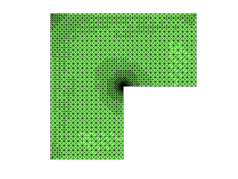
Figure 1: mesh generated by error estimator

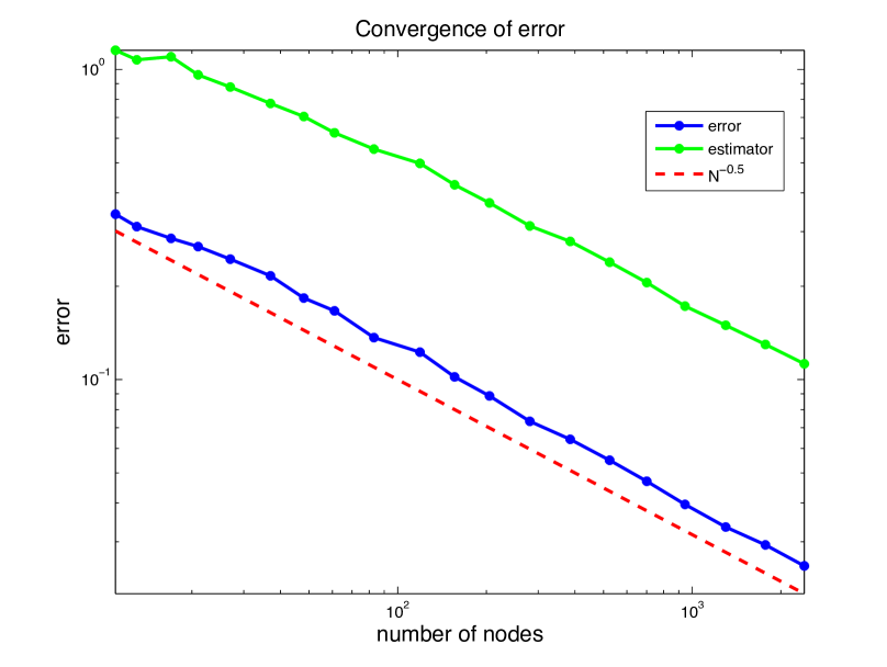
Figure 2: error $\|\mbox{\boldmath$\sigma$}-\mbox{\boldmath$\sigma$}_{h}\|+\|u-u_{h}\|$ and estimator

Mesh generated by $\eta$ is shown in Figure 6.1. The refinement is mainly around the reentrant corner. Comparison of the true error and the $\eta$ is shown in Figure 6.2. Moreover, the slope of the log(dof)- log(error) for the $\eta$ and the true error is $-1/2$, which indicates the optimal decay of the error with respect to the number of unknowns.

References

- [1] M. Ainsworth and J. T. Oden, A Posteriori Error Estimation in Finite Element Analysis, John Wiley & Sons, Inc., 2000.
- [2] A. Aziz, R. Kellogg, and A. Stephens, Least-squares methods for elliptic systems, Math. Comp., 44 (1985), 53-70.
- [3] P. B. Bochev and M. D. Gunzburger, Least Squares Finite Element Methods, Springer, Berlin, 2009
- [4] P. B. Bochev and M. D. Gunzburger, On least-squares finite element methods for the Poisson equation and their connection to the Dirichlet and Kelvin principles, SIAM J. Numer. Anal., 43:1 (2005), 340-362.
- [5] D. Boffi, F. Brezzi, and M. Fortin, Mixed Finite Element Methods and Applications, Springer Series in Computational Mathematics, 44, Springer, 2013.
- [6] D. Braess, Finite Elements: Theory, Fast Solvers and Applications in Solid Mechanics, 3rd edition, Cambridge University Press, Cambridge, UK, 2007.
- [7] J. H. Bramble, R. D. Lazarov, and J. E. Pasciak, A least-squares approach based on a discrete minus one inner product for first order system, Math. Comp., 66 (1997), 935-955.
- [8] Z. Cai, R. Lazarov, T.A. Manteuffel and S.F. McCormick, First-order system least squares for second-order partial differential equations: part I., SIAM J. Numer. Anal., 31 (1994), 1785-1799.
- [9] Z. Cai, T.A. Manteuffel and S.F. McCormick, First-order system least squares for second-order partial differential equations: Part II, SIAM J. Numer. Anal., 34:2 (1997), 425–454.
- [10] Z. Cai, T.A. Manteuffel, S.F. McCormick, and J. Ruge, First-order system LL* (FOSLL*) for scalar partial differential equations, SIAM J. Numer. Anal., 39 (2001), 1418-1445.
- [11] Z. Cai and Ku, Optimal error estimates for the div least-squares method with data f in L2 and application to nonlinear problems, SIAM J. Numer. Anal., 47:6 (2010), 4098-4111.
- [12] J. M. Cascon, R. H. Nochetto, and K. G. Siebert, Design and convergence of afem in H(div), Math. Models and Methods in Applied Sciences, 17(2007), 1849-1881.
- [13] P. G. Ciarlet, The Finite Element Method for Elliptic Problems, North-Holland, Amsterdam, 1978.
- [14] D. C. Jespersen, A least-square decomposition method for solving elliptic systems, Math. Comp., 31 (1977), 873-880.
- [15] B. N. Jiang, The Least-Squares Finite Element Method: Theory and Applications in Computational Fluid Dynamics and Electromagnectics, Spring, Berlin, 1998.
- [16] A. I. Pehlivanov, G. F. Carey, and R. D. Lazarov, Least squares mixed finite elements for second order elliptic problems, SIAM J. Numer. Anal., 31 (1994), 1368-1377.
- [17] P. A. Raviart and J. M. Thomas, A mixed finite element method for 2-nd order elliptic problems, Mathmatical Aspects of Finite Element Methods, Lecture Notes in Mathematics, #606, I. Galligani and E. Magenes, eds., Springer-Verlag, New York, 1977, 292-315.
- [18] R. Verfürth, A Review of A-Posteriori Error Estimation and Adaptive Mesh Refinement Techniques, John Wiley and Teubner Series, Advances in Numerical Mathematics, 1996.
- [19] R. Verfürth, A Posteriori Error Estimation Techniques for Finite Element Methods, Oxford Numerical Mathematics and Scientific Computation, Oxford University Press, 2013.