The Role Model Estimator Revisited

Abstract

We re-visit the role model strategy introduced in an earlier paper, which allows one to train an estimator for degraded observations by imitating a reference estimator that has access to superior observations. We show that, while it is true and surprising that this strategy yields the optimal Bayesian estimator for the degraded observations, it in fact reduces to a much simpler form in the non-parametric case, which corresponds to a type of Monte Carlo integration. We then show an example for which only parametric estimation can be implemented and discuss further applications for discrete parametric estimation where the role model strategy does have its uses, although it loses claim to optimality in this context.

I Preamble

In 2008, I submitted a short semi-technical paper [1] to the IT transactions on the occasion of James L. Massey’s $75^{th}$ birthday. One aim of the paper was to please Jim who often expressed his liking for conceptual papers with simple technical content. Although the paper was dropped for reasons that will become apparent, it achieved its aim of pleasing Jim who repeatedly commented positively on the paper in the years before he passed away. I would speculate that Jim also liked the pun on the “role model” metaphor in the paper mirrorring our relationship as past student to PhD advisor.

The present paper re-visits the ideas presented in [1] and brings a fresh perspective on the subject. In the following section, we will introduce and discuss the role model strategy. Section III shows how the solution of the role model convex program reduces to Monte Carlo integration in the non-parametric case, a much simpler technique well known in the Bayesian community. This realization is the reason why the original paper project [1] was dropped. Section IV discusses the parametric case, where the role model strategy may be of use after all, and why its relevance was not immediately obvious because we operate in the domain of discrete probability mass functions where parametric estimation is not normally considered. An example involving the constraint node operation in a factor graph based SUDOKU solver is presented where parametric estimation is useful, and other potential applications are discussed.

II Introduction and the Role Model Estimator

The role model framework introduced in [1] is illustrated in Figure 1.

Figure 1: The Role Model Framework

The discrete random variables $X_{k}$, $Y_{k}$ and $Z_{k}$ form a Markov chain for every $k$. In the following, we drop the time index $k$ when not essential as our source and channels are assumed to be memoryless. The role model estimator is the optimal estimator for $X$ given the observation $Y$, which provides for every observation $Y=y$ the full a-posteriori probability mass function $P_{X|Y=y}$ over the domain of $X$. Our aim is to train an estimator for $X$ using the random variable $Z=z$, which is labeled “estimator in training” in the figure. The output of this estimator is labeled $Q_{X|Z=z}$ to reflect the fact that it is not necessarily the true a-posteriori probability mass function of $X$ given the observation $Z=z$, but an approximation thereof. The estimator in training is Bayesian optimal if $Q_{X|Z=z}=P_{X|Z=z}$ for every $P_{Z}(z)>0$.

The reason why $P_{X|Z=z}$ is not available directly may be that the channel $P_{Z|Y}$ is unknown, or that the channel $P_{Z|Y}$ is known but that the resulting exact computation of $P_{X|Z=z}$ is too complex for practical use. The particularity of the role model framework, in contrast to more complicated estimation frameworks such as those where the EM and similar algorithms operate, is that we have access to the role model estimator and to its output to help design the estimator in training. This brings up the justified question of why we don’t just use the role model estimator directly instead of training an estimator based on $Z$. This may have several reasons:

• the observations $Y_{k}$ and the resulting a-posteriori distributions $P_{X|Y=y}$ may only be available during a training phase but not when our estimator goes live;

• the observations $Y_{k}$ may only be available intermittently and our estimator in training is required to fill the gaps at times $k$ when $Y_{k}$ is not available;

• the computation of $P_{X|Y=y}$ may be too costly and only feasible offline during a simulation, or online intermittently for the purpose of training the estimator $Q_{X|Z=z}$.

We will later discuss a few technical examples in the context of iterative decoding and communication receivers where these conditions are fulfilled. [1] gives hypothetical general examples outside the domain of communications where this scenario could also be of interest.

What we call the role model strategy consists in aiming to minimize the expected divergence between the a-posteriori distribution $P_{X|Y=y}$ computed by the role model estimator, and the distribution-valued heuristic output $Q_{X|Z=z}$ of the estimator in training, i.e., to seek the $Q_{X|Z=z}$ for every $z$ that minimizes

$$ED(P_{X|Y}||Q_{X|Z})\stackrel{{\scriptstyle\mathrm{def}}}{{=}}\sum_{z}\sum_{y}P(yz)D(P_{X|Y=y}||Q_{X|Z=z}),$$

where we use the notation $ED(.||.)$ as in [2] to signify the expected information divergence, where expectation is always taken on the joint distribution of the conditioning variables. The averaging required to compute this expression may be impractical, and hence we use the law of large numbers and the fact that all our processes are ergodic to state

$$ED(P_{X|Y}||Q_{X|Z})=\lim_{N\rightarrow\infty}\frac{1}{N}\sum_{k=1}^{N}D(P_{X|Y_{k}=y_{k}}||Q_{X|Z_{k}=z_{k}}),$$ (1)

and approximate the quantity to be minimized by a time average of the divergence between the two distribution-valued outputs of our estimators. Note that this may look like a frequentist/empirical approach, but we are at no point counting frequencies here, so the divergences being averaged are true divergences. It is only the average divergence that becomes an approximation if we perform the time averaging over a finite time interval of length $N$ rather than taking the limit as $N$ goes to infinity. We note that $ED(P_{X|Y}||Q_{X|Z})$ is convex in $Q_{X|Z}$, and hence the set of distributions $Q_{X|Z=z}$ for every $z$ that we need can be sought using numerical convex optimization techniques.

We devised the role model strategy as a heuristic approach to address this type of scenario. We had no expectation that this strategy could be optimal. The divergence that is minimized cannot in general be reduced to zero, unless $Z$ is a sufficient statistic for $Y$ with respect to $X$, which is never the case in the applications of interest. Hence, this is not a system identification problem, where the estimator in training eventually models the role model. It therefore came as a surprise when we realized that the following holds:

Theorem 1 (The “role model” theorem)

If $X$, $Y$ and $Z$ form a Markov chain $X-Y-Z$, then

$$ED(P_{X|Y}||Q_{X|Z})=H(X|Z)-H(X|Y)+ED(P_{X|Z}||Q_{X|Z}).$$

In particular,

$$ED(P_{X|Y}||Q_{X|Z})\geq H(X|Z)-H(X|Y)$$

with equality if and only if $Q_{X|Z=z}=P_{X|Z=z}$ for all $z$ such that $P(z)>0$.

The theorem shows that the minimization we suggested converges to the optimal solution $Q_{X|Z}=P_{X|Y}$. Hence, by imitating the role model, we converge to the best solution given our degraded observations, despite the fact that the role model we seek to imitate has better observations. The proof of the theorem is trivial and given in [1]. Note that the theorem requires the Markov property. A similar-looking result can be shown when the Markov property does not hold by stating the identity

$$\sum_{xyz}P(yz)P(x|yz)\log\frac{P(x|y)}{Q(x|z)} = ED(P_{X|Z}||Q_{X|Z})$$

$$+H(X|Z)-H(X|Y),$$

effectively showing that $Q_{X|Z}=P_{X|Z}$ minimizes the expression on the left, but this expression is only equal to $ED(P_{X|Y}||Q_{X|Z})$ when the Markov condition is verified.

It should be stressed that the appellation “theorem” was chosen for this result not on the basis of its mathematical intricacy, which it clearly lacks, but on the basis of its conceptual counter-intuitiveness (from the author’s perspective) and central role it was thought to have in the applications under consideration. In the following section, we will show that the role model strategy reduces to a much simpler form that is well known in the Bayesian estimation community, after discussing a class of applications and their constraints. The role model strategy will regain some meaning in the last section of the paper, where we show a class of applications where the simpler method does not apply but where the role model strategy remains a valid approach.

III The Non-Parametric Case and Monte Carlo Integration

Initial interest for the scenario described was born out of efforts to design optimal post-processing procedures for sub-optimal components in iterative decoders. In the min-sum approximation of the sum product algorithm for decoding low-density parity-check (LDPC) codes, the optimal Bayesian operation under independence assumption in the constraint nodes of the decoder is replaced by a sub-optimal operation as illustrated in Figure 2.

Figure 2: The min-sum approximation for LDPC decoders

In the figure, the incoming observations $Y_{1},Y_{2},Y_{3}$ are aggregated from channel observations during previous decoder iterations and are assumed independent, as is common practice in the design of belief propagation algorithms. In this case, the role model estimator, expressed as a mapping of log-likelihood ratios, is given by

$$L(X|\underline{Y})=2\tanh^{-1}\left(\prod_{i}\tanh\frac{L(X|Y_{i})}{2}\right),$$

which is a fairly complex scalar function of multiple variables often considered too costly for implementation, while the estimator in training is a function $Q_{X|Z=z}$ of

$$Z=\left(\min_{i}|L(Y_{i})|,\prod_{i}\mbox{sign}L(Y_{i})\right).$$

For this simple binary case, the optimal post-processing $P_{X|Z=z}$ can be computed analytically [3] under Gaussian assumption and is fairly simple to compute when the variances of all incoming observations are identical. However, as soon as we deviate from this case, i.e., when the incoming observations have different variances as is the case for irregular LDPC codes, or if we wish to go beyond the Gaussian simplifying assumption, $P_{X|Z=z}$ becomes very difficult to compute. Hence the role model approach allows us to use numerical optimization algorithms to train a post-processing function to converge to the optimal estimator by running the sum-product rule and the estimator-in-training in parallel offline during a simulation, and then using the resulting low-complexity estimator online in the device (e.g., a mobile handset). Another potential practical scenario consists in running both estimators in parallel in the device for a limited time while training the low complexity estimator, then shutting off the more complex estimator to save energy and conserve battery time. Note that the random variable $Z$ in this example is continuous but scalar. A fairly accurate estimator can be trained by quantizing $Z$ finely and computing a lookup table of the a-posteriori distributions of $X$ for each quantized value of $Z$.

We will now show that, for this non-parametric approach that aims to estimate the a-posteriori distributions of $X$ for all values of $Z$, the role model strategy reduces to a much simpler method well known in the Bayesian community as a case of Monte Carlo integration.

For now, let us approach the optimization problem via the time-averaging formulation (1) where we operate on a finite block length and drop the limit for simplicity. It is easy to see that the minimization with respect to the matrix $Q_{X|Z}(x|z)$ for all $x$ and $z$ that we require simplifies to separate maximizations for each individual $z$ of the type

$$\begin{cases}\max_{Q(.|z)}&\sum_{k:z_{k}=z}\sum_{x}P(x|y_{k})\log Q(x|z)\\ \text{subj.~{}to}&\sum_{x}Q(x|z)=1\\ &Q(x|z)\geq 0,\forall x\end{cases}$$

We now take the liberty of ignoring the inequality constraints and setting up the Lagrange conditions rather than the KKT conditions, because the solution will show that there is no danger of any variables becoming negative. For any $z$, we obtain by differentiating with respect to $Q(x|z)$

$$\sum_{k:z_{k}=z}\frac{P(x|y_{k})}{Q(x|z)}=\lambda$$

and hence

$$Q(x|z)=\lambda^{-1}\sum_{k:z_{k}=z}P(x|y_{k}).$$

The normalization condition requires that $\lambda=|\{k:z_{k}=z\}|$ and the solutions clearly satisfy $Q(x|z)\geq 0$ since they are obtained as an average of probabilities.

We conclude that the solution of the role model strategy for any $z$ in the time averaging case is simply the time average of the a-posteriori distributions computed by the role model for all $Y_{k}$ such that $Z_{k}=z$. Again, we insist that this is not simply a frequentist/empirical approach as may appear. The quantities being added here are not numbers of occurrences but true Bayesian a-posteriori distributions computed by the role model. The correct training for our estimator of $X$ for the symbol $z$ is to average the distribution-valued estimations of the role model componentwise over the time instances when $z$ is observed.

Although we showed this for finite $N$, it is easy to see that the same holds in the limit as $N$ goes to infinity, and hence for the expectation $ED(P_{X|Y}||Q_{X|Z})$. An alternative view is that the optimal strategy is to evaluate the sum

$$P(x|z)=\sum_{y}P(x|y)P(y|z)=E_{P_{Y|Z=z}}[P(X|Y)]$$

as a time average, as briefly stated in [4].

In the min-sum algorithm discussed above, and in any similar applications where it is possible to adapt the full $|\mathcal{Z}|\times|\mathcal{X}|$ parameter set for $Q_{X|Z}$, the role model strategy is an overkill and Monte Carlo integration gives the same solution by elementary averaging without resorting to complicated numerical convex optimization methods. In the next section, we will see that there is still a niche for the role model strategy when the full parameter set is too large for practice.

IV The Parametric Case: an Example

When the full parameter set is not available, Monte Carlo integration is not an option and the role model strategy becomes a possibly interesting approach. While this is easy to state, it is not an obvious proposition because we don’t tend to think of parametric estimation for discrete random variables. Indeed, we are not proposing to constrain the conditional probability mass functions $Q_{X|Z}$ to be parametric distributions in the sense that a Gaussian density is a parametric probability density function. Rather, as we will see in our examples, there are scenarios where the domain $\mathcal{Z}$ of $Z$ makes it impractical to estimate an a-posteriori model $Q_{X|Z=z}$ for every possible $z$. In such scenarios, we may be constrained to using a parametric function of $Z$, i.e., $Q_{X|Z=z}=f_{\alpha}(z)$. In such a case, the role model strategy loses its optimality as the space of possible functions $f_{\alpha}(.)$ will not in general include the mapping that makes $Q_{X|Z}$ converge to $P_{X|Z}$. Hence, the role model strategy in this context is a purely heuristic approach that may or may not exhibit advantages or weaknesses with respect to other heuristic optimization criteria and can be judged solely on the basis of its numerical performance.

An early example applying the role model strategy in a semi-parametric manner was described in [5] for a hypothetical rank-based message-passing decoder for non-binary LDPC codes. In fact, a more pertinent question than that studied in [5] would be to design post-processing operations for the suboptimal operations in the Extended Min-Sum (EMS) algorithm [6], a reduced complexity version of the sum-product algorithm for non-binary LDPC codes. However, the EMS algorithm is quite a difficult construct to understand, so that a full study of parametric post-processing, while practically relevant, would obscure rather than clarify matters in the context of this paper. Hence, we have chosen to treat an alternative example of lesser practical relevance but that is easier to understand.

The example is the use of graph-based decoding for solving soft SUDOKU puzzles. We omit an introduction to universally known SUDOKU puzzles and refer the reader to [7] for futher details and definitions. By “soft” SUDOKU, we mean puzzles that receive general noisy observations of the correct entries in the grid rather than observations that are either correct or erased. Observations for every entry in the grid are available as a-posteriori probability mass functions over the 9-ary alphabet using a known and accurate channel model. SUDOKU puzzles can be represented as a factor graph where every one of the 81 variables is connected to 3 constraints and every constraint (9 rows, 9 columns and 9 subgrids) involves 3 variables. The factor graph of a $4\times 4$ SUDOKU defined over the alphabet $\{1,2,3,4\}$ is represented in Figure 3.

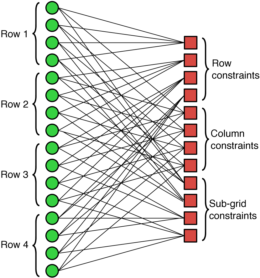
Figure 3: The factor graph of a $4\times 4$ SUDOKU solver

Our interest in the context of this paper is for the operation in the constraint nodes. Constraint nodes receive 9 a-posteriori observations of their participating variables, which we assume to be independent in line with common practice in belief propagation algorithms. The constraint node’s task is to return to each variable its a-posteriori probability given the observations of the remaining 8 variables in the constraint. Let us denote by $\mathbf{M}=[m_{ij}]$ the $9\times 9$ matrix of incoming messages into a constraint node, where

$$m_{ij}=P(X_{i}=j|\underline{Y}_{i})$$

where $\underline{Y}_{i}$ generically denotes the set of channel observations that led to the incoming message on the $i$-th branch into the constraint node. It is clear that the probability that the first variable in the constraint has value $j$, given observations of the other 8 variables, is the sum of probabilities of all configurations of the other 8 variables that don’t include the value $j$. If we denote by $\mathbf{M}_{\setminus ij}$ the matrix $\mathbf{M}$ with its $i$-th row and $j$-th column removed, we can state that an outgoing message component from the constraint node can be expressed as

$$m^{\prime}_{ij}=\operatorname{perm}(\mathbf{M}_{\setminus ij})$$

where $\operatorname{perm}(\mathbf{A})$ denotes the Cauchy permanent [8] of the matrix $\mathbf{A}$. The permanent is a patently difficult function to compute and the best algorithms known compute an approximation of the permanent in probabilistically polynomial time, which polynomial is considerably larger than $n!$ for sizes $n$ of interest to us. We can hence assume that $8!=40320$ operations are needed to compute the permanent above. This is a large number of operations for every node at every iteration of a belief propagation solver, but well within the range of offline simulation, so a perfect testing ground for our role model strategy. We can now try to replace the permanent computation by any approximation and use the role model strategy to design post-processing functions for the approximation.

For example, we can opt to do the following:

• take the 3 largest elements in each row of $\mathbf{M}$ and replace the remaining entries by a uniform distribution adding to the same sum to obtain the matrix $\mathbf{M^{\prime}}$,

• re-write the matrix $\mathbf{M^{\prime}}$ as $\mathbf{H}+\mathbf{T}$ where $\mathbf{T}$ contains uniform rows whose values are consistent with the uniform tails produced in the previous step, and $\mathbf{H}$ contains the non-uniform values minus the uniform tail value for those head entries not in the tails, and zero where the tail entries of $\mathbf{M^{\prime}}$ are;

• we now approximate the required permanent as

  $$\operatorname{perm}\mathbf{M}_{\setminus ij}\approx\operatorname{perm}\mathbf{H}_{\setminus ij}+\operatorname{perm}\mathbf{T}_{\setminus ij}$$

• we compute the elements of the outgoing matrix using this approximation and normalize the rows so they sum to 1 and look like true probability mass functions.

This is much easier to compute because $\mathbf{H}$ is sparse and $\mathbf{T}$ has uniform rows, but it is a very poor approximation because the permanent of a sum of matrices is not at all well approximated by the sum of their permanents. Figure 4 shows the EXIT chart of a factor-graph based SUDOKU solver, where the two red curves correspond to the optimal and sub-optimal constraint node operations, and the blue curves correspond to the constraint node operations for various channel signal to noise ratios (SNR).

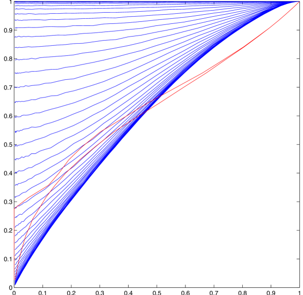
Figure 4: EXIT chart of a SUDOKU solver using the optimal and approximate constraint node operations

Surprisingly, the red curves are not too far apart in particular in the top half of the EXIT chart, indicating that despite the very rough approximation we are using, the result is sufficiently informative to achieve acceptable performance, and the full complexity permanent computation should only be used in the early iterations.

Now for the application of the role model strategy. The observations for our role model postprocessor in this case consist of the rows of the outgoing matrix computed using the permanent approximations. The observation space is the set of 9-ary probability distributions. This is a continuous space and is no longer scalar like in the binary min-sum case. Hence, we cannot simply quantize it finely in order to apply Monte Carlo integration and converge to the optimal a-posteriori estimation. What we can do, however, is to apply arbitrary transformations to the probability vectors. For example, we can take replace the sum $\operatorname{perm}\mathbf{H}+\operatorname{perm}\mathbf{T}$ by a weighted sum $\alpha_{i}\operatorname{perm}\mathbf{H}+(1-\alpha_{i})\operatorname{perm}\mathbf{T}$ and optimize the weights $\alpha_{i}$. Hence the problem becomes one of finding the best parameters $\alpha_{i}$ to optimize the solver performance. The problem is that solver performance itself is difficult to measure and can only be optimized by exhaustive search algorithm. The role model strategy in this case yields a tracktable convex optimization procedure where $ED(P_{X|Y}||Q_{X|Z})$ is the optimization metric. $P_{X|Y}$ here is the correct a-posteriori distribution obtained with the true permanent, and $Q_{X|Z}$ is the $\alpha_{i}$-corrected result of the sum of permanents approximation. Note that with this approach, we have lost any claim of optimality, and anyone who prefers another metric over ours is entitled to do so. The only valid criterion for comparing metrics is simulated performance of the resulting optimized solvers.

V Conclusion

We have described the role model strategy as a convex program whose solution is the Bayesian optimal estimator in training. We showed that the strategy reduces to Monte Carlo integration in the non-parametric case, and discussed the parametric case with an example where the strategy can be used but Monte Carlo integration would not work.

In fact, applications of post-processing optimization for sub-optimal estimators are burgeoning in the literature and many metrics have been proposed for optimizing the post-processing stage of, say, the EMS algorithm for non-binary LDPC codes, demodulators for Bit-Interleaved Coded Modulation (BICM) and many others. Some, such as [9] claim theoretical motives for their approaches, while others, such as [10], are self-declaredly heuristic in their approach. Given our analysis so far and the fact that these are all parametric models, we tend to agree with the latter.

References

- [1] J. Sayir, “What makes a good role model,” 2008, arXiv pre-print. [Online]. Available: http://arxiv.org/abs/0809.1300
- [2] T. M. Cover and J. A. Thomas, Elements of Information Theory. Wiley, New York, 1991, no. ISBN 0-471-24195-4.
- [3] G. Lechner and J. Sayir, “Improved sum-min decoding of LDPC codes,” in Proc. Int. Symp. Inf. Theory and Its App. (ISITA), Parma, Italy, Oct. 2004.
- [4] J. Sayir, “EXIT chart approximations using the role model approach,” in Proc. IEEE Int. Symp. Inform. Theory (ISIT), Jun. 2010. [Online]. Available: http://arxiv.org/abs/1006.0659
- [5] ——, “Design of non-binary decoders using the role model framework,” in Proc. Int. Symp. on Turbo Codes & Rel. Topics, Brest, France, Sep. 2010.
- [6] D. Declercq and M. P. Fossorier, “Decoding algorithms for nonbinary LDPC codes over GF(q),” IEEE Trans. Commun., vol. 55, no. 4, pp. 633–643, Apr. 2007. [Online]. Available: http://publi-etis.ensea.fr/2007/DF07”
- [7] “Sudoku,” article in Wikipedia. [Online]. Available: http://en.wikipedia.org/wiki/Sudoku
- [8] “Permanent,” article in Wikipedia. [Online]. Available: http://en.wikipedia.org/wiki/Permanent
- [9] T. T. Nguyen and L. Lampe, “Bit-interleaved coded modulation with mismatched decoding metrics,” IEEE Trans. Commun., vol. 59, no. 2, pp. 437–447, feb 2011.
- [10] L. Szczecinski, “Correction of mismatched l-values in bicm receivers,” IEEE Trans. Commun., vol. 60, no. 11, pp. 3198–3208, nov 2012.