Stochastic modeling of cargo transport by teams of molecular motors

Abstract

Many different types of cellular cargos are transported bidirectionally along microtubules by teams of molecular motors. The motion of this cargo-motors system has been experimentally characterized in vivo as processive with rather persistent directionality. Different theoretical approaches have been suggested in order to explore the origin of this kind of motion. An effective theoretical approach, introduced by Müller et al. Mueller2008 , describes the cargo dynamics as a tug-of-war between different kinds of motors. An alternative approach has been suggested recently by Kunwar et al. Kunwar , who considered the coupling between motor and cargo in more detail.
Based on this framework we introduce a model considering single motor positions which we propagate in continuous time. Furthermore, we analyze the possible influence of the discrete time update schemes used in previous publications on the system’s dynamic.

1 Introduction

In the last years bidirectional motion along microtubules was observed in many different cell types Welte2004 ; Steinberg2004 . In most of these cells it is still not clear how this bidirectional motion is realized.

Similar to a human road network connecting different places, the cell provides several filaments which can be used for directed transport. Besides the transport utility, the filaments give the cell its characteristic shape. To achieve this double goal the cell produces a cortex of filaments close to the membrane and radial growing filaments from the nucleus to the periphery. The set of these filaments constitutes the cytoskeleton. Intracellular transport along microtubules, which is a radial growing filament, is managed by mainly two kinds of transporters, the so-called molecular motors which are identified as kinesin and dynein Hirokawa . The principal difference between the two kinds of motors is their preferred walking direction. The microtubules are polarized, i.e. they have well-defined directions which are called plus- and minus-direction, respectively. Kinesin’s preferred orientation is to the plus-end of the microtubule, while dynein’s orientation is opposed. Assuming that microtubules mainly grow with their plus end to the cell periphery cellular cargos can be moved to the nucleus and to the membrane by dynein and kinesin, respectively. However, secretory cargos which could be thought to leave the cell as fast and straight as possible, actually show a saltatory motion in vivo Trinczek . This behavior suggests that a number of cellular cargos exists, on which kinesins as well as dyneins are bound at the same time. One possible reason for this motion is to pass obstacles by a second try Dohner . The detailed mechanisms, which are leading to this unconventional bidirectional motion are for most of the motor-cargo systems still unknown.

To describe this bidirectional motion theoretically two mechanisms have been suggested: The first one assumes that $N_{+}$ kinesins and $N_{-}$ dyneins are involved in a mechanical tug-of-war and fight for the direction the cargo effectively moves, while the second one requires a control mechanism to achieve coordinated in vivo-behavior Gross2002 ; Welte1998 . The pure tug-of-war model was introduced by Müller et al. Mueller2008 to describe lipid droplet movement in evolving Drosophila embryo cells. They use a mean-field model, meaning that the motors of one team share the load equally. As a consequence, all kinetic quantities are determined by the number of attached motors to the filament. Indeed, since the motors can bind to and unbind from the filament, the number of motors of each kind attached to the filament fluctuates between zero and $N_{\pm}$ with time. Between two attachment/detachment events, the cargo’s velocity is constant and determined by the strength of the two teams (which depends on the number of attached motors). The number of attached motors also determines the load force felt by each team of motors, and exerted by the opposite team via the cargo. Once one motor detaches one observes a cascade of detachments of motors of this kind and therewith it is possible, in the framework of this model, to generate motility states with high velocity, where one team wins over the other.

This model is quite elegant since experimental observables like the cargo’s velocity can be calculated analytically. However, since this walking in concert was not yet observed in vitro, Kunwar et al. had a closer look at different observables, like the pausing time and run length of single trajectories but did not find matching results in experiments. Therefore they introduced a model taking explicitly the motor positions into account and models the motor-cargo coupling as a linear spring.

In this contribution, we introduce a general model with simple reaction rates which propagates the cargo along its equation of motion in continuous time. Furthermore, we compare and discuss the consequences of using different update schemes.

2 Model

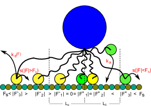
Figure 1: Sketch of the model dynamics. Two kind of motors: one team prefers to walk to the plus-end (green) while the other prefers walking to the minus-end (yellow) of a microtubule. Within the region $L_{0}$ around the cargo’s center of mass the motors apply no force on the cargo (blue).

Inspired by the bidirectional cargo transport models of Mueller2008 ; Kunwar we define a stochastic model to move a cargo by teams of molecular motors along a microtubule. $N_{+}$ and $N_{-}$ motors are tightly bound to the cargo and pull it in plus- and minus-direction, respectively. In contrast to Mueller2008 and in agreement with Kunwar we take every single motor position $x_{i}$ into account and calculate the thereby generated force $F_{i}$ on the cargo. We model the motor tail, which permanently connects the motor head to the cargo, as linear spring with an untensioned length $L_{0}$ and a spring constant $\alpha$. In contrast to Müller’s model Mueller2008 where the motors can attach (with rate $k_{a}$) to and detach from the filament (with force-dependent rate $k_{d}(F_{i})$) only, in our model the motors can once bound to the filament, a one-dimensional infinite lattice, can make a step of size $d$ with a force-dependent rate $s(F_{i})$. Since it seems to be biological relevant that the motors feel no force when they attach to the filament we reduce the allowed attachment region to $\pm L_{0}$ around the center of mass of the cargo.

Due to the de-/attaching events the number $n_{\pm}$ of plus (minus) motors bound to the filament is in the range $0\leq n_{+}\leq N_{+}$ ($0\leq n_{-}\leq N_{-}$). The resulting force on the cargo at position $x_{C}(t)$ at time $t$ is then given by the sum of all single forces

$$F (x_{C}(t),\{x_{i}\})=\sum_{i=1}^{n_{+}+n_{-}}F_{i}(x_{C}(t),\{x_{i}\})$$

$$= \sum_{i=1}^{n_{+}+n_{-}}\alpha\bigg{[}\Big{(}(x_{i}-x_{C}(t))-L_{0}\mathop{\mathrm{sgn}}(x_{i}-x_{C}(t))\Big{)}\cdot\Theta\big{(}|x_{C}(t)-x_{i}|-L_{0}\big{)}\bigg{]},$$

with the Heaviside step function $\Theta(.)$. In this paper we illustrate how we extend the model of Kunwar et al. for a continuous time propagation of the cargo in the case of the simple relations for the stepping and detachment rates introduced in Mueller2008 and given below.

The motors cannot stand arbitrarily high forces. Thus the so-called stall force $F_{S}$ gives the maximal force under which a motor can walk in its preferred direction. We split the stepping rate $s(F_{i})$ in two regimes: (I) forces smaller in absolute value than the stall force ($|F_{i}|<F_{S}$) where the motors walk in their preferred direction and (II) forces bigger in absolute value than the stall force ($|F_{i}|\geq F_{S}$) where the motors walk opposed to their preferred direction and use

$$s(|F_{i}|)=\begin{cases}\frac{v_{f}}{d}\Big{(}1-\frac{|F_{i}|}{F_{S}}\Big{)}\ \ \ \ |F_{i}|<F_{S}\\ \\ \frac{v_{b}}{d}\Big{(}1-\frac{|F_{i}|}{F_{S}}\Big{)}\ \ \ \ |F_{i}|<F_{S}\end{cases}$$ (2)

with $v_{b}\ll v_{f}$ Carter ; Mallik2005 .
Assuming that the motors can walk on several close microtubules in a crowded environment and that their attachment point to the cargo is not necessarily the same, a sterical exclusion of the motor heads on the lattice is not regarded in the model.

For the detachment rate we use Mueller2008

$$k_{d}(|F_{i}|)=k_{d}^{0}\exp\left(\frac{|F_{i}|}{F_{D}}\right),$$ (3)

with the force-free detachment rate $k_{d}^{0}$ and the detachment force $F_{D}$, which determines the force scale.

Update mechanisms

In the mean-field model Mueller2008 the cargo moves with a constant velocity during two motor events, calculated by the number of attached motors of each team. The time at which the next event occurs, is calculated by means of Gillespie’s algorithm Gillespie . Within this framework the cargo’s velocity is piecewise linear.
Kunwar et al. Kunwar use a parallel, thus discrete time update scheme to propagate the system. At every fixed time step $\Delta t$ they calculate the probability that a motor event occurs within this time step. An event should be rare within $\Delta t$ to get a good approximation of the the exact solution in continuous time. In their simulations they use $\Delta t=10^{-6}$ s.
Once the motor dynamic is determined, one has to decide how the cargo reacts to each change in the motor configuration. In Kunwar two different cargo dynamics are introduced: either the cargo moves instantaneously to the position with balanced forces, or it undergoes a viscous force from the environment. The mean-field model of Mueller2008 was treated in the case of an instantaneously reacting cargo.

In Kunwar a viscous environment was taken into account by calculating the position of a cargo with radius $R$ after $\Delta t$ according to

$$x_{C}(t+\Delta t)=x_{C}(t)+\sum_{i=1}^{n_{+}+n_{-}}\frac{F_{i}}{6\pi\eta R},$$ (4)

where $\eta$ is the fluid’s viscosity.

To get a more general approach we rather use the cargo’s equation of motion

$$m\frac{\partial^{2}x_{C}(t)}{\partial t^{2}}=-\beta\frac{\partial x_{C}(t)}{\partial t}+\sum_{i=1}^{n_{+}+n_{-}}F_{i}(x_{C}(t),\{x_{i}\}),$$ (5)

with $\beta=6\pi\eta R$ and the cargo’s mass $m$, to determine the time-dependent position of the cargo.

By determining the force applied on each motor by the distance between motor head position and the center of mass of the cargo, the force $F_{i}$ depends on time, too. Hence, the motor rates for stepping and detaching are time-dependent. Thus the cargo moves in a viscous medium in a harmonic potential of the sum of the springs. Note that the number of engaged springs changes, if the distance between a motor and the cargo falls below or exceeds $L_{0}$. Therefore we have to solve eq. (5) piecewise on segments with a constant number of motors which pull the cargo. On every single segment we solve the equation

$$m\frac{\partial^{2}x_{C}(t)}{\partial t^{2}}=-\beta\frac{\partial x_{C}(t)}{\partial t}-\epsilon x_{C}(t)+\epsilon\zeta,$$ (6)

with

$$\epsilon=\sum_{i=1}^{n_{+}+n_{-}}\alpha\cdot\Theta\big{(}|x_{C}(t)-x_{i}|-L_{0}\big{)}$$ (7)

which determines the effective spring constant and

$$\zeta=\sum_{i=1}^{n_{+}+n_{-}}\big{(}x_{i}-\mathop{\mathrm{sgn}}(x_{C}(t)-x_{i})L_{0}\big{)}\cdot\Theta\big{(}|x_{C}(t)-x_{i}|-L_{0}\big{)},$$ (8)

the effective potential generated by the given motor configuration. We then get the cargo position $x_{C}(t)$ at time $t$ on the segments with constant number of pulling motors

$$x_{C}(t)=\frac{\lambda_{1}\zeta+\lambda_{1}x_{0}-v_{0}}{\lambda_{1}-\lambda_{2}}\exp(\lambda_{2}t)+\frac{v_{0}-\lambda_{2}\zeta-\lambda_{2}x_{0}}{\lambda_{1}-\lambda_{2}}\exp(\lambda_{1}t)-\zeta$$ (9)

with

$$\lambda_{1}=-\frac{\beta}{2m}+\sqrt{\left(\frac{\beta}{2m}\right)^{2}-\frac{\epsilon}{m}}\ \ \ \ \text{ and }\ \ \lambda_{2}=-\frac{\beta}{2m}-\sqrt{\left(\frac{\beta}{2m}\right)^{2}-\frac{\epsilon}{m}}.$$ (10)

Now knowing the cargo position at an arbitrary time $t$ we can use Gillespie’s algorithm for time-dependent rates Gillespie_1978 to calculate the next event time.

3 Results

Log-log plot of the normalized count of times between two occurring events calculated by the exact algorithm Gillespie_1978 for $F_{S}=2$ pN (blue) and $F_{S}=6$ pN (red). Obviously, times between events smaller than $10^{-6}$ s occur for both stall forces.

At first we analyze the distribution of times between two motor updates which we generate with the exact algorithm and the parameter set given in Table LABEL:paraset.

In Fig. 3 the normalized count of times between events is shown in a double logarithmic plot. Obviously, times smaller than $\Delta t=10^{-6}$ s occur if we propagate the system with the exact algorithm. By analyzing $10^{5}$ events we calculated the mean time between events $\langle t\rangle$ for the two stall forces as well as the smallest $t_{s}$ and the longest time $t_{l}$ between two events and get

$$F_{S}=2 \ \ \ \langle t\rangle=3.5\cdot 10^{-3}\text{ s}\ \ \ t_{s}=3.1\cdot 10^{-8}\text{ s}\ \ \ t_{l}=1.8\cdot 10^{-1}\text{ s}$$ pN

$$F_{S}=6 \ \ \ \langle t\rangle=1.8\cdot 10^{-3}\text{ s}\ \ \ t_{s}=1.6\cdot 10^{-8}\text{ s}\ \ \ t_{l}=8.1\cdot 10^{-2}\text{ s}.$$ pN

It remains the question how this influences the system’s observables. In Kunwar the focus is on the run length and pause duration of the single walks. However, as the motion is stepwise, these observables are defined from quite arbitrary time/distance thresholds. That is why we prefered to concentrate on another quantity to compare our data to the parallel update scheme, namely the discrete velocity

$$\tilde{v}=\frac{|x(t+\text{D}t)-x(t)|}{\text{D}t},$$ (11)

where we use $\text{D}t=0.16$ s as it was suggested in Mueller2008 .

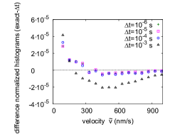
(a)

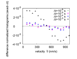
(b)

Fig. 2: Difference between the exact velocity histogram generated with Gillespie’s algorithm Gillespie_1978 and the parallel update scheme suggested in Kunwar with different $\Delta t$ for (a) $F_{S}=2$ pN and (b) $F_{S}=6$ pN. Sample size per histogram: $5\cdot 10^{6}$.

In Fig. 2 we show the difference between the normalized velocity histogram generated by Gillespie’s algorithm Gillespie_1978 and those generated by the parallel update scheme for different $\Delta t$ and for two different stall forces $F_{S}$. In both cases an increase in $\Delta t$ increases the cargo’s velocity as shown in Table 2.

		$\Delta t$
$F_{S}$	exact	$10^{-6}$ s	$10^{-5}$ s	$10^{-4}$ s	$10^{-3}$ s
2 pN	149.0	149.8	149.7	150.3	155.4
	$\pm$0.10	$\pm$ 0.05	$\pm$ 0.05	$\pm$ 0.08	$\pm$ 0.08
6 pN	449.4	450.2	450.4	451.1	458.5
	$\pm$0.18	$\pm$0.09	$\pm$0.13	$\pm$0.13	$\pm$0.13

Table 2: Mean discrete velocity $\langle\tilde{v}\rangle$ in nm/s for the exact and the parallel update.

4 Discussion

We have introduced in this contribution an exact algorithm to propagate the motors-cargo system in continuous time.

An analysis of the times between two events reveals that very different time scales are involved: while most times between two events are greater than $10^{-3}$ s, a fraction of events are separated by less than $10^{-7}$ s.

From our results, a first conclusion is that if one uses parallel update, the time step $\Delta t$ should at least be less than $10^{-5}$ s to expect results in good agreement with the continuous time dynamics. However, the continuous time dynamics reveals that much shorter time scales are involved, as a signature of cascades of events. These cascades are overlooked in the discrete updates even for time steps as small as $\Delta t=10^{-6}$ s. While we have found that this approximation does not alter the quality of measurements of most quantities when such a small time step is used (as it is the case in Kunwar ), one cannot exclude that for some other sets of parameters, and/or for more sensitive observables, these cascades could have a stronger effect. Actually, though further numerical support should be provided to conclude, our results seem to indicate that discrete updates systematically slightly underestimate the probability to have weak cargo velocities (unless prohibitively small time steps would be used). This can be understood as an effect of the synchronization of the motors induced by the time discretization, similarly to what happens with the mean-field assumption used in Mueller2008 (which can also be seen as a synchronization mechanism) which overemphasizes large velocity states. As a conclusion, in such a system involving very different time scales, an exact algorithm in continuous time provides an efficient numerical scheme: it allows to avoid any possible artefact that would come from the discretization, without any extra numerical cost.

In further work we will extend this model to more realistic motor rates and show for biologically relevant parameter sets how some external quantity like the ATP concentration or the viscosity of the surrounded fluid can control the drift of the cargo Klein2014 .

- [1] N. J. Carteret al. Nature, 435(7040):308–312, 05 2005.
- [2] K. Döhner et al. Trends in microbiology, 13(7):320–327, 2005.
- [3] D. T. Gillespie. Journal of Computational Physics, 22(4):403–434, 12 1976.
- [4] D. T. Gillespie. Journal of Computational Physics, 28(3):395–407, 9 1978.
- [5] S. P. Gross et al. The Journal of Cell Biology, 156(4):715–724, 2002.
- [6] N. Hirokawa et al. Current Opinion in Cell Biology, 10(1):60–73, 2 1998.
- [7] A. Kunwar et al. Proceedings of the National Academy of Sciences, 108(47):18960–18965, 2011.
- [8] R. Mallik et al. Current Biology, 15(23):2075–2085, 12 2005.
- [9] M. J. I. Müller et al. Proceedings of the National Academy of Sciences, 105(12):4609–4614, Mar. 2008.
- [10] G. Steinberg et al. Journal of Microscopy, 214(2):114–123, 2004.
- [11] B. Trinczek et al. J Cell Sci, 112 ( Pt 14):2355–2367, Jul 1999.
- [12] M. A. Welte. Current Biology, 14(13):R525–R537, 7 2004.
- [13] M. A. Welte et al. Cell, 92(4):547–557, 2 1998.
- [14] S. Klein, C. Appert-Rolland, and L. Santen. In preparation.