Adequate bases of phase space master integrals for $gg\to h$ at NNLO and beyond

Abstract

We study master integrals needed to compute the Higgs boson production cross section via gluon fusion in the infinite top quark mass limit, using a canonical form of differential equations for master integrals, recently identified by Henn, which makes their solution possible in a straightforward algebraic way. We apply the known criteria to derive such a suitable basis for all the phase space master integrals in afore mentioned process at next-to-next-to-leading order in QCD and demonstrate that the method is applicable to next-to-next-to-next-to-leading order as well by solving a non-planar topology. Furthermore, we discuss in great detail how to find an adequate basis using practical examples. Special emphasis is devoted to master integrals which are coupled by their differential equations.

1 Introduction

In order to study the compatibility of the assumed Higgs particle discovered by ATLAS and CMS Aad:2012tfa ; Chatrchyan:2012ufa with the standard model precise theoretical predictions are required. One of the basic physical observables is the total inclusive Higgs production cross section which is, as is well known, dominated by gluon fusion at the LHC. For a long time the state of the art in fixed-order perturbative calculations of the total inclusive Higgs production cross section in the gluon fusion channel has been next-to-leading-order (NLO) for electroweak corrections and next-to-next-to-leading order (NNLO) for QCD corrections (see ref. Dittmaier:2011ti for comprehensive reviews). The latter ones have firstly been calculated in the infinite top mass limit Harlander:2002wh ; Anastasiou:2002yz ; Ravindran:2003um while finite mass corrections were included in refs. Marzani:2008az ; Harlander:2009bw ; Pak:2009bx ; Harlander:2009mq ; Pak:2009dg ; Harlander:2009my .

In recent years, various next-to-next-to-next-to-leading order (N³LO) QCD approximations have become available Moch:2005ky ; Bonvini:2014jma but the full calculation remains a challenging frontier. Some partial results have been obtained with full dependence on the partonic center-of-mass energy (in the infinite top mass limit), including the three-loop matrix elements Baikov:2009bg ; Gehrmann:2010ue ; Gehrmann:2010tu , the one-loop squared single-real-emission contributions Anastasiou:2013mca ; Kilgore:2013gba and the convolutions of NNLO cross sections with splitting functions Hoschele:2012xc ; Buehler:2013fha ; Hoeschele:2013gga which require the knowledge of the NNLO master integrals to higher orders in $\epsilon$ Pak:2011hs ; Anastasiou:2012kq . Other results are only available as threshold expansions. They include the partonic cross section of the purely three-parton real emission Anastasiou:2013srw , the two-loop soft current Duhr:2013msa ; Li:2013lsa , the one-loop two emission contribution Li:2014bfa , culminating in the hadronic Higgs production cross section at threshold Anastasiou:2014vaa .

In this paper we calculate the dependence of master integrals, appearing in calculations of the total inclusive Higgs production cross section via gluon fusion in the infinite top mass limit, on the kinematic variable $x$, which is derived by the method of differential equations Kotikov:1990kg ; Kotikov:1991pm ; Bern:1993kr ; Remiddi:1997ny ; Gehrmann:1999as (see refs. Argeri:2007up ; Smirnov:2012gma for comprehensive reviews). The differential equations become, however, more and more complicated with growing loop order. At N³LO level it seems rather difficult to obtain solutions of the differential equations high enough in the $\epsilon$-expansion in a naively chosen basis of master integrals. Recently, a very elegant form of differential equations was introduced in ref. Henn:2013pwa which is supposed to exist at any loop order. This conjecture has been strengthened by plenty of examples at two-loop Henn:2013pwa ; Henn:2013woa ; Argeri:2014qva ; Henn:2014lfa ; Caola:2014lpa ; Gehrmann:2014bfa and three-loop order Henn:2013tua ; Henn:2013nsa ; Caron-Huot:2014lda which show the applicability to various kinematic configurations, even to single-scale integrals Henn:2013nsa . Although there exist algorithms for constructing an adequate basis in cases of differential equations depending on $\epsilon$ polynomially Argeri:2014qva and for finite integrals in $D=4$ dimensions Caron-Huot:2014lda as well as a strategy for the construction from a basis with a triangular finite part of the homogeneous differential equation matrix Gehrmann:2014bfa , a general algorithm to find such a basis is still missing. However, a lot of methods, tricks and ideas do exist which are discussed in the references above and used in practice.

The purpose of this paper is twofold. On the one hand, we review the techniques for finding an adequate basis using NLO and NNLO master integrals for Higgs production cross section in sections 2 and 3, respectively, giving the explicit bases as well. We also present a trick using a characteristic form of higher order differential equations for the case of coupled master integrals in section 3.2, which, to our knowledge, has hitherto not been discussed in the literature. On the other hand, we show the applicability of the method to the state of the art problem of finding solutions with full $x$-dependence to master integrals appearing in N³LO Higgs production by solving a non-planar topology in section 4. In section 5 we state our conclusions and outlook.

2 General idea and NLO warm-up

2.1 Reduction to master integrals

Suppose that we have families of Feynman integrals, also called topologies, to be evaluated where the propagator labelled by $i$ is raised to a power $a_{i}$, usually called index. Within dimensional regularization 'tHooft:1973mm integration-by-parts (IBP) identities give linear relations among integrals with different values of indices $a_{i}$ Chetyrkin:1981qh . Starting from a large set of values of $a_{i}$, all integrals can be reduced to a linearly independent set of master integrals by making use of the IBP identities by means of, e.g., Laporta algorithm Laporta:2001dd .

We treat phase space integrals contributing to the Higgs production cross section as cut integrals Cutkosky:1960sp . In the same way as loop integrals, cut integrals can be reduced to master integrals via IBP identities by means of the reverse-unitarity method Anastasiou:2002yz ; Anastasiou:2013srw . The only difference stems from the fact that integrals containing a cut line with a non-positive index $a_{c}\leq 0$ vanish. In order to identify subtopologies, families of Feynman integrals obtained by setting subsets of indices to be zero, that have no cuts or are scaleless within dimensional regularization, we use the private Mathematica package TopoID. This code also provides symmetries useful for the reduction and allows us to identify a minimal set of master integrals.

In this work, we have used an in-house implementation of Laporta algorithm, as well as the program FIRE Smirnov:2008iw ; Smirnov:2013dia together with its unpublished C++ version. The result is stored in a reduction table for later repeated use.

In the reduction, we use Feynman propagators in Euclidean metric, which applies also to the master integrals given in this paper.

2.2 Differential equations for master integrals

In the case of Higgs production via gluon fusion in the infinite top mass limit, each topology has only one massive Higgs line and we have forward scattering kinematics, i.e., the incoming partons’ momenta $p_{1}$ and $p_{2}$ are equal to the outgoing partons’ momenta $p_{3}=p_{1}$ and $p_{4}=p_{2}$, respectively. Therefore, aside from the trivial overall mass scale, the integrals depend only on one kinematic variable $x=m_{h}^{2}/s$ with $s=(p_{1}+p_{2})^{2}$ and the space-time dimension $D=4-2\epsilon$. Without loss of generality we can set $s=1$. The derivative of each master integral with respect to $x$ is given, up to a constant prefactor, by raising the index of the massive line by one and the resulting integral can be reduced to a linear combination of master integrals. In this way, we arrive at a set of differential equations for $N$ master integrals, which can be expressed as the following matrix form:

$$\partial_{x}\tilde{f}(x,\epsilon)=\tilde{A}(x,\epsilon)\tilde{f}(x,\epsilon),$$ (1)

where $\tilde{f}$ is a column vector of master integrals of length $N$ and $\tilde{A}$ is an $N\times N$ matrix.

2.3 Change of basis

The choice of master integrals is not unique and one can always choose another basis of master integrals. The basis transformation can be obtained by looking up the entries in the reduction table for the new basis integrals $f$ which are by construction linear combinations of the old basis integrals $\tilde{f}$:

$$f(x,\epsilon)=B(x,\epsilon)\tilde{f}(x,\epsilon),$$ (2)

with an $N\times N$ matrix $B$. Taking the derivative of eq. (2) with respect to $x$, one arrives at the differential equations for the new basis integrals:

$$\partial_{x}f(x,\epsilon)=A(x,\epsilon)f(x,\epsilon),\qquad\text{with }A:=\left[(\partial_{x}B)+B\tilde{A}\right]B^{-1}.$$ (3)

This means that, providing an alternative basis $f$, we instantly know the form of its differential equation $A$ by use of the reduction table to obtain $B$ as well as $\tilde{A}$.

2.4 Master integral basis in canonical form

Following Henn’s conjecture Henn:2013pwa , a basis $f$ of integrals exists in which all master integrals become so-called pure functionsand satisfy the differential equations

$$\partial_{x}f(x,\epsilon)=\epsilon\bar{A}(x)f(x,\epsilon),$$ (4)

i.e., the dependence of the matrix $A$ on the dimensional parameter $\epsilon$ is factored out as $A=\epsilon\bar{A}$. To ensure the basis integrals are pure functions, $\bar{A}$ should have the form

$$\bar{A}(x)=\sum_{k}\frac{\alpha_{k}}{x-x_{k}},$$ (5)

where $x_{k}$ are constants and $\alpha_{k}$ are constant matrices. The system of differential equations (4) can be expanded in $\epsilon$ as

$$\partial_{x}f^{[n]}(x)=\bar{A}(x)f^{[n-1]}(x),\qquad\text{with}\quad f(x,\epsilon)=\sum_{n=-\infty}^{\infty}\epsilon^{n}f^{[n]}(x),$$ (6)

and one can solve it order by order. The expanded system (6) is triangular in the sense that only lower order functions $f^{[n-1]}$ appear in the right-hand side of the set of differential equations for $f^{[n]}$, hence the solution can be easily obtained in terms of iterated integrals, provided the boundary condition is fixed at some point $x=x_{0}$.

The matrix $\bar{A}$ respects singular points of the process, in this case we have: for $x=0$ the Higgs line becomes massless and additional infra-red singularities may be introduced. In addition, at $x=1$, more precisely for approach from $x<1$, the diagrams develop a non-zero imaginary part, since the Higgs may be produced indeed. In our calculation, we observe another singular point at $x=-1$ for some NNLO integrals, yielding the canonical form (5) for the differential equations:

$$\bar{A}(x)=\frac{a}{x}+\frac{b}{1-x}+\frac{c}{1+x},$$ (7)

where we find the matrices $a$, $b$ and $c$ to just contain rational numbers. This assures that at any order the $\epsilon$-expansion of the solution of the differential equations are iterated integrals expressible as harmonic polylogarithms (HPLs) Remiddi:1999ew , which can be easily manipulated with HPL package implemented in Mathematica Maitre:2005uu ; Maitre:2007kp . The first term of the solution in the expansion is a constant, the next in general contains also HPLs of weight one, the next in addition HPLs of weight two, etc. Therefore, the result will be a linear combination of HPLs with constant prefactors. If the integration constants have suitable weight the master integrals are pure functions.

2.5 Parametric representations of integrals

Although there is no algorithm to obtain an optimal basis from arbitrary basis integrals in general, there exist some guiding principles how to find candidate integrals that may give a canonical form. For example, integrals having unit leading singularities ArkaniHamed:2010gh ; Cachazo:2008vp are expected to be uniform weight functions. Another one is investigating parametric representations of integrals, which is described as follows.

The notion that pure functions are built from iteratively integrated logarithms Henn:2013pwa imposes strong constraints on the candidates. Sketching the Feynman parameter representation for an integral $I$ (see, e.g., Smirnov:2012gma )

$$I(x,\epsilon) \sim\int\prod_{j}d\alpha_{j}\frac{\left[U(\{\alpha_{i}\})\right]^{e_{U}}\prod_{i}\alpha_{i}^{a_{i}-1}\delta(\sum_{k}\alpha_{k}-1)}{\left[W(x,\{\alpha_{i}\})\right]^{e_{W}}},$$

$$e_{U} =a-(l+1)D/2,$$

$$e_{W} =a-lD/2,$$

$$a =\sum_{i}a_{i},$$ (8)

where $l$ is the number of loops, $U$ and $W$ are polynomials in the Feynman parameters $\alpha_{i}$ and $a_{i}$ are the corresponding indices. An integral of form

$$\int\prod_{j}d\alpha_{j}\frac{1}{\left[g(\{\alpha_{i}\},x)\right]^{k}},\qquad\text{with }k\in\mathbb{N},$$ (9)

where $g$ is an irreducible polynomial, is favored over those of different form as it yields more likely a pure function in $x$, see the discussion about d-log forms in ref. Henn:2013wfa .

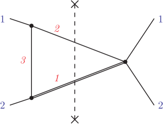
Figure 1: The NLO topology $\text{TNLO}_{2}(a_{1},a_{2},a_{3})$. The massive Higgs line is depicted by a double line, whereas the dashed line denotes the cut. Numbers in roman indicate the incoming and outgoing momenta $p_{1}$ and $p_{2}$, and numbers in italic label the propagators according to the corresponding indices.

Let us illustrate this statement by considering the NLO problem. After applying symmetries of diagrams and performing partial fraction decomposition, one is left with only one topology $\text{TNLO}_{2}(a_{1},a_{2},a_{3})$ depicted in fig. 1. A standard Laporta algorithm finds one master integral, typically given by TNLO₂(1,1,0) obeying the differential equation

$$\partial_{x}\text{TNLO}_{2}(1,1,0)=-\frac{1-2\epsilon}{1-x}\text{TNLO}_{2}(1,1,0).$$ (10)

Although the missmatch from eq. (4) can be cured with a suitable $x$-normalization (see section 3), let us try to understand it from the parametric representation eq. (2.5). We have $U=1$ from the $\delta$-function for all NLO integrals. Furthermore, TNLO₂(1,1,0) has $a=2$ and therefore $e_{W}\approx 0$, where we understand the “$\approx$” symbol as the $D=4$ approximation. Therefore, we find $k\approx 0$ in eq. (9), accounting for the non-canonical form of eq. (10). The other way around, we need $a=3$ to obtain $k=e_{W}\approx 1$. This can be achieved, e.g., by raising the index of the massive Higgs line by one, $\text{TNLO}_{2}(2,1,0)$, or adding another propagator, $\text{TNLO}_{2}(1,1,1)$. In the former case, raising the index of the Higgs line causes an additional $\alpha_{1}$ in the numerator which cancels against an overall $\alpha_{1}$ in $W$ of the denominator. Writing down the differential equations, we see that the mentioned candidates indeed turn out to form canonical bases:

$$\partial_{x}\text{TNLO}_{2}(2,1,0) =\frac{2\epsilon}{1-x}\text{TNLO}_{2}(2,1,0),$$

$$\partial_{x}\text{TNLO}_{2}(1,1,1) =\frac{2\epsilon}{1-x}\text{TNLO}_{2}(1,1,1).$$ (11)

It is important to remember this fact in the following since these diagrams will appear as subgraphs at higher loop order. Performing the same manipulations, i.e. raising one index of a bubble or stretching it into a triangle, for the subgraphs will lead to promising candidates (see ref. Henn:2013tua as well). In general, we observe that there are cases where adding additional lines or raising indices helps. Finally, it is worth mentioning that the arguments given here have made use of the diagrammatic structure of the integrals, but (apart from the $\alpha_{1}$ cancellation mentioned above) not of the explicit structure of the $W$ polynomial in eq. (2.5) and therefore were (almost) independent of the kinematics. Hence, it is not surprising that some of the integrals in canonical bases given in section 3 and section 4 resemble results for similar topologies with different kinematics found in the literature.

3 NNLO: examples and solutions

3.1 Known techniques

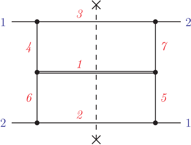
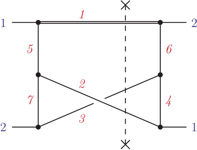
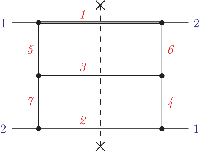
TTA	TTC	TTD
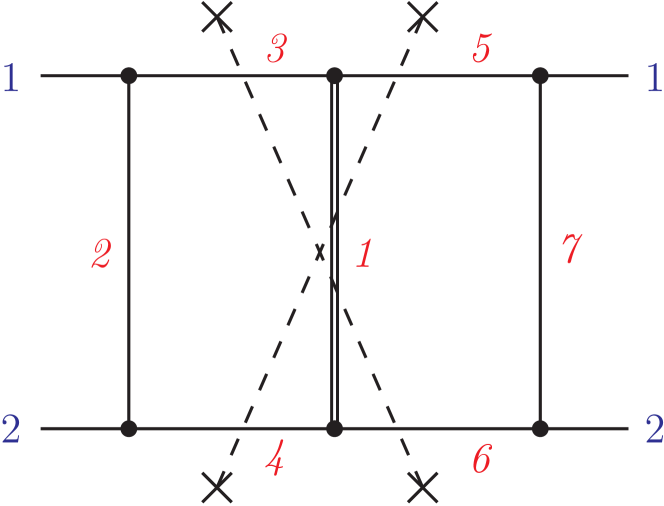
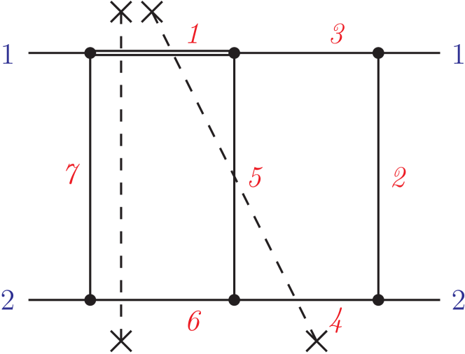
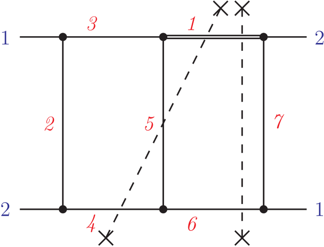
TTE	TTF	TTG
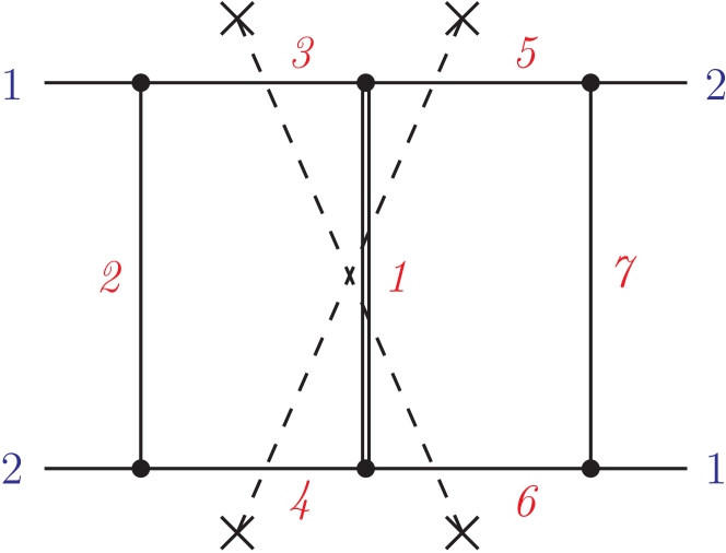
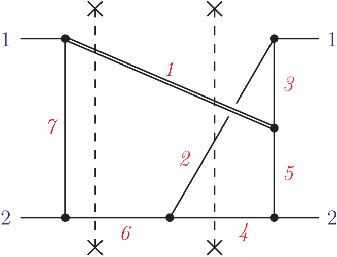
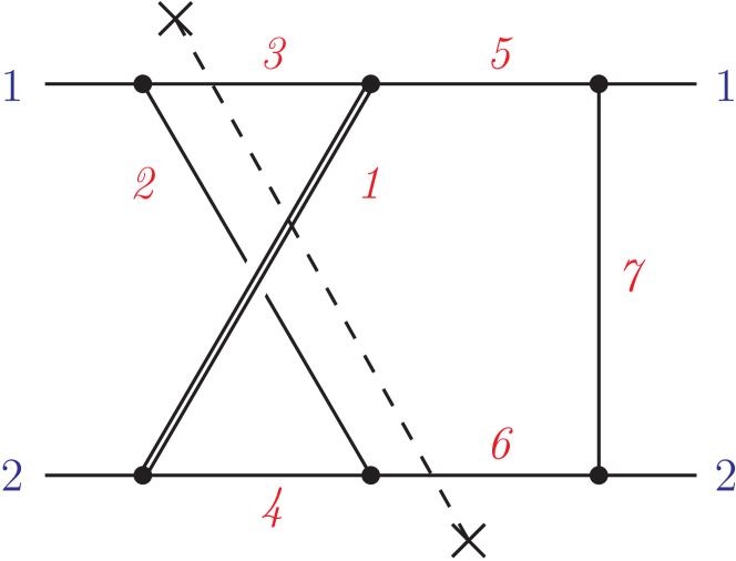
TTH	TTJ	TTK

Figure 2: The NNLO topologies $\text{TT}X_{c}(a_{1},a_{2},a_{3},a_{4},a_{5},a_{6},a_{7})$ involving our choice for a canonical basis. The subscript $c=2,3$ of topologies distinguishes two-particle cuts and three-particle cuts. The massive Higgs line is depicted by a double line, whereas dashed lines denote possible cuts. Numbers in roman indicate the incoming and outgoing momenta $p_{1}$ and $p_{2}$ and numbers in italic label the propagators according to the corresponding indices. In the text we define all integrals as single-cut integrals. For TTE and TTH, two cuts give the same contribution but only one of them is taken into account in the defnition of the corresponding master integrals.

Let us discuss further known tricks for finding an adequate basis by looking at the example of the three-particle phase space diagram defined in terms of the topology $\text{TTA}_{3}$ (see fig. 2) occurring at NNLO via

$$\text{TTA}_{3}(1,1,1,0,0,0,0)=:\text{TTA}_{3}(1,1,1),$$ (12)

where we omit the trailing zeros in the indices for simplicity. In the reduction basis obtained from our reduction table, its differential equation is coupled to another integral $\text{TTA}_{3}(1,1,1,-1,0,0,0)$ having an additional scalar product in the numerator. For the purpose of finding good candidates we raise one index of the massless bubble Henn:2013tua . It is well known that integrating a massless bubble with the indices $b_{1}$ and $b_{2}$ gives, up to a prefactor, a propagator with the index $b_{1}+b_{2}-2+\epsilon$. Therefore, we have

$$V_{1}^{*}=\text{TTA}_{3}(2,2,1)\sim\text{TNLO}_{2}(2,1+\epsilon,0)$$ (13)

and we expect this to be a good candidate from the discussion for the NLO case in section 2. The second candidate which couples to this one can be found by constructing a subtle linear combination. For that purpose, let us compare eq. (2.5) to eq. (9) for $k=1$, i.e. in a first step we set $e_{W}\approx k=1$. This means that we have fixed $a=5$ and $e_{U}\approx-1$. For example the parametric representation of the above candidate $V_{1}^{*}$ is of the type

$$\text{TTA}_{3}(2,2,1) \sim\int\prod_{j}d\alpha_{j}\frac{\alpha_{1}\alpha_{2}\delta(\sum_{k}\alpha_{k}-1)}{\left(\alpha_{1}\alpha_{2}+\alpha_{1}\alpha_{3}+\alpha_{2}\alpha_{3}\right)W(x,\{\alpha_{i}\})}.$$ (14)

One could try $\text{TTA}_{3}(1,2,2)$ which is of the same form, but with $\alpha_{1}\alpha_{2}$ in the numerator replaced by $\alpha_{2}\alpha_{3}$. However, the candidate does not lead to a differential equation of the desired form. Therefore, one can try to identify $W$ in eq. (14) with $g$ in eq. (9), which means we have to cancel the $U$ polynomial $(\alpha_{1}\alpha_{2}+\alpha_{1}\alpha_{3}+\alpha_{2}\alpha_{3})$. This is achieved by adding three integrals to

$$V_{2}^{*}=\text{TTA}_{3}(2,2,1)+\text{TTA}_{3}(2,1,2)+\text{TTA}_{3}(1,2,2)=2\text{TTA}_{3}(2,2,1)+\text{TTA}_{3}(1,2,2).$$ (15)

Note that the construction given above can be generalized to any loop order for this type of sunrise diagrams (see the results of section 4 for the three-loop case).

Constructing the differential equations for the candidates $V_{1}^{*}$ and $V_{2}^{*}$ using eq. (3) we find only $A_{22}$ to be of inappropriate form

$$\lim_{\epsilon\to 0}A=\begin{pmatrix}0&0\\ 0&\frac{1}{1-x}\end{pmatrix}.$$ (16)

The non-vanishing diagonal element corresponds to the homogeneous differential equation of $V_{2}^{*}$ in lowest order in $\epsilon$ and therefore it appears in all orders Argeri:2007up . The problem is resolved by allowing for an $\epsilon$ independent $n(x)$-normalization, i.e. a shift $V_{2}^{*}\to n(x)V_{2}^{*}$, yielding

$$\lim_{\epsilon\to 0}A_{22}=\frac{1}{1-x}+\frac{\partial_{x}n(x)}{n(x)}\overset{!}{=}0.$$ (17)

This determines $n(x)=1-x$ and we have found two elements of the canonical basis

$$V_{1} =\epsilon\text{TTA}_{3}(2,2,1),$$

$$V_{2} =\epsilon(1-x)\bigl{[}2\text{TTA}_{3}(2,2,1)+\text{TTA}_{3}(1,2,2)\bigr{]},$$ (18)

obeying the differential equation with

$$A=\epsilon\begin{pmatrix}-\frac{3}{x}&\frac{1}{x}+\frac{1}{1-x}\\ -\frac{6}{x}&\frac{2}{x}+\frac{4}{1-x}\end{pmatrix}.$$ (19)

The prefactors of $\epsilon$ have been introduced to make the integrals start at finite order.

Note that the result, we have found here, will not be changed by adding more master integrals to the considerations. In this sense, finding a canonical basis can be approached step by step, starting with the integrals with lowest number of lines and continuously increasing that number. Master integrals with coupled differential equations have to be added in one step to the problem, but here other strategies apply, as we show in section. 3.2.

Now we add the next master integral of the topology $\text{TTA}_{3}$ to the problem, given by $V_{3}^{*}=\text{TTA}_{3}(1,1,1,1,0,1,0)$, where we have just taken the integral from the reduction basis as a candidate. Since it has $a=5$ in its parametric representation (2.5), this is a good choice as motivated above. The matrix defining the differential equations becomes

$$A=\begin{pmatrix}-\frac{3\epsilon}{x}&\frac{\epsilon}{x}+\frac{\epsilon}{1-x}&0\\ -\frac{6\epsilon}{x}&\frac{2\epsilon}{x}+\frac{4\epsilon}{1-x}&0\\ -\frac{1}{\epsilon^{2}x}&\frac{1}{2\epsilon^{2}x}&-\frac{2\epsilon}{x}\end{pmatrix},$$ (20)

where the upper left $2\times 2$ block corresponds to $(V_{1},V_{2})$ and forms a canonical basis already as eq. (19). The off-diagonal elements in the last row depend on $\epsilon$ differently from the desired form. These elements correspond to the inhomogeneous terms in the differential equation for $V_{3}^{*}$. The problem is cured by $n(\epsilon)$-normalization, i.e. by changing $V_{3}^{*}\to n(\epsilon)V_{3}^{*}$. In this case we find $n(\epsilon)=\epsilon^{3}$, such that

$$V_{3}=\epsilon^{3}\text{TTA}_{3}(1,1,1,1,0,1,0)$$ (21)

completes a canonical basis of the $3\times 3$ subproblem.

In summary, a diagonal scaling matrix

$$B_{ij}^{\text{s}}=\begin{cases}s_{i}(x,\epsilon),&i=j,\\ 0,&i\neq j,\end{cases}$$ (22)

changes the coefficient matrix as

$$A_{ij}^{\text{s}} =\frac{\partial_{x}s_{i}}{s_{i}}\delta_{ij}+\frac{s_{i}}{s_{j}}A_{ij}.$$ (23)

Lastly, let us remark that bases exist where $\epsilon$ factorizes from their $A$ matrix as in eq. (4) but the matrix is not of the desired form given in eq. (7). For example, choosing

$$V_{3}^{*}=(1+\epsilon)\epsilon^{2}x\text{TTA}_{3}(1,1,1,2,0,1,0)$$ (24)

instead of $V_{3}$ the last row in eq. (20) changes to

$$A=\begin{pmatrix}-\frac{3\epsilon}{x}&\frac{\epsilon}{x}+\frac{\epsilon}{1-x}&0\\ -\frac{6\epsilon}{x}&\frac{2\epsilon}{x}+\frac{4\epsilon}{1-x}&0\\ -3\epsilon&\frac{\epsilon}{2}+\frac{\epsilon}{1-x}&-\frac{2\epsilon}{x}\\ \end{pmatrix},$$ (25)

where the off-diagonal elements in the last row induce non-logarithmic functions in the solution of $V_{3}^{*}$ and therefore the result cannot be a pure function.

3.2 Techniques for coupled master integrals

The techniques we want to discuss next touches on the issue of master integrals coupled by their differential equations. In particular, a problem that occurs frequently is the following: when there is a system of $n$ coupled master integrals in a reduction basis, one tries a set of $n$ candidates for a canonical basis and sees if the resulting $n$ differential equations are of the canonical form or not. Even if one of the $n$ candidates is a good integral that would form a canonical basis with appropriately chosen other $(n-1)$ good integrals, the corresponding differential equation may not be of the canonical form due to a choice of the other $(n-1)$ bad integrals, which makes it difficult to identify good integrals. Nonetheless, it would be worthwhile knowing if one of the $n$ candidates is a canonical basis integral so one could keep good integrals and dismiss bad integrals.

In the following we want to show how to distinguish suitable candidates for canonical master integrals from unsuitable choices using the fact that the system of $n$ coupled first order differential equations is equivalent to one $n$th order differential equation for one of the master integrals. The idea is that the resulting higher order differential equation is unique for each master integral in the sense that it is independent of eliminated integrals. It defines the master integral itself and furthermore takes a specific form for canonical master integrals, founding on the assumption that a set of canonical master integrals exists. Moreover, we will show that once one of canonical master integrals in a coupled system is found the assumption of the existence of a canonical basis allows us to construct a set of the other canonical master integrals coupled to it.

3.2.1 Characteristic form of higher order differential equations

Let us discuss the situation of two coupled master integrals $f_{1}$ and $f_{2}$ to explain the method in detail:

$$f_{1}^{\prime} =a_{11}f_{1}+a_{12}f_{2}+\sum_{i}r_{1i}g_{i},$$

$$f_{2}^{\prime} =a_{21}f_{1}+a_{22}f_{2}+\sum_{i}r_{2i}g_{i},$$ (26)

where primes denote derivatives with respect to $x$ and $g_{i}$ in the right-hand sides are master integrals assumed to be fixed already and to form a canonical basis, obeying

$$g_{i}^{\prime}=\sum_{j}\alpha_{ij}g_{j}.$$ (27)

All the quantities given here depend on $x$ and $\epsilon$. Taking one more derivative with respect to $x$ of the first line of eq. (3.2.1) we find

$$f_{1}^{\prime\prime}=a_{11}^{\prime}f_{1}+a_{11}f_{1}^{\prime}+a_{12}^{\prime}f_{2}+a_{12}f_{2}^{\prime}+\sum_{i}\left(r_{1i}^{\prime}g_{i}+r_{1i}g_{i}^{\prime}\right).$$ (28)

Eliminating $f_{2}$ and $f_{2}^{\prime}$ by eq. (3.2.1) and $g_{i}^{\prime}$ by eq. (27) we obtain a second order differential equation for $f_{1}$:

$$f_{1}^{\prime\prime} =-\left(-a_{11}-\frac{a_{12}^{\prime}}{a_{12}}-a_{22}\right)f_{1}^{\prime}+\left(a_{11}^{\prime}-\frac{a_{11}a_{12}^{\prime}}{a_{12}}+a_{12}a_{21}-a_{11}a_{22}\right)f_{1}$$

$$\quad+\sum_{i}\biggl{(}-\frac{a_{12}^{\prime}r_{1i}}{a_{12}}-a_{22}r_{1i}+a_{12}r_{2i}+r_{1i}^{\prime}+\sum_{j}r_{1j}\alpha_{ji}\biggr{)}g_{i}$$

$$=:-C_{1}f_{1}^{\prime}+C_{0}f_{1}+\sum_{i}C_{0i}g_{i}.$$ (29)

It is important to emphasize that this differential equation is independent of $f_{2}$ and uniquely defines the behaviour of $f_{1}$. The coefficients $C_{1}$, $C_{0}$ and $C_{0i}$ are invariant under any basis transformations that change only $f_{2}$ as $f_{2}\to b_{21}f_{1}+b_{22}f_{2}+\sum_{i}\beta_{2i}g_{i}$.

Case 1: $f_{1}$ and $f_{2}$ are canonical master integrals.

Let us now reveal what characteristic form for the higher order differential equation of $f_{1}$ should appear when $f_{1}$ and $f_{2}$ are canonical master integrals as $g_{i}$ are. In such a basis, $a_{ij}$ and $r_{ij}$ as well as $\alpha_{ij}$ are proportional to $\epsilon$. Therefore, the coefficients $C_{1}$, $C_{0}$ and $C_{0i}$ defined by eq. (29) can be decomposed into $\epsilon$ independent coefficients as

$$C_{1} =C_{1}^{(0)}+\epsilon C_{1}^{(1)},$$

$$C_{0} =\epsilon C_{0}^{(1)}+\epsilon^{2}C_{0}^{(2)},$$

$$C_{0i} =\epsilon C_{0i}^{(1)}+\epsilon^{2}C_{0i}^{(2)},$$ (30)

given by

$$C_{1}^{(0)} =-\frac{a_{12}^{\prime}}{a_{12}},$$

$$C_{1}^{(1)} =\frac{1}{\epsilon}\left(-a_{11}-a_{22}\right),$$

$$C_{0}^{(1)} =\frac{1}{\epsilon}\left(a_{11}^{\prime}-\frac{a_{11}a_{12}^{\prime}}{a_{12}}\right),$$

$$C_{0}^{(2)} =\frac{1}{\epsilon^{2}}\left(a_{12}a_{21}-a_{11}a_{22}\right),$$

$$C_{0i}^{(1)} =\frac{1}{\epsilon}\left(-\frac{a_{12}^{\prime}r_{1i}}{a_{12}}+r_{1i}^{\prime}\right),$$

$$C_{0i}^{(2)} =\frac{1}{\epsilon^{2}}\biggl{(}-a_{22}r_{1i}+a_{12}r_{2i}+\sum_{j}r_{1j}\alpha_{ji}\biggr{)}.$$ (31)

Case 2: $f_{1}$ is a canonical master integral but $f_{2}$ is not.

Even if $f_{2}$ is not a canonical master integral and it makes $a_{ij}$ and $r_{ij}$ not be of canonical form, we can utilize the uniqueness of the coefficients $C_{1}$, $C_{0}$ and $C_{0i}$ in the higher order differential equation for $f_{1}$. They must still have decompositions in $\epsilon$ like eq. (3.2.1), although the identities for $C_{1}^{(m)}$, $C_{0}^{(m)}$, $C_{0i}^{(m)}$ in terms of $a_{ij}$ and $r_{ij}$ eq. (3.2.1) do not hold any longer. Furthermore, it allows us to reconstruct what coefficients $a_{ij}^{\text{p}}$ and $r_{ij}^{\text{p}}$ in a system of differential equations would be within a basis in which $f_{2}$ is properly chosen to be a canonical master integral $f_{2}^{\text{p}}$, under the assumption that such an $f_{2}^{\text{p}}$ does exist. Since in such a proper basis $C_{1}$, $C_{0}$ and $C_{0i}$ take the same form as Case 1 in terms of $a_{ij}^{\text{p}}$ and $r_{ij}^{\text{p}}$, we can invert eq. (3.2.1) to obtain $a_{ij}^{\text{p}}$ and $r_{ij}^{\text{p}}$:

$${a_{12}^{\text{p}}}^{\prime}+C_{1}^{(0)}a_{12}^{\text{p}} =0,$$

$${a_{11}^{\text{p}}}^{\prime}-\frac{{a_{12}^{\text{p}}}^{\prime}}{a_{12}^{\text{p}}}a_{11}^{\text{p}} =\epsilon C_{0}^{(1)},$$

$$a_{22}^{\text{p}} =-a_{11}^{\text{p}}-\epsilon C_{1}^{(1)},$$

$$a_{21}^{\text{p}} =\frac{a_{11}^{\text{p}}a_{22}^{\text{p}}}{a_{12}^{\text{p}}}+\epsilon^{2}\frac{C_{0}^{(2)}}{a_{12}^{\text{p}}},$$

$${r_{1i}^{\text{p}}}^{\prime}-\frac{{a_{12}^{\text{p}}}^{\prime}}{a_{12}^{\text{p}}}r_{1i}^{\text{p}} =\epsilon C_{0i}^{(1)},$$

$$r_{2i}^{\text{p}} =\frac{a_{22}^{\text{p}}r_{1i}^{\text{p}}}{a_{12}^{\text{p}}}-\sum_{j}\frac{r_{1j}^{\text{p}}\alpha_{ji}}{a_{12}^{\text{p}}}+\epsilon^{2}\frac{C_{0i}^{(2)}}{a_{12}^{\text{p}}}.$$ (32)

We can solve this system of differential equations, line by line for $a_{ij}$ and $r_{ij}$, setting the integration constants of $a_{12}$, $a_{11}$ and $r_{1i}$ to constants proportional to $\epsilon$, namely $\epsilon c_{12}$, $\epsilon c_{11}$ and $\epsilon k_{1i}$, respectively.

3.2.2 Construction of canonical basis

Having all entries of $a_{ij}^{\text{p}}$ and $r_{ij}^{\text{p}}$ as in Case 2 of the previous section, one can construct a canonical master integral $f_{2}^{\text{p}}$ that satisfies the differential equations implied by $a_{ij}^{\text{p}}$ and $r_{ij}^{\text{p}}$. The linear basis transformation

$$B=\begin{pmatrix}\mathds{1}&0&0\\ 0&1&0\\ \beta_{2i}&b_{21}&b_{22}\end{pmatrix}$$ (33)

from the basis $(g_{i},f_{1},f_{2})$ obeying the differential equation with the matrix $A$ to the canonical basis $(g_{i},f_{1},f_{2}^{\text{p}})$ with $A^{\text{p}}$ satisfies eq. (3), or

$$B^{\prime}=A^{\text{p}}B-BA,$$ (34)

where the matrix $A$ and $A^{\text{p}}$ are given by

$$A=\begin{pmatrix}\alpha_{ij}&0&0\\ r_{1i}&a_{11}&a_{12}\\ r_{2i}&a_{21}&a_{22}\end{pmatrix},\qquad A^{\text{p}}=\begin{pmatrix}\alpha_{ij}&0&0\\ r_{1i}^{\text{p}}&a_{11}^{\text{p}}&a_{12}^{\text{p}}\\ r_{2i}^{\text{p}}&a_{21}^{\text{p}}&a_{22}^{\text{p}}\end{pmatrix}.$$ (35)

Each component in the row corresponding to $f_{1}$ (the next to the last line) of eq. (34) gives a linear equation for $\beta_{2i}$, $b_{21}$ and $b_{22}$, respectively. The rows above the mentioned one give trivial equations, whereas the row below gives differential equations that serve as consistency checks. Once the basis transformation $B$ is determined, one can obtain an explicit expression of $f_{2}^{\text{p}}$ as a linear combination of $g_{i}$, $f_{1}$ and $f_{2}$.

Note that until the end we do not need to fix the integration constants $c_{12}$, $c_{11}$ and $k_{1i}$ introduced in Case 2. Since from eq. (3.2.1) $a_{12}^{\text{p}}$ is proportional to $c_{12}$ and $a_{21}^{\text{p}}$ and $r_{2i}^{\text{p}}$ are proportional to $c_{12}^{-1}$ whereas $a_{11}^{\text{p}}$, $a_{22}^{\text{p}}$ and $r_{1i}^{\text{p}}$ are independent of it, $c_{12}^{-1}$ can be interpreted as a numerical normalization factor of $f_{2}^{\text{p}}$, see eqs. (22) and (23). In addition to the normalization factor $c_{12}^{-1}$, $c_{11}$ and $k_{1i}$ span a multi-dimensional space of solutions for $f_{2}^{\text{p}}$ and cover the full class of canonical master integrals that are coupled partners to $f_{1}$.

So far, we have seen that if $f_{1}$ is a canonical master integral one can construct another canonical master integral $f_{2}^{\text{p}}$ coupled to $f_{1}$. This leads to an algorithm to see whether $f_{1}$ can be a canonical master integral: assuming $f_{1}$ is a canonical master integral, one tries to construct $f_{2}^{\text{p}}$ on the basis of the above considerations. If it fails at any step, one concludes that $f_{1}$ cannot be a canonical master integral. Once $f_{2}^{\text{p}}$ is explicitly constructed, one can see whether $f_{1}$ and $f_{2}^{\text{p}}$ form a canonical basis as they should, which is equivalent to find a consistent solution of $B$ in eq. (34). The details are as follows:

1. Calculate the coefficients $C_{1}$, $C_{0}$ and $C_{0i}$ in the higher order differential equation for $f_{1}$ from $a_{ij}$ and $r_{ij}$ by eq. (29).

2. Assuming $f_{1}$ is a canonical master integral, one should find that $C_{1}$, $C_{0}$ and $C_{0i}$ have decompositions in $\epsilon$ as eq. (3.2.1), otherwise $f_{1}$ cannot be a canonical master integral and should be dismissed.

3. Reconstruct $a_{ij}^{\text{p}}$ and $r_{ij}^{\text{p}}$ from $C_{1}^{(m)}$, $C_{0}^{(m)}$ and $C_{0i}^{(m)}$ by eq. (3.2.1). If one requires them to be of the desired form

   $$a_{ij}^{\text{p}},r_{ij}^{\text{p}}\sim\epsilon\left(\frac{n_{0}}{x}+\frac{n_{1}}{1-x}+\frac{n_{-1}}{1+x}\right),$$ (36)

   where $n_{0}$, $n_{1}$ and $n_{-1}$ are numbers, the differential equations for $a_{12}^{\text{p}}$, $a_{11}^{\text{p}}$ and $r_{1i}^{\text{p}}$ must be easily solved, and if they are difficult to solve most likely they do not have the above form. If one of the reconstructed entries $a_{ij}^{\text{p}}$ and $r_{ij}^{\text{p}}$ are not of the form eq. (36), $f_{1}$ cannot be a canonical master integral.

4. Find the basis transformation (33) to the basis that satisfies the differential equations given by $a_{ij}^{\text{p}}$ and $r_{ij}^{\text{p}}$ from eq. (34). From this transformation one obtains $f_{2}^{\text{p}}$. If there is no solution of eq. (34) with eq. (33), $f_{1}$ cannot be a canonical master integral.

Note that in our case eq. (36) is imposed on the canonical form, but for the derivation of $f_{2}^{\text{p}}$ we only needed the assumption that $a_{ij}^{\text{p}}$ and $r_{ij}^{\text{p}}$ are proportional to $\epsilon$. Therefore this algorithm should also work for other calculations within the framework of canonical differential equations having different forms (5) in $x$.

3.2.3 Example in the three-particle phase space at NNLO

Let us apply the above algorithm to the example of the two coupled phase space integrals of $\text{TTA}_{3}(a_{1},a_{2},a_{3})$ we have already encountered in section 3.1. More specifically, we put

$$f_{1} =\epsilon\text{TTA}_{3}(2,2,1),$$

$$f_{2} =\text{TTA}_{3}(2,1,1).$$ (37)

We have previously seen that $f_{1}=V_{1}$ is a canonical master integral, nevertheless we will apply the algorithm to this pair of integrals and see what happens. The differential equations have no inhomogeneous terms and therefore

$$r_{1i} =0,$$

$$r_{2i} =0.$$ (38)

Writing down the second order differential equation for $f_{1}$, we can reconstruct $A^{\text{p}}$ from its coefficients:

$$A^{\text{p}}=\epsilon\begin{pmatrix}\frac{c_{11}}{x}+\frac{c_{11}+3}{1-x}&\frac{c_{12}}{x}+\frac{c_{12}}{1-x}\\ -\frac{c_{11}(c_{11}+1)}{c_{12}x}-\frac{(c_{11}+3)(c_{11}-1)}{c_{12}(1-x)}&-\frac{c_{11}+1}{x}-\frac{c_{11}-1}{1-x}\end{pmatrix}.$$ (39)

Correspondingly, we can find $f_{2}^{\text{p}}$ as

$$f_{2}^{\text{p}}=\frac{1-c_{11}(1-4\epsilon)-2\epsilon(1+x)}{c_{12}(1-4\epsilon)}f_{1}-\frac{2\epsilon(1-2\epsilon)(1-3\epsilon)}{c_{12}(1-4\epsilon)}f_{2}.$$ (40)

Once $f_{2}^{\text{p}}$ is obtained, one can easily check that $f_{1}$ and $f_{2}^{\text{p}}$ form a canonical basis with $A^{\text{p}}$.

Note that we have not fixed the integration constants $c_{11}$ and $c_{12}$. As discussed before, $c_{12}$ determines the normalization of $f_{2}^{\text{p}}$. If we choose $c_{11}=-3$ and $c_{12}=1$, $A^{\text{p}}$ turns into eq. (19) and $f_{2}^{\text{p}}$ becomes $V_{2}$, which can be verified by the reduction. Other interesting solutions are given by $c_{11}=1$, $c_{12}=1$ or $c_{11}=-1$, $c_{12}=2$, for which $a_{21}^{\text{p}}=a_{22}^{\text{p}}$ and the second row of $A^{\text{p}}$ becomes independent of $1/(1-x)$ or $1/x$, respectively.

By contrast, if we interchange $f_{1}$ and $f_{2}$ in the above example (3.2.3) and put

$$f_{1} =\text{TTA}_{3}(2,1,1),$$

$$f_{2} =\epsilon\text{TTA}_{3}(2,2,1),$$ (41)

the first coefficient stemming from $C_{1}^{(0)}$ already yields

$$a_{12}^{\text{p}} =-\epsilon c_{12}+\epsilon\frac{c_{12}}{x},$$ (42)

in disagreement with the desired form (36). Therefore we can conclude $f_{1}=\text{TTA}_{3}(2,1,1)$ cannot be a canonical master integral.

3.2.4 Example with a non-zero inhomogeneity

As we will see in section 3.3, there is another pair of coupled integrals $\text{V}_{11}$ and $\text{V}_{12}$ among the NNLO canonical master integrals. Their differential equations contain $V_{1}$ and $V_{2}$ as inhomogeneous terms. Let us apply the algorithm to a basis in which $V_{11}$ is correctly chosen as well as $V_{1}$ and $V_{2}$ but the coupled integral is chosen differently from $V_{12}$. By putting

$$g_{1} =V_{1\phantom{1}}=\epsilon\text{TTA}_{3}(2,2,1),$$

$$g_{2} =V_{2\phantom{1}}=\epsilon(1-x)\left[\text{TTA}_{3}(1,2,2)+2\text{TTA}_{3}(2,2,1)\right],$$

$$f_{1} =V_{11}=\epsilon^{3}\text{TTF}_{3}(1,0,1,1,1,0,1),$$

$$f_{2} =\epsilon^{2}\text{TTF}_{3}(1,0,2,1,1,0,1),$$ (43)

the algorithm gives $A^{\text{p}}$ in the desired form:

$$A^{\text{p}}=\epsilon\left(\frac{a^{\text{p}}}{x}+\frac{b^{\text{p}}}{1-x}\right),$$ (44)

with

$$a^{\text{p}}=\begin{pmatrix}-3&1&0&0\\ -6&2&0&0\\ k_{11}&k_{12}&c_{11}&c_{12}\\ -\frac{c_{11}k_{11}-6k_{12}+2}{c_{12}}&-\frac{2c_{11}k_{12}+2k_{11}+10k_{12}-1}{2c_{12}}&-\frac{(c_{11}+1)(c_{11}+2)}{c_{12}}&-(c_{11}+3)\end{pmatrix},$$ (45)

and

$$b^{\text{p}}=\begin{pmatrix}0&1&0&0\\ 0&4&0&0\\ 0&0&0&0\\ \frac{2(k_{11}-1)}{c_{12}}&-\frac{2k_{11}+4k_{12}-1}{2c_{12}}&\frac{2(c_{11}+2)}{c_{12}}&2\end{pmatrix}.$$ (46)

If we choose the integration constants as

$$c_{12}=1,\qquad c_{11}=-1,\qquad k_{12}=\frac{1}{4},\qquad k_{11}=-1,$$ (47)

we find agreement with the differential equation matrix given in section 3.3, and the reconstructed $f_{2}^{\text{p}}$ turns into $\text{V}_{12}$.

3.2.5 Three or more coupled differential equations

In the case that there are three or more coupled master integrals, one can straightforwardly generalize the arguments in the above. Suppose that one has $n$ coupled master integrals $(n\geq 2)$ to be added into a canonical basis all at once. Starting from the differential equations of order $m$ ($m\geq 1$)

$$f^{(m)}=A^{[m-1]}f,$$ (48)

where the matrix $A^{[m]}$ is recursively defined by

$$A^{[m]}:=\left(A^{[m-1]}\right)^{\prime}+A^{[m-1]}A,\qquad A^{[0]}:=A,$$ (49)

one can obtain the $n$th order differential equation for $f_{i}$ by eliminating $(n-1)$ integrals $f_{j_{1}}$, $f_{j_{2}}$, $\dots$, $f_{j_{n-1}}$ from the system of $n$ differential equations for $f_{i}^{\prime}$, $f_{i}^{(2)}$, …, $f_{i}^{(n)}$. The result has the following form

$$\sum_{m=1}^{n}C_{m}f_{i}^{(m)}=\sum_{k\notin\{j_{1},\dots,j_{n-1}\}}C_{0k}f_{k},$$ (50)

where the summation in the right-hand side is taken for all integrals except the eliminated integrals; in other words, all canonical master integrals already fixed as well as $f_{i}$. The coefficients $C_{m}$ and $C_{0k}$ are given by

$$C_{m}=\frac{\Delta_{mn}}{\Delta_{nn}},\qquad C_{0k}=\frac{\Delta_{k}}{\Delta_{nn}}=\sum_{m=1}^{n}C_{m}A^{[m-1]}_{ik},$$ (51)

where we have normalized $C_{n}$ as unity, $\Delta_{k}=\det(M_{k})$ is the determinant of the following $n\times n$ matrix:

$$M_{k}=\begin{pmatrix}A_{ij_{1}}^{[0]}&\ldots&A_{ij_{n-1}}^{[0]}&A_{ik}^{[0]}\\ \vdots&&\vdots&\vdots\\ A_{ij_{1}}^{[n-1]}&\ldots&A_{ij_{n-1}}^{[n-1]}&A_{ik}^{[n-1]}\end{pmatrix},$$ (52)

and $\Delta_{mn}$ is the cofactor obtained by multiplying $(-1)^{m+n}$ to the determinant of $M_{k}$ with omitting the $m$th row and the $n$th column (hence does not depend on $k$).

Assuming $f_{i}$ is a canonical master integral, one can conclude that the coefficients must have the following structure in $\epsilon$:

$$C_{m} =\frac{\epsilon^{n-1}C_{m}^{(n-1)}+\dots+\epsilon^{n(n+1)/2-m}C_{m}^{(n(n+1)/2-m)}}{\epsilon^{n-1}D^{(n-1)}+\dots+\epsilon^{n(n-1)/2}D^{(n(n-1)/2)}},$$

$$C_{0k} =\frac{\epsilon^{n}C_{0k}^{(n)}+\dots+\epsilon^{n(n+1)/2}C_{0k}^{(n(n+1)/2)}}{\epsilon^{n-1}D^{(n-1)}+\dots+\epsilon^{n(n-1)/2}D^{(n(n-1)/2)}}.$$ (53)

The coefficients $C_{m}$ and $C_{0k}$ are rational functions in $\epsilon$ and thus the set of differential equations for reconstructing the matrix $A^{\text{p}}$, appearing in the basis in which the eliminated integrals $f_{j_{1}}$, $f_{j_{2}}$, $\dots$, $f_{j_{n-1}}$ are properly chosen, becomes quite tedious. However, taking only the leading terms of $C_{m}$ and $C_{0k}$ in $\epsilon$ by replacing $A^{[n]}$ with $A^{(n)}$

$$A^{[n]}_{kl}=A^{(n)}_{kl}+\mathcal{O}(\epsilon^{2}),$$ (54)

may alleviate the complexity of the problem. The first terms of $C_{m}$, i.e., $C_{m}^{(n-1)}/D^{(n-1)}$ give a set of $(n-1)$ differential equations of $(n-1)$ variables $A_{ij_{1}}^{\text{p}}$, $\dots$, $A_{ij_{n-1}}^{\text{p}}$. After solving them, one substitutes the result into the first terms of $C_{0k}$, $C_{0k}^{(n)}/D^{(n-1)}$, which gives a differential equation for $A_{ik}^{\text{p}}$. In this way, one can reconstruct the $i$th row of the matrix $A^{\text{p}}$.

In general, higher order terms of the coefficients in $\epsilon$ expansions are needed to reconstruct the full matrix $A^{\text{p}}$. From a naive counting, $n$ orders of each coefficient have to be taken into account.

Once $A^{\text{p}}$ is completely determined, one can construct the basis transformation $B$ to this basis. The matrix $B$ can be parametrized by filling $(n-1)$ rows corresponding to $f_{j_{1}}$, $\dots$, $f_{j_{n-1}}$ with variables $b_{kl}$. The matrix equation eq. (34) contains derivatives of the variables; however, one does not need to solve any differential equations. Non-trivial equations in $n$ rows of the matrix equation can be solved as follows. Starting with $i$th row, whose components are all zero in the left-hand side, one has a set of linear equations, which can be solved for all variables of a row. Next, one considers this row. On the left-hand side, one can use the chain rule of the derivative and replace derivatives of unsolved variables with the corresponding components of the matrix equation. Then one substitutes the solution for the solved variables. The resulting equations give the next set of linear equations that can determine all variables of another row. Repeating this procedure, one can solve for all the variables by using $(n-1)$ rows, and the remaining row can serve as a consistency check.

The generalized version of the algorithm given in section 3.2.2 that checks whether $f_{i}$ is a canonical master integral is formulated as follows:

1. Derive higher order differential equation for $f_{i}$, i.e. calculate the coefficients $C_{m}$ and $C_{0k}$ given in eq. (51).

2. Check $\epsilon$-dependence of $C_{m}$ and $C_{0k}$, which should be as in eq. (53).

3. Expand $C_{m}$ and $C_{0k}$ in $\epsilon$. Take enough terms to be able to solve for the elements of $A^{\text{p}}$. The differential equations should be solvable by the ansatz eq. (36). In order to proceed, it is enough to find one particular solution for $A^{\text{p}}$.

4. Construct $B$ and check its consistency by use of eq. (34).

If the checks fail at any step, one can conclude $f_{i}$ cannot be a canonical master integral.

Let us conclude with a few final remarks:

• By using the ansatz eq. (36) in solving for the elements of $A^{\text{p}}$, all differential equations appearing in this algorithm can be reduced to algebraic equations.

• In practice $A$ sometimes contains elements equal to zero. Setting the elements at the same positions in $A^{\text{p}}$ to zero may simplify the derivation a lot, provided this additional constraints on the form of $A^{\text{p}}$ gives a solution for $A^{\text{p}}$ and $B$.

• By changing the ansatz eq. (36), the algorithm can be extended to other forms (5) in $x$.

3.3 Canonical master integrals for NNLO Higgs boson production

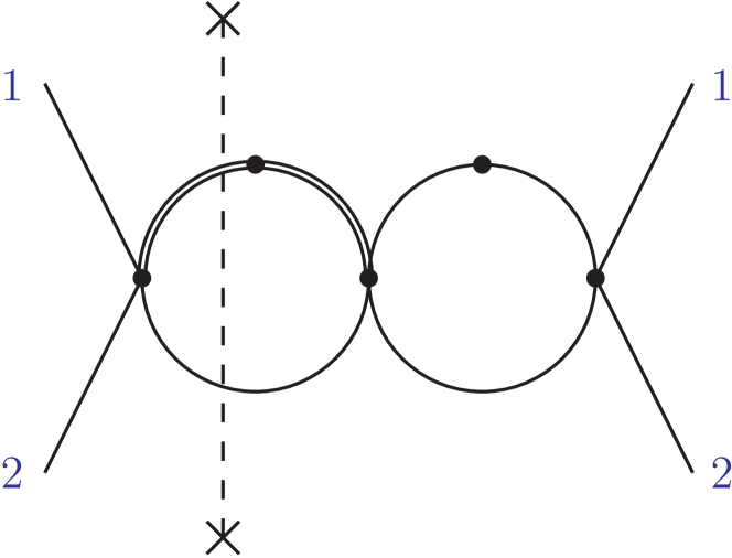
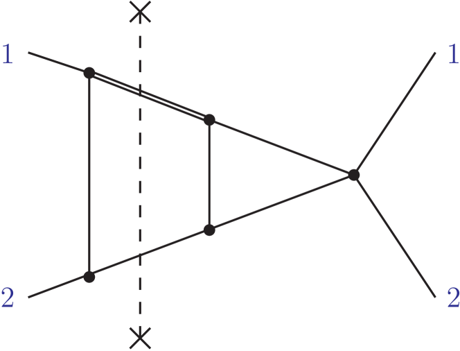
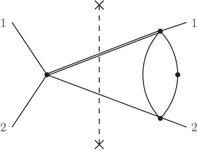
$\text{TTF}_{2}(2,0,2,1,0,1,0)$	$\text{TTF}_{2}(1,0,1,1,1,1,1)$	$\text{TTF}_{2}(1,2,0,0,1,1,0)$
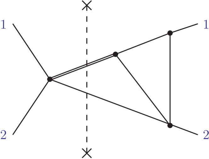
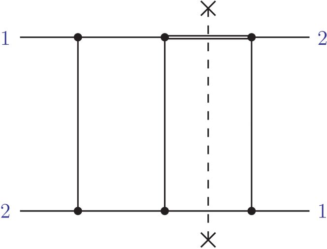
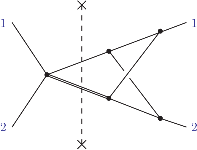
$\text{TTF}_{2}(1,1,1,0,1,1,0)$	$\text{TTG}_{2}(1,1,1,1,1,1,1)$	$\text{TTJ}_{2}(1,1,1,1,1,1,0)$

Figure 3: Two-particle cut diagrams appearing in our choice of canonical master integrals at NNLO.

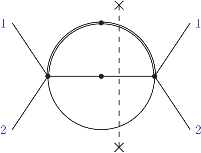
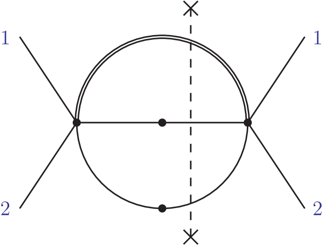
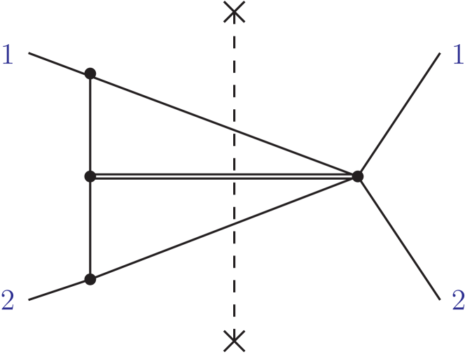
$\text{TTA}_{3}(2,2,1,0,0,0,0)$	$\text{TTA}_{3}(1,2,2,0,0,0,0)$	$\text{TTA}_{3}(1,1,1,1,0,1,0)$
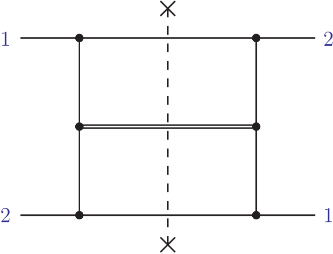
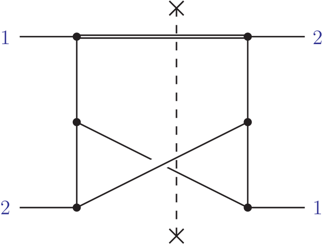
$\text{TTA}_{3}(1,1,1,1,1,1,1)$	$\text{TTC}_{3}(1,2,1,0,1,1,0)$	$\text{TTC}_{3}(1,1,1,1,1,1,1)$
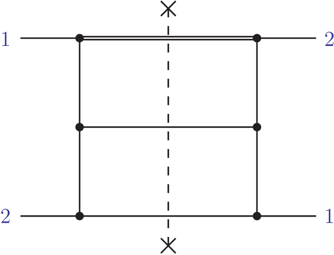
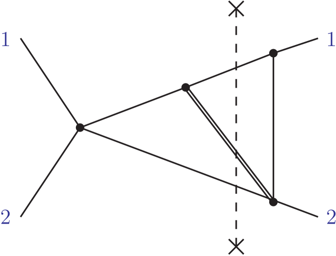
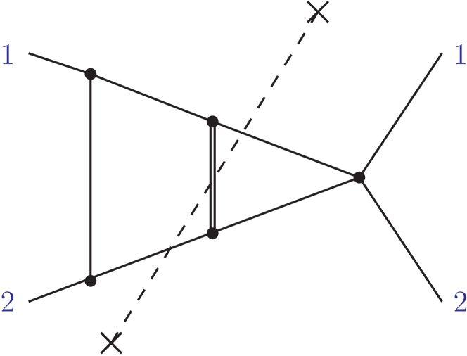
$\text{TTD}_{3}(1,1,1,1,1,1,1)$	$\text{TTE}_{3}(1,0,1,1,1,0,1)$	$\text{TTE}_{3}(1,1,1,1,1,1,0)$
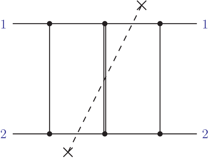
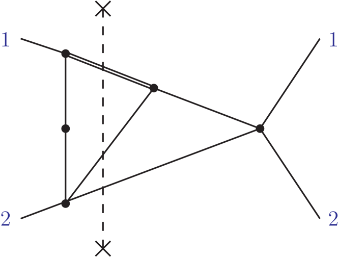
$\text{TTE}_{3}(1,1,1,1,1,1,1)$	$\text{TTF}_{3}(1,0,1,1,1,0,1)$	$\text{TTF}_{3}(1,0,1,1,1,0,2)$
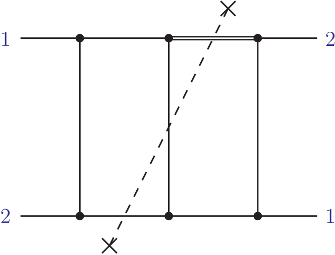
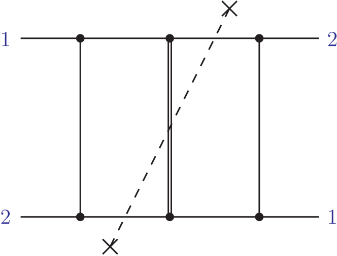
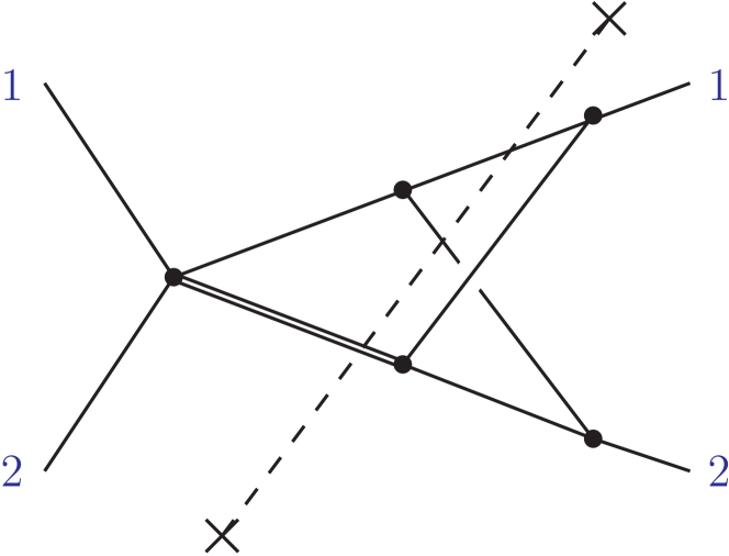
$\text{TTG}_{3}(1,1,1,1,1,1,1)$	$\text{TTH}_{3}(1,1,1,1,1,1,1)$	$\text{TTJ}_{3}(1,1,1,1,1,1,0)$
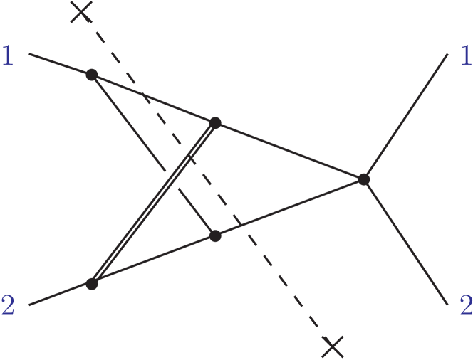
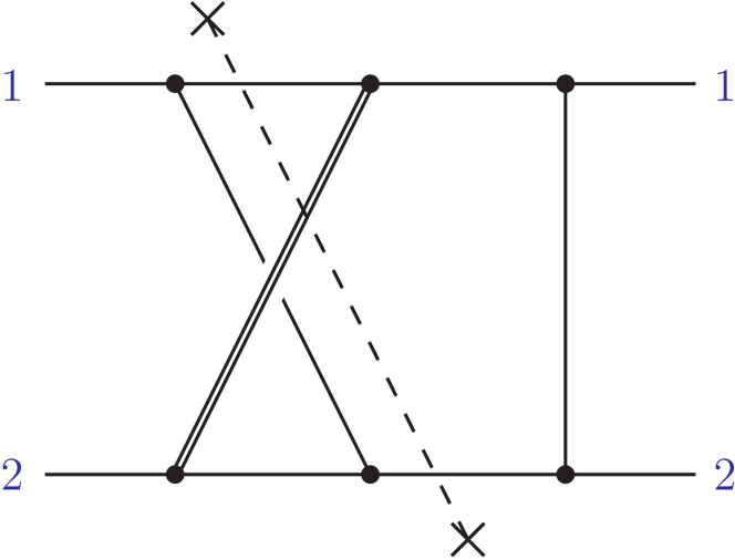
$\text{TTK}_{3}(1,1,1,1,1,1,0)$	$\text{TTK}_{3}(1,1,1,1,1,1,1)$

Figure 4: Three-particle cut diagrams appearing in our choice of canonical master integrals at NNLO.

Here we present a canonical basis we found at NNLO, together with the differential equation matrix $A$ it satisfies. All master integrals of topology $T$ in this basis have the form

$$M^{(T)}_{i}=\epsilon^{d_{i}}n_{i}(x)\sum_{k}c_{ik}T\left(\{a\}_{k}\right),$$ (55)

where $d_{i}$ is an integer, $n_{i}(x)$ is an $x$-dependent prefactor, $c_{ik}$ are numerical constants and $\{a\}_{k}$ are distinct sets of indices. All integrals are defined as single-cut integrals. The definitions of the individual topologies are given in fig. 2. Note that the choice of a canonical basis is not unique. In many cases we have found alternative master integrals forming a canonical basis which have a more complicated $n(\epsilon)$ normalization. We present here a basis of the simple monomial form in $\epsilon$ as eq. (55):

$$W_{1} =\epsilon\text{TTF}_{2}(2,0,2,1,0,1,0),$$

$$W_{2} =\epsilon^{3}(1-x)\text{TTF}_{2}(1,0,1,1,1,1,1),$$

$$W_{3} =\epsilon^{2}\text{TTF}_{2}(1,2,0,0,1,1,0),$$

$$W_{4} =\epsilon^{3}\text{TTF}_{2}(1,1,1,0,1,1,0),$$

$$W_{5} =\epsilon^{3}(1-x)\text{TTG}_{2}(1,1,1,1,1,1,1),$$

$$W_{6} =\epsilon^{3}(1-x)\text{TTJ}_{2}(1,1,1,1,1,1,0),$$ (56)

are the two-particle cut master integrals, whereas

$$V_{1} =\epsilon\text{TTA}_{3}(2,2,1,0,0,0,0),$$

$$V_{2} =\epsilon(1-x)\bigl{[}\text{TTA}_{3}(1,2,2,0,0,0,0)+2\text{TTA}_{3}(2,2,1,0,0,0,0)\bigr{]},$$

$$V_{3} =\epsilon^{3}\text{TTA}_{3}(1,1,1,1,0,1,0),$$

$$V_{4} =\epsilon^{3}(1-x)\text{TTA}_{3}(1,1,1,1,1,1,1),$$

$$V_{5} =\epsilon^{2}(1-x)\text{TTC}_{3}(1,2,1,0,1,1,0),$$

$$V_{6} =\epsilon^{3}(1-x)x\text{TTC}_{3}(1,1,1,1,1,1,1),$$

$$V_{7} =\epsilon^{3}(1-x)\text{TTD}_{3}(1,1,1,1,1,1,1),$$

$$V_{8} =\epsilon^{3}\text{TTE}_{3}(1,0,1,1,1,0,1),$$

$$V_{9} =\epsilon^{3}\text{TTE}_{3}(1,1,1,1,1,1,0),$$

$$V_{10} =\epsilon^{3}x\text{TTE}_{3}(1,1,1,1,1,1,1),$$

$$V_{11} =\epsilon^{3}\text{TTF}_{3}(1,0,1,1,1,0,1),$$

$$V_{12} =\epsilon^{2}x\text{TTF}_{3}(1,0,1,1,1,0,2),$$

$$V_{13} =\epsilon^{3}(1-x)\text{TTG}_{3}(1,1,1,1,1,1,1),$$

$$V_{14} =\epsilon^{3}(1+x)\text{TTH}_{3}(1,1,1,1,1,1,1),$$

$$V_{15} =\epsilon^{3}(1-x)\text{TTJ}_{3}(1,1,1,1,1,1,0),$$

$$V_{16} =\epsilon^{3}(1+x)\text{TTK}_{3}(1,1,1,1,1,1,0),$$

$$V_{17} =\epsilon^{3}x\bigl{[}\text{TTK}_{3}(1,1,1,1,1,1,1)-\text{TTK}_{3}(1,1,1,1,1,1,0)\bigr{]},$$ (57)

are the three-particle cut master integrals. They are normalized in such a way as to start at finite order. Two- and three-particle cut diagrams appearing in this basis are shown in figs. 3 and 4, respectively.

The two-particle cut master integrals satisfy the differential equations (4) and (7) with

$$a_{2}=\begin{pmatrix}0&0&0&0&0&0\\ 1&-1&0&0&0&0\\ 0&0&0&0&0&0\\ 1&-1&-2&-2&0&0\\ 2&-2&2&2&0&0\\ 0&0&-4&-4&0&0\\ \end{pmatrix},$$ (58)

$$b_{2}=\begin{pmatrix}2&0&0&0&0&0\\ 0&2&0&0&0&0\\ 0&0&3&0&0&0\\ 0&0&0&0&0&0\\ 0&0&6&0&2&0\\ 0&0&0&0&0&4\\ \end{pmatrix},$$ (59)

$$c_{2}=0,$$ (60)

whereas for the three-particle cut master integrals we have

$$a_{3}=\setcounter{MaxMatrixCols}{17}\begin{pmatrix}-3&1&0&0&0&0&0&0&0&0&0&0&0&0&0&0&0\\ -6&2&0&0&0&0&0&0&0&0&0&0&0&0&0&0&0\\ -1&\frac{1}{2}&-2&0&0&0&0&0&0&0&0&0&0&0&0&0&0\\ -2&1&-4&0&0&0&0&0&0&0&0&0&0&0&0&0&0\\ 0&-\frac{1}{2}&0&0&-1&0&0&0&0&0&0&0&0&0&0&0&0\\ -1&\frac{1}{2}&-2&0&0&-2&0&0&0&0&0&0&0&0&0&0&0\\ 0&1&0&0&2&0&0&0&0&0&0&0&0&0&0&0&0\\ -2&\frac{1}{2}&0&0&0&0&0&-2&0&0&0&0&0&0&0&0&0\\ 4&-1&0&0&0&0&0&1&-1&0&0&0&0&0&0&0&0\\ -5&\frac{3}{2}&0&0&0&0&0&-2&0&-2&0&0&0&0&0&0&0\\ -1&\frac{1}{4}&0&0&0&0&0&0&0&0&-1&1&0&0&0&0&0\\ -\frac{3}{2}&\frac{1}{2}&0&0&0&0&0&0&0&0&0&-2&0&0&0&0&0\\ -4&\frac{3}{2}&0&0&0&0&0&0&0&0&2&2&0&0&0&0&0\\ 2&0&0&0&0&0&0&2&-2&0&0&0&0&0&0&0&0\\ 1&-\frac{1}{2}&2&0&0&0&0&0&0&0&0&0&0&0&0&0&0\\ 3&-1&-2&0&0&0&0&0&0&0&-2&-2&0&0&0&0&0\\ 1&-\frac{1}{2}&2&0&0&0&0&0&0&0&0&0&0&0&0&0&-2\\ \end{pmatrix},$$ (61)

$$b_{3}=\setcounter{MaxMatrixCols}{17}\begin{pmatrix}0&1&0&0&0&0&0&0&0&0&0&0&0&0&0&0&0\\ 0&4&0&0&0&0&0&0&0&0&0&0&0&0&0&0&0\\ 0&0&0&0&0&0&0&0&0&0&0&0&0&0&0&0&0\\ 0&2&0&2&0&0&0&0&0&0&0&0&0&0&0&0&0\\ 0&-\frac{1}{2}&0&0&2&0&0&0&0&0&0&0&0&0&0&0&0\\ 0&0&0&0&-2&2&0&0&0&0&0&0&0&0&0&0&0\\ 0&1&0&0&2&0&2&0&0&0&0&0&0&0&0&0&0\\ 0&0&0&0&0&0&0&0&0&0&0&0&0&0&0&0&0\\ 0&0&0&0&0&0&0&0&0&0&0&0&0&0&0&0&0\\ 0&0&0&0&0&0&0&0&0&0&0&0&0&0&0&0&0\\ 0&0&0&0&0&0&0&0&0&0&0&0&0&0&0&0&0\\ -4&1&0&0&0&0&0&0&0&0&2&2&0&0&0&0&0\\ -4&\frac{3}{2}&0&0&0&0&0&0&0&0&2&2&2&0&0&0&0\\ 0&0&0&0&0&0&0&0&0&0&0&0&0&0&0&0&0\\ 0&0&0&0&0&0&0&0&0&0&0&0&0&0&4&0&0\\ 0&0&0&0&0&0&0&0&0&0&0&0&0&0&0&0&0\\ 4&-\frac{3}{2}&0&0&0&0&0&0&0&0&-2&-2&0&0&0&0&0\\ \end{pmatrix},$$ (62)

$$c_{3}=\setcounter{MaxMatrixCols}{17}\begin{pmatrix}0&0&0&0&0&0&0&0&0&0&0&0&0&0&0&0&0\\ 0&0&0&0&0&0&0&0&0&0&0&0&0&0&0&0&0\\ 0&0&0&0&0&0&0&0&0&0&0&0&0&0&0&0&0\\ 0&0&0&0&0&0&0&0&0&0&0&0&0&0&0&0&0\\ 0&0&0&0&0&0&0&0&0&0&0&0&0&0&0&0&0\\ 0&0&0&0&0&0&0&0&0&0&0&0&0&0&0&0&0\\ 0&0&0&0&0&0&0&0&0&0&0&0&0&0&0&0&0\\ 0&0&0&0&0&0&0&0&0&0&0&0&0&0&0&0&0\\ -4&1&0&0&0&0&0&-1&-1&0&0&0&0&0&0&0&0\\ 8&-2&0&0&0&0&0&2&2&0&0&0&0&0&0&0&0\\ 0&0&0&0&0&0&0&0&0&0&0&0&0&0&0&0&0\\ 0&0&0&0&0&0&0&0&0&0&0&0&0&0&0&0&0\\ 0&0&0&0&0&0&0&0&0&0&0&0&0&0&0&0&0\\ 0&0&0&0&0&0&0&0&0&0&0&0&0&-2&0&0&0\\ 0&0&0&0&0&0&0&0&0&0&0&0&0&0&0&0&0\\ 0&0&0&0&0&0&0&0&0&0&0&0&0&0&0&-4&0\\ 0&0&0&0&0&0&0&0&0&0&0&0&0&0&0&2&0\\ \end{pmatrix}.$$ (63)

As discussed previously, $(V_{1},V_{2})$ and $(V_{11},V_{12})$ form coupled differential equations. The other integrals form a triangular system, hence one can add a candidate integral to a subset of a canonical basis and check if it successfully gives a larger canonical basis or not, approaching a whole canonical basis step by step. Some of the integrals in the canonical basis given here are diagrammatically similar to those given in ref. Henn:2013pwa where four-point two-loop diagrams have been investigated as well, although with different kinematics.

We computed the given master integrals $W_{i}$ and $V_{i}$ up to order $\epsilon^{6}$ corresponding to a maximum weight of six in the appearing HPLs, using their reduction to the reduction basis and the $x\to 1$ limit of the latter as boundary conditions. We checked that the solutions for the master integrals in the canonical basis are pure functions. Furthermore, by applying the matrix $B^{-1}$ we transformed back to the reduction basis and found agreement with the results given in ref. Pak:2011hs up to the order in $\epsilon$ given there which is high enough for the N³LO calculation (see also the result in ref. Anastasiou:2012kq ). We emphasize that in the canonical basis master integrals decouple order by order in $\epsilon$ and therefore only the first term in the $x\to 1$ limit for each master integral is sufficient to fix all the boundary constants.

4 N³LO: example and solution

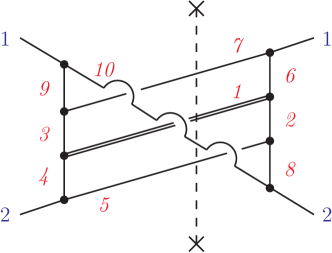
Figure 5: The sea snake topology $\text{TTS}_{4}(a_{1},a_{2},a_{3},a_{4},a_{5},a_{6},a_{7},a_{8},a_{9},a_{10},n_{11},n_{12})$. The notation is the same as in fig. 2. The indices $n_{11}$ and $n_{12}$ denote irreducible scalar products which appear in the numerator and are always less than or equal to zero.

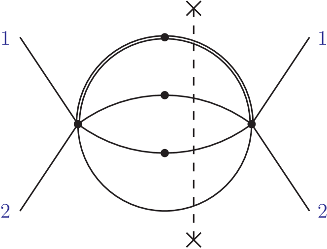
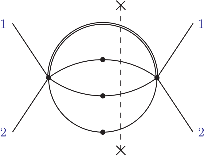
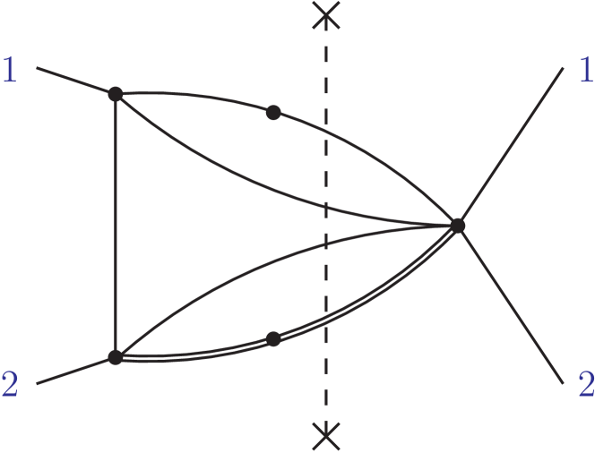
$\text{TTS}_{4}$ (2,0,0,0,2,0,2,0,0,1,0,0)	$\text{TTS}_{4}$ (1,0,0,0,2,0,2,0,0,2,0,0)	$\text{TTS}_{4}$ (2,0,1,0,1,0,2,0,0,1,0,0)
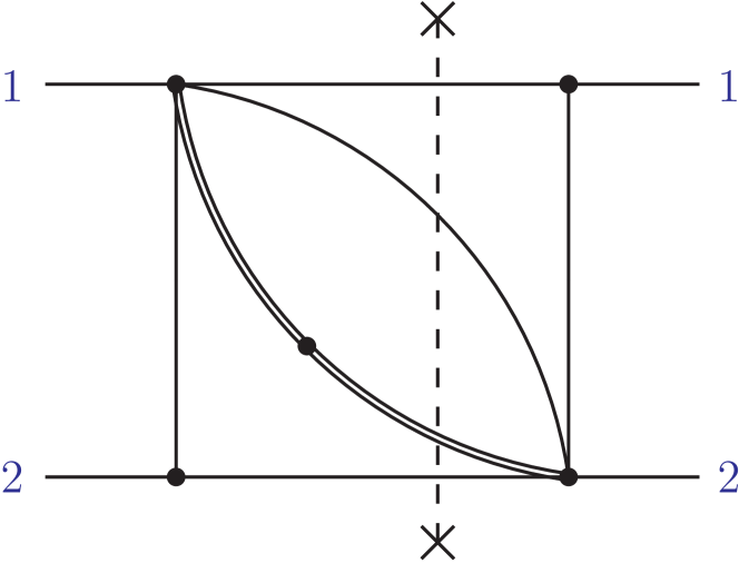
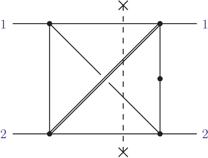
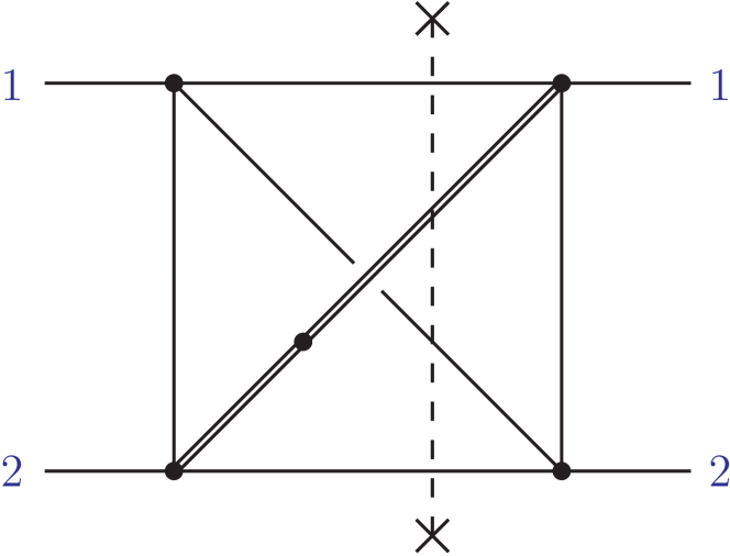
$\text{TTS}_{4}$ (2,0,0,1,1,1,1,0,0,1,0,0)	$\text{TTS}_{4}$ (1,2,1,0,1,0,1,0,0,1,0,0)	$\text{TTS}_{4}$ (2,1,1,0,1,0,1,0,0,1,0,0)
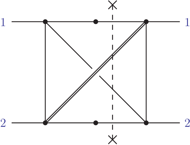
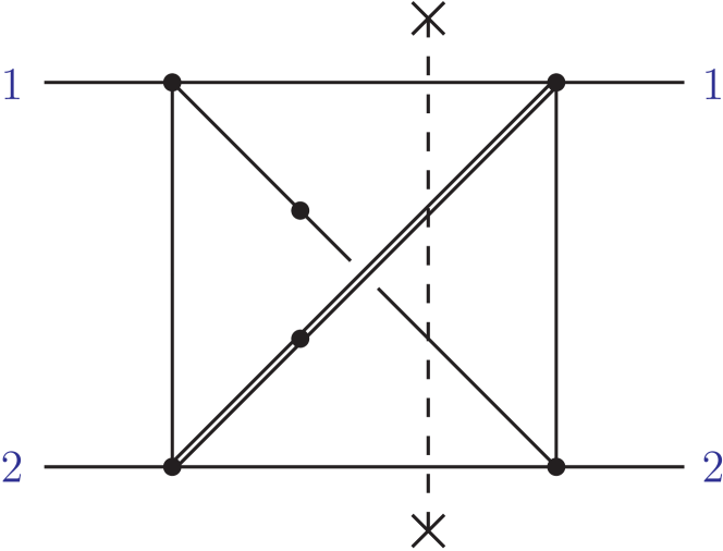
$\text{TTS}_{4}$ (1,1,1,0,2,0,2,0,0,1,0,0)	$\text{TTS}_{4}$ (1,2,2,0,1,0,1,0,0,1,0,0)	$\text{TTS}_{4}$ (2,1,1,0,1,0,1,0,0,2,0,0)
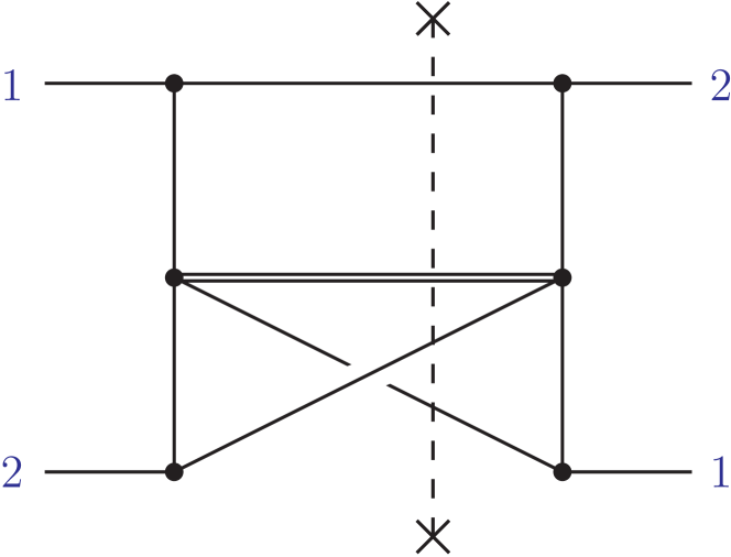
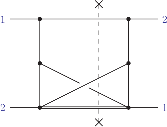
$\text{TTS}_{4}$ (1,0,0,1,1,1,1,1,1,1,0,0)	$\text{TTS}_{4}$ (1,1,1,0,1,0,1,1,1,1,0,0)

Figure 6: Diagrams appearing in our choice of canonical master integrals for the sea snake topology.

In this section we discuss the N³LO topology $\text{TTS}_{4}$, shown in fig. 5, which we refer to as sea snake topology. It is non-planar, has ten lines with two additional irreducible scalar products and exhibits a four-particle cut only. Integrals belonging to this topology are reduced to eleven master integrals, which we choose to be also of the form of eq. (55) and with the last two indices for the irreducible scalar products set to be zero, namely,

$$S_{1} =\epsilon^{2}\text{TTS}_{4}(2,0,0,0,2,0,2,0,0,1,0,0),$$

$$S_{2} =\epsilon^{2}(1-x)\left[\text{TTS}_{4}(1,0,0,0,2,0,2,0,0,2,0,0)+3\text{TTS}_{4}(2,0,0,0,2,0,2,0,0,1,0,0)\right],$$

$$S_{3} =\epsilon^{3}\text{TTS}_{4}(2,0,1,0,1,0,2,0,0,1,0,0),$$

$$S_{4} =\epsilon^{4}\text{TTS}_{4}(2,0,0,1,1,1,1,0,0,1,0,0),$$

$$S_{5} =\epsilon^{4}\text{TTS}_{4}(1,2,1,0,1,0,1,0,0,1,0,0),$$

$$S_{6} =\epsilon^{4}\text{TTS}_{4}(2,1,1,0,1,0,1,0,0,1,0,0),$$

$$S_{7} =\epsilon^{3}(1-x)\text{TTS}_{4}(1,1,1,0,2,0,2,0,0,1,0,0),$$

$$S_{8} =\epsilon^{3}x\text{TTS}_{4}(1,2,2,0,1,0,1,0,0,1,0,0),$$

$$S_{9} =\epsilon^{3}x\text{TTS}_{4}(2,1,1,0,1,0,1,0,0,2,0,0),$$

$$S_{10} =\epsilon^{5}\text{TTS}_{4}(1,0,0,1,1,1,1,1,1,1,0,0),$$

$$S_{11} =\epsilon^{5}\text{TTS}_{4}(1,1,1,0,1,0,1,1,1,1,0,0).$$ (64)

Diagrams appearing in this basis are shown in fig. 6.

The choice of master integrals $S_{1}$ and $S_{2}$ is motivated by the discussion given in section 3 in analogy to eq. (3.1). $S_{3}$ and $S_{4}$ are not coupled and can be found by trying possible candidates. $S_{10}$ and $S_{11}$ stem up to $\epsilon$-normalization from the reduction basis. This can be motivated from the sum of indices $a=8$ leading to the favored $e_{W}=1$ given in eq. (2.5), as discussed in section 2. Integrals $S_{5}$ to $S_{9}$ are coupled. It is worth mentioning that the subtopology spanned by their six propagators defines the $K_{4}$ topology discussed in ref. Henn:2013nsa . Although kinematics and mass-configuration are different from the present case, the basis integrals $S_{5}$ to $S_{9}$ can be established by direct diagrammatic correspondence to five of the seven coupled integrals for the off-shell $K_{4}$ case $g_{6}$, $\dots$, $g_{10}$ given in ref. Henn:2013nsa :

$$g_{6}\mathrel{\hat{=}}S_{6},\qquad g_{7}\mathrel{\hat{=}}S_{5},\qquad g_{8}\mathrel{\hat{=}}S_{7},\qquad g_{9}\mathrel{\hat{=}}S_{9},\qquad g_{10}\mathrel{\hat{=}}S_{8},$$ (65)

where “$\mathrel{\hat{=}}$” states that the indices of the integrals have the same structure. For this case of five coupled master integrals, we do not use the algorithm described in section 3.2.5, because the equations to be solved become highly complicated.

The basis given here satisfies the differential equation of eq. (4) with eq. (7):

$$a_{4}=\setcounter{MaxMatrixCols}{11}\begin{pmatrix}-4&1&0&0&0&0&0&0&0&0&0\\ -12&3&0&0&0&0&0&0&0&0&0\\ -\frac{1}{2}&0&-2&0&0&0&0&0&0&0&0\\ 1&-\frac{1}{6}&0&-3&0&0&0&0&0&0&0\\ -\frac{1}{6}&0&0&0&-\frac{2}{3}&\frac{2}{3}&-\frac{1}{6}&\frac{1}{2}&\frac{1}{3}&0&0\\ \frac{5}{6}&0&1&0&\frac{7}{3}&-\frac{7}{3}&\frac{7}{12}&\frac{1}{4}&-\frac{1}{6}&0&0\\ \frac{11}{3}&-\frac{1}{2}&2&0&\frac{14}{3}&-\frac{14}{3}&\frac{7}{6}&\frac{5}{2}&\frac{8}{3}&0&0\\ \frac{7}{3}&-\frac{1}{2}&2&0&-\frac{2}{3}&\frac{2}{3}&-\frac{1}{6}&-\frac{7}{2}&-\frac{2}{3}&0&0\\ \frac{7}{3}&-\frac{1}{2}&2&0&-\frac{2}{3}&\frac{2}{3}&-\frac{1}{6}&-\frac{1}{2}&-\frac{11}{3}&0&0\\ 0&-\frac{1}{6}&0&2&0&0&0&0&0&-3&0\\ -3&0&-7&0&-13&-2&-\frac{3}{2}&-\frac{5}{2}&-2&0&-3\\ \end{pmatrix},$$ (66)

$$b_{4}=\setcounter{MaxMatrixCols}{11}\begin{pmatrix}0&1&0&0&0&0&0&0&0&0&0\\ 0&6&0&0&0&0&0&0&0&0&0\\ 0&0&0&0&0&0&0&0&0&0&0\\ 0&0&0&0&0&0&0&0&0&0&0\\ 0&0&0&0&0&0&0&0&0&0&0\\ 0&0&0&0&0&0&0&0&0&0&0\\ \frac{11}{3}&-\frac{1}{2}&6&0&\frac{50}{3}&\frac{10}{3}&\frac{37}{6}&\frac{7}{2}&\frac{5}{3}&0&0\\ \frac{11}{3}&-\frac{1}{2}&6&0&\frac{50}{3}&\frac{10}{3}&\frac{1}{6}&\frac{7}{2}&\frac{5}{3}&0&0\\ -\frac{11}{3}&-\frac{1}{2}&-6&0&-\frac{50}{3}&-\frac{10}{3}&-\frac{19}{6}&-\frac{7}{2}&-\frac{5}{3}&0&0\\ 0&0&0&0&0&0&0&0&0&0&0\\ 0&0&0&0&0&0&0&0&0&0&0\\ \end{pmatrix}$$ (67)

and

$$c_{4}=0.$$ (68)

We computed the master integrals $S_{i}$ up to order $\epsilon^{6}$ corresponding to a maximum weight of six in the HPLs. As boundary conditions we computed the master integrals in the reduction basis in the $x\to 1$ limit with our Mathematica implementation of the soft expansion algorithm given in ref. Anastasiou:2013srw , using the program FIRE for reduction. It is worth mentioning that all master integrals are reduced to the four-particle phase space integral only, i.e., the integral $F_{1}(\epsilon)$ given in ref. Anastasiou:2013srw which is known for general values of $\epsilon$, therefore the result given here can be extended to arbitrary orders in $\epsilon$. We checked our results transformed to the reduction basis against the soft expansion around $x=1$, including at least three non-vanishing terms in the expansion. Furthermore, we found that all $S_{i}$ are indeed pure functions. The results, up to order $\epsilon^{5}$ for brevity, are given in appendix A.

5 Conclusions and outlook

In this work we recomputed all necessary double-real and real-virtual master integrals for $gg\to h$ at NNLO within the framework of canonical differential equations Henn:2013pwa . By solving a non-planar three-loop topology as well, we have explicitly shown the use of the method to Higgs production in gluon fusion in full $x$-dependence at N³LO. The method can be applied to other master integrals at N³LO, which will contribute to the completion of the calculation of the total inclusive Higgs production cross section with full $x$-dependence in the future. To accomplish this, one needs to provide boundary conditions for the differential equations. For the triple-real emission diagrams, the reduction of phase space integrals in the soft limit Anastasiou:2013srw works efficiently to obtain the soft expansions around threshold. For other diagrams containing loop integrals, techniques such as asymptotic expansions by strategy of regions Beneke:1997zp ; Smirnov:2002pj ; Anastasiou:2013mca , those in the $\alpha$-parameter representations Smirnov:1999bza ; Smirnov:2012gma or asymptotic expansions of Mellin-Barnes integral representations Smirnov:2012gma may be useful to obtain the soft expansions. Sophisticated treatments for phase space integrals may also do the job. In any case, the fact that the framework of canonical differential equations requires only the leading terms of expansions for boundary conditions can make the computation simple.

Furthermore, working in this new framework we were able to derive a new criterion to find a canonical master integral being part of a coupled system by use of a characteristic form for higher order differential equations, allowing also for the construction of a canonical basis for the coupled integrals. This criterion was derived in a quite general way and can also be used in coupled systems of differential equations for master integrals appearing in other processes.

Appendix A Results for sea snake topology

In the appendix, we present the results of the master integrals $S_{i}$ for the sea snake topology $\text{TTS}_{4}$. We have normalized the results by multiplying an $\epsilon$-dependent prefactor, which is chosen such that the four-particle phase space integral in the limit $x\to 1$, corresponding to $F_{1}(\epsilon)$ defined in ref. Anastasiou:2013srw , becomes

$$\lim_{x\to 1}\text{TTS}_{4}(1,0,0,0,1,0,1,0,0,1,0,0)=\frac{\Gamma^{3}(1-\epsilon)}{\Gamma(6-6\epsilon)\Gamma^{3}(1+\epsilon)}.$$ (69)

Furthermore, we omit the common argument $x$ of HPLs as $\operatorname{H}_{i_{1},\dots i_{n}}:=\operatorname{H}_{i_{1},\dots i_{n}}(x)$.

$$S_{1} =1+2\epsilon\big{[}\operatorname{H}_{0}+3\operatorname{H}_{1}\big{]}+2\epsilon^{2}\big{[}6\operatorname{H}_{2}-\operatorname{H}_{0,0}+3\operatorname{H}_{1,0}+18\operatorname{H}_{1,1}-12\zeta_{2}\big{]}-2\epsilon^{3}\big{[}6\operatorname{H}_{3}-18\operatorname{H}_{1,2}$$

$$-6\operatorname{H}_{2,0}-36\operatorname{H}_{2,1}-\operatorname{H}_{0,0,0}+3\operatorname{H}_{1,0,0}-18\operatorname{H}_{1,1,0}-108\operatorname{H}_{1,1,1}+\big{(}6\operatorname{H}_{0}+54\operatorname{H}_{1}\big{)}\zeta_{2}+32\zeta_{3}\big{]}$$

$$+2\epsilon^{4}\big{[}6\operatorname{H}_{4}-18\operatorname{H}_{1,3}+36\operatorname{H}_{2,2}-6\operatorname{H}_{3,0}-36\operatorname{H}_{3,1}+108\operatorname{H}_{1,1,2}+18\operatorname{H}_{1,2,0}+108\operatorname{H}_{1,2,1}$$

$$-6\operatorname{H}_{2,0,0}+36\operatorname{H}_{2,1,0}+216\operatorname{H}_{2,1,1}-\operatorname{H}_{0,0,0,0}+3\operatorname{H}_{1,0,0,0}-18\operatorname{H}_{1,1,0,0}+108\operatorname{H}_{1,1,1,0}$$

$$+648\operatorname{H}_{1,1,1,1}+\big{(}-108\operatorname{H}_{2}+6\operatorname{H}_{0,0}-18\operatorname{H}_{1,0}-324\operatorname{H}_{1,1}\big{)}\zeta_{2}+123\zeta_{4}+\big{(}-10\operatorname{H}_{0}$$

$$-138\operatorname{H}_{1}\big{)}\zeta_{3}\big{]}-2\epsilon^{5}\big{[}6\operatorname{H}_{5}-18\operatorname{H}_{1,4}+36\operatorname{H}_{2,3}+36\operatorname{H}_{3,2}-6\operatorname{H}_{4,0}-36\operatorname{H}_{4,1}+108\operatorname{H}_{1,1,3}$$

$$-108\operatorname{H}_{1,2,2}+18\operatorname{H}_{1,3,0}+108\operatorname{H}_{1,3,1}-216\operatorname{H}_{2,1,2}-36\operatorname{H}_{2,2,0}-216\operatorname{H}_{2,2,1}-6\operatorname{H}_{3,0,0}$$

$$+36\operatorname{H}_{3,1,0}+216\operatorname{H}_{3,1,1}-648\operatorname{H}_{1,1,1,2}-108\operatorname{H}_{1,1,2,0}-648\operatorname{H}_{1,1,2,1}+18\operatorname{H}_{1,2,0,0}$$

$$-108\operatorname{H}_{1,2,1,0}-648\operatorname{H}_{1,2,1,1}-6\operatorname{H}_{2,0,0,0}+36\operatorname{H}_{2,1,0,0}-216\operatorname{H}_{2,1,1,0}-1296\operatorname{H}_{2,1,1,1}$$

$$-\operatorname{H}_{0,0,0,0,0}+3\operatorname{H}_{1,0,0,0,0}-18\operatorname{H}_{1,1,0,0,0}+108\operatorname{H}_{1,1,1,0,0}-648\operatorname{H}_{1,1,1,1,0}-3888\operatorname{H}_{1,1,1,1,1}$$

$$+\big{(}-21\operatorname{H}_{0}-513\operatorname{H}_{1}\big{)}\zeta_{4}+\zeta_{2}\big{(}-108\operatorname{H}_{3}+324\operatorname{H}_{1,2}+36\operatorname{H}_{2,0}+648\operatorname{H}_{2,1}+6\operatorname{H}_{0,0,0}$$

$$-18\operatorname{H}_{1,0,0}+108\operatorname{H}_{1,1,0}+1944\operatorname{H}_{1,1,1}-444\zeta_{3}\big{)}+\big{(}276\operatorname{H}_{2}-10\operatorname{H}_{0,0}+30\operatorname{H}_{1,0}$$

$$+828\operatorname{H}_{1,1}\big{)}\zeta_{3}+324\zeta_{5}\big{]}+\mathcal{O}\big{(}\epsilon^{6}\big{)},$$ (70)

$$S_{2} =6+6\epsilon\big{[}\operatorname{H}_{0}+6\operatorname{H}_{1}\big{]}+6\epsilon^{2}\big{[}6\operatorname{H}_{2}-\operatorname{H}_{0,0}+6\operatorname{H}_{1,0}+36\operatorname{H}_{1,1}-18\zeta_{2}\big{]}-6\epsilon^{3}\big{[}6\operatorname{H}_{3}-36\operatorname{H}_{1,2}$$

$$-6\operatorname{H}_{2,0}-36\operatorname{H}_{2,1}-\operatorname{H}_{0,0,0}+6\operatorname{H}_{1,0,0}-36\operatorname{H}_{1,1,0}-216\operatorname{H}_{1,1,1}+\big{(}6\operatorname{H}_{0}+108\operatorname{H}_{1}\big{)}\zeta_{2}$$

$$+46\zeta_{3}\big{]}+6\epsilon^{4}\big{[}6\operatorname{H}_{4}-36\operatorname{H}_{1,3}+36\operatorname{H}_{2,2}-6\operatorname{H}_{3,0}-36\operatorname{H}_{3,1}+216\operatorname{H}_{1,1,2}+36\operatorname{H}_{1,2,0}$$

$$+216\operatorname{H}_{1,2,1}-6\operatorname{H}_{2,0,0}+36\operatorname{H}_{2,1,0}+216\operatorname{H}_{2,1,1}-\operatorname{H}_{0,0,0,0}+6\operatorname{H}_{1,0,0,0}-36\operatorname{H}_{1,1,0,0}$$

$$+216\operatorname{H}_{1,1,1,0}+1296\operatorname{H}_{1,1,1,1}+\big{(}-108\operatorname{H}_{2}+6\operatorname{H}_{0,0}-36\operatorname{H}_{1,0}-648\operatorname{H}_{1,1}\big{)}\zeta_{2}+171\zeta_{4}$$

$$+\big{(}-10\operatorname{H}_{0}-276\operatorname{H}_{1}\big{)}\zeta_{3}\big{]}-6\epsilon^{5}\big{[}6\operatorname{H}_{5}-36\operatorname{H}_{1,4}+36\operatorname{H}_{2,3}+36\operatorname{H}_{3,2}-6\operatorname{H}_{4,0}-36\operatorname{H}_{4,1}$$

$$+216\operatorname{H}_{1,1,3}-216\operatorname{H}_{1,2,2}+36\operatorname{H}_{1,3,0}+216\operatorname{H}_{1,3,1}-216\operatorname{H}_{2,1,2}-36\operatorname{H}_{2,2,0}-216\operatorname{H}_{2,2,1}$$

$$-6\operatorname{H}_{3,0,0}+36\operatorname{H}_{3,1,0}+216\operatorname{H}_{3,1,1}-1296\operatorname{H}_{1,1,1,2}-216\operatorname{H}_{1,1,2,0}-1296\operatorname{H}_{1,1,2,1}$$

$$+36\operatorname{H}_{1,2,0,0}-216\operatorname{H}_{1,2,1,0}-1296\operatorname{H}_{1,2,1,1}-6\operatorname{H}_{2,0,0,0}+36\operatorname{H}_{2,1,0,0}-216\operatorname{H}_{2,1,1,0}$$

$$-1296\operatorname{H}_{2,1,1,1}-\operatorname{H}_{0,0,0,0,0}+6\operatorname{H}_{1,0,0,0,0}-36\operatorname{H}_{1,1,0,0,0}+216\operatorname{H}_{1,1,1,0,0}-1296\operatorname{H}_{1,1,1,1,0}$$

$$-7776\operatorname{H}_{1,1,1,1,1}+\big{(}-21\operatorname{H}_{0}-1026\operatorname{H}_{1}\big{)}\zeta_{4}+\zeta_{2}\big{(}-108\operatorname{H}_{3}+648\operatorname{H}_{1,2}+36\operatorname{H}_{2,0}+648\operatorname{H}_{2,1}$$

$$+6\operatorname{H}_{0,0,0}-36\operatorname{H}_{1,0,0}+216\operatorname{H}_{1,1,0}+3888\operatorname{H}_{1,1,1}-612\zeta_{3}\big{)}+\big{(}276\operatorname{H}_{2}-10\operatorname{H}_{0,0}+60\operatorname{H}_{1,0}$$

$$+1656\operatorname{H}_{1,1}\big{)}\zeta_{3}+450\zeta_{5}\big{]}+\mathcal{O}\big{(}\epsilon^{6}\big{)},$$ (71)

$$S_{3} =-\frac{\epsilon}{2}\operatorname{H}_{0}-3\epsilon^{2}\big{[}\operatorname{H}_{2}-\zeta_{2}\big{]}+\epsilon^{3}\big{[}-3\operatorname{H}_{2,0}-18\operatorname{H}_{2,1}+\operatorname{H}_{0,0,0}+6\operatorname{H}_{0}\zeta_{2}+12\zeta_{3}\big{]}$$

$$+\epsilon^{4}\big{[}6\operatorname{H}_{4}-18\operatorname{H}_{2,2}+3\operatorname{H}_{2,0,0}-18\operatorname{H}_{2,1,0}-108\operatorname{H}_{2,1,1}-3\operatorname{H}_{0,0,0,0}+\big{(}54\operatorname{H}_{2}-6\operatorname{H}_{0,0}\big{)}\zeta_{2}$$

$$-51\zeta_{4}+8\operatorname{H}_{0}\zeta_{3}\big{]}+\epsilon^{5}\big{[}-18\operatorname{H}_{5}+18\operatorname{H}_{2,3}+6\operatorname{H}_{4,0}+36\operatorname{H}_{4,1}-108\operatorname{H}_{2,1,2}-18\operatorname{H}_{2,2,0}$$

$$-108\operatorname{H}_{2,2,1}-3\operatorname{H}_{2,0,0,0}+18\operatorname{H}_{2,1,0,0}-108\operatorname{H}_{2,1,1,0}-648\operatorname{H}_{2,1,1,1}+7\operatorname{H}_{0,0,0,0,0}-21\operatorname{H}_{0}\zeta_{4}$$

$$+\zeta_{2}\big{(}18\operatorname{H}_{2,0}+324\operatorname{H}_{2,1}+6\operatorname{H}_{0,0,0}-192\zeta_{3}\big{)}+\big{(}138\operatorname{H}_{2}-6\operatorname{H}_{0,0}\big{)}\zeta_{3}+138\zeta_{5}\big{]}+\mathcal{O}\big{(}\epsilon^{6}\big{)},$$ (72)

$$S_{4} =\epsilon^{2}\operatorname{H}_{0,0}+2\epsilon^{3}\big{[}3\operatorname{H}_{3}-2\operatorname{H}_{0,0,0}-3\operatorname{H}_{0}\zeta_{2}-3\zeta_{3}\big{]}+\epsilon^{4}\big{[}-24\operatorname{H}_{4}+6\operatorname{H}_{3,0}+36\operatorname{H}_{3,1}$$

$$+13\operatorname{H}_{0,0,0,0}+12\operatorname{H}_{0,0}\zeta_{2}+33\zeta_{4}\big{]}+2\epsilon^{5}\big{[}39\operatorname{H}_{5}+18\operatorname{H}_{3,2}-12\operatorname{H}_{4,0}-72\operatorname{H}_{4,1}-3\operatorname{H}_{3,0,0}$$

$$+18\operatorname{H}_{3,1,0}+108\operatorname{H}_{3,1,1}-20\operatorname{H}_{0,0,0,0,0}-12\operatorname{H}_{0}\zeta_{4}-5\operatorname{H}_{0,0}\zeta_{3}+\zeta_{2}\big{(}-54\operatorname{H}_{3}-15\operatorname{H}_{0,0,0}$$

$$+36\zeta_{3}\big{)}-33\zeta_{5}\big{]}+\mathcal{O}\big{(}\epsilon^{6}\big{)},$$ (73)

$$S_{5} =\frac{\epsilon^{3}}{2}\big{[}\operatorname{H}_{2,0}+\operatorname{H}_{0,0,0}+\operatorname{H}_{0}\zeta_{2}+2\zeta_{3}\big{]}+\epsilon^{4}\big{[}3\operatorname{H}_{4}+3\operatorname{H}_{2,2}-2\operatorname{H}_{3,0}-\operatorname{H}_{2,0,0}+\operatorname{H}_{2,1,0}$$

$$-4\operatorname{H}_{0,0,0,0}+\big{(}-2\operatorname{H}_{2}-5\operatorname{H}_{0,0}\big{)}\zeta_{2}-2\zeta_{4}-\operatorname{H}_{0}\zeta_{3}\big{]}+\frac{\epsilon^{5}}{8}\big{[}-192\operatorname{H}_{5}-48\operatorname{H}_{2,3}-96\operatorname{H}_{3,2}$$

$$+84\operatorname{H}_{4,0}+144\operatorname{H}_{4,1}+48\operatorname{H}_{2,1,2}+4\operatorname{H}_{2,2,0}+144\operatorname{H}_{2,2,1}+32\operatorname{H}_{3,0,0}-32\operatorname{H}_{3,1,0}$$

$$-20\operatorname{H}_{2,0,0,0}-48\operatorname{H}_{2,1,0,0}+172\operatorname{H}_{0,0,0,0,0}+323\operatorname{H}_{0}\zeta_{4}+\zeta_{2}\big{(}64\operatorname{H}_{3}-20\operatorname{H}_{2,0}-48\operatorname{H}_{2,1}$$

$$+204\operatorname{H}_{0,0,0}-56\zeta_{3}\big{)}+\big{(}56\operatorname{H}_{2}+24\operatorname{H}_{0,0}\big{)}\zeta_{3}+184\zeta_{5}\big{]}+\mathcal{O}\big{(}\epsilon^{6}\big{)},$$ (74)

$$S_{6} =\frac{\epsilon^{4}}{4}\big{[}4\operatorname{H}_{3,0}+8\operatorname{H}_{2,0,0}+4\operatorname{H}_{2,1,0}+8\operatorname{H}_{0,0,0,0}+\big{(}4\operatorname{H}_{2}+4\operatorname{H}_{0,0}\big{)}\zeta_{2}-17\zeta_{4}-4\operatorname{H}_{0}\zeta_{3}\big{]}$$

$$+\frac{\epsilon^{5}}{2}\big{[}24\operatorname{H}_{5}+24\operatorname{H}_{2,3}+12\operatorname{H}_{3,2}-12\operatorname{H}_{4,0}+12\operatorname{H}_{2,1,2}+6\operatorname{H}_{2,2,0}-16\operatorname{H}_{3,0,0}-2\operatorname{H}_{3,1,0}$$

$$+20\operatorname{H}_{2,1,0,0}+16\operatorname{H}_{2,1,1,0}-36\operatorname{H}_{0,0,0,0,0}-29\operatorname{H}_{0}\zeta_{4}+\big{(}-24\operatorname{H}_{2}-6\operatorname{H}_{0,0}\big{)}\zeta_{3}+\zeta_{2}\big{(}-14\operatorname{H}_{3}$$

$$-18\operatorname{H}_{2,0}+4\operatorname{H}_{2,1}-36\operatorname{H}_{0,0,0}+10\zeta_{3}\big{)}-27\zeta_{5}\big{]}+\mathcal{O}\big{(}\epsilon^{6}\big{)},$$ (75)

$$S_{7} =-\frac{3}{2}+\frac{\epsilon}{4}\big{[}-7\operatorname{H}_{0}-36\operatorname{H}_{1}\big{]}+\frac{\epsilon^{2}}{2}\big{[}-21\operatorname{H}_{2}+4\operatorname{H}_{0,0}-19\operatorname{H}_{1,0}-108\operatorname{H}_{1,1}+56\zeta_{2}\big{]}$$

$$+\frac{\epsilon^{3}}{4}\big{[}48\operatorname{H}_{3}-228\operatorname{H}_{1,2}-37\operatorname{H}_{2,0}-252\operatorname{H}_{2,1}-\operatorname{H}_{0,0,0}+48\operatorname{H}_{1,0,0}-216\operatorname{H}_{1,1,0}-1296\operatorname{H}_{1,1,1}$$

$$+\big{(}41\operatorname{H}_{0}+660\operatorname{H}_{1}\big{)}\zeta_{2}+262\zeta_{3}\big{]}+\frac{\epsilon^{4}}{8}\big{[}-12\operatorname{H}_{4}+576\operatorname{H}_{1,3}-444\operatorname{H}_{2,2}+72\operatorname{H}_{3,0}$$

$$+576\operatorname{H}_{3,1}-2592\operatorname{H}_{1,1,2}-412\operatorname{H}_{1,2,0}-2736\operatorname{H}_{1,2,1}+80\operatorname{H}_{2,0,0}-476\operatorname{H}_{2,1,0}-3024\operatorname{H}_{2,1,1}$$

$$-68\operatorname{H}_{0,0,0,0}-52\operatorname{H}_{1,0,0,0}+560\operatorname{H}_{1,1,0,0}-2528\operatorname{H}_{1,1,1,0}-15552\operatorname{H}_{1,1,1,1}+\big{(}1480\operatorname{H}_{2}$$

$$-204\operatorname{H}_{0,0}+380\operatorname{H}_{1,0}+7840\operatorname{H}_{1,1}\big{)}\zeta_{2}-2547\zeta_{4}+\big{(}68\operatorname{H}_{0}+3160\operatorname{H}_{1}\big{)}\zeta_{3}\big{]}+\frac{\epsilon^{5}}{16}\big{[}-816\operatorname{H}_{5}$$

$$-624\operatorname{H}_{1,4}+960\operatorname{H}_{2,3}+864\operatorname{H}_{3,2}+84\operatorname{H}_{4,0}-144\operatorname{H}_{4,1}+6720\operatorname{H}_{1,1,3}-4944\operatorname{H}_{1,2,2}$$

$$+944\operatorname{H}_{1,3,0}+6912\operatorname{H}_{1,3,1}-5712\operatorname{H}_{2,1,2}-940\operatorname{H}_{2,2,0}-5328\operatorname{H}_{2,2,1}-192\operatorname{H}_{3,0,0}$$

$$+1008\operatorname{H}_{3,1,0}+6912\operatorname{H}_{3,1,1}-30336\operatorname{H}_{1,1,1,2}-4800\operatorname{H}_{1,1,2,0}-31104\operatorname{H}_{1,1,2,1}+864\operatorname{H}_{1,2,0,0}$$

$$-5232\operatorname{H}_{1,2,1,0}-32832\operatorname{H}_{1,2,1,1}-268\operatorname{H}_{2,0,0,0}+928\operatorname{H}_{2,1,0,0}-5920\operatorname{H}_{2,1,1,0}-36288\operatorname{H}_{2,1,1,1}$$

$$+596\operatorname{H}_{0,0,0,0,0}-464\operatorname{H}_{1,0,0,0,0}-864\operatorname{H}_{1,1,0,0,0}+6464\operatorname{H}_{1,1,1,0,0}-30080\operatorname{H}_{1,1,1,1,0}$$

$$-186624\operatorname{H}_{1,1,1,1,1}+\big{(}1343\operatorname{H}_{0}-27600\operatorname{H}_{1}\big{)}\zeta_{4}+\zeta_{2}\big{(}-3312\operatorname{H}_{3}+16128\operatorname{H}_{1,2}+764\operatorname{H}_{2,0}$$

$$+17936\operatorname{H}_{2,1}+972\operatorname{H}_{0,0,0}-1888\operatorname{H}_{1,0,0}+4032\operatorname{H}_{1,1,0}+93568\operatorname{H}_{1,1,1}-13352\zeta_{3}\big{)}$$

$$+\big{(}7816\operatorname{H}_{2}-200\operatorname{H}_{0,0}+720\operatorname{H}_{1,0}+38208\operatorname{H}_{1,1}\big{)}\zeta_{3}+8976\zeta_{5}\big{]}+\mathcal{O}\big{(}\epsilon^{6}\big{)},$$ (76)

$$S_{8} =-\frac{\epsilon}{4}\operatorname{H}_{0}+\frac{\epsilon^{2}}{2}\big{[}-3\operatorname{H}_{2}+3\operatorname{H}_{0,0}+2\operatorname{H}_{1,0}+5\zeta_{2}\big{]}+\frac{\epsilon^{3}}{4}\big{[}36\operatorname{H}_{3}+24\operatorname{H}_{1,2}-19\operatorname{H}_{2,0}$$

$$-36\operatorname{H}_{2,1}-27\operatorname{H}_{0,0,0}+12\operatorname{H}_{1,1,0}+\big{(}-37\operatorname{H}_{0}-12\operatorname{H}_{1}\big{)}\zeta_{2}-2\zeta_{3}\big{]}+\frac{\epsilon^{4}}{4}\big{[}-162\operatorname{H}_{4}$$

$$-114\operatorname{H}_{2,2}+78\operatorname{H}_{3,0}+216\operatorname{H}_{3,1}+72\operatorname{H}_{1,1,2}+16\operatorname{H}_{1,2,0}+144\operatorname{H}_{1,2,1}+8\operatorname{H}_{2,0,0}-74\operatorname{H}_{2,1,0}$$

$$-216\operatorname{H}_{2,1,1}+108\operatorname{H}_{0,0,0,0}-20\operatorname{H}_{1,0,0,0}-8\operatorname{H}_{1,1,0,0}+32\operatorname{H}_{1,1,1,0}+\big{(}148\operatorname{H}_{2}+132\operatorname{H}_{0,0}$$

$$-56\operatorname{H}_{1,0}-40\operatorname{H}_{1,1}\big{)}\zeta_{2}+215\zeta_{4}+\big{(}10\operatorname{H}_{0}+8\operatorname{H}_{1}\big{)}\zeta_{3}\big{]}+\frac{\epsilon^{5}}{16}\big{[}2592\operatorname{H}_{5}-480\operatorname{H}_{1,4}$$

$$+192\operatorname{H}_{2,3}+1872\operatorname{H}_{3,2}-1188\operatorname{H}_{4,0}-3888\operatorname{H}_{4,1}-192\operatorname{H}_{1,1,3}+384\operatorname{H}_{1,2,2}+80\operatorname{H}_{1,3,0}$$

$$-1776\operatorname{H}_{2,1,2}-340\operatorname{H}_{2,2,0}-2736\operatorname{H}_{2,2,1}-192\operatorname{H}_{3,0,0}+1344\operatorname{H}_{3,1,0}+5184\operatorname{H}_{3,1,1}$$

$$+768\operatorname{H}_{1,1,1,2}+144\operatorname{H}_{1,1,2,0}+1728\operatorname{H}_{1,1,2,1}-96\operatorname{H}_{1,2,0,0}+480\operatorname{H}_{1,2,1,0}+3456\operatorname{H}_{1,2,1,1}$$

$$+236\operatorname{H}_{2,0,0,0}+288\operatorname{H}_{2,1,0,0}-1248\operatorname{H}_{2,1,1,0}-5184\operatorname{H}_{2,1,1,1}-1620\operatorname{H}_{0,0,0,0,0}+352\operatorname{H}_{1,0,0,0,0}$$

$$-240\operatorname{H}_{1,1,0,0,0}-256\operatorname{H}_{1,1,1,0,0}+256\operatorname{H}_{1,1,1,1,0}+\big{(}-2935\operatorname{H}_{0}+2964\operatorname{H}_{1}\big{)}\zeta_{4}+\zeta_{2}\big{(}-3120\operatorname{H}_{3}$$

$$-1632\operatorname{H}_{1,2}+836\operatorname{H}_{2,0}+3120\operatorname{H}_{2,1}-1836\operatorname{H}_{0,0,0}+560\operatorname{H}_{1,0,0}-528\operatorname{H}_{1,1,0}-512\operatorname{H}_{1,1,1}$$

$$-264\zeta_{3}\big{)}+\big{(}952\operatorname{H}_{2}-168\operatorname{H}_{0,0}-96\operatorname{H}_{1,0}+288\operatorname{H}_{1,1}\big{)}\zeta_{3}-176\zeta_{5}\big{]}+\mathcal{O}\big{(}\epsilon^{6}\big{)},$$ (77)

$$S_{9} =-\frac{1}{4}+\frac{\epsilon}{2}\big{[}\operatorname{H}_{0}-3\operatorname{H}_{1}\big{]}+\frac{\epsilon^{2}}{4}\big{[}12\operatorname{H}_{2}-3\operatorname{H}_{0,0}-7\operatorname{H}_{1,0}-36\operatorname{H}_{1,1}-\zeta_{2}\big{]}+\frac{\epsilon^{3}}{2}\big{[}-9\operatorname{H}_{3}$$

$$-21\operatorname{H}_{1,2}+7\operatorname{H}_{2,0}+36\operatorname{H}_{2,1}-21\operatorname{H}_{1,1,0}-108\operatorname{H}_{1,1,1}+\big{(}-2\operatorname{H}_{0}+54\operatorname{H}_{1}\big{)}\zeta_{2}+\zeta_{3}\big{]}$$

$$+\frac{\epsilon^{4}}{16}\big{[}336\operatorname{H}_{2,2}-84\operatorname{H}_{3,0}-432\operatorname{H}_{3,1}-1008\operatorname{H}_{1,1,2}-196\operatorname{H}_{1,2,0}-1008\operatorname{H}_{1,2,1}+32\operatorname{H}_{2,0,0}$$

$$+352\operatorname{H}_{2,1,0}+1728\operatorname{H}_{2,1,1}+108\operatorname{H}_{0,0,0,0}-4\operatorname{H}_{1,0,0,0}+32\operatorname{H}_{1,1,0,0}-992\operatorname{H}_{1,1,1,0}$$

$$-5184\operatorname{H}_{1,1,1,1}+\big{(}-848\operatorname{H}_{2}+132\operatorname{H}_{0,0}+308\operatorname{H}_{1,0}+2608\operatorname{H}_{1,1}\big{)}\zeta_{2}+141\zeta_{4}+\big{(}-8\operatorname{H}_{0}$$

$$+1240\operatorname{H}_{1}\big{)}\zeta_{3}\big{]}+\frac{\epsilon^{5}}{8}\big{[}324\operatorname{H}_{5}-12\operatorname{H}_{1,4}+96\operatorname{H}_{2,3}-252\operatorname{H}_{3,2}+96\operatorname{H}_{1,1,3}-588\operatorname{H}_{1,2,2}$$

$$+32\operatorname{H}_{1,3,0}+1056\operatorname{H}_{2,1,2}+220\operatorname{H}_{2,2,0}+1008\operatorname{H}_{2,2,1}-96\operatorname{H}_{3,0,0}-300\operatorname{H}_{3,1,0}-1296\operatorname{H}_{3,1,1}$$

$$-2976\operatorname{H}_{1,1,1,2}-564\operatorname{H}_{1,1,2,0}-3024\operatorname{H}_{1,1,2,1}+96\operatorname{H}_{1,2,0,0}-540\operatorname{H}_{1,2,1,0}-3024\operatorname{H}_{1,2,1,1}$$

$$+4\operatorname{H}_{2,0,0,0}+48\operatorname{H}_{2,1,0,0}+1056\operatorname{H}_{2,1,1,0}+5184\operatorname{H}_{2,1,1,1}-324\operatorname{H}_{0,0,0,0,0}+76\operatorname{H}_{1,0,0,0,0}$$

$$-12\operatorname{H}_{1,1,0,0,0}+176\operatorname{H}_{1,1,1,0,0}-2912\operatorname{H}_{1,1,1,1,0}-15552\operatorname{H}_{1,1,1,1,1}+\big{(}-389\operatorname{H}_{0}$$

$$-2049\operatorname{H}_{1}\big{)}\zeta_{4}+\big{(}-1336\operatorname{H}_{2}-12\operatorname{H}_{0,0}+324\operatorname{H}_{1,0}+3624\operatorname{H}_{1,1}\big{)}\zeta_{3}+\zeta_{2}\big{(}600\operatorname{H}_{3}$$

$$+1560\operatorname{H}_{1,2}-380\operatorname{H}_{2,0}-2592\operatorname{H}_{2,1}-324\operatorname{H}_{0,0,0}+44\operatorname{H}_{1,0,0}+852\operatorname{H}_{1,1,0}+7840\operatorname{H}_{1,1,1}$$

$$+4\zeta_{3}\big{)}-88\zeta_{5}\big{]}+\mathcal{O}\big{(}\epsilon^{6}\big{)},$$ (78)

$$S_{10} =-\epsilon\operatorname{H}_{0}-2\epsilon^{2}\big{[}3\operatorname{H}_{2}-\operatorname{H}_{0,0}-3\zeta_{2}\big{]}+3\epsilon^{3}\big{[}4\operatorname{H}_{3}-2\operatorname{H}_{2,0}-12\operatorname{H}_{2,1}-\operatorname{H}_{0,0,0}+4\zeta_{3}\big{]}$$

$$-2\epsilon^{4}\big{[}9\operatorname{H}_{4}+18\operatorname{H}_{2,2}-6\operatorname{H}_{3,0}-36\operatorname{H}_{3,1}-3\operatorname{H}_{2,0,0}+18\operatorname{H}_{2,1,0}+108\operatorname{H}_{2,1,1}+\big{(}-54\operatorname{H}_{2}$$

$$+3\operatorname{H}_{0,0}\big{)}\zeta_{2}+27\zeta_{4}+\operatorname{H}_{0}\zeta_{3}\big{]}+\epsilon^{5}\big{[}36\operatorname{H}_{2,3}+72\operatorname{H}_{3,2}-18\operatorname{H}_{4,0}-108\operatorname{H}_{4,1}-216\operatorname{H}_{2,1,2}$$

$$-36\operatorname{H}_{2,2,0}-216\operatorname{H}_{2,2,1}-12\operatorname{H}_{3,0,0}+72\operatorname{H}_{3,1,0}+432\operatorname{H}_{3,1,1}-6\operatorname{H}_{2,0,0,0}+36\operatorname{H}_{2,1,0,0}$$

$$-216\operatorname{H}_{2,1,1,0}-1296\operatorname{H}_{2,1,1,1}+27\operatorname{H}_{0,0,0,0,0}+57\operatorname{H}_{0}\zeta_{4}+\zeta_{2}\big{(}-216\operatorname{H}_{3}+36\operatorname{H}_{2,0}$$

$$+648\operatorname{H}_{2,1}+36\operatorname{H}_{0,0,0}-132\zeta_{3}\big{)}+\big{(}276\operatorname{H}_{2}+16\operatorname{H}_{0,0}\big{)}\zeta_{3}+120\zeta_{5}\big{]}+\mathcal{O}\big{(}\epsilon^{6}\big{)},$$ (79)

$$S_{11} =-\frac{\epsilon}{4}\operatorname{H}_{0}+\frac{\epsilon^{2}}{2}\big{[}-3\operatorname{H}_{2}+\operatorname{H}_{0,0}+3\zeta_{2}\big{]}+\frac{\epsilon^{3}}{4}\big{[}12\operatorname{H}_{3}-11\operatorname{H}_{2,0}-36\operatorname{H}_{2,1}-3\operatorname{H}_{0,0,0}$$

$$-5\operatorname{H}_{0}\zeta_{2}+2\zeta_{3}\big{]}+\frac{\epsilon^{4}}{2}\big{[}-9\operatorname{H}_{4}-33\operatorname{H}_{2,2}+11\operatorname{H}_{3,0}+36\operatorname{H}_{3,1}-27\operatorname{H}_{2,1,0}-108\operatorname{H}_{2,1,1}$$

$$+\big{(}60\operatorname{H}_{2}+2\operatorname{H}_{0,0}\big{)}\zeta_{2}-18\zeta_{4}-9\operatorname{H}_{0}\zeta_{3}\big{]}+\frac{\epsilon^{5}}{16}\big{[}528\operatorname{H}_{3,2}-132\operatorname{H}_{4,0}-432\operatorname{H}_{4,1}$$

$$-1296\operatorname{H}_{2,1,2}-260\operatorname{H}_{2,2,0}-1584\operatorname{H}_{2,2,1}+432\operatorname{H}_{3,1,0}+1728\operatorname{H}_{3,1,1}+76\operatorname{H}_{2,0,0,0}$$

$$+64\operatorname{H}_{2,1,0,0}-1120\operatorname{H}_{2,1,1,0}-5184\operatorname{H}_{2,1,1,1}+108\operatorname{H}_{0,0,0,0,0}+97\operatorname{H}_{0}\zeta_{4}+\big{(}1208\operatorname{H}_{2}$$

$$+232\operatorname{H}_{0,0}\big{)}\zeta_{3}+\zeta_{2}\big{(}-960\operatorname{H}_{3}+532\operatorname{H}_{2,0}+2768\operatorname{H}_{2,1}+84\operatorname{H}_{0,0,0}+456\zeta_{3}\big{)}-200\zeta_{5}\big{]}$$

$$+\mathcal{O}\big{(}\epsilon^{6}\big{)}.$$ (80)

References

- (1) ATLAS Collaboration, G. Aad et al., Observation of a new particle in the search for the Standard Model Higgs boson with the ATLAS detector at the LHC, Phys. Lett. B716 (2012) 1 [arXiv:1207.7214].
- (2) CMS Collaboration, S. Chatrchyan et al., Observation of a new boson at a mass of 125 GeV with the CMS experiment at the LHC, Phys. Lett. B716 (2012) 30 [arXiv:1207.7235].
- (3) LHC Higgs Cross Section Working Group Collaboration, S. Dittmaier et al., Handbook of LHC Higgs Cross Sections: 1. Inclusive Observables, arXiv:1101.0593.
- (4) R.V. Harlander and W.B. Kilgore, Next-to-next-to-leading order Higgs production at hadron colliders, Phys. Rev. Lett. 88 (2002) 201801 [hep-ph/0201206].
- (5) C. Anastasiou and K. Melnikov, Higgs boson production at hadron colliders in NNLO QCD, Nucl. Phys. B646 (2002) 220 [hep-ph/0207004].
- (6) V. Ravindran, J. Smith and W.L. van Neerven, NNLO corrections to the total cross-section for Higgs boson production in hadron hadron collisions, Nucl. Phys. B665 (2003) 325 [hep-ph/0302135].
- (7) S. Marzani, R.D. Ball, V. Del Duca, S. Forte and A. Vicini, Higgs production via gluon-gluon fusion with finite top mass beyond next-to-leading order, Nucl. Phys. B800 (2008) 127 [arXiv:0801.2544].
- (8) R.V. Harlander and K.J. Ozeren, Top mass effects in Higgs production at next-to-next-to-leading order QCD: Virtual corrections, Phys. Lett. B679 (2009) 467 [arXiv:0907.2997].
- (9) A. Pak, M. Rogal and M. Steinhauser, Virtual three-loop corrections to Higgs boson production in gluon fusion for finite top quark mass, Phys. Lett. B679 (2009) 473 [arXiv:0907.2998].
- (10) R.V. Harlander and K.J. Ozeren, Finite top mass effects for hadronic Higgs production at next-to-next-to-leading order, JHEP 0911 (2009) 088 [arXiv:0909.3420].
- (11) A. Pak, M. Rogal and M. Steinhauser, Finite top quark mass effects in NNLO Higgs boson production at LHC, JHEP 1002 (2010) 025 [arXiv:0911.4662].
- (12) R.V. Harlander, H. Mantler, S. Marzani and K.J. Ozeren, Higgs production in gluon fusion at next-to-next-to-leading order QCD for finite top mass, Eur. Phys. J. C66 (2010) 359 [arXiv:0912.2104].
- (13) S. Moch and A. Vogt, Higher-order soft corrections to lepton pair and Higgs boson production, Phys. Lett. B631 (2005) 48 [hep-ph/0508265].
- (14) M. Bonvini, R.D. Ball, S. Forte, S. Marzani and G. Ridolfi, Updated Higgs cross section at approximate N3LO, arXiv:1404.3204.
- (15) P.A. Baikov, K.G. Chetyrkin, A.V. Smirnov, V.A. Smirnov and M. Steinhauser, Quark and gluon form factors to three loops, Phys. Rev. Lett. 102 (2009) 212002 [arXiv:0902.3519].
- (16) T. Gehrmann, E.W.N. Glover, T. Huber, N. Ikizlerli and C. Studerus, Calculation of the quark and gluon form factors to three loops in QCD, JHEP 1006 (2010) 094 [arXiv:1004.3653].
- (17) T. Gehrmann, E.W.N. Glover, T. Huber, N. Ikizlerli and C. Studerus, The quark and gluon form factors to three loops in QCD through to , JHEP 1011 (2010) 102 [arXiv:1010.4478].
- (18) C. Anastasiou, C. Duhr, F. Dulat, F. Herzog and B. Mistlberger, Real-virtual contributions to the inclusive Higgs cross-section at , JHEP 1312 (2013) 088 [arXiv:1311.1425].
- (19) W.B. Kilgore, One-Loop Single-Real-Emission Contributions to at Next-to-Next-to-Next-to-Leading Order, Phys. Rev. D89 (2014) 073008 [arXiv:1312.1296].
- (20) M. Höschele, J. Hoff, A. Pak, M. Steinhauser and T. Ueda, Higgs boson production at the LHC: NNLO partonic cross sections through order and convolutions with splitting functions to N3LO, Phys. Lett. B721 (2013) 244 [arXiv:1211.6559].
- (21) S. Buehler and A. Lazopoulos, Scale dependence and collinear subtraction terms for Higgs production in gluon fusion at N3LO, JHEP 1310 (2013) 096 [arXiv:1306.2223].
- (22) M. Höschele, J. Hoff, A. Pak, M. Steinhauser and T. Ueda, MT: A Mathematica package to compute convolutions, Comput. Phys. Commun. 185 (2014) 528 [arXiv:1307.6925].
- (23) A. Pak, M. Rogal and M. Steinhauser, Production of scalar and pseudo-scalar Higgs bosons to next-to-next-to-leading order at hadron colliders, JHEP 1109 (2011) 088 [arXiv:1107.3391].
- (24) C. Anastasiou, S. Buehler, C. Duhr and F. Herzog, NNLO phase space master integrals for two-to-one inclusive cross sections in dimensional regularization, JHEP 1211 (2012) 062 [arXiv:1208.3130].
- (25) C. Anastasiou, C. Duhr, F. Dulat and B. Mistlberger, Soft triple-real radiation for Higgs production at N3LO, JHEP 1307 (2013) 003 [arXiv:1302.4379].
- (26) C. Duhr and T. Gehrmann, The two-loop soft current in dimensional regularization, Phys. Lett. B727 (2013) 452 [arXiv:1309.4393].
- (27) Y. Li and H.X. Zhu, Single soft gluon emission at two loops, JHEP 1311 (2013) 080 [arXiv:1309.4391].
- (28) Y. Li, A. von Manteuffel, R.M. Schabinger and H.X. Zhu, N3LO Higgs and Drell-Yan production at threshold: the one-loop two-emission contribution, arXiv:1404.5839.
- (29) C. Anastasiou, C. Duhr, F. Dulat, E. Furlan, T. Gehrmann, F. Herzog and B. Mistlberger, Higgs boson gluon-fusion production at threshold in N3LO QCD, arXiv:1403.4616.
- (30) A.V. Kotikov, Differential equations method: New technique for massive Feynman diagrams calculation, Phys. Lett. B254 (1991) 158.
- (31) A.V. Kotikov, Differential equation method: The Calculation of N point Feynman diagrams, Phys. Lett. B267 (1991) 123.
- (32) Z. Bern, L.J. Dixon and D.A. Kosower, Dimensionally regulated pentagon integrals, Nucl. Phys. B412 (1994) 751 [hep-ph/9306240].
- (33) E. Remiddi, Differential equations for Feynman graph amplitudes, Nuovo Cim. A110 (1997) 1435 [hep-th/9711188].
- (34) T. Gehrmann and E. Remiddi, Differential equations for two loop four point functions, Nucl. Phys. B580 (2000) 485 [hep-ph/9912329].
- (35) M. Argeri and P. Mastrolia, Feynman Diagrams and Differential Equations, Int. J. Mod. Phys. A22 (2007) 4375 [arXiv:0707.4037].
- (36) V.A. Smirnov, Analytic tools for Feynman integrals, Springer Tracts Mod. Phys. 250 (2012) 1.
- (37) J.M. Henn, Multiloop integrals in dimensional regularization made simple, Phys. Rev. Lett. 110 (2013) 251601 [arXiv:1304.1806].
- (38) J.M. Henn and V.A. Smirnov, Analytic results for two-loop master integrals for Bhabha scattering I, JHEP 1311 (2013) 041 [arXiv:1307.4083].
- (39) M. Argeri, S. Di Vita, P. Mastrolia, E. Mirabella, J. Schlenk, U. Schubert and L. Tancredi, Magnus and Dyson Series for Master Integrals, JHEP 1403 (2014) 082 [arXiv:1401.2979].
- (40) J.M. Henn, K. Melnikov and V.A. Smirnov, Two-loop planar master integrals for the production of off-shell vector bosons in hadron collisions, JHEP 1405 (2014) 090 [arXiv:1402.7078].
- (41) F. Caola, J.M. Henn, K. Melnikov and V.A. Smirnov, Non-planar master integrals for the production of two off-shell vector bosons in collisions of massless partons, arXiv:1404.5590.
- (42) T. Gehrmann, A. von Manteuffel, L. Tancredi and E. Weihs, The two-loop master integrals for , JHEP 1406 (2014) 032 [arXiv:1404.4853].
- (43) J.M. Henn, A.V. Smirnov and V.A. Smirnov, Analytic results for planar three-loop four-point integrals from a Knizhnik-Zamolodchikov equation, JHEP 1307 (2013) 128 [arXiv:1306.2799].
- (44) J.M. Henn, A.V. Smirnov and V.A. Smirnov, Evaluating single-scale and/or non-planar diagrams by differential equations, JHEP 1403 (2014) 088 [arXiv:1312.2588].
- (45) S. Caron-Huot and J.M. Henn, Iterative structure of finite loop integrals, JHEP 1406 (2014) 114 [arXiv:1404.2922].
- (46) G. ’t Hooft, Dimensional regularization and the renormalization group, Nucl. Phys. B61 (1973) 455.
- (47) K.G. Chetyrkin and F.V. Tkachov, Integration by Parts: The Algorithm to Calculate beta Functions in 4 Loops, Nucl. Phys. B192 (1981) 159.
- (48) S. Laporta, High precision calculation of multiloop Feynman integrals by difference equations, Int. J. Mod. Phys. A15 (2000) 5087 [hep-ph/0102033].
- (49) R.E. Cutkosky, Singularities and discontinuities of Feynman amplitudes, J. Math. Phys. 1 (1960) 429.
- (50) A.V. Smirnov, Algorithm FIRE – Feynman Integral REduction, JHEP 0810 (2008) 107 [arXiv:0807.3243].
- (51) A.V. Smirnov and V.A. Smirnov, FIRE4, LiteRed and accompanying tools to solve integration by parts relations, Comput. Phys. Commun. 184 (2013) 2820 [arXiv:1302.5885].
- (52) N. Arkani-Hamed, J.L. Bourjaily, F. Cachazo and J. Trnka, Local Integrals for Planar Scattering Amplitudes, JHEP 1206 (2012) 125 [arXiv:1012.6032].
- (53) E. Remiddi and J.A.M. Vermaseren, Harmonic polylogarithms, Int. J. Mod. Phys. A15 (2000) 725 [hep-ph/9905237].
- (54) D. Maître, HPL, a Mathematica implementation of the harmonic polylogarithms, Comput. Phys. Commun. 174 (2006) 222 [hep-ph/0507152].
- (55) D. Maître, Extension of HPL to complex arguments, Comput. Phys. Commun. 183 (2012) 846 [hep-ph/0703052].
- (56) F. Cachazo, Sharpening The Leading Singularity, arXiv:0803.1988.
- (57) J.M. Henn and T. Huber, The four-loop cusp anomalous dimension in 4 super Yang-Mills and analytic integration techniques for Wilson line integrals, JHEP 1309 (2013) 147 [arXiv:1304.6418].
- (58) M. Beneke and V.A. Smirnov, Asymptotic expansion of Feynman integrals near threshold, Nucl. Phys. B522 (1998) 321 [hep-ph/9711391].
- (59) V.A. Smirnov, Applied asymptotic expansions in momenta and masses, Springer Tracts Mod. Phys. 177 (2002) 1.
- (60) V.A. Smirnov, Problems of the strategy of regions, Phys. Lett. B465 (1999) 226 [hep-ph/9907471].
- (61) D. Binosi, J. Collins, C. Kaufhold and L. Theussl, JaxoDraw: A Graphical user interface for drawing Feynman diagrams. Version 2.0 release notes, Comput. Phys. Commun. 180 (2009) 1709 [arXiv:0811.4113].
- (62) J.A.M. Vermaseren, Axodraw, Comput. Phys. Commun. 83 (1994) 45.