3D morphology of a random field from its 2D cross-section

Abstract

The two aspect ratios of randomly oriented triaxial ellipsoids (representing isosurfaces of an isotropic 3D random field) can be determined from a single 2D cross-section of their sample using the probability density function (PDF) of the filamentarity $F$ of individual structures seen in cross-section ($F=0$ for a circle and $F=1$ for a line). The PDF of $F$ has a robust form with a sharp maximum and truncation at larger $F$, and the most probable and maximum values of $F$ are uniquely and simply related to the two aspect ratios of the triaxial ellipsoids. The parameters of triaxial ellipsoids of randomly distributed sizes can still be recovered from the PDF of $F$. This method is applicable to many shape recognition problems, here illustrated by the neutral hydrogen density in the turbulent interstellar medium of the Milky Way. The gas distribution is shown to be filamentary with axis ratios of about 1:2:20.

1 Introduction

An efficient approach to quantify the morphology of a random field is based on the classification of its excursion sets (Adler & Taylor, 2007), i.e., the interior of its isosurfaces. The isosurfaces of a differentiable random field at a sufficiently high level can be approximated by ellipsoids. Thus, we consider the morphology of structures in a spatial cross-section of a system consisting of a large number of randomly oriented structures (both infinitely long cylinders and triaxial ellipsoids) which represent the isosurfaces of a random field. The approach we develop allows us to retrieve the 3D morphology of the objects (i.e., their aspect ratios) from a single 2D spatial cross-section of the system.

The recovery of 3D shapes from a small number of their 2D cross-sections or projections is a standard problem of stereology (distinct from tomography where a sufficiently large number of such 2D images is available) (Schneider & Weil, 2008). Recovering the intrinsic 3D morphology from a single 2D image, which is a common problem in astronomy and cosmology, is a challenging problem. Approaches based on the Fourier transform of a 2D projection are limited by strong restrictions; in particular, all the objects must have their symmetry axes aligned with the projection plane or at least three projections are required (Rybicki, 1987). Extensive surveys of the distribution of galaxies, and their interpretation in terms of galaxy formation theories, require statistical analysis of the morphology of a large number of astronomical images (e.g., Vinci et al., 2014). A powerful method for the statistical morphological analysis of convex objects in 3D using Minkowski functionals, is provided by Blaschke diagrams (Schmalzing et al., 1999; Rivollier et al., 2010), but we are not aware of any applications of this approach to the deprojection problem from 2D to 3D.

We employ the probability distribution of the filamentarity (Mecke et al., 1994; Sahni et al., 1998), a dimensionless morphological characteristic based on the Minkowski functionals, of the structures seen in a single random 2D cross-section through a sample of randomly oriented 3D objects, to derive statistically the intrinsic, 3D morphological properties of the sample. Unsurprisingly, this requires additional assumptions, but these are not particularly restrictive in our approach. Here we assume only that the objects are oriented isotropically and do not overlap in 3D. We consider 2D cross-sections in this paper; the statistical properties of 2D projections and extension to anisotropic distributions will be discussed elsewhere.

In 2D, the three Minkowski functionals of a closed contour are its enclosed area $S$, perimeter $P$, and the Euler characteristic (Adler & Taylor, 2007), but it is convenient to introduce the dimensionless filamentarity:

$$F=(P^{2}-4\pi S)/(P^{2}+4\pi S)\,.$$ (1)

By definition, $0\leq F\leq 1$, with $F=0$ for a circle, $F=(4-\pi)/(4+\pi)\approx 0.12$ for a square and $F=1$ for a line segment (not necessarily straight). For an ellipse with semi-major and semi-minor axes $a$ and $b$, the area and perimeter can be calculated as

$$S=\pi ab\,,\quad P\approx\pi(a+b)\frac{1-3\lambda^{4}/64}{1-\lambda^{2}/4}\,,\quad\lambda=\frac{a-b}{a+b}\,,$$ (2)

with an accuracy better than $0.2\%$ for $P$. It is useful to write out a relation between the filamentarity and the aspect ratio of a rectangle with an aspect ratio $x=a/b$:

$$F=[(x+1)^{2}-\pi x]/[(x+1)^{2}+\pi x]\,.$$ (3)

A similar relation can be written for ellipses using Eq. (2) but it is less compact and we omit it here. Importantly, the Minkowski functionals are sensitive to all statistical moments of the random field (e.g., Wiegand et al., 2014).

The filamentarity $F$ is only sensitive to the shape of a structure, but not to its size. Therefore, this diagnostic is especially useful as a quantifier of multi-scale, self-similar, intermittent structures, such as those in turbulent flows. Filamentarity (and other similar quantities) has been used as a shapefinder in statistical analyses of the isodensity contours of large-scale galaxy distributions (Mecke et al., 1994; Sahni et al., 1998; Schmalzing et al., 1999). However, we are not aware of any earlier exploration of the statistical properties of the filamentarity itself. Apart from probability distributions of the Euler characteristic, previous applications only involve the mean values of the Minkowski functionals or related morphological measures (Platzöder & Buchert, 1996; Schneider & Weil, 2008; Wiegand et al., 2014). In contrast, here we consider the probabilistic properties of the filamentarities of individual structures associated with a random scalar field, such as gas density or temperature and emission or absorption intensity distributions in a turbulent region.

2 The model

To establish the statistical properties of the structures seen in a spatial cross-section of an isosurface of a random field, we analyze a sample of the cuts of a single ellipsoid by isotropically oriented and positioned planes (called ‘cuts’ to avoid confusion with the result of cutting an ensemble of random structures in 3D, here called a ‘cross-section’). The ellipsoid dimensions (principal axes) are refereed to as the thickness $T=\min(T,W,L)$, width $W={\rm med}(T,W,L)$ and length $L=\max(T,W,L)$. Triaxial ellipsoids have $T<W<L$, oblate and prolate spheroids have $T<W=L$ and $T=W<L$, respectively, and $L\to\infty$ for infinite elliptical cylinders. We first fix the shape of the ellipsoid and only vary the cut’s orientation and position, and then consider randomly distributed aspect ratios $W/T$ and $L/T$. For the sample of the random cuts thus obtained, we compute the probability density function (PDF) of the filamentarity ${\mathcal{P}}(F)$.

The ellipsoids approximate the isosurfaces of a random field obtained at a certain level, that can be varied to assess the stability of the results and thus to isolate physically significant features of the isosurfaces. This is done in Section 6. We stress, however, that there is no need to approximate the structures with ellipsoids in applications since the filamentarity of shapes seen in a 2D cross-section can be computed directly using Eq. (1).

Figure 1: The probability density of the filamentarity ${\mathcal{P}}(F)$ of random cuts of infinitely long elliptical cylinders with the base aspect ratios $W/T=1,2,3,4,6,8,\dots,16$ (different values of $W/T$ are identified with colour as in Fig. 3), obtained from about 400,000 individual cuts binned into $120$ intervals in $F$. The black markers on each curve indicate the ranges where the asymptotics at $F\to 0$ and $F\to 1$ are accurate to within 10%.

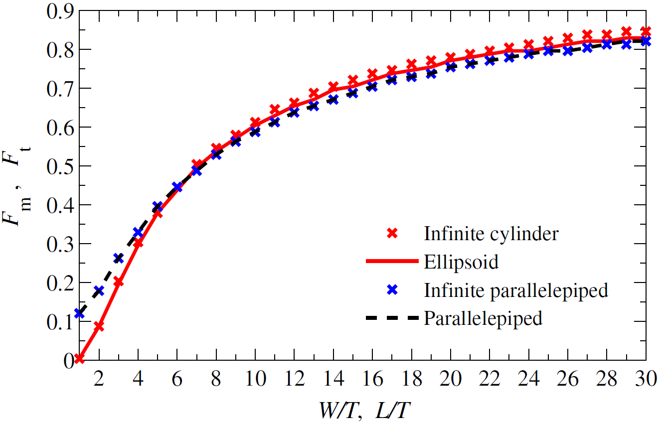
Figure 2: The modal filamentarity $F_{\mathrm{m}}$ versus $W/T$ and the truncation filamentarity $F_{\mathrm{t}}$ versus $L/T$. $F_{\mathrm{m}}$ is the value of $F$ where $\mathcal{P}(F)$ is maximum, and $F_{\mathrm{t}}$ where $\mathcal{P}(F)$ is truncated for finite-length structures. Results for elliptical and rectangular-base cylinders of finite length are shown with curves (solid/red and dashed/blue, respectively), those for shapes of infinite length are shown with crosses. The curves representing $F_{\mathrm{m}}$ and $F_{\mathrm{t}}$ for similar shapes overlap perfectly. The difference between the curves near the origin is due to the difference between a circle and a square.

3 Ellipsoids, from filaments to pancakes

We start with the simplest case of ideal filaments represented by a sample of randomly oriented, infinitely long elliptical cylinders with the base axis lengths $W$ and $T$. The probability density of the filamentarity in a randomly chosen cross-section of the sample, ${\mathcal{P}}(F)$, is shown in Fig. 1 for various values of $W/T$. The PDF has a single sharp, cuspy maximum at a certain $F=F_{\mathrm{m}}$ (called the modal value of $F$) that depends on $x=W/T$ as in Eq. (3) or Fig. 2 for $1\leq x<\infty$ since $W/T\geq 1$ by definition.

The filamentarity PDF has distinct asymptotic behaviours, also sensitive to $W/T$: exponential for $F\to 0$ and a power law at $F\to 1$. We do not present the corresponding fits here as they may be model dependent. We also considered infinite and finite cylinders with a rectangular base to obtain similar results but with $\mathcal{P}=0$ for $F<0.12$.

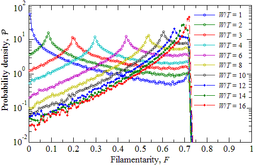
Figure 3: As Fig. 1, but for 200,000 random cuts of triaxial ellipsoids with $L/T=16$.

The effect of a finite length of the structure should be the strongest when the cross-section is nearly aligned with the structure’s major axis, i.e., at large $F$. This expectation is corroborated by Fig. 3 obtained for triaxial ellipsoids with fixed $L/T=16$ and various widths, $1\leq W/T\leq 16$. Unlike the case of an infinite cylinder shown in Fig. 1, the PDF of Fig. 3 is truncated: ${\mathcal{P}}=0$ at $F>F_{\mathrm{t}}\approx 0.73$ (the filamentarity of an ellipse with the axis ratio 16). The truncation filamentarity $F_{\mathrm{t}}$ provides a direct measure of $L/T$.

Comparison of Figs 1 and 3 shows that infinite cylinders and triaxial ellipsoids with the same $W/T$ have (nearly) the same modal filamentarity $F_{\mathrm{m}}$, so that Eq. (3) or Fig. 2 can be used to obtain $W/T$ from $F_{\mathrm{m}}$ in either case. Remarkably, the dependence of $F_{\mathrm{t}}$ on $L/T$ is identical to that of $F_{\mathrm{m}}$ on $W/T$, and both aspect ratios can be recovered from Eq. (3), or a similar equation for the ellipse, as it merely relates the relevant aspect ratio to the filamentarity.

The two most prominent aspects of the filamentarity PDF, its maximum and truncation, obtained from a single 2D cross-section provide complete, easily accessible information on the shape of the structures in 3D: both $W/T$ and $L/T$ can be recovered from $F_{\mathrm{m}}$ and $F_{\mathrm{t}}$, respectively, using Eq. (3) or its analogue for the ellipse.

As a circular filament ($W/T=1$, $L/T=16$) gradually turns into a pancake ($W/T=L/T=16$), $F_{\mathrm{m}}$ increases. This, perhaps counterintuitive, result can easily be understood: a large fraction of the random cuts of the filament are nearly circular ($F\approx 0$), whereas the majority of the pancake’s cuts are elongated.

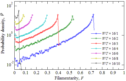
Figure 4: The filamentarity PDF for the cuts of oblate spheroids of $W=L=16$ and $T=1,2,3,4,6,8,10$, obtained from $\simeq 72,000$ individual cuts binned into $120$ intervals in $F$. Here, $F_{\mathrm{m}}=F_{\mathrm{t}}$.

4 Spheroids, from pancakes to spheres

For prolate spheroids ($W=T<L$), the PDF maximum is always at $F_{\mathrm{m}}=0$ (as one of the cuts is circular), so the left tail of $\mathcal{P}(F)$ disappears ($W/T=1$ in Fig. 3), but $F_{\mathrm{t}}$ remains the same function of $L/T$. For oblate spheroids ($T<W=L$), the modal and truncation filamentarities are the same, $F_{\mathrm{m}}=F_{\mathrm{t}}$, as shown with filled red circles ($W/T=16$) in Fig. 3 and, separately, in Fig. 4. As an oblate spheroid (pancake) gradually turns into a sphere, the maximum of the PDF shifts to the left, $F_{\mathrm{m}}\to 0$. The value of $F_{\mathrm{m}}$ immediately gives us the value of $W/T=L/T$ using Eq. (3).

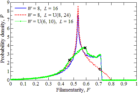
Figure 5: The filamentarity PDF for the cuts of triaxial ellipsoids of fixed shape $W/T=8$, $L/T=16$ (blue solid line); ellipsoids with a range of lengths, $W/T=8$, $L/T\sim U(8,24)$ (red dots); and ellipsoids with a range of widths, $L/T=16$, $W/T\sim U(6,10)$ (green dots) (288,000 realizations with $240$ bins in $F$).

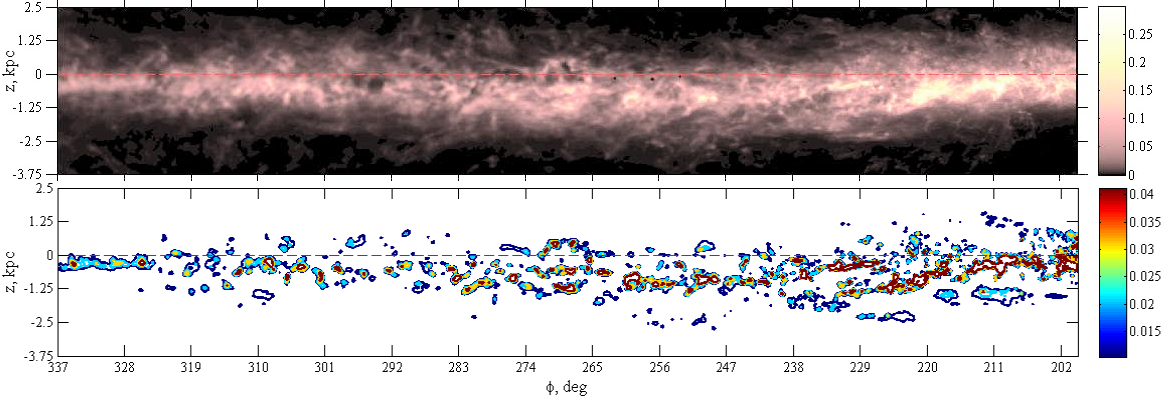
Figure 6: Upper panel: the H i number density (in cm^-3) from the GASS survey (Kalberla et al., 2010) at $r=16\,$kpc, $200^{\circ}\leq\phi\leq 337^{\circ}$, $-3.75<z<2.5\,{\rm kpc}$, with $(r,\phi,z)$ the Galactocentric cylindrical coordinates with the Sun at $(r,\phi,z)=(8.5\,\mathrm{kpc},180^{\circ},0$). Lower panel: The isocontours of the fluctuations $n$ in the gas number density obtained from the data of the upper panel. The mean value of $n$ is zero; the contours shown are at $n=\nu\sigma$, with $\nu=1,2,3,4,5$ and $\sigma=0.01\,\mathrm{cm}^{-3}$ the r.m.s. value of $n$ in this region.

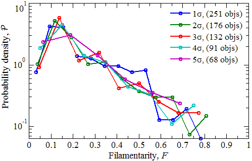
Figure 7: $\mathcal{P}(F)$ for a 2D cross-section of the fluctuations of neutral hydrogen density $n$ in the Milky Way at a Galactocentric radius $R=16\,{\rm kpc}$. Different curves refer to various levels, $n=\nu\sigma$ with $\sigma$ the r.m.s. value of $n$ and $\nu=1,2,\ldots 5$.

5 A range of shapes

Now, consider how $\mathcal{P}(F)$ changes when the ellipsoids have randomly distributed aspect ratios, conservatively chosen using uniform probability distributions. More localized distributions would have a weaker effect.

Figure 5 shows, with red filled circles, ${\mathcal{P}}(F)$ for ellipsoids of $W/T=8$ and $L/T$ uniformly distributed in the interval $L_{1}\leq L\leq L_{2}$, where $L_{1}/T=8$ and $L_{2}/T=24$, i.e., $L/T\sim U(8,24)$, with the mean value $\langle L/T\rangle=16$ and the standard deviation $\sigma_{L/T}=4.62$. The PDF maximum is at the same value of $F_{\mathrm{m}}$ and remains as sharp as for the fixed length $L/T=16$ (blue line in Fig. 5 and yellow, in Fig. 3), but the right tail of the PDF becomes longer and has an inflection point at $F_{\mathrm{i}}=0.71$ corresponding to $\langle L/T\rangle=16.5$ (provided $W<L_{1}$); the inflection point is marked with open circle. Thus, for ellipsoids with a range of lengths, the inflection point of ${\mathcal{P}}(F)$ is close to the value of $F$ where ${\mathcal{P}}$ is truncated for ellipsoids whose relative length is $\langle L/T\rangle$. The position of $F_{\mathrm{t}}$, such that ${\mathcal{P}}(F_{\mathrm{t}})=0$, provides a direct measure of the maximum length $L_{2}/T$: $F_{\mathrm{t}}\approx 0.8$ in Fig. 5, corresponding to $L_{2}/T\approx 24$ from Fig. 2 or Eq. (3). The extent of the right tail from the inflection point to $F_{\mathrm{t}}$ is proportional to $\sigma_{L}$: $F_{\mathrm{t}}-F_{\mathrm{i}}\approx 0.1\sigma_{L/T}$. Thus, Eq. (3) or a similar equation for ellipses can be used to determine the parameters of random-shape ellipsoids from the corresponding values of $F$.

The right tail of the PDF is slightly different when $W>L_{1}$: the inflection point disappears but $\log{\mathcal{P}}(F)$ still has it. Prolate spheroids with randomly distributed length ($T=W<L_{1}$) produce a similar picture: the truncation point gives $L_{2}/T$, and the inflection point gives $\langle L/T\rangle$.

A uniform distribution of the ellipsoid widths $W$ at fixed $T$ and $L$ has a stronger, but easily understandable, influence on the shape of the PDF. The peak, sensitive to $W/T$, becomes lower and broader (the green line in Fig. 5), but the most probable value of $F$ depends on the mean value of $W/T$ exactly as before. Its width (between the points marked with crosses on the green curve), $0.47\leq F_{\mathrm{m}}\leq 0.6$, reflects directly the range $6.5\lesssim W/T\lesssim 10.2$, using Eq. (3).

6 Galactic turbulence

The interstellar medium (ISM) of spiral galaxies is involved in transonic turbulent motions (Elmegreen & Scalo, 2004; Scalo & Elmegreen, 2004). As a result, the observed distribution of neutral hydrogen is dominated by filamentary structures which may be partially due to quasi-spherical shells viewed tangentially, and it remains unclear if the filaments are real or just an artifact of projection (Kulkarni & Heiles, 1988). Numerical simulations of the ISM also show filamentary structures produced by compression (Ballesteros-Paredes et al., 1999; Korpi et al., 1999). However, the morphology of the gas filaments has never been quantified in either observations or simulations.

The upper panel of Fig. 6 shows a cross-section of the fluctuations in the number density of neutral hydrogen, H i, in the Milky Way from the GASS survey (Kalberla et al., 2010) at a constant Galactocentric radius of 16 kpc. We have subtracted large-scale trends along and across the gas layer to obtain gas density fluctuations $n$ with vanishing mean value shown in the lower panel (Makarenko et al., in preparation).

The lower panel of Fig. 6 shows the isocontours of $n$. To ensure that contours obtained at various levels are not strongly correlated, they are separated in $n$ by its standard deviation $\sigma$, $n=\nu\sigma$ with integer $\nu$. The filamentarity of individual contours in Fig. 6 was obtained using Eq. (1) from their enclosed areas and perimeters measured directly in the image (essentially by counting pixels within a contour and on its boundary), without approximating them as ellipses (or any other shapes).

The PDFs of the filamentarity of the contours of Fig. 6 are shown in Fig 7. The PDFs at all levels are remarkably similar. This suggests a self-similar shape of the isodensity surfaces in this range of $\nu$. The PDFs are all similar to those of triaxial ellipsoids as they have a well pronounced maximum (note the logarithmic scale of the vertical axis), a power-law tail at larger $F$ and a clear truncation that occurs at the same $F$ for all the isosurface levels; in particular, none of about 700 structures discernible in the lower panel of Fig. 6 has $F$ exceeding approximately 0.8. The form of the PDF indicates that the H i distribution is indeed filamentary in 3D (compare Figs 7 and 3). The locations of the maximum at $F_{\mathrm{m}}=0.10$–0.15 and truncation at $F_{\mathrm{t}}=0.7$–0.8 yield, using Eq. (3), the mean width of the filaments as $W/T=2$–3 and their largest length as $L_{2}/T\approx 15$–25.

The scatter of the curves in Fig. 7 provides a measure of the errors involved. For example, the most probable value of $F$ varies in the range $0.09<F_{\mathrm{m}}<0.16$ for $1\geq\nu\geq 4$, leading to an uncertainty of $\pm 0.3$ in $W/T$. The value of $F_{\mathrm{t}}$ might be affected by insufficient statistics as it is obtained from the low-probability tail of $\mathcal{P}(F)$. Although $\mathcal{P}(F_{\mathrm{t}})\simeq 0.1\text{--}0.2$ is reasonably high, further analysis is required. The accuracy of the results can be improved by combining several cross-sections but we leave this to a detailed analysis of the H i density fluctuations which will be published elsewhere.

7 What can be learned from the filamentarity PDF?

The probability density function $\mathcal{P}$ of the filamentarity $F$ of the individual structures in a 2D cross-section of a 3D sample of isotropically oriented triaxial ellipsoids is a sensitive diagnostic of the 3D morphology of the ellipsoids.

If all the ellipsoids have the same axis ratios $W/T$ and $L/T$ (but not necessarily the same size):

1. ${\mathcal{P}}(F)$ has a single sharp maximum at $F=F_{\mathrm{m}}$, and $F_{\mathrm{m}}$ is related uniquely and simply to $x=W/T$ as given by Eq. (3) and shown in Fig. 2.

2. For structures of finite length, ${\mathcal{P}}=0$ for $F>F_{\mathrm{t}}$, and $F_{\mathrm{t}}$ depends on $L/T$ exactly as $F_{\mathrm{m}}$ depends on $W/T$.

3. Non-zero probability at $F\to 0$ indicates that the ellipsoids have a circular cross-section.

4. Non-zero probability at $F\to 1$ indicates that the length of the ellipsoids is comparable to or exceeds the size of the volume sampled, so that they are effectively infinitely long.

5. When $F_{\mathrm{m}}=F_{\mathrm{t}}$, the structures are oblate spheroids. The closer $F_{\mathrm{m}}$ is to zero, the closer the objects are to spheres.

6. When $F_{\mathrm{m}}=0$, the structures are prolate spheroids.

We have also considered the effect of randomly distributed $W/T$ and $L/T$, i.e., random structures of variable shape. For the width and length uniformly distributed over the ranges $W_{1}<W<W_{2}$ and $L_{1}<L<L_{2}$, we have shown that:

1. The maximum of ${\mathcal{P}}$ at $F=F_{\mathrm{m}}$ becomes flatter and loses a cusp, but its position depends on the mean value of $W$ exactly as above. The width of the maximum is related to the range of $W$.

2. The abrupt truncation of ${\mathcal{P}}$ at larger $F$ is replaced by a range of $F$ where ${\mathcal{P}}$ decreases smoothly before being truncated. Now, ${\mathcal{P}}(F)$ acquires an inflection point at $F=F_{\mathrm{i}}$ corresponding to the mean value of $L/T$. The eventual truncation to ${\mathcal{P}}=0$ occurs at $F=F_{\mathrm{t}}$ that uniquely depends on $L_{2}/T$, and $F_{\mathrm{t}}-F_{\mathrm{i}}$ is proportional to $L_{2}-L_{1}$.

Altogether, the PDF of the filamentarity in a 2D cross-section provides remarkably rich and easily accessible information about the morphology of the 3D random structures which can be recovered from a single, simple dependence of Eq. (3) or its analogue for ellipses. Anisotropic structure distributions produce a secondary maximum in ${\mathcal{P}}(F)$, which can be used to characterize the anisotropy as will be discussed elsewhere.

We have demonstrated the efficiency of this approach to morphological analysis using isosurfaces of the density fluctuations in the compressible, turbulent interstellar gas in the Milky Way. We have confirmed that the structures visible in a 2D cross-section of the isosurfaces are consistent with isotropically distributed filaments (rather than shells or other flattened objects) and estimated, for the first time, the relative width and length of the filamentary structures.

References

- Adler & Taylor (2007) Adler R. J., Taylor J. E., 2007, Random Fields and Geometry. Springer, New York
- Ballesteros-Paredes et al. (1999) Ballesteros-Paredes J., Vázquez-Semadeni E., Scalo J., 1999, ApJ, 515, 286
- Elmegreen & Scalo (2004) Elmegreen B. G., Scalo J., 2004, ARA&A, 42, 211
- Kalberla et al. (2010) Kalberla P. M. W., McClure-Griffiths N. M., Pisano D. J., Calabretta M. R., Ford H. A., Lockman F. J., Staveley-Smith L., Kerp J., Winkel B., Murphy T., Newton-McGee K., 2010, A&A, 521, A17
- Korpi et al. (1999) Korpi M. J., Brandenburg A., Shukurov A., Tuominen I., Nordlund Å., 1999, ApJ, 514, L99
- Kulkarni & Heiles (1988) Kulkarni S. R., Heiles C., 1988, in Kellermann K. I., Verschuur G. L., eds, Galactic and Extragalactic Radio Astronomy. Springer, New York, p. 95
- Mecke et al. (1994) Mecke K. R., Buchert T., Wagner H., 1994, A&A, 288, 697
- Platzöder & Buchert (1996) Platzöder M., Buchert T., 1996, in Weiss A., Raffelt G., Hillebrandt W., von Feilitzsch F., Buchert T., eds, Proc. 1st SFB Workshop, Astro-Particle Physics. Technische Universität, Münich, p. 251
- Rivollier et al. (2010) Rivollier S., Debayle J., Pinoli J. C., 2010, Aust. J. Math. Anal. Appl., 7, 1
- Rybicki (1987) Rybicki G. B., 1987, in de Zeeuw P. T., ed., Proc. IAU Symp. 127, Structure and Dynamics of Elliptical Galaxies. D. Reidel, Dordrecht, p. 397
- Sahni et al. (1998) Sahni V., Sathyaprakash B. S., Shandarin S. F., 1998, ApJ, 495, L5
- Scalo & Elmegreen (2004) Scalo J., Elmegreen B. G., 2004, ARA&A, 42, 275
- Schmalzing et al. (1999) Schmalzing J., Buchert T., Melott A. L., Sahni V., Sathyaprakash B. S., Shandarin S. F., 1999, ApJ, 526, 568
- Schneider & Weil (2008) Schneider R., Weil W., 2008, Stochastic and Integral Geometry. Springer, Berlin
- Vinci et al. (2014) Vinci G., Freeman P., Newman J., Wasserman L., Genovese C., 2014, in Statistical Challenges in the 21st Century Cosmology, IAU Symp. 306. Cambridge Univ. Press, Cambridge (in press; arXiv: 1406.7536)
- Wiegand et al. (2014) Wiegand A., Buchert T., Ostermann M., 2014, MNRAS, 443, 241