Probing non-perturbative effects in M-theory

Abstract

The AdS/CFT correspondence enables us to probe M-theory on various backgrounds from the corresponding dual gauge theories. Here we investigate in detail a three-dimensional $U(N)$ $\mathcal{N}=4$ super Yang-Mills theory coupled to one adjoint hypermultiplet and $N_{f}$ fundamental hypermultiplets, which is large $N$ dual to M-theory on $AdS_{4}\times S^{7}/\mathbb{Z}_{N_{f}}$. Using the localization and the Fermi-gas formulation, we explore non-perturbative corrections to the partition function. As in the ABJM theory, we find that there exists a non-trivial pole cancellation mechanism, which guarantees the theory to be well-defined, between worldsheet instantons and membrane instantons for all rational (in particular, physical or integral) values of $N_{f}$.

1 Introduction

In this paper, we study non-perturbative aspects of M-theory via the AdS/CFT correspondence Maldacena:1997re . Our analysis here is based on the belief that the AdS/CFT correspondence (or more generally, the gauge/gravity duality) is exactly true even at quantum level. This means that gauge theories, if they have gravity duals, provide us a “non-perturbative definition” of their dual string theories/M-theory on the corresponding backgrounds. Recent remarkable developments on exact understandings of gauge theories enable us to probe the non-perturbative effects in the dual string theories/M-theory, quantitatively.

We are interested in the low energy effective theories on multiple M2-branes, which have a dual M-theory description on some $AdS_{4}$ background. The most well-known example is a $U(N)_{k}\times U(N)_{-k}$ $\mathcal{N}=6$ supersymmetric Chern-Simons-matter theory, known as the ABJM theory ABJM . The ABJM theory describes the low energy effective theory on the $N$ M2-branes probing a $\mathbb{C}^{4}/\mathbb{Z}_{k}$ singularity, and it is dual to M-theory on $AdS_{4}\times S^{7}/\mathbb{Z}_{k}$ in the large $N$ limit. In this paper, we pick up another example: a three-dimensional $U(N)$ $\mathcal{N}=4$ super Yang-Mills theory coupled to one adjoint hypermultiplet and $N_{f}$ fundamental hypermultiplets. This theory also describes the theory on $N$ M2-branes probing a $\mathbb{C}^{2}\times\mathbb{C}^{2}/\mathbb{Z}_{N_{f}}$ singularity Benini:2009qs . From the Type IIA viewpoint, this is the worldvolume theory on $N$ D2-branes in the presence of $N_{f}$ D6-branes. This theory is dual to M-theory on $AdS_{4}\times S^{7}/\mathbb{Z}_{N_{f}}$ in the limit $N\to\infty$ with $N_{f}$ fixed. Note that the $\mathbb{Z}_{N_{f}}$ quotient on $S^{7}$ acts differently from the ABJM case. We can probe M-theory from these theories via the AdS/CFT correspondence. We would like to find universal (background independent) properties in M-theory through various examples.

As shown in KWY1 ; Jafferis:2010un ; Hama:2010av , in many supersymmetric gauge theories on $S^{3}$, infinite dimensional path integrals for the partition function and vacuum expectation values (VEVs) of BPS Wilson loops reduce to finite dimensional matrix integrals by using the localization technique. Due to this drastic simplification, one can, in principle, evaluate the partition function and the Wilson loop VEVs beyond the perturbation theory. However, it is still non-trivial to extract their large $N$ behaviors from the matrix integrals. The traditional matrix model technique is very helpful in the analysis in the ’t Hooft limit. In the ABJM matrix model, a systematic analysis in the ’t Hooft limit was done in MP1 ; DMP1 . However it is not easy to access the M-theory regime in this way (see Herzog:2010hf ). It is desirable to find more efficient ways to understand the M-theory regime systematically.

Recently, Mariño and Putrov proposed a very interesting formulation, known as the Fermi-gas approach, to analyze matrix models for a wide class of 3d Chern-Simons-matter theories MP2 . This Fermi-gas approach was successfully applied to the ABJM theory and revealed a very detailed structure of the non-perturbative effects in M-theory. It turned out that the existence of two types of instantons, i.e. worldsheet instantons and membrane instantons, is crucial for the non-perturbatively complete definition of the theory. In particular, the worldsheet instanton correction diverges at every physical value of the coupling, and that divergence is precisely canceled by the similar, but opposite sign, divergence of the membrane instanton correction HMO2 . This pole cancellation mechanism is conceptually very important, since this mechanism guarantees that we can go smoothly from the weak coupling (Type IIA) regime to the strong coupling (M-theory) regime. More practically, this mechanism gives strong constraint on the possible form of membrane instantons. For the ABJM case, we can actually find the analytic form of a first few membrane instanton coefficients using this pole cancellation condition, together with some other input from the semi-classical expansion of Fermi-gas HMO2 ; CM ; HMO3 . Based on these analytic results, it was finally found in HMMO ; KM that the membrane instantons in the ABJM theory are completely determined by the refined topological string on local $\mathbb{P}^{1}\times\mathbb{P}^{1}$, in the Nekrasov-Shatashvili limit Nekrasov:2009rc , while the worldsheet instantons are given by the standard topological string on the same manifold DMP1 ; HMO2 . In addition, there are bound states of membrane instantons and worldsheet instantons, whose contributions are finally absorbed into the worldsheet instanton corrections by the effective shift of chemical potential of the Fermi-gas system HMO3 . In the ABJ theory ABJ , the similar structure was also found MM ; HO ; Kallen:2014lsa based on the results Awata:2012jb ; Honda:2013pea .

In the present paper, we will study the $S^{3}$ partition function $Z(N_{f},N)$ of the $U(N)$ $\mathcal{N}=4$ super Yang-Mills theory coupled to one adjoint hypermultiplet and $N_{f}$ fundamental hypermultiplets. Using the localization technique, the computation of $Z(N_{f},N)$ boils down to a matrix integral, which was named as the $N_{f}$ matrix model in GM . It is known that the grand partition function of the $N_{f}$ matrix model can be recast as a Fermi-gas system, and some of its properties were studied in Mezei:2013gqa ; GM . This $N_{f}$ matrix model is an interesting first step beyond ABJ(M) theory to study the non-perturbative effects in M-theory. However, it turned out that it is not straightforward to apply the strategy in the previous paragraph, which was successful in the ABJM case HMO2 , to the $N_{f}$ matrix model:

1. Find the worldsheet instanton coefficients and their pole structure.

2. Determine the analytic form of the membrane instanton correction by combining the small $N_{f}$ expansion and the pole cancellation condition.

At the step 1, in the case of ABJM theory, the analytic form of the worldsheet instanton correction is available thanks to the relation to the topological string on local $\mathbb{P}^{1}\times\mathbb{P}^{1}$. On the other hand, the $N_{f}$ matrix model does not seem to have a direct connection to the topological string theory, and hence the analytic form of the worldsheet instanton correction is not known, except for the genus zero part GM . Currently, there is no systematic way to compute the worldsheet instanton corrections as analytic functions of $N_{f}$. To overcome this problem, we first compute the exact values of the partition function $Z(N_{f},N)$ for various integral values of $N_{f}$ up to some high $N$, and then guess the worldsheet instanton coefficients as functions of $N_{f}$ using the exact data of $Z(N_{f},N)$. In this way, we indeed find the analytic forms of worldsheet instanton coefficients up to three-instanton (3.24). We note that our conjecture gives an all-genus prediction in each instanton sector when taking the ’t Hooft limit. Our conjecture passes many non-trivial checks.

The small $N_{f}$ expansion at step 2 is also difficult to be carried out, since the density matrix (or Hamiltonian) of the Fermi-gas explicitly depends on $N_{f}$ Mezei:2013gqa ; GM . Nevertheless, we successfully find the first few terms of the small $N_{f}$ expansion of the grand potential by analyzing the so-called thermodynamic Bethe ansatz (TBA) equations. Combining the small $N_{f}$ expansion and the pole cancellation condition, we determine the membrane one-instanton coefficient completely (4.34) and find a part of the membrane two-instanton coefficients (4.39), as analytic functions of $N_{f}$. As a non-trivial check, we show that our conjecture of membrane instantons is consistent with the numerical solution of the TBA equations for $0<N_{f}<1$. These results clearly show that the pole cancellation mechanism is a general phenomenon in M-theory, not the special property of the ABJ(M) theory.

This paper is organized as follows: In section 2, we review the known properties of the $N_{f}$ matrix model, including the Fermi-gas approach, the TBA equations, and the ’t Hooft and the M-theory limits of this model. In section 3, first we explain our algorithm to compute the exact values of the partition functions $Z(N_{f},N)$ for various integral values of $N_{f}$. Then, using these exact values, we analyze the structure of the grand potential. We find that the constant $A(N_{f})$ in the grand potential is related to the constant map contribution of the topological string. We also determine the analytic forms of the worldsheet instanton coefficients up to three-instanton. In section 4, we consider the membrane instanton corrections. First we study the small $N_{f}$ expansion of the TBA equations, then we consider the pole cancellation condition between the worldsheet instantons and the membrane instantons. Finally, combining these two inputs, we determine the analytic forms of the membrane one-instanton and of a part of the membrane two-instanton. Section 5 is the conclusion. We also have three appendices A, B, and C, summarizing some results used in the main text.

2 Review of Fermi-gas approach

Let us start by reviewing the exact computation of the partition function on $S^{3}$ by using the localization KWY1 and the Fermi-gas approach MP2 . The localization reduces the partition function to a finite dimensional matrix integral. We rewrite this matrix integral as a partition function of certain one-dimensional ideal Fermi-gas system as in MP2 . This approach is quite powerful, and allows us to analyze the non-perturbative corrections to the partition function.

2.1 From matrix model to Fermi-gas

In this paper we consider the $U(N)$ $\mathcal{N}=4$ super Yang-Mills theory on $S^{3}$ with one adjoint hypermultiplet and $N_{f}$ fundamental hypermultiplets. The quiver diagram for this theory is shown in figure 1(a). Following the general localization procedure in KWY1 , one can immediately write down the partition function of this theory, and the result is given by the matrix integral

$$Z(N_{f},N)=\frac{1}{N!}\int\prod_{j=1}^{N}\frac{dx_{j}}{4\pi}\frac{1}{(2\cosh\frac{x_{j}}{2})^{N_{f}}}\prod_{j<k}\tanh^{2}\left(\frac{x_{j}-x_{k}}{2}\right).$$ (2.1)

Our goal in this paper is to understand the large $N$ behavior of this model, the so-called $N_{f}$ matrix model, including non-perturbative corrections. We note that the matrix integral (2.1) can be evaluated for arbitrary value of $N_{f}$ while the physical theory is defined only for integral $N_{f}$. It is well-known that the theory with $N_{f}=1$ is equivalent to the ABJM theory at Chern-Simons level $k=1$ via the mirror symmetry ABJM . The equality of the partition functions of both theories was directly shown in KWY2 . Interestingly, the partition function for $N_{f}=2$ is also related to the partition function of the $U(N)_{k}\times U(N+1)_{-k}$ ABJ theory at $k=2$

$$|Z_{\rm ABJ}(k=2,N,N+1)|=\frac{1}{\sqrt{2}}Z(N_{f}=2,N),$$ (2.2)

where the factor $1/\sqrt{2}$ comes from the partition function of $U(1)_{k=2}$ pure Chern-Simons theory. This relation can be checked by rewriting the ABJ partition function as in HO . The quiver diagram of the ABJ(M) theory is shown in figure 1(b).

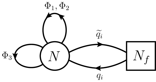
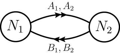
(a)	(b)

Figure 1: (a) The quiver diagram for the $U(N)$ $\mathcal{N}=4$ SYM with an adjoint and $N_{f}$ fundamental hypermultiplets. We use $\mathcal{N}=2$ notation. The adjoint hypermultiplet consists of two adjoint chiral multiplets $(\Phi_{1},\Phi_{2})$, and $\Phi_{3}$ is the chiral multiplet that forms the $\mathcal{N}=4$ vector multiplet together with the $\mathcal{N}=2$ vector multiplet. (b) The quiver for the $U(N_{1})_{k}\times U(N_{2})_{-k}$ ABJ(M) theory. The partition function of the former with $N_{f}=1,2$ is related to that of the latter at $k=1,2$, respectively.

It is not easy to perform the matrix integral (2.1) directly. However, there is a very efficient way to compute the exact values of the partition function. This method was first proposed in MP2 (see also Okuyama:2011su ), and is now called the Fermi-gas approach. The key idea is to rewrite the partition function (2.1) as

$$Z(N_{f},N)=\frac{1}{N!}\sum_{\sigma\in S_{N}}(-1)^{\sigma}\int\!d^{N}x\prod_{j=1}^{N}\rho(x_{j},x_{\sigma(j)}),$$ (2.3)

where

$$\rho(x_{1},x_{2})=\frac{1}{2\pi}\frac{1}{(2\cosh\frac{x_{1}}{2})^{N_{f}/2}}\frac{1}{(2\cosh\frac{x_{2}}{2})^{N_{f}/2}}\frac{1}{2\cosh\left(\frac{x_{1}-x_{2}}{2}\right)}.$$ (2.4)

To derive (2.3), we used the Cauchy determinant formula. The partition function (2.3) can be interpreted as the partition function of an ideal Fermi-gas system described by the density matrix $\rho$ MP2 . In the following analysis, it is very convenient to introduce the grand canonical partition function and the grand potential

$$\Xi(N_{f},z)=1+\sum_{N=1}^{\infty}z^{N}Z(N_{f},N),\qquad J(N_{f},\mu)=\log\Xi(N_{f},z),$$ (2.5)

where $z=e^{\mu}$ is a fugacity with a chemical potential $\mu$ in the grand canonical ensemble. As was discussed in MP2 , for the partition function with the form (2.3), the grand partition function is written as a Fredholm determinant

$$\Xi(N_{f},z)=\det(1+z\rho)=\exp\biggl{[}-\sum_{n=1}^{\infty}\frac{(-z)^{n}}{n}\operatorname{Tr}\rho^{n}\biggr{]},$$ (2.6)

where the trace of $\rho$ is defined by

$$\operatorname{Tr}\rho^{n}=\int_{-\infty}^{\infty}dx_{1}\cdots dx_{n}\,\rho(x_{1},x_{2})\rho(x_{2},x_{3})\cdots\rho(x_{n},x_{1}).$$ (2.7)

Therefore the basic problem is how to compute $\operatorname{Tr}\rho^{n}$. This is still not easy, but as will be seen in the next section, we can compute it recursively. Once we know the grand potential $J(N_{f},\mu)$, it is easy to reconstruct the canonical partition function by

$$Z(N_{f},N)=\int_{-\pi i}^{\pi i}\frac{d\mu}{2\pi i}e^{J(N_{f},\mu)-N\mu}.$$ (2.8)

2.2 TBA equations

The density matrix $\rho$ takes the form

$$\rho(x_{1},x_{2})=\frac{1}{2\pi}\frac{e^{-\frac{1}{2}U(x_{1})-\frac{1}{2}U(x_{2})}}{2\cosh\left(\frac{x_{1}-x_{2}}{2}\right)},\qquad U(x)=N_{f}\log\left[2\cosh\frac{x}{2}\right].$$ (2.9)

Interestingly, for the kernel with this form, we can compute the grand potential from the TBA equations Zamolodchikov:1994uw . The TBA integral equations are given by

$$\log R_{+}(x) =-U(x)+\int_{-\infty}^{\infty}\frac{dx^{\prime}}{2\pi}\frac{\log(1+\eta^{2}(x^{\prime}))}{\cosh(x-x^{\prime})},$$ (2.10)

$$\eta(x) =-z\int_{-\infty}^{\infty}\frac{dx^{\prime}}{2\pi}\frac{R_{+}(x^{\prime})}{\cosh(x-x^{\prime})}.$$

For the solutions of these equations, we also define

$$R_{-}(x)=R_{+}(x)\int_{-\infty}^{\infty}\frac{dx^{\prime}}{\pi}\frac{\arctan\eta(x^{\prime})}{\cosh^{2}(x-x^{\prime})}.$$ (2.11)

Once these functions are determined, the grand potential is computed by

$$\frac{\partial J_{\pm}}{\partial z}=\frac{1}{4\pi}\int_{-\infty}^{\infty}dx\,R_{\pm}(x),\qquad J_{\pm}(z)=\frac{J(z)\pm J(-z)}{2}.$$ (2.12)

We note that the integral equations (2.10) and (2.11) can be recast as the following functional relations CM , called the Y-system in the literature,

$$R_{+}\left(x+\frac{\pi i}{2}\right)R_{+}\left(x-\frac{\pi i}{2}\right)\exp\left[U\left(x+\frac{\pi i}{2}\right)+U\left(x-\frac{\pi i}{2}\right)\right] =1+\eta^{2}(x),$$ (2.13)

$$\eta\left(x+\frac{\pi i}{2}\right)+\eta\left(x-\frac{\pi i}{2}\right) =-zR_{+}(x),$$

and

$$\frac{R_{-}(x+\frac{\pi i}{2})}{R_{+}(x+\frac{\pi i}{2})}-\frac{R_{-}(x-\frac{\pi i}{2})}{R_{+}(x-\frac{\pi i}{2})}=2i\frac{\eta^{\prime}(x)}{1+\eta^{2}(x)}.$$ (2.14)

The TBA equations (2.10) and (2.11) are powerful in the numerical computation for various values of $N_{f}$ as in HMO1 . The functional equations (2.13) and (2.14), on the other hand, are useful in the semi-classical analysis CM . The TBA equations for the ABJM case were studied in HMO1 ; PY ; CM .

2.3 ’t Hooft limit and M-theory limit

We want to understand the large $N$ behavior of the partition function (2.1) (or equivalently (2.3)). There are two interesting limits. One is the standard ’t Hooft limit, in which the parameters are taken as follows:

$$N\to\infty,\qquad N_{f}\to\infty,\qquad\lambda=\frac{N}{N_{f}}\text{ : fixed},$$ (2.15)

where $\lambda$ is the ’t Hooft coupling. In this limit, the free energy admits the perturbative genus expansion (plus non-perturbative contribution)

$$F(g_{s},\lambda)=-\log Z(N_{f},N)=\sum_{g=0}^{\infty}g_{s}^{2g-2}F_{g}(\lambda)+F_{\text{np}}(g_{s},\lambda),\qquad g_{s}=\frac{1}{N_{f}},$$ (2.16)

where $F_{g}(\lambda)$ is the genus $g$ contribution, and $F_{\text{np}}(g_{s},\lambda)$ is the non-perturbative correction in $g_{s}$. In the ABJM matrix model, the genus zero contribution was computed by the standard matrix model technique, and the higher genus corrections were determined from the holomorphic anomaly equations MP1 ; DMP1 . In the $N_{f}$ matrix model, the genus zero contribution was computed in GM . However, it is difficult to compute the higher genus correction. The non-perturbative correction $F_{\text{np}}(g_{s},\lambda)$ is also very difficult to be computed from the usual matrix model approach. Some interesting results on the non-perturbative corrections in the ABJM matrix model are found in DMP2 ; Grassi:2014cla . We emphasize that the Fermi-gas approach overcomes this difficulty, and we can predict analytic results for $F_{\text{np}}(g_{s},\lambda)$. One important consequence is that the perturbative genus expansion is insufficient in the finite $g_{s}$ regime, and the existence of the non-perturbative contribution $F_{\text{np}}(g_{s},\lambda)$ is essential for the consistency of the theory.

We note that the genus $g$ contribution $F_{g}(\lambda)$ at strong coupling contains the non-perturbative corrections in $\alpha^{\prime}(\sim 1/\sqrt{\lambda})$, which has the exponentially suppressed contribution (see GM for the genus zero contribution)

$$\mathcal{O}(e^{-2\pi\sqrt{2\lambda}}).$$ (2.17)

From the dual Type IIA string point of view, such corrections are caused by the worldsheet instanton wrapping a two-cycle. On the other hand, the non-perturbative part $F_{\text{np}}(g_{s},\lambda)$ contains the exponentially suppressed contribution

$$\mathcal{O}(e^{-\pi\sqrt{2\lambda}/g_{s}}).$$ (2.18)

As discussed in DMP2 , such non-perturbative corrections come from the D2-branes wrapping a three-cycle. In this paper, we refer these corrections to the membrane instanton corrections because these are purely non-perturbative effects in $g_{s}$.

The other interesting limit is the following one:

$$N\to\infty,\qquad N_{f}\text{ : fixed},$$ (2.19)

corresponding to a direct thermodynamic limit of the Fermi-gas system. In this limit, the gauge theory is dual to M-theory on $AdS_{4}\times S^{7}/\mathbb{Z}_{N_{f}}$, and thus we call this limit as the M-theory limit here. In the following analysis, we mainly focus on the M-theory limit. In the M-theory limit, the worldsheet instanton correction (2.17) and the membrane instanton correction (2.18) have the same order

$$\mathcal{O}(e^{-2\pi\sqrt{2N/N_{f}}}),\qquad\mathcal{O}(e^{-\pi\sqrt{2N_{f}N}}).$$ (2.20)

This is because, in the M-theory regime, both instantons are up-lifted to M2-branes wrapping two different types of three-cycles. See figure 1 in HMMO for more detail.

Before closing this section, let us comment on the large $N$ limit in the grand canonical ensemble. From the integral transformation (2.8), the partition function can be evaluated by the saddle point approximation in the large $N$ limit. The saddle point equation is given by

$$J^{\prime}(\mu_{*})-N=0.$$ (2.21)

As was discussed in Mezei:2013gqa ; GM , the grand potential behaves in the large $\mu$ limit as

$$J(N_{f},\mu)\approx\frac{2}{3\pi^{2}N_{f}}\mu^{3}\qquad(\mu\to\infty).$$ (2.22)

Therefore, the saddle point is given by

$$\mu_{*}=\pi\sqrt{\frac{N_{f}N}{2}}.$$ (2.23)

This means that the large $N$ limit in the canonical ensemble corresponds to the large $\mu$ limit in the grand canonical ensemble. The saddle point analysis presents a simple derivation of the $N^{3/2}$ behavior of the free energy MP2

$$F(N_{f},N)\approx-J(N_{f},\mu_{*})+N\mu_{*}\approx\frac{\pi\sqrt{2N_{f}}}{3}N^{3/2}\qquad(N\to\infty).$$ (2.24)

This reproduces the matrix model result Mezei:2013gqa . As we will see later, the Airy function behavior is also derived easily from the grand canonical analysis. Finally, the worldsheet instanton correction and the membrane instanton correction in (2.20) correspond to the exponentially suppressed corrections

$$\mathcal{O}(e^{-4\mu/N_{f}}),\qquad\mathcal{O}(e^{-2\mu}),$$ (2.25)

respectively, in the grand canonical ensemble.

3 Exploring non-perturbative effects

In this section, we investigate the non-perturbative corrections to the partition function (2.1) in the large $N$ limit. As explained in the previous section, the large $N$ limit corresponds to the large $\mu$ limit in the grand canonical ensemble. We thus concentrate our attention on the large $\mu$ behavior of the grand potential. We first compute the exact values of the partition function for various integral $N_{f}$ by using the Fermi-gas approach developed in PY ; HMO1 ; HMO2 . Next, using these exact data, we extract the non-perturbative corrections to the grand potential. Based on these results, we look for exact forms of the worldsheet instanton corrections for general $N_{f}$. The membrane instanton corrections are explored in the next section.

3.1 Exact computation of the partition function

In this subsection, we compute the exact values of the partition function for some integral values of $N_{f}$. Our strategy is the same as that in the ABJM theory HMO1 ; HMO2 . We first divide the density matrix $\rho$ into parity even/odd part

$$\rho(x_{1},x_{2})=\rho_{+}(x_{1},x_{2})+\rho_{-}(x_{1},x_{2}),\quad\rho_{\pm}(x_{1},x_{2})=\frac{\rho(x_{1},x_{2})\pm\rho(x_{1},-x_{2})}{2}.$$ (3.1)

Then, the grand partition function is factorized into two parts HMO1 ,

$$\Xi(z)=\det(1+z\rho_{+})\det(1+z\rho_{-}).$$ (3.2)

As in HMO1 ; HMO2 , we write $\rho_{\pm}$ as the forms

$$\rho_{\pm}(x,y)=\frac{E_{\pm}(x)E_{\pm}(y)}{\cosh x+\cosh y},$$ (3.3)

where

$$E_{+}(x)=\frac{\cosh\frac{x}{2}}{(2\cosh\frac{x}{2})^{N_{f}/2}},\qquad E_{-}(x)=\frac{\sinh\frac{x}{2}}{(2\cosh\frac{x}{2})^{N_{f}/2}}.$$ (3.4)

Now we can apply the result in TW to the kernels $\rho_{\pm}$. The important consequence is that we can compute $\rho_{\pm}^{n}$ from functions with one variable:

$$\rho_{\pm}^{2n+1}(x,y) =\frac{E_{\pm}(x)E_{\pm}(y)}{\cosh x+\cosh y}\sum_{\ell=0}^{2n}(-1)^{\ell}\phi_{\pm}^{\ell}(x)\phi_{\pm}^{2n-\ell}(y),$$ (3.5)

$$\rho_{\pm}^{2n}(x,y) =\frac{E_{\pm}(x)E_{\pm}(y)}{\cosh x-\cosh y}\sum_{\ell=0}^{2n-1}(-1)^{\ell}\phi_{\pm}^{\ell}(x)\phi_{\pm}^{2n-1-\ell}(y),$$

where the functions $\phi_{\pm}^{\ell}(x)$ are determined by the following integral equations recursively

$$\phi_{+}^{\ell}(x) =\frac{1}{\cosh\frac{x}{2}}\int_{-\infty}^{\infty}\frac{dx^{\prime}}{2\pi}\frac{1}{2\cosh\left(\frac{x-x^{\prime}}{2}\right)}\frac{\cosh\frac{x^{\prime}}{2}}{(2\cosh\frac{x^{\prime}}{2})^{N_{f}}}\phi_{+}^{\ell-1}(x^{\prime}),$$ (3.6)

$$\phi_{-}^{\ell}(x) =\frac{1}{\cosh\frac{x}{2}}\int_{-\infty}^{\infty}\frac{dx^{\prime}}{2\pi}\frac{1}{2\cosh\left(\frac{x-x^{\prime}}{2}\right)}\frac{\sinh\frac{x^{\prime}}{2}\tanh\frac{x^{\prime}}{2}}{(2\cosh\frac{x^{\prime}}{2})^{N_{f}}}\phi_{-}^{\ell-1}(x^{\prime}),$$

with the initial conditions $\phi_{\pm}^{0}(x)=1$. For a derivation of these equations, see HMO1 . In HMO1 ; HMO2 , we further found that the grand partition function is expressed only in terms of the even parity part:

$$\Xi(z)=\det(1-z^{2}\rho_{+}^{2})G(z),\qquad G(z)=\sum_{\ell=0}^{\infty}\phi_{+}^{\ell}(0)z^{\ell}.$$ (3.7)

This result is very useful in the practical computation. In summary, we first solve the integral equation (3.6) for $\phi_{+}^{\ell}(x)$ recursively. This can be done very efficiently by using the technique in PY ; HMO2 . We then compute $\operatorname{Tr}\rho_{+}^{2n}$ to know $\det(1-z^{2}\rho_{+}^{2})$ by using (3.5). We finally read off the coefficient of $z^{N}$ in (3.7) that is nothing but $Z(N_{f},N)$.

We have computed the exact values of $Z(N_{f},N)$ for $N_{f}=1,2,\dots,12,14,16$, up to certain values of $N$. Since the results are very complicated, we cannot write them down here. Instead, a set of ancillary files for these values readable in Mathematica is attached to this paper on arXiv. In figure 2, we show the free energy $F=-\log Z$ for $N_{f}=1,2,\dots,6$ as a function of $N^{3/2}$. The dots represent the exact values while the solid lines represent the leading Airy function behaviors given by (3.11). The exact values of the free energy indeed show the $N^{3/2}$ behaviors, and also a very good agreement with the Airy function (3.11) even for small $N$.

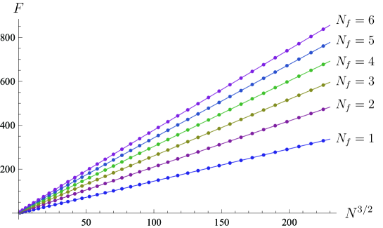
Figure 2: The free energy $F=-\log Z$ for $N_{f}=1,\dots,6$ as a function of $N^{3/2}$. The dots represent the exact values computed by our algorithm while the solid lines represent the perturbative part given by the Airy function (3.11).

3.2 General structure of the grand potential

Next we consider the structure of the grand potential. In the large $\mu$ limit, the grand potential takes the following form Mezei:2013gqa ; GM

$$J(N_{f},\mu)=\frac{C(N_{f})}{3}\mu^{3}+B(N_{f})\mu+A(N_{f})+J_{\text{np}}(N_{f},\mu)\qquad(\mu\to\infty),$$ (3.8)

where

$$C(N_{f})=\frac{2}{\pi^{2}N_{f}},\qquad B(N_{f})=\frac{1}{2N_{f}}-\frac{N_{f}}{8},$$ (3.9)

and $A(N_{f})$ is a non-trivial function of $N_{f}$. The remaining part $J_{\text{np}}(N_{f},\mu)$ is the exponentially suppressed correction in $\mu\to\infty$. As we have seen in the previous section, there are two such corrections, coming from the worldsheet instantons and the membrane instantons. In addition, there are also “bound states” of these two kinds of instantons CM . Taking into account of these bound states, the non-perturbative correction has the following expansion

$$J_{\text{np}}(N_{f},\mu)=\sum_{\begin{subarray}{c}\ell,m=0\\ (\ell,m)\neq(0,0)\end{subarray}}^{\infty}f_{\ell,m}(N_{f},\mu)\exp\left[-\left(2\ell+\frac{4m}{N_{f}}\right)\mu\right].$$ (3.10)

The structure is very similar to the ABJM case CM , but the explicit forms of the coefficients look quite different, as we will see later. The worldsheet instanton correction corresponds to $\ell=0$, and the membrane instanton correction to $m=0$. The others are understood as their bound states. If we ignore the non-perturbative correction $J_{\text{np}}(N_{f},\mu)$, the grand potential (3.8) leads to the following canonical partition function MP2

$$Z_{\text{pert}}(N_{f},N)=C(N_{f})^{-1/3}e^{A(N_{f})}\operatorname{Ai}\left[C(N_{f})^{-1/3}(N-B(N_{f}))\right].$$ (3.11)

where $\operatorname{Ai}(z)$ is the Airy function. This result is understood as the all-genus resummation after neglecting all the exponentially suppressed corrections FHM . Using the asymptotic expansion of the Airy function, one can, of course, reproduce the $N^{3/2}$ behavior (2.24) in the large $N$ limit.

Our remaining task is to determine the non-trivial functions $A(N_{f})$ and $f_{\ell,m}(N_{f},\mu)$. In the ABJ(M) theory, this program has already been done with the help of an accidental connection to the topological string on local $\mathbb{P}^{1}\times\mathbb{P}^{1}$ (see HMO2 ; CM ; HMO3 ; HMMO ; MM ; HO ). However, in our case of the $N_{f}$ matrix model, we do not know a nice connection to the topological string. Therefore we do not have any guiding principles to determine the non-perturbative corrections systematically, and it is challenging to understand $f_{\ell,m}(N_{f},\mu)$. To explore the non-perturbative effects, we here take the following strategy:

• Using the exact data computed in the previous subsection, we extract the non-perturbative corrections for various integral values of $N_{f}$.

• Based on these data, we conjecture the worldsheet instanton correction $f_{0,m}(N_{f},\mu)$ for general $N_{f}$ order by order.

• The (conjectured) worldsheet instanton correction diverges for some values of $N_{f}$. These singularities must be canceled by the other contributions because the theory is always well-defined. This pole cancellation mechanism was first found in the ABJM theory HMO2 . Using this mechanism, we can determine the pole structure of the membrane instanton correction. Combining this information with some other inputs, we fix the analytic forms of the membrane instanton corrections.

• The obtained results can be compared with the numerical results computed from the TBA equations in section 2 for various (non-integral) values of $N_{f}$. This comparison gives a highly non-trivial test of our conjecture.

Of course, the analytic forms of higher instanton corrections become very complicated, and it gets more and more difficult to determine them in this way. In this paper, following the above strategy, we indeed determine the worldsheet instanton correction up to $m=3$, and also the leading membrane instanton correction (and a part of the next-to-leading correction). So far, we cannot obtain any results on the bound states. This should be understood in the future work.

3.3 The constant part

Before proceeding to the instanton corrections, we give a conjecture of the exact form of $A(N_{f})$. We find that the constant part $A(N_{f})$ is exactly related to that in the ABJM theory as

$$A(N_{f})=\frac{1}{2}\left[A_{\text{const}}(N_{f})+A_{\text{const}}(1)N_{f}^{2}\right],$$ (3.12)

where $A_{\text{const}}(k)$ is the constant part appearing in the grand potential in the ABJM Fermi-gas MP2 . Although we do not have a proof of this conjecture, it passes many non-trivial tests as we will see below. Note that $A_{\text{const}}(k)$ corresponds to the constant map contribution in the topological string KEK . The small $k$ expansion of $A_{\text{const}}(k)$ was first computed in MP2 , and then the all-loop formula and its integral expression were conjectured in KEK . As derived in appendix A, we find another simpler integral expression of $A_{\text{const}}(k)$:

$$A_{\text{const}}(k)=\frac{2\zeta(3)}{\pi^{2}k}\left(1-\frac{k^{3}}{16}\right)+\frac{k^{2}}{\pi^{2}}\int_{0}^{\infty}dx\frac{x}{e^{kx}-1}\log(1-e^{-2x}).$$ (3.13)

In particular, we find closed form expressions for any integer $k$,

$$A_{\text{const}}(k)=\begin{cases}\displaystyle-\frac{\zeta(3)}{\pi^{2}k}-\frac{2}{k}\sum_{m=1}^{\frac{k}{2}-1}m\left(\frac{k}{2}-m\right)\log\left(2\sin\frac{2\pi m}{k}\right)&(\text{even }k),\\ \displaystyle-\frac{\zeta(3)}{8\pi^{2}k}+\frac{k}{4}\log 2-\frac{1}{k}\sum_{m=1}^{k-1}g_{m}(k)(k-g_{m}(k))\log\left(2\sin\frac{\pi m}{k}\right)\;&(\text{odd }k),\end{cases}$$ (3.14)

where

$$g_{m}(k)=\frac{k+(-1)^{m}(2m-k)}{4}.$$ (3.15)

Our conjecture (3.12) predicts the small $N_{f}$ expansion

$$A(N_{f})=\frac{\zeta(3)}{\pi^{2}N_{f}}-\frac{N_{f}}{24}+\left(-\frac{\zeta(3)}{16\pi^{2}}+\frac{\log 2}{8}\right)N_{f}^{2}-\frac{\pi^{2}N_{f}^{3}}{8640}+\mathcal{O}(N_{f}^{5}).$$ (3.16)

The leading term coincides with the result in GM . As we will see in section 4, the next-to-leading correction is reproduced from the TBA analysis. Also, in the large $N_{f}$ limit, we find

$$\lim_{N_{f}\to\infty}\frac{A(N_{f})}{N_{f}^{2}}=\frac{1}{8}\left(-\frac{\zeta(3)}{\pi^{2}}+\log 2\right)=0.07141916904....$$ (3.17)

This result also agrees with the constant term in the genus-zero free energy found in GM . In figure 3, we plot $A(N_{f})$ for finite $N_{f}$. The solid line is our conjecture, while the dots are the numerical values of $A(N_{f})$ extracted from the exact values of $Z(N_{f},N)$, where we estimated them by (see (3.11))

$$A(N_{f})\approx\log\left[\frac{Z^{\text{exact}}(N_{f},N)}{C(N_{f})^{-1/3}\operatorname{Ai}\left[C(N_{f})^{-1/3}(N-B(N_{f}))\right]}\right]\quad(N\gg 1),$$ (3.18)

for $N$ as large as possible. For example, in the case of $N_{f}=3$, we computed exact $Z(3,N)$ up to $N=53$. Using the estimation (3.18) for $N=53$, we find

$$A(3)\approx 0.60247027481429615744.$$ (3.19)

On the other hand, the exact value of $A(3)$ in (3.12) is

$$A(3)=-\frac{7\zeta(3)}{12\pi^{2}}+\frac{1}{6}\log\frac{512}{9}.$$ (3.20)

The difference is $\mathcal{O}(10^{-16})$, which is roughly the same order as the leading worldsheet instanton correction $\mathcal{O}(e^{-2\pi\sqrt{2N/N_{f}}})$. For other values of $N_{f}$, our conjecture (3.12) indeed show an agreement with the numerical estimation up to about $\mathcal{O}(e^{-2\pi\sqrt{2N/N_{f}}})$.

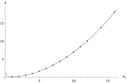
Figure 3: The constant contribution $A(N_{f})$. The numerical estimations (3.18) from exact $Z(N_{f},N)$ in the previous section are shown by the dots, and our conjecture (3.12) by the solid line.

3.4 Non-perturbative corrections for integral $N_{f}$

Using the exact values of the partition function computed in subsection 3.1, we can determine the non-perturbative correction to the grand potential. The basic method is the same as that in HMO2 . We first take an appropriate ansatz of the non-perturbative correction to the grand potential. We then pull it back to the canonical partition function. The coefficients in the ansatz are fixed by the numerical fitting of the exact values with high precision. See HMO2 in detail.

Since the partition function for $N_{f}=1,2$ is related to the ABJ(M) case, we can use the results in HMO2 ; HMO3 ; MM ; HO . We also find the corrections explicitly for $N_{f}=3,4,6,8,12$, and numerically for other $N_{f}$’s. We observe that all of these results take the form

$$J_{\text{np}}(N_{f},\mu)=\sum_{n=1}^{\infty}f_{n}(N_{f},\mu)e^{-\frac{4n\mu}{N_{f}}},\qquad N_{f}\in\mathbb{N}.$$ (3.21)

In particular, as in the ABJM case, the terms $e^{-(4m-2)\mu}$ ($m=1,2,\dots$) do not appear for odd $N_{f}$. The explicit forms of $f_{n}(N_{f},\mu)$ are complicated, and listed in appendix B.

3.5 Worldsheet instanton corrections

Now let us consider the worldsheet instanton correction

$$J^{\text{WS}}(N_{f},\mu)=\sum_{m=1}^{\infty}f_{0,m}(N_{f},\mu)e^{-\frac{4m\mu}{N_{f}}}.$$ (3.22)

Here we give a conjecture of the analytic form of $f_{0,m}(N_{f},\mu)$, which is valid for general $N_{f}$, up to $m=3$. To simplify the notation, we define

$$s_{n}(N_{f})=\sin\left(\frac{2\pi n}{N_{f}}\right),\qquad P_{n}(N_{f},\mu)=\frac{4n\mu+N_{f}}{\pi}.$$ (3.23)

Our conjecture of $f_{0,m}(N_{f},\mu)$ up to $m=3$ is

$$f_{0,1} =-\frac{1}{2s_{1}}P_{1},$$ (3.24)

$$f_{0,2} =-\frac{1}{4}P_{1}^{2}+\frac{3s_{3}}{8s_{1}s_{2}}P_{2}-\frac{s_{4}}{2s_{1}^{2}s_{2}},$$

$$f_{0,3} =-\frac{s_{2}^{2}}{12s_{1}}P_{1}^{3}+\frac{3s_{4}}{8s_{1}}P_{1}P_{2}-\frac{5s_{4}s_{5}}{9s_{1}s_{2}s_{3}}P_{3}-\frac{s_{4}^{2}}{2s_{1}s_{2}^{2}}P_{1}-\frac{2s_{6}}{s_{1}^{2}s_{3}}+\frac{2s_{4}s_{5}}{s_{1}^{2}s_{2}^{2}}.$$

We have checked that this conjecture is consistent with the exact values of $Z(N_{f},N)$ for $3\leq N_{f}\leq 16$. For $N_{f}=1,2$, worldsheet instantons (3.24) have poles already at the one-instanton level. We can also see that $f_{0,2}$ have poles at $N_{f}=1,2,4$ and $f_{0,3}$ have poles at $N_{f}=1,2,3,4,6.$ As we will see in the next section, those poles should be canceled by the membrane instantons.

One can check that our conjecture (3.24) correctly reproduces the result in appendix B. For instance, for $N_{f}=8$ we find

$$f_{0,1}(8,\mu) =-\frac{4\mu+8}{\sqrt{2}\pi},\quad f_{0,2}(8,\mu)=-\frac{(4\mu+8)^{2}}{4\pi^{2}}+\frac{3(4\mu+4)}{4\pi},$$ (3.25)

$$f_{0,3}(8,\mu) =-\frac{(4\mu+8)^{3}}{6\sqrt{2}\pi^{3}}+4\sqrt{2},$$

which agree with the result (B.6) in appendix B. Other cases in appendix B are also reproduced by the conjecture (3.24). We also stress that, for all other cases $N_{f}=5,7,9,\cdots,16$, our conjecture (3.24) agrees highly non-trivially with the instanton corrections extracted from the exact partition function. To see it, let us define the non-perturbative correction to the partition function by

$$Z(N_{f},N)=Z_{\text{pert}}(N_{f},N)(1+Z_{\text{np}}(N_{f},N)),$$ (3.26)

where $Z_{\text{pert}}(N_{f},N)$ is the perturbative contribution in (3.11), neglecting all the exponentially suppressed corrections. These non-perturbative corrections are encoded in $Z_{\text{np}}(N_{f},N)$. We have defined $Z_{\text{np}}(N_{f},N)$ such that it decays exponentially in the large $N$ limit. Note that for $N_{f}>6$, the first three corrections come from the worldsheet instantons because $e^{-12\mu/N_{f}}>e^{-2\mu}$. Namely,

$$Z_{\text{np}}=Z_{\text{WS}}^{(1)}+Z_{\text{WS}}^{(2)}+Z_{\text{WS}}^{(3)}+(\text{subleading corrections})\qquad(N_{f}>6),$$ (3.27)

where $Z_{\text{WS}}^{(m)}$ is the worldsheet $m$-instanton correction. As in the perturbative contribution, it is straightforward to translate the grand canonical result (3.22) into the canonical one $Z_{\text{WS}}^{(m)}$. We also introduce the quantity

$$\delta=e^{6\pi\sqrt{2N/N_{f}}}\left(\frac{Z}{Z_{\text{pert}}}-1-Z_{\text{WS}}^{(1)}-Z_{\text{WS}}^{(2)}-Z_{\text{WS}}^{(3)}\right).$$ (3.28)

Since the worldsheet $3$-instanton scales as the order $e^{-6\pi\sqrt{2N/N_{f}}}$, the subleading corrections in (3.27) decay faster than $e^{-6\pi\sqrt{2N/N_{f}}}$. Therefore the quantity $\delta$ must be exponentially suppressed in the large $N$ limit for $N_{f}>6$ if our conjecture (3.24) is correct. In figure 4, we plot $\delta$ for $N_{f}=7,9,10,11,14,16$ by using the exact data. The quantity $\delta$ indeed decays exponentially when $N$ is large, as expected.

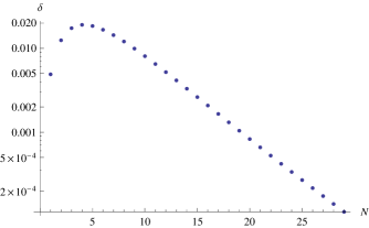
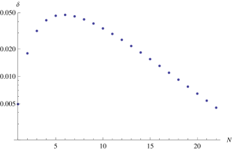
$N_{f}=7$	$N_{f}=9$
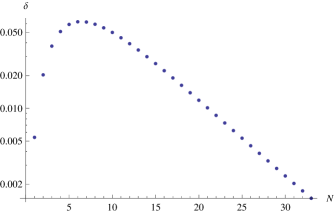
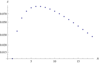
$N_{f}=10$	$N_{f}=11$
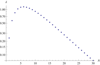
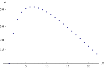
$N_{f}=14$	$N_{f}=16$

Figure 4: We plot $\delta$ defined in (3.28) for $N_{f}=7,9,10,11,14,16$. Note that the vertical axis is log scale. One can see that $\delta$ is indeed exponentially suppressed as $N$ grows.

As a further test, we consider the large $N_{f}$ limit of (3.24) with $\widehat{\mu}=\mu/N_{f}$ fixed. It is not difficult to see

$$f_{0,1}(N_{f},\mu) =\frac{N_{f}^{2}}{\pi^{2}}\left(-\widehat{\mu}-\frac{1}{4}\right)-\frac{2}{3}\widehat{\mu}-\frac{1}{6}+\mathcal{O}(N_{f}^{-2}),$$ (3.29)

$$f_{0,2}(N_{f},\mu) =\frac{N_{f}^{2}}{\pi^{2}}\left(-4\widehat{\mu}^{2}+\frac{1}{4}\widehat{\mu}-\frac{7}{32}\right)-6\widehat{\mu}+\frac{11}{12}+\mathcal{O}(N_{f}^{-2}),$$

$$f_{0,3}(N_{f},\mu) =\frac{N_{f}^{2}}{\pi^{2}}\left(-\frac{128}{3}\widehat{\mu}^{3}+16\widehat{\mu}^{2}-\frac{46}{9}\widehat{\mu}+\frac{11}{27}\right)$$

$$\quad+\frac{1792\widehat{\mu}^{3}}{9}-\frac{992\widehat{\mu}^{2}}{3}+\frac{356\widehat{\mu}}{3}-\frac{134}{9}+\mathcal{O}(N_{f}^{-2}).$$

The leading terms exactly coincide with the genus zero contribution of the grand potential in the ’t Hooft limit computed in appendix C. We stress that our conjecture (3.24) gives an all-genus prediction in the ’t Hooft expansion. It would be very interesting to confirm whether our conjecture indeed reproduces the higher genus corrections.

From (3.24), we expect that the worldsheet $m$-instanton coefficient $f_{0,m}(N_{f},\mu)$ has the following general structure:

• $f_{0,m}$ is an $m^{\textrm{th}}$ order polynomial of $\mu$, and the highest order term is $P_{1}^{m}$.

• Most of the terms of $f_{0,m}$ have the same “degree” $m$, i.e. they have the form of $\prod_{l}P_{l}^{k_{l}}$ with $\sum lk_{l}=m$, but some remaining terms have smaller degree $\sum lk_{l}<m$.

• The coefficient of each term in $f_{0,m}$ is a combination of $s_{n}~{}(n\leq 2m)$.

It would be interesting to understand the origin of this structure and the general rule to find the coefficients.

4 Membrane instanton corrections

In the previous section, we extracted the non-perturbative corrections to the grand potential from the exact values of the partition function for some integral values of $N_{f}$. Based on these results, we proposed the analytic forms of the worldsheet instanton corrections up to $m=3$. As mentioned before, the grand potential also receives the non-perturbative corrections from the membrane instantons. In this section, we explore analytic forms of these corrections. The membrane instanton correction corresponds to $m=0$ in (3.10),

$$J^{\text{M2}}(N_{f},\mu)=\sum_{\ell=1}^{\infty}f_{\ell,0}(N_{f},\mu)e^{-2\ell\mu}.$$ (4.1)

We want to determine the coefficient $f_{\ell,0}(N_{f},\mu)$. Unfortunately, we do not have a systematic way to compute $f_{\ell,0}(N_{f},\mu)$. Here, we try to fix it from many constraints. The same idea was originally used in the ABJM Fermi-gas HMO2 . We first investigate the expansion of the grand potential around $N_{f}=0$. We then consider the singularity structure of $f_{\ell,0}(N_{f},\mu)$. Using these constraints, we present exact forms of $f_{1,0}(N_{f},\mu)$ and a part of $f_{2,0}(N_{f},\mu)$. To fix the higher instanton corrections, we need more information.

4.1 Semi-classical analysis from TBA

We here study the expansion of the grand potential $J(N_{f},z)$ around $N_{f}=0$. Let us consider what kind of corrections the grand potential receives in the semi-classical limit $N_{f}\to 0$. We first observe that $Z_{1}=\operatorname{Tr}\rho$ can be computed exactly GM ,

$$Z_{1}=\frac{1}{4\pi}\int_{-\infty}^{\infty}\frac{dx}{(2\cosh\frac{x}{2})^{N_{f}}}=\frac{1}{4\pi}\frac{\Gamma^{2}(N_{f}/2)}{\Gamma(N_{f})}.$$ (4.2)

This has the following semi-classical expansion

$$Z_{1}=\frac{1}{\pi N_{f}}-\frac{\pi N_{f}}{24}+\frac{\zeta(3)}{4\pi}N_{f}^{2}-\frac{\pi^{3}}{640}N_{f}^{3}+\left(-\frac{\pi\zeta(3)}{96}+\frac{3\zeta(5)}{16\pi}\right)N_{f}^{4}+\mathcal{O}(N_{f}^{5}).$$ (4.3)

This observation suggests that the grand potential also has the similar semi-classical expansion

$$J(N_{f},z)=\frac{1}{N_{f}}J_{0}(z)+N_{f}J_{1}(z)+N_{f}^{2}J_{3/2}(z)+N_{f}^{3}J_{2}(z)+N_{f}^{4}J_{5/2}(z)+\mathcal{O}(N_{f}^{5}),$$ (4.4)

because $J(N_{f},z)$ is a kind of generating function of $Z_{n}=\operatorname{Tr}\rho^{n}$. The absence of the constant $\mathcal{O}(N_{f}^{0})$ contribution is not obvious only from this observation, but the TBA analysis below supports this. The leading contribution $J_{0}(z)$ has already been computed in GM . Note that in the ABJM Fermi-gas, the even power terms $k^{2n}$ do not appear in the semi-classical expansion. This is a big difference between the $N_{f}$ matrix model and the ABJM case. Here we compute $J_{1}(z)$ from the TBA equations.

What we should do is to solve the functional relations (2.13) and (2.14) in the semi-classical limit $N_{f}\to 0$ as in CM . To do so, we rescale all the functions by

$$\widehat{R}_{\pm}(x)=R_{\pm}\left(\frac{x}{N_{f}}\right),\quad\widehat{\eta}(x)=\eta\left(\frac{x}{N_{f}}\right),\quad\widehat{U}(x)=U\left(\frac{x}{N_{f}}\right),$$ (4.5)

Then the equations (2.13) and (2.14) become

$$\widehat{R}_{+}\left(x+\frac{\pi iN_{f}}{2}\right)\widehat{R}_{+}\left(x-\frac{\pi iN_{f}}{2}\right)\exp\left[\widehat{U}\left(x+\frac{\pi iN_{f}}{2}\right)+\widehat{U}\left(x-\frac{\pi iN_{f}}{2}\right)\right] =1+\widehat{\eta}^{2}(x),$$ (4.6)

$$\widehat{\eta}\left(x+\frac{\pi iN_{f}}{2}\right)+\widehat{\eta}\left(x-\frac{\pi iN_{f}}{2}\right) =-z\widehat{R}_{+}(x),$$

and

$$\frac{\widehat{R}_{-}(x+\frac{\pi iN_{f}}{2})}{\widehat{R}_{+}(x+\frac{\pi iN_{f}}{2})}-\frac{\widehat{R}_{-}(x-\frac{\pi iN_{f}}{2})}{\widehat{R}_{+}(x-\frac{\pi iN_{f}}{2})}=2iN_{f}\frac{\widehat{\eta}^{\prime}(x)}{1+\widehat{\eta}^{2}(x)}.$$ (4.7)

These are formally the same forms as the ones in (4.10) and (4.11) of CM with $k=N_{f}$. The only but big difference is the explicit form of the potential $\widehat{U}(x)$.

We assume that the functional equations (4.6) and (4.7) admit the semi-classical expansions around $N_{f}=0$. The important point is that the potential part in (4.6) has the following “semi-classical” expansion

$$\widehat{U}\left(x+\frac{\pi iN_{f}}{2}\right)+\widehat{U}\left(x-\frac{\pi iN_{f}}{2}\right)=|x|+N_{f}\log(1+e^{-\frac{2|x|}{N_{f}}})\qquad(N_{f}\to 0).$$ (4.8)

The second term on the right hand side in (4.8) looks like a “non-perturbative” term in $N_{f}$. However, the integration of $e^{-2|x|/N_{f}}$ may potentially cause the perturbative corrections, for example,

$$\int_{-\infty}^{\infty}dx\,e^{-\frac{2|x|}{N_{f}}}=N_{f}.$$ (4.9)

Therefore we cannot drop the second term even in the semi-classical analysis. As in CM , we formally solve (4.6) and (4.7) by the semi-classical expansions,

$$r(x) =\widehat{R}_{+}(x)=\sum_{n=0}^{\infty}r_{n}(x)N_{f}^{n},\qquad\widehat{\eta}(x)=\sum_{n=0}^{\infty}\eta_{n}(x)N_{f}^{n},$$ (4.10)

$$t(x) =\frac{\widehat{R}_{-}(x)}{\widehat{R}_{+}(x)}=\sum_{n=0}^{\infty}t_{n}(x)N_{f}^{n}.$$

This can be done systematically up to any desired order in principle. In appendix B, we give explicit forms up to $n=3$.

Once the solutions of (4.6) and (4.7) are found, we can compute the grand potential from (2.12). Let us define

$$I_{\pm,n}\equiv\int_{0}^{\infty}\frac{dx}{2\pi}\widehat{R}_{\pm,n}(x),\qquad\widehat{R}_{\pm}(x)=\sum_{n=0}^{\infty}N_{f}^{n}\widehat{R}_{\pm,n}(x),$$ (4.11)

where $\widehat{R}_{\pm,n}(x)$ are related to $r_{n}(x)$ and $t_{n}(x)$ in (4.10). Using the solutions in appendix B, one can check that $I_{\pm,n}$ up to $n=3$ has the following expansions around $N_{f}=0$:

$$I_{+,0} =\frac{2}{\pi z}\arcsin\left(\frac{z}{2}\right),\qquad I_{-,0}=-\frac{2}{\pi^{2}z}\arcsin^{2}\left(\frac{z}{2}\right),$$ (4.12)

$$I_{\pm,1} =N_{f}I_{\pm,1}^{(1)}+N_{f}^{2}I_{\pm,1}^{(2)}+\mathcal{O}(N_{f}^{3}),$$

$$I_{\pm,2} =I_{\pm,2}^{(0)}+N_{f}I_{\pm,2}^{(1)}+\mathcal{O}(N_{f}^{2}),$$

$$I_{\pm,3} =N_{f}^{-1}I_{\pm,3}^{(-1)}+I_{\pm,3}^{(0)}+\mathcal{O}(N_{f}),$$

The explicit forms of these coefficients are also listed in appendix B. We also observe that the higher order corrections have the following expansions:

$$I_{\pm,2n} =N_{f}^{-2n+3}I_{\pm,2n}^{(-2n+3)}+\mathcal{O}(N_{f}^{-2n+4})\quad(n=2,3,\cdots),$$ (4.13)

$$I_{\pm,2n+1} =N_{f}^{-2n+2}I_{\pm,2n+1}^{(-2n+2)}+\mathcal{O}(N_{f}^{-2n+3})\quad(n=2,3,\cdots).$$

Combining all the above results, the grand potential is given by

$$J_{z}^{\pm}(z) =\frac{1}{2\pi N_{f}}\int_{0}^{\infty}dx\,\widehat{R}_{\pm}(x)=\frac{1}{N_{f}}\sum_{n=0}^{\infty}N_{f}^{n}I_{\pm,n}$$ (4.14)

$$=\frac{I_{\pm,0}}{N_{f}}+N_{f}(I_{\pm,1}^{(1)}+I_{\pm,2}^{(0)}+I_{\pm,3}^{(-1)})+N_{f}^{2}(I_{\pm,1}^{(2)}+I_{\pm,2}^{(1)}+I_{\pm,3}^{(0)}+\cdots)+\mathcal{O}(N_{f}^{3}).$$

where $J_{z}^{\pm}(z)=\partial J^{\pm}(z)/\partial z$.

The leading term is given by

$$J_{0,z}^{+}(z)=\frac{2}{\pi z}\arcsin\left(\frac{z}{2}\right),\qquad J_{0,z}^{-}(z)=-\frac{2}{\pi^{2}z}\arcsin^{2}\left(\frac{z}{2}\right).$$ (4.15)

This result indeed agrees with (3.73) in GM . The next-to-leading term is also given by

$$J_{1,z}^{+}(z) =-\frac{\pi(16-z^{2})}{12(4-z^{2})^{5/2}},$$ (4.16)

$$J_{1,z}^{-}(z) =\frac{z(8-z^{2})}{8(4-z^{2})^{2}}+\frac{16-z^{2}}{6(4-z^{2})^{5/2}}\arctan\left(\frac{z}{\sqrt{4-z^{2}}}\right),$$

After integrating over $z$, we finally obtain

$$J_{1}(z)=\frac{z^{2}}{24(4-z^{2})}-\frac{z(16-3z^{2})}{48(4-z^{2})^{3/2}}\left[\pi-2\arctan\left(\frac{z}{\sqrt{4-z^{2}}}\right)\right],$$ (4.17)

where we have fixed the integration constant such that $J_{1}(0)=0$. Note that $J_{1}^{+}(z)$ and $J_{1}^{-}(z)$ have branch cuts for $|z|>2$. However, the branch cut along $z>2$ disappears in the total potential $J_{1}(z)$, and there is no discontinuity in $J_{1}(z)$ along the positive real axis in the $z$-plane. In the large $z$ (or $\mu$) limit, $J_{0}(z)$ and $J_{1}(z)$ behave as

$$J_{0}(z) =\frac{2\mu^{3}}{3\pi^{2}}+\frac{\mu}{2}+\frac{\zeta(3)}{\pi^{2}}+\frac{2\mu+1}{\pi^{2}}e^{-2\mu}+\frac{12\mu-1}{8\pi^{2}}e^{-4\mu}+\mathcal{O}(\mu e^{-6\mu}),$$ (4.18)

$$J_{1}(z) =-\frac{\mu}{8}-\frac{1}{24}-\frac{2\mu+1}{24}e^{-2\mu}+\frac{12\mu-19}{48}e^{-4\mu}+\mathcal{O}(\mu e^{-6\mu}).$$

The cubic and linear terms in $\mu$ are consistent with the large $\mu$ behavior in (3.8). The constant terms also match the expansion of $A(N_{f})$ in (3.16). The exponentially suppressed terms will be used to fix the membrane instanton correction $f_{\ell,0}(N_{f},\mu)$.

Let us remark on the higher order corrections. The next-to-next-to-leading correction is given by

$$J_{3/2,z}^{\pm}(z)=I_{\pm,1}^{(2)}+I_{\pm,2}^{(1)}+I_{\pm,3}^{(0)}+\cdots=\sum_{n=1}^{\infty}I_{\pm,n}^{(-n+3)}.$$ (4.19)

Thus to compute $J_{3/2}(z)$, we need the infinite series of corrections $I_{\pm,n}^{(-n+3)}$ ($n\geq 1$). This means that it is very difficult to compute the semi-classical expansion beyond this order in this approach. We need a more efficient way to resolve this problem.

One possible way is to expand the density matrix around $N_{f}=0$ from the beginning. Let us see it briefly. We use the identity

$$\frac{1}{(2\cosh\frac{x}{2N_{f}})^{N_{f}/2}}=\exp\left[-\frac{N_{f}}{2}\log\left(2\cosh\frac{x}{2N_{f}}\right)\right]=e^{-\frac{|x|}{4}}\sum_{k=0}^{\infty}\frac{N_{f}^{k}}{k!}\ell^{k}(x),$$ (4.20)

where

$$\ell(x)=-\frac{1}{2}\log(1+e^{-|x|/N_{f}}).$$ (4.21)

We consider the rescaled density matrix

$$\widetilde{\rho}(x_{1},x_{2}) =\frac{1}{N_{f}}\rho\left(\frac{x_{1}}{N_{f}},\frac{x_{2}}{N_{f}}\right)$$ (4.22)

$$=\frac{1}{2\pi N_{f}}\frac{1}{(2\cosh\frac{x_{1}}{2N_{f}})^{N_{f}/2}}\frac{1}{(2\cosh\frac{x_{2}}{2N_{f}})^{N_{f}/2}}\frac{1}{2\cosh(\frac{x_{1}-x_{2}}{2N_{f}})}.$$

It is easy to check the equality $\operatorname{Tr}\widetilde{\rho}^{n}=\operatorname{Tr}\rho^{n}$. Then, the density matrix is expanded as

$$\widetilde{\rho}(x_{1},x_{2}) =\frac{1}{2\pi N_{f}}\frac{e^{-\frac{|x_{1}|}{4}-\frac{|x_{2}|}{4}}}{2\cosh(\frac{x_{1}-x_{2}}{2N_{f}})}\sum_{k=0}^{\infty}\frac{N_{f}^{k}}{k!}(\ell(x_{1})+\ell(x_{2}))^{k}$$ (4.23)

$$=\rho_{0}(x_{1},x_{2})+N_{f}\rho_{1}(x_{1},x_{2})+N_{f}^{2}\rho_{2}(x_{1},x_{2})+\cdots,$$

where

$$\rho_{0}(x_{1},x_{2})=\frac{1}{2\pi N_{f}}\frac{e^{-\frac{|x_{1}|}{4}-\frac{|x_{2}|}{4}}}{2\cosh(\frac{x_{1}-x_{2}}{2N_{f}})},\qquad\rho_{k}(x_{1},x_{2})=\frac{1}{k!}\rho_{0}(x_{1},x_{2})(\ell(x_{1})+\ell(x_{2}))^{k}.$$ (4.24)

The trace of $\widetilde{\rho}$ can be computed as follows:

$$Z_{n} =\operatorname{Tr}\widetilde{\rho}^{n}=\operatorname{Tr}[(\rho_{0}+N_{f}\rho_{1}+N_{f}^{2}\rho_{2}^{2}+\cdots)^{n}]$$ (4.25)

$$=\operatorname{Tr}\rho_{0}^{n}+nN_{f}\operatorname{Tr}\rho_{0}^{n-1}\rho_{1}+nN_{f}^{2}\operatorname{Tr}\rho_{0}^{n-1}\rho_{2}$$

$$\quad+N_{f}^{2}[\operatorname{Tr}\rho_{0}^{n-2}\rho_{1}^{2}+(\text{permutations})]+\mathcal{O}(N_{f}^{3}).$$

Thus we find

$$J(N_{f},z) =-\sum_{n=1}^{\infty}\frac{(-z)^{n}}{n}Z_{n}=-\sum_{n=1}^{\infty}\frac{(-z)^{n}}{n}[\operatorname{Tr}\rho_{0}^{n}+nN_{f}\operatorname{Tr}\rho_{0}^{n-1}\rho_{1}+\cdots]$$ (4.26)

$$=J_{\text{ud}}(N_{f},z)-N_{f}\sum_{n=1}^{\infty}(-z)^{n}\operatorname{Tr}\rho_{0}^{n-1}\rho_{1}+\cdots$$

where $J_{\text{ud}}(N_{f},z)$ is the grand potential for the undeformed kernel $\rho_{0}$. The second term is rewritten as

$$\sum_{n=1}^{\infty}(-z)^{n}\operatorname{Tr}\rho_{0}^{n-1}\rho_{1} =2\sum_{n=1}^{\infty}(-z)^{n}\int_{-\infty}^{\infty}dx_{1}\int_{-\infty}^{\infty}dx_{2}\,\rho_{0}^{n-1}(x_{1},x_{2})\rho_{0}(x_{2},x_{1})\ell(x_{1})$$ (4.27)

$$=2\sum_{n=1}^{\infty}(-z)^{n}\int_{-\infty}^{\infty}dx\,\rho_{0}^{n}(x,x)\ell(x)$$

$$=-2\int_{-\infty}^{\infty}dx\frac{z\rho_{0}}{1+z\rho_{0}}(x,x)\ell(x).$$

The semi-classical expansion of $\rho_{0}^{n}(x,x)$ can be computed from the TBA for $\rho_{0}(x)$.

An advantage of this approach is that the undeformed kernel $\rho_{0}$ does not contain the “non-perturbative” term in (4.8). It is interesting to consider whether this approach resolves the difficulty of the computation of $J_{3/2}(z)$.

4.2 Pole cancellation mechanism

The worldsheet instanton correction conjectured in section 3 has singularities for some (in particular, integral) values of $N_{f}$. These singularities must be canceled by the other contributions because the partition function itself is always finite. This pole cancellation mechanism was first found in the ABJM theory HMO2 . As emphasized in CM , this mechanism is conceptually important because it implies that the ’t Hooft expansion breaks down at some finite values of the string coupling $g_{s}$. One needs to consider a non-perturbative completion to cure the divergences. Our conjecture (3.24) shows that this mechanism also exists in the $N_{f}$ matrix model.

A technical merit of this mechanism is that we can know the pole structure of the membrane instanton correction from that of the worldsheet instanton correction. As an example, let us consider the order $\mathcal{O}(e^{-2\mu})$ correction for $N_{f}=2$. Looking at (3.10), there are two contributions at this order. One is the worldsheet one-instanton correction $f_{0,1}$, and the other is the membrane one-instanton correction $f_{1,0}$. It is easy to see that the worldsheet one-instanton correction in (3.24) has the following singularity at $N_{f}=2$.

$$\lim_{N_{f}\to 2}f_{0,1}(N_{f},\mu)e^{-\frac{4\mu}{N_{f}}}=-\frac{2(2\mu+1)}{\pi^{2}(N_{f}-2)}e^{-2\mu}-\frac{2(2\mu^{2}+2\mu+1)}{\pi^{2}}e^{-2\mu}+\mathcal{O}(N_{f}-2).$$ (4.28)

This singularity must be canceled by the membrane one-instanton correction. This means that $f_{1,0}$ must behave as

$$\lim_{N_{f}\to 2}f_{1,0}(N_{f},\mu)=\frac{2(2\mu+1)}{\pi^{2}(N_{f}-2)}+\mathcal{O}(1).$$ (4.29)

Similarly, the singularities of $f_{1,0}$ at $N_{f}=4$ and $N_{f}=6$ are determined by the $f_{0,2}$ and $f_{0,3}$, respectively. It is easy to find

$$\lim_{N_{f}\to 4}f_{1,0}(N_{f},\mu) =\frac{6(2\mu+1)}{\pi^{2}(N_{f}-4)}+\mathcal{O}(1),$$ (4.30)

$$\lim_{N_{f}\to 6}f_{1,0}(N_{f},\mu) =\frac{20(2\mu+1)}{\pi^{2}(N_{f}-6)}+\mathcal{O}(1).$$

We will use these results to fix $f_{1,0}(N_{f},\mu)$.

4.3 Fixing the leading membrane instanton correction

Now we are in position to conjecture an exact form of $f_{1,0}(N_{f},\mu)$. The large $\mu$ expansion of the semi-classical results $J_{0}(z)$ and $J_{1}(z)$ suggests that the membrane $\ell$-instanton coefficient $f_{\ell,0}$ is a linear function of $\mu$ for all $\ell$

$$f_{\ell,0}(N_{f},\mu)=a_{\ell}(N_{f})\mu+b_{\ell}(N_{f}).$$ (4.31)

To fix $f_{1,0}(N_{f},\mu)$, we use the following three constraints:

• The singularity structure at $N_{f}=2,4,6$ is given by (4.29) and (4.30).

• As noted in subsection 3.4, $f_{1,0}(N_{f},\mu)$ must vanish for odd $N_{f}$.

• The semi-classical expansion of $f_{1,0}(N_{f},\mu)$ is given by

  $$f_{1,0}(N_{f},\mu)=\frac{2\mu+1}{\pi^{2}N_{f}}-\frac{2\mu+1}{24}N_{f}+\mathcal{O}(N_{f}^{2})\qquad(N_{f}\to 0).$$ (4.32)

The results (4.29), (4.30) and (4.32) strongly suggest that $f_{1,0}(N_{f},\mu)$ has the following universal form for any $N_{f}$,

$$f_{1,0}(N_{f},\mu)=b_{1}(N_{f})(2\mu+1),\qquad a_{1}(N_{f})=2b_{1}(N_{f}).$$ (4.33)

We can check that this is indeed the case. In figure 5(a), we show the ratio $a_{1}(N_{f})/b_{1}(N_{f})$ computed numerically from the TBA equations (2.10) and (2.11) for $N_{f}=3/20,4/20,\dots,19/20$. The ratio does not depend on $N_{f}$, and is very close to $2$.

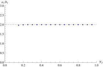
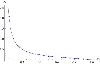
(a)	(b)

Figure 5: (a) We plot the ratio $a_{1}(N_{f})/b_{1}(N_{f})$ in (4.33) against $N_{f}$. These values are estimated by using the TBA equations (2.10) and (2.11). The ratio does not depend on $N_{f}$. (b) We compare the analytic conjecture (4.34) with the numerically estimated values from TBA.

Combining all the above results, we arrive at a conjecture of $b_{1}(N_{f})$,

$$b_{1}(N_{f})=-\frac{\Gamma^{2}(-N_{f}/2)}{4\pi^{2}\Gamma(-N_{f})}.$$ (4.34)

The small $N_{f}$ expansion reads

$$b_{1}(N_{f})=\frac{1}{\pi^{2}N_{f}}-\frac{N_{f}}{24}-\frac{\zeta(3)N_{f}^{2}}{4\pi^{2}}-\frac{\pi^{2}N_{f}^{3}}{640}+\left(\frac{\zeta(3)}{96}-\frac{3\zeta(5)}{16\pi^{2}}\right)N_{f}^{4}+\mathcal{O}(N_{f}^{5}).$$ (4.35)

Of course, this reproduces (4.32). One non-trivial check of the conjecture (4.34) is to compute the finite parts for $N_{f}=2,4,6$. For example, in the limit $N_{f}\to 2$, one finds

$$\lim_{N_{f}\to 2}(f_{1,0}(N_{f},\mu)e^{-2\mu}+f_{0,1}(N_{f},\mu)e^{-\frac{4\mu}{N_{f}}})=-\frac{4\mu^{2}+2\mu+1}{\pi^{2}}e^{-2\mu}.$$ (4.36)

This result indeed reproduces the correct coefficient of $e^{-2\mu}$ in (B.2). In this way, one can also check that the coefficients of $e^{-2\mu}$ in (B.4) and (B.5) are reproduced by the combinations $f_{1,0}e^{-2\mu}+f_{0,2}e^{-\frac{8\mu}{N_{f}}}$ ($N_{f}\to 4$) and $f_{1,0}e^{-2\mu}+f_{0,3}e^{-\frac{12\mu}{N_{f}}}$ ($N_{f}\to 6$), respectively. As another check, we compare the numerical values computed from TBA with our conjecture (4.34) for various values of $N_{f}$. The result is shown in figure 5(b). These tests present strong supports for our conjecture (4.34).

4.4 Remark on higher instanton corrections

Let us remark on the higher instanton corrections. So far, we do not know how to determine $a_{\ell}(N_{f})$ and $b_{\ell}(N_{f})$ systematically. Let us consider the next simplest case: $\ell=2$. From (4.18), these must have the small $N_{f}$ expansions,

$$a_{2}(N_{f})=\frac{3}{2\pi^{2}N_{f}}+\frac{1}{4}N_{f}+\mathcal{O}(N_{f}^{2}),\qquad b_{2}(N_{f})=-\frac{1}{8\pi^{2}N_{f}}-\frac{19}{48}N_{f}+\mathcal{O}(N_{f}^{2}).$$ (4.37)

Furthermore, $f_{2,0}(N_{f},\mu)$ must cancel the poles of $f_{0,1}(N_{f},\mu)$ at $N_{f}=1$ and $f_{0,3}(N_{f},\mu)$ at $N_{f}=3$. These conditions give the constraints

$$\lim_{N_{f}\to 1}a_{2}(N_{f}) =-\frac{1}{\pi^{2}(N_{f}-1)}+\mathcal{O}(1),\qquad\lim_{N_{f}\to 1}b_{2}(N_{f})=-\frac{1}{4\pi^{2}(N_{f}-1)}+\mathcal{O}(1),$$ (4.38)

$$\lim_{N_{f}\to 3}a_{2}(N_{f}) =-\frac{10}{\pi^{2}(N_{f}-3)}+\mathcal{O}(1),\qquad\lim_{N_{f}\to 3}b_{2}(N_{f})=-\frac{5}{2\pi^{2}(N_{f}-3)}+\mathcal{O}(1).$$

We find an analytic form of $a_{2}(N_{f})$ satisfying all these constraints

$$a_{2}(N_{f})=-\frac{1}{4\pi^{2}}\left(1+\frac{2}{\cos\pi N_{f}}\right)\frac{\Gamma^{2}(-N_{f})}{\Gamma(-2N_{f})}.$$ (4.39)

This guess correctly reproduces the finite parts for $N_{f}=1,3$ in appendix B. It also shows a good agreement with the numerical values from TBA as shown in figure 6(a).

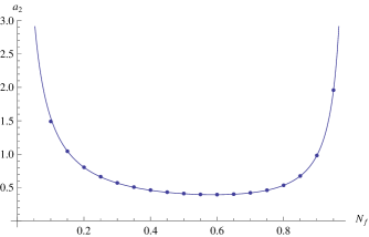
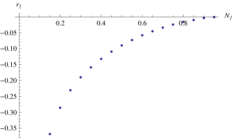
(a)	(b)

Figure 6: We plot (a) $a_{2}(N_{f})$ and (b) $r_{2}(N_{f})=b_{2}(N_{f})-a_{2}(N_{f})/4$ against $N_{f}$.

We also want to fix $b_{2}(N_{f})$. Unfortunately, the ratio $b_{2}(N_{f})/a_{2}(N_{f})$ is no longer a constant unlike the one-instanton correction. Instead, it is convenient to define a new function by

$$r_{\ell}(N_{f})=b_{\ell}(N_{f})-\frac{a_{\ell}(N_{f})}{2\ell}.$$ (4.40)

In other words, we parametrize the membrane $\ell$-instanton coefficient as

$$f_{\ell,0}(N_{f},\mu)=\Big{(}\mu+\frac{1}{2\ell}\Big{)}a_{\ell}(N_{f})+r_{\ell}(N_{f}).$$ (4.41)

For $\ell=1$, we found in (4.33) that the last term is absent: $r_{1}(N_{f})=0$. For $\ell\geq 2$, it turns out that $r_{\ell}(N_{f})$ is a non-trivial function of $N_{f}$. From the pole structure (4.38), one finds that the function $r_{2}(N_{f})$ is regular at $N_{f}=1,3$. Furthermore, in order to reproduce the finite parts for $N_{f}=1,3$ in (B.1) and (B.3) correctly, $r_{2}(N_{f})$ must vanish in the limit $N_{f}\to 1,3$:

$$\lim_{N_{f}\to 1}r_{2}(N_{f})=\lim_{N_{f}\to 3}r_{2}(N_{f})=0.$$ (4.42)

Also, $r_{2}(N_{f})$ must have the following semi-classical expansion

$$r_{2}(N_{f})=-\frac{1}{2\pi^{2}N_{f}}-\frac{11}{24}N_{f}+\mathcal{O}(N_{f}^{2})\qquad(N_{f}\to 0).$$ (4.43)

In figure 6(b), we plot $r_{2}(N_{f})$ for $0<N_{f}<1$ as a function of $N_{f}$. As expected, $r_{2}(N_{f})$ goes to zero as $N_{f}\to 1$. So far, we have not found an exact form of $r_{2}(N_{f})$. To fix it, we might need more information.

Interestingly, the combination $(\mu+\frac{1}{2n})a_{n}(N_{f})$ seems to cancel the poles of the worldsheet instantons when there are no bound state contributions. For example, for $N_{f}=2/n$ ($n=1,2,3,\dots$), the worldsheet 1-instanton correction has the following pole structure:

$$\lim_{N_{f}\to 2/n}f_{0,1}(N_{f},\mu)e^{-\frac{4\mu}{N_{f}}}=(-1)^{n}\frac{4(\mu+\frac{1}{2n})}{n^{2}\pi^{2}(N_{f}-\frac{2}{n})}e^{-2n\mu}+\mathcal{O}(1).$$ (4.44)

This pole must be canceled by the membrane $n$-instanton correction because there are no bound state contributions at this order. Thus, focusing on the $\mu e^{-2n\mu}$ term, one finds that $a_{n}(N_{f})$ must behave at $N_{f}=2/n$ as

$$\lim_{N_{f}\to 2/n}a_{n}(N_{f})=(-1)^{n-1}\frac{4}{n^{2}\pi^{2}(N_{f}-\frac{2}{n})}+\mathcal{O}(1),$$ (4.45)

and that the combination $(\mu+\frac{1}{2n})a_{n}(N_{f})$ indeed cancels the pole in (4.44). Therefore we conclude that $r_{n}(N_{f})$ is regular at $N_{f}=2/n$:

$$\lim_{N_{f}\to 2/n}r_{n}(N_{f})=\mathcal{O}(1).$$ (4.46)

It would be interesting to clarify the analytic structure of $r_{n}(N_{f})$ in more detail.

5 Conclusions

In this paper we have studied the large $N$ non-perturbative effects in the $N_{f}$ matrix model. Combining the exact computation of the partition function and the analysis of TBA, we have successfully determined a first few terms of both the worldsheet instanton corrections and the membrane instanton corrections, as analytic functions of $N_{f}$. These analytic results show that the pole cancellation mechanism, originally found in the ABJM model HMO2 , works also for the $N_{f}$ matrix model. As emphasized in GM , this clearly shows that the ’t Hooft expansion alone is incomplete and the existence of both membrane instantons and worldsheet instantons is necessary for the non-perturbative definition of the theory and the free energy to be finite at the physical value of the coupling. We would like to emphasize that this mechanism is invisible as long as one focuses on the small/large $N_{f}$ limit. One needs to consider the M-theory (or finite coupling) regime to see it. It is desirable to check that this mechanism works more generally, by computing the higher instanton coefficients of worldsheet instantons, membrane instantons, and their bound states. It is also interesting to apply the Fermi-gas approach to BPS Wilson loops along the lines of Klemm:2012ii ; Hatsuda:2013yua ; Hirano:2014bia . Moreover, it would be interesting to explore the non-perturbative structure for other examples Mezei:2013gqa ; Anderson:2014hxa .

To proceed further, we need to develop a systematic way to study this model. In particular, it is very interesting to find an efficient method to compute the small $N_{f}$ expansion of the grand potential, which gives important clues to determine the analytic form of the membrane instantons. As for the worldsheet instantons, using the technique of ordinary matrix models we can in principle compute the genus expansion in the ’t Hooft limit, order by order in $1/N_{f}$. However, to discuss the pole cancellation, we need to resum this series à la Gopakumar-Vafa, which is a formidable task. Also, currently we do not have enough information to study the effect of bound states of worldsheet instantons and membrane instantons. We leave them as interesting future problems.

We found that the structure of the instanton corrections in the $N_{f}$ matrix model is quite different from that of the ABJM model. In the ABJM case, the membrane instanton correction and the worldsheet instanton correction have the following form MP2 ; HMO2

$$J^{\text{M2}}_{\text{ABJM}}(k,\mu) =\sum_{\ell=1}^{\infty}(a_{\ell}(k)\mu^{2}+b_{\ell}(k)\mu+c_{\ell}(k))e^{-2\ell\mu},$$ (5.1)

$$J^{\text{WS}}_{\text{ABJM}}(k,\mu) =\sum_{m=1}^{\infty}d_{m}(k)e^{-\frac{4m\mu}{k}},$$

where all the coefficients $a_{\ell}(k)$, $b_{\ell}(k)$, $c_{\ell}(k)$ and $d_{m}(k)$ are expressed in terms of a combination of the trigonometric functions. On the other hand, in the case of $N_{f}$ matrix model, we conjecture that the membrane instanton correction and the worldsheet instanton correction have the following structure

$$J^{\text{M2}}(N_{f},\mu) =\sum_{\ell=1}^{\infty}(a_{\ell}(N_{f})\mu+b_{\ell}(N_{f}))e^{-2\ell\mu},$$ (5.2)

$$J^{\text{WS}}(N_{f},\mu) =\sum_{m=1}^{\infty}\Big{(}\sum_{\sum lk_{l}\leq m}d_{m}^{(k_{1},\cdots,k_{m})}(N_{f})\prod_{l=1}^{m}P_{l}^{k_{l}}(N_{f},\mu)\Big{)}e^{-\frac{4m\mu}{N_{f}}},$$

where $P_{l}(N_{f},\mu)$ is defined in (3.23). We found that the membrane instanton coefficients in (4.34) and (4.39) are expressed in terms of the gamma function (and the trigonometric functions). As another difference, the pre-factor of the worldsheet instanton correction depends on $\mu$, unlike the ABJM case. More precisely, the worldsheet $m$-instanton coefficient is given by an $m^{\text{th}}$ order polynomial of $\mu$, and the coefficient $d_{m}^{(k_{1},\cdots,k_{m})}(N_{f})$ appearing in (5.2) is a combination of the trigonometric functions (3.24). This difference between the $N_{f}$ matrix model and the ABJM model may be related to the difference of the orbifolding on the bulk side: the orbifold $\mathbb{C}^{2}\times\mathbb{C}^{2}/\mathbb{Z}_{N_{f}}$, corresponding to the $N_{f}$ matrix model, has a family of $A_{N_{f}-1}$ ALE singularity parametrized by the first factor $\mathbb{C}^{2}$, while the singularity of $\mathbb{C}^{4}/\mathbb{Z}_{k}$ for the ABJM case is isolated. Perhaps, the structure of the worldsheet instantons in the $N_{f}$ matrix model might be understood as the effect of a non-isolated family of rational curves (see Beasley:2005iu for such worldsheet instanton effects in a heterotic string compactification).

The spectral problem in the Fermi-gas is also important. The spectrum of the one-dimensional Fermi-gas that we are considering is determined by the Fredholm integral equation of the first kind MP2 :

$$\int_{-\infty}^{\infty}dx^{\prime}\rho(x,x^{\prime})\phi(x^{\prime})=e^{-E}\phi(x).$$ (5.3)

Since the density matrix $\rho(x_{1},x_{2})$ is a non-negative Hilbert-Schmidt operator, the integral equation (5.3) has a positive discrete spectrum. In the ABJ(M) Fermi-gas, the spectrum is determined by the exact WKB quantization condition KM ; Kallen:2014lsa (see also Huang:2014eha ), in which one has to consider not only the perturbative contribution but also the non-perturbative contribution in the Planck constant $\hbar=2\pi k$ to reproduce the correct spectrum. Since all the information of the (grand) partition function is encoded in the Fermi-gas spectrum, it is important to find the exact WKB quantization condition in the $N_{f}$ matrix model.

In the case of ABJ(M) model, we have a very detailed understanding of the instanton corrections thanks to the relation to the refined topological string on local $\mathbb{P}^{1}\times\mathbb{P}^{1}$ HMMO ; MM ; HO ; KM ; Kallen:2014lsa . This relation to the topological string is widely viewed as an accident of the ABJ(M) model. However, in view of the non-trivial relation (3.12) between the constant term $A(N_{f})$ of the $N_{f}$ matrix model and the constant map contribution $A_{\rm const}(k)$ of the topological string, it is tempting to speculate that the $N_{f}$ matrix model also has a hidden connection to the topological string on some background. It would be interesting to see if such a hidden connection to the topological string really exists, or not.

Finally, in this paper, we have probed the non-perturbative effects in M-theory from its gauge theory dual. Recently, there are some interesting progress on the gravity side Bhattacharyya:2012ye ; Dabholkar:2014wpa . It would be very significant to confirm our pole cancellation mechanism directly in M-theory in the future.

Appendix A A simpler expression of the constant map

In this appendix, we derive the integral expression (3.13) of the constant map $A_{\text{const}}(k)$ in the ABJM Fermi-gas (or equivalently in the topological string on local $\mathbb{P}^{1}\times\mathbb{P}^{1}$). A similar integral expression was found in KEK , but our expression is much simpler than theirs. Our starting point is the all-order small $k$ expansion found in KEK ,

$$A_{\text{const}}(k)=\frac{2\zeta(3)}{\pi^{2}k}+\sum_{n=1}^{\infty}\frac{(-1)^{n}}{(2n)!}B_{2n}B_{2n-2}\pi^{2n-2}k^{2n-1}.$$ (A.1)

To rewrite this as an integral form, we use the identity for the Bernoulli number:

$$B_{2n}=(-1)^{n-1}4n\int_{0}^{\infty}dx\frac{x^{2n-1}}{e^{2\pi x}-1}\quad(n\geq 1).$$ (A.2)

This identity is simply obtained from the integral expression of $\zeta(z)$ by setting $z=2n$. Then, we get

$$\sum_{n=1}^{\infty}\frac{(-1)^{n}}{(2n)!}B_{2n}B_{2n-2}\pi^{2n-2}k^{2n-1}=-\frac{2}{\pi}\int_{0}^{\infty}dx\frac{1}{e^{2\pi x}-1}\sum_{n=1}^{\infty}\frac{B_{2n-2}}{(2n-1)!}(\pi kx)^{2n-1}.$$ (A.3)

The sum can be performed,

$$\sum_{n=1}^{\infty}\frac{B_{2n-2}}{(2n-1)!}z^{2n-1}=\frac{z^{2}}{4}+\operatorname{Li}_{2}(1-e^{-z}).$$ (A.4)

Therefore we obtain the integral form

$$A_{\text{const}}(k)=\frac{2\zeta(3)}{\pi^{2}k}\left(1-\frac{k^{3}}{16}\right)-\frac{2}{\pi}\int_{0}^{\infty}dx\frac{\operatorname{Li}_{2}(1-e^{-\pi kx})}{e^{2\pi x}-1}.$$ (A.5)

After integration by parts, we finally get (3.13).

Appendix B Some explicit results

B.1 Corrections for integral $N_{f}$

Here we summarize the explicit forms of $J_{\text{np}}(N_{f},\mu)$ for $N_{f}=1,2,3,4,6,8,12$. For $N_{f}=1$, the partition function is equivalent to the one in the ABJM theory at $k=1$. We can use the result in HMO3 ,

$$J_{\text{np}}(1,\mu) =\biggl{[}\frac{4\mu^{2}+\mu+1/4}{\pi^{2}}\biggr{]}e^{-4\mu}+\biggl{[}-\frac{52\mu^{2}+\mu/2+9/16}{2\pi^{2}}+2\biggr{]}e^{-8\mu}$$

$$\quad+\biggl{[}\frac{736\mu^{2}-152\mu/3+77/18}{3\pi^{2}}-32\biggr{]}e^{-12\mu}$$

$$\quad+\biggl{[}-\frac{2701\mu^{2}-13949\mu/48+11291/768}{\pi^{2}}+466\biggr{]}e^{-16\mu}$$ (B.1)

$$\quad+\biggl{[}\frac{161824\mu^{2}-317122\mu/15+285253/300}{5\pi^{2}}-6720\biggr{]}e^{-20\mu}$$

$$\quad+\biggl{[}-\frac{1227440\mu^{2}-2686522\mu/15+631257/80}{3\pi^{2}}+\frac{292064}{3}\biggr{]}e^{-24\mu}+\mathcal{O}(e^{-28\mu}).$$

Similarly, in the case of $N_{f}=2$, we can use the ABJ result in MM ,

$$J_{\text{np}}(2,\mu) =\biggl{[}-\frac{4\mu^{2}+2\mu+1}{\pi^{2}}\biggr{]}e^{-2\mu}+\biggl{[}-\frac{52\mu^{2}+\mu+9/4}{2\pi^{2}}+2\biggr{]}e^{-4\mu}$$

$$\quad+\biggl{[}-\frac{736\mu^{2}-304\mu/3+154/9}{3\pi^{2}}+32\biggr{]}e^{-6\mu}$$

$$\quad+\biggl{[}-\frac{2701\mu^{2}-13949\mu/24+11291/192}{\pi^{2}}+466\biggr{]}e^{-8\mu}$$ (B.2)

$$\quad+\biggl{[}-\frac{161824\mu^{2}-634244\mu/15+285253/75}{5\pi^{2}}+6720\biggr{]}e^{-10\mu}$$

$$\quad+\biggl{[}-\frac{1227440\mu^{2}-5373044\mu/15+631257/20}{3\pi^{2}}+\frac{292064}{3}\biggr{]}e^{-12\mu}+\mathcal{O}(e^{-14\mu}).$$

For $N_{f}=3,4,6,8,12$, we find new results

$$J_{\text{np}}(3,\mu) =-\frac{4\mu+3}{\sqrt{3}\pi}e^{-4\mu/3}+\left[-\frac{(4\mu+3)^{2}}{4\pi^{2}}+\frac{2}{3}\right]e^{-8\mu/3}$$

$$\quad+\left[-\frac{(4\mu+3)^{3}}{8\sqrt{3}\pi^{3}}+\frac{76\mu^{2}}{3\pi^{2}}+\frac{47(4\mu+1)}{24\pi^{2}}-\frac{4\mu+3}{\sqrt{3}\pi}-8\right]e^{-4\mu}$$

$$\quad+\left[-\frac{(4\mu+3)^{4}}{32\pi^{4}}-\frac{(4\mu+3)^{2}}{2\pi^{2}}+\frac{166\mu+133/8}{\sqrt{3}\pi}+\frac{2}{3}\right]e^{-16\mu/3}$$ (B.3)

$$\quad+\biggl{[}-\frac{\sqrt{3}(4\mu+3)^{5}}{160\pi^{5}}-\frac{(4\mu+3)^{3}}{\sqrt{3}\pi^{3}}+\frac{332\mu^{2}+1129\mu/4+399/16}{\pi^{2}}$$

$$\qquad\quad+\frac{6(4\mu+3)}{\sqrt{3}\pi}-48\biggr{]}e^{-20\mu/3}+\mathcal{O}(e^{-8\mu}),$$

$$J_{\text{np}}(4,\mu) =-\frac{4\mu+4}{2\pi}e^{-\mu}+\left[-\frac{10\mu^{2}+7\mu+7/2}{\pi^{2}}+1\right]e^{-2\mu}-\frac{88\mu+52/3}{3\pi}e^{-3\mu}$$ (B.4)

$$\quad+\left[-\frac{269\mu^{2}+193\mu/4+265/16}{\pi^{2}}+58\right]e^{-4\mu}-\frac{4792\mu+1102/5}{5\pi}e^{-5\mu}+\mathcal{O}(e^{-6\mu}),$$

$$J_{\text{np}}(6,\mu) =-\frac{4\mu+6}{\sqrt{3}\pi}e^{-2\mu/3}+\left[-\frac{(4\mu+6)^{2}}{4\pi^{2}}+\frac{2}{3}\right]e^{-4\mu/3}$$

$$\quad+\left[-\frac{(4\mu+6)^{3}}{8\sqrt{3}\pi^{3}}-\frac{76\mu^{2}}{3\pi^{2}}-\frac{47(2\mu+1)}{6\pi^{2}}-\frac{4\mu+6}{\sqrt{3}\pi}+8\right]e^{-2\mu}$$

$$\quad+\left[-\frac{(4\mu+6)^{4}}{32\pi^{4}}-\frac{(4\mu+6)^{2}}{2\pi^{2}}-\frac{166\mu+133/4}{\sqrt{3}\pi}+\frac{2}{3}\right]e^{-8\mu/3}$$ (B.5)

$$\quad+\biggl{[}-\frac{\sqrt{3}(4\mu+6)^{5}}{160\pi^{5}}-\frac{(4\mu+6)^{3}}{\sqrt{3}\pi^{3}}-\frac{332\mu^{2}+1129\mu/2+399/4}{\pi^{2}}$$

$$\qquad\quad+\frac{6(4\mu+6)}{\sqrt{3}\pi}+48\biggr{]}e^{-10\mu/3}+\mathcal{O}(e^{-4\mu}),$$

$$J_{\text{np}}(8,\mu) =-\frac{4\mu+8}{\sqrt{2}\pi}e^{-\mu/2}+\left[-\frac{(4\mu+8)^{2}}{4\pi^{2}}+\frac{3(4\mu+4)}{4\pi}\right]e^{-\mu}$$ (B.6)

$$\quad+\left[-\frac{(4\mu+8)^{3}}{6\sqrt{2}\pi^{3}}+4\sqrt{2}\right]e^{-3\mu/2}+\mathcal{O}(e^{-2\mu}),$$

$$J_{\text{np}}(12,\mu) =-\frac{4\mu+12}{\pi}e^{-\mu/3}+\left[-\frac{(4\mu+12)^{2}}{4\pi^{2}}+\frac{\sqrt{3}(8\mu+12)}{2\pi}-2\right]e^{-2\mu/3}$$ (B.7)

$$+\left[-\frac{(4\mu+12)^{3}}{8\pi^{3}}+\frac{3\sqrt{3}(4\mu+12)(8\mu+12)}{8\pi^{2}}-\frac{32\mu+56}{3\pi}+\frac{8}{\sqrt{3}}\right]e^{-\mu}+\mathcal{O}(e^{-4\mu/3}).$$

B.2 Semi-classical solutions of TBA

Here we give the solutions (4.10) of the TBA equations in the semi-classical limit. For simplicity, we introduce

$$L(x)=\log(1+e^{-\frac{2|x|}{N_{f}}}),$$ (B.8)

Note that the solutions below are valid for $x>0$. Since the solutions are invariant under $x\to-x$, it is easy to know the solutions for $x<0$. The solutions up to $n=3$ are given by

$$r_{0}(x) =\frac{2}{\sqrt{4e^{x}-z^{2}}},\quad\eta_{0}(x)=-\frac{z}{\sqrt{4e^{x}-z^{2}}},\quad t_{0}(x)=-\frac{2}{\pi}\arctan\left(\frac{z}{\sqrt{4e^{x}-z^{2}}}\right),$$ (B.9)

$$r_{1}(x) =-\frac{4e^{x}L(x)}{\left(4e^{x}-z^{2}\right)^{3/2}},\quad\eta_{1}(x)=\frac{2e^{x}zL(x)}{\left(4e^{x}-z^{2}\right)^{3/2}},\quad t_{1}(x)=\frac{zL(x)}{\pi\sqrt{4e^{x}-z^{2}}},$$ (B.10)

$$r_{2}(x) =\frac{\pi^{2}z^{2}e^{x}(6e^{x}+z^{2})}{2(4e^{x}-z^{2})^{7/2}}+\frac{2e^{x}(2e^{x}+z^{2})}{(4e^{x}-z^{2})^{5/2}}L^{2}(x),$$

$$\eta_{2}(x) =-\frac{2\pi^{2}ze^{2x}(e^{x}+z^{2})}{(4e^{x}-z^{2})^{7/2}}-\frac{ze^{x}(2e^{x}+z^{2})}{(4e^{x}-z^{2})^{5/2}}L^{2}(x),$$ (B.11)

$$t_{2}(x) =-\frac{\pi ze^{x}(16e^{x}+11z^{2})}{12(4e^{x}-z^{2})^{5/2}}-\frac{ze^{x}}{\pi(4e^{x}-z^{2})^{3/2}}L^{2}(x),$$

$$r_{3}(x) =-\frac{\pi^{2}z^{2}e^{x}(36e^{2x}+22e^{x}z^{2}+z^{4})}{2(4e^{x}-z^{2})^{9/2}}L(x)-\frac{2e^{x}(4e^{2x}+10e^{x}z^{2}+z^{4})}{3(4e^{x}-z^{2})^{7/2}}L^{3}(x)$$

$$\quad+\frac{\pi^{2}z^{2}e^{x}(6e^{x}+z^{2})}{(4e^{x}-z^{2})^{7/2}}L^{\prime}(x)-\frac{\pi^{2}e^{x}(4e^{x}+z^{2})}{2(4e^{x}-z^{2})^{5/2}}L^{\prime\prime}(x),$$

$$\eta_{3}(x) =\frac{2\pi^{2}ze^{2x}(2e^{2x}+9e^{x}z^{2}+2z^{4})}{(4e^{x}-z^{2})^{9/2}}L(x)\frac{ze^{x}(4e^{2x}+10e^{x}z^{2}+z^{4})}{3(4e^{x}-z^{2})^{7/2}}L^{3}(x)$$ (B.12)

$$\quad-\frac{4\pi^{2}ze^{2x}(e^{x}+z^{2})}{(4e^{x}-z^{2})^{7/2}}L^{\prime}(x)+\frac{2\pi^{2}ze^{2x}}{(4e^{x}-z^{2})^{5/2}}L^{\prime\prime}(x),$$

$$t_{3}(x) =\frac{\pi ze^{x}(32e^{2x}+98e^{x}z^{2}+11z^{4})}{12(4e^{x}-z^{2})^{7/2}}L(x)+\frac{ze^{x}(2e^{x}+z^{2})}{3\pi(4e^{x}-z^{2})^{5/2}}L^{3}(x)$$

$$\quad-\frac{\pi ze^{x}(16e^{x}+11z^{2})}{6(4e^{x}-z^{2})^{5/2}}L^{\prime}(x)-\frac{\pi z(-28e^{x}+z^{2})}{24(4e^{x}-z^{2})^{3/2}}L^{\prime\prime}(x).$$

Using these solutions, one can compute $I_{\pm,n}$ in (4.11). The coefficients of the small $N_{f}$ expansions (4.12) are given by

$$I_{+,1}^{(1)} =-\frac{\pi}{12\left(4-z^{2}\right)^{3/2}},\qquad I_{+,2}^{(0)}=\frac{\pi z^{2}}{4(4-z^{2})^{5/2}},\qquad I_{+,3}^{(-1)}=-\frac{\pi\left(4+z^{2}\right)}{4\left(4-z^{2}\right)^{5/2}},$$ (B.13)

$$I_{-,1}^{(1)} =\frac{z}{24(4-z^{2})}+\frac{1}{6(4-z^{2})^{3/2}}\arctan\left(\frac{z}{\sqrt{4-z^{2}}}\right),$$

$$I_{-,2}^{(0)} =-\frac{z}{24(4-z^{2})^{2}}\left[8+z^{2}+\frac{12z}{\sqrt{4-z^{2}}}\arctan\left(\frac{z}{\sqrt{4-z^{2}}}\right)\right],$$

$$I_{-,3}^{(-1)} =\frac{z(28-z^{2})}{24(4-z^{2})^{2}}+\frac{4+z^{2}}{2(4-z^{2})^{5/2}}\arctan\left(\frac{z}{\sqrt{4-z^{2}}}\right),$$

and

$$I_{+,1}^{(2)} =\frac{3\zeta(3)\left(2+z^{2}\right)}{8\pi\left(4-z^{2}\right)^{5/2}},\qquad I_{+,2}^{(1)}=\frac{\zeta(3)(2+z^{2})}{8\pi(4-z^{2})^{5/2}},\qquad I_{+,3}^{(0)}=\frac{\pi\left(2+z^{2}\right)\log 2}{4\left(4-z^{2}\right)^{5/2}},$$ (B.14)

$$I_{-,1}^{(2)} =-\frac{3\zeta(3)}{8\pi^{2}}\biggl{[}\frac{3z}{(4-z^{2})^{2}}+\frac{2(2+z^{2})}{(4-z^{2})^{5/2}}\arctan\left(\frac{z}{\sqrt{4-z^{2}}}\right)\biggr{]},$$

$$I_{-,2}^{(1)} =-\frac{\zeta(3)}{8\pi^{2}}\left[\frac{3z}{(4-z^{2})^{2}}+\frac{2(2+z^{2})}{(4-z^{2})^{5/2}}\arctan\left(\frac{z}{\sqrt{4-z^{2}}}\right)\right],$$

$$I_{-,3}^{(0)} =-\frac{\log 2}{4}\biggl{[}\frac{3z}{(4-z^{2})^{2}}+\frac{2(2+z^{2})}{(4-z^{2})^{5/2}}\arctan\left(\frac{z}{\sqrt{4-z^{2}}}\right)\biggr{]}.$$

Appendix C ’t Hooft expansion of the grand potential

Here we compute the ’t Hooft expansion of the grand potential. As explained in MP2 ; GM , the ’t Hooft limit in the grand canonical ensemble corresponds to

$$\mu\to\infty,\qquad N_{f}\to\infty,\qquad\widehat{\mu}=\frac{\mu}{N_{f}}\text{ : fixed}\,.$$ (C.1)

In this limit, the grand potential has the following “genus” expansion

$$J(N_{f},\mu)=\sum_{g=0}^{\infty}N_{f}^{2-2g}\mathcal{J}_{g}(\widehat{\mu}).$$ (C.2)

As noted in GM , the genus zero contribution $\mathcal{J}_{0}(\widehat{\mu})$ is given by the Legendre transformation of the planar free energy $F_{0}(\lambda)$. Thus we have the relations

$$\mathcal{J}_{0}(\widehat{\mu})=F_{0}(\lambda)-\lambda F_{0}^{\prime}(\lambda),\qquad\widehat{\mu}=-F_{0}^{\prime}(\lambda).$$ (C.3)

The planar free energy was computed in GM . The result is expressed by the elliptic integral

$$F_{0}^{\prime\prime}(\lambda)=-2\pi\frac{K(k)}{K(\sqrt{1-k^{2}})},\qquad\widehat{\lambda}=\lambda+\frac{1}{8}=\frac{(1+k)^{2}}{8\pi^{2}}K^{2}(\sqrt{1-k^{2}}),$$ (C.4)

where $k$ is the elliptic modulus. Using these relations, we find the large $\widehat{\mu}$ expansion of $\mathcal{J}_{0}(\widehat{\mu})$,

$$\mathcal{J}_{0}(\widehat{\mu}) =\frac{2}{3\pi^{2}}\widehat{\mu}^{3}-\frac{\widehat{\mu}}{8}+\frac{1}{\pi^{2}}\biggl{[}\left(-\widehat{\mu}-\frac{1}{4}\right)e^{-4\widehat{\mu}}+\left(-4\widehat{\mu}^{2}+\frac{1}{4}\widehat{\mu}-\frac{7}{32}\right)e^{-8\widehat{\mu}}$$

$$\quad+\left(-\frac{128}{3}\widehat{\mu}^{3}+16\widehat{\mu}^{2}-\frac{46}{9}\widehat{\mu}+\frac{11}{27}\right)e^{-12\widehat{\mu}}$$ (C.5)

$$\quad+\left(-\frac{2048}{3}\widehat{\mu}^{4}+\frac{1408}{3}\widehat{\mu}^{3}-178\widehat{\mu}^{2}+\frac{513}{16}\widehat{\mu}-\frac{2005}{768}\right)e^{-16\widehat{\mu}}$$

$$\quad+\left(-\frac{40960}{3}\widehat{\mu}^{5}+\frac{40960}{3}\widehat{\mu}^{4}-\frac{20096}{3}\widehat{\mu}^{3}+1808\widehat{\mu}^{2}-\frac{20303}{75}\widehat{\mu}+\frac{6593}{375}\right)e^{-20\widehat{\mu}}+\cdots\biggr{]}.$$

This should be compared with the worldsheet instanton correction (3.29).

References

- (1) J. M. Maldacena, “The Large N limit of superconformal field theories and supergravity,” Adv. Theor. Math. Phys. 2, 231 (1998) [hep-th/9711200].
- (2) O. Aharony, O. Bergman, D. L. Jafferis and J. Maldacena, “N=6 superconformal Chern-Simons-matter theories, M2-branes and their gravity duals,” JHEP 0810, 091 (2008) [arXiv:0806.1218 [hep-th]].
- (3) F. Benini, C. Closset and S. Cremonesi, “Chiral flavors and M2-branes at toric CY4 singularities,” JHEP 1002, 036 (2010) [arXiv:0911.4127 [hep-th]].
- (4) A. Kapustin, B. Willett and I. Yaakov, “Exact Results for Wilson Loops in Superconformal Chern-Simons Theories with Matter,” JHEP 1003, 089 (2010) [arXiv:0909.4559 [hep-th]].
- (5) D. L. Jafferis, “The Exact Superconformal R-Symmetry Extremizes Z,” JHEP 1205, 159 (2012) [arXiv:1012.3210 [hep-th]].
- (6) N. Hama, K. Hosomichi and S. Lee, “Notes on SUSY Gauge Theories on Three-Sphere,” JHEP 1103, 127 (2011) [arXiv:1012.3512 [hep-th]].
- (7) M. Marino and P. Putrov, “Exact Results in ABJM Theory from Topological Strings,” JHEP 1006, 011 (2010) [arXiv:0912.3074 [hep-th]].
- (8) N. Drukker, M. Marino and P. Putrov, “From weak to strong coupling in ABJM theory,” Commun. Math. Phys. 306, 511 (2011) [arXiv:1007.3837 [hep-th]].
- (9) C. P. Herzog, I. R. Klebanov, S. S. Pufu and T. Tesileanu, “Multi-Matrix Models and Tri-Sasaki Einstein Spaces,” Phys. Rev. D 83, 046001 (2011) [arXiv:1011.5487 [hep-th]].
- (10) M. Marino and P. Putrov, “ABJM theory as a Fermi gas,” J. Stat. Mech. 1203, P03001 (2012) [arXiv:1110.4066 [hep-th]].
- (11) Y. Hatsuda, S. Moriyama and K. Okuyama, “Instanton Effects in ABJM Theory from Fermi Gas Approach,” JHEP 1301, 158 (2013) [arXiv:1211.1251 [hep-th]].
- (12) F. Calvo and M. Marino, “Membrane instantons from a semiclassical TBA,” JHEP 1305, 006 (2013) [arXiv:1212.5118 [hep-th]].
- (13) Y. Hatsuda, S. Moriyama and K. Okuyama, “Instanton Bound States in ABJM Theory,” JHEP 1305, 054 (2013) [arXiv:1301.5184 [hep-th]].
- (14) Y. Hatsuda, M. Marino, S. Moriyama and K. Okuyama, “Non-perturbative effects and the refined topological string,” arXiv:1306.1734 [hep-th].
- (15) J. Kallen and M. Marino, “Instanton effects and quantum spectral curves,” arXiv:1308.6485 [hep-th].
- (16) N. A. Nekrasov and S. L. Shatashvili, “Quantization of Integrable Systems and Four Dimensional Gauge Theories,” arXiv:0908.4052 [hep-th].
- (17) O. Aharony, O. Bergman and D. L. Jafferis, “Fractional M2-branes,” JHEP 0811, 043 (2008) [arXiv:0807.4924 [hep-th]].
- (18) S. Matsumoto and S. Moriyama, “ABJ Fractional Brane from ABJM Wilson Loop,” JHEP 1403, 079 (2014) [arXiv:1310.8051 [hep-th]].
- (19) M. Honda and K. Okuyama, “Exact results on ABJ theory and the refined topological string,” arXiv:1405.3653 [hep-th].
- (20) J. Kallen, “The spectral problem of the ABJ Fermi gas,” arXiv:1407.0625 [hep-th].
- (21) H. Awata, S. Hirano and M. Shigemori, “The Partition Function of ABJ Theory,” Prog. Theor. Exp. Phys. , 053B04 (2013) [arXiv:1212.2966].
- (22) M. Honda, “Direct derivation of ”mirror” ABJ partition function,” JHEP 1312, 046 (2013) [arXiv:1310.3126 [hep-th]].
- (23) A. Grassi and M. Marino, “M-theoretic matrix models,” arXiv:1403.4276 [hep-th].
- (24) M. Mezei and S. S. Pufu, “Three-sphere free energy for classical gauge groups,” JHEP 1402, 037 (2014) [arXiv:1312.0920 [hep-th], arXiv:1312.0920].
- (25) A. Kapustin, B. Willett and I. Yaakov, “Nonperturbative Tests of Three-Dimensional Dualities,” JHEP 1010, 013 (2010) [arXiv:1003.5694 [hep-th]].
- (26) M. Hanada, M. Honda, Y. Honma, J. Nishimura, S. Shiba and Y. Yoshida, “Numerical studies of the ABJM theory for arbitrary N at arbitrary coupling constant,” JHEP 1205, 121 (2012) [arXiv:1202.5300 [hep-th]].
- (27) K. Okuyama, “A Note on the Partition Function of ABJM theory on ,” Prog. Theor. Phys. 127, 229 (2012) [arXiv:1110.3555 [hep-th]].
- (28) A. B. Zamolodchikov, “Painleve III and 2-d polymers,” Nucl. Phys. B 432, 427 (1994) [hep-th/9409108].
- (29) Y. Hatsuda, S. Moriyama and K. Okuyama, “Exact Results on the ABJM Fermi Gas,” JHEP 1210, 020 (2012) [arXiv:1207.4283 [hep-th]].
- (30) P. Putrov and M. Yamazaki, “Exact ABJM Partition Function from TBA,” Mod. Phys. Lett. A 27, 1250200 (2012) [arXiv:1207.5066 [hep-th]].
- (31) N. Drukker, M. Marino and P. Putrov, “Nonperturbative aspects of ABJM theory,” JHEP 1111, 141 (2011) [arXiv:1103.4844 [hep-th]].
- (32) A. Grassi, M. Marino and S. Zakany, “Resumming the string perturbation series,” arXiv:1405.4214 [hep-th].
- (33) C. A. Tracy and H. Widom, “Proofs of Two Conjectures Related to the Thermodynamic Bethe Ansatz”, Commun. Math. Phys. 179 (1996) 667-680 [solv-int/9509003].
- (34) M. Honda and S. Moriyama, “Instanton Effects in Orbifold ABJM Theory,” arXiv:1404.0676 [hep-th].
- (35) H. Fuji, S. Hirano and S. Moriyama, “Summing Up All Genus Free Energy of ABJM Matrix Model,” JHEP 1108, 001 (2011) [arXiv:1106.4631 [hep-th]].
- (36) A. Klemm, M. Marino, M. Schiereck and M. Soroush, “ABJM Wilson loops in the Fermi gas approach,” arXiv:1207.0611 [hep-th].
- (37) Y. Hatsuda, M. Honda, S. Moriyama and K. Okuyama, “ABJM Wilson Loops in Arbitrary Representations,” JHEP 1310, 168 (2013) [arXiv:1306.4297 [hep-th]].
- (38) S. Hirano, K. Nii and M. Shigemori, “ABJ Wilson loops and Seiberg Duality,” arXiv:1406.4141 [hep-th].
- (39) L. Anderson and K. Zarembo, “Quantum Phase Transitions in Mass-Deformed ABJM Matrix Model,” arXiv:1406.3366 [hep-th].
- (40) C. Beasley and E. Witten, “New instanton effects in string theory,” JHEP 0602, 060 (2006) [hep-th/0512039].
- (41) M. -x. Huang and X. -f. Wang, “Topological Strings and Quantum Spectral Problems,” arXiv:1406.6178 [hep-th].
- (42) S. Bhattacharyya, A. Grassi, M. Marino and A. Sen, “A One-Loop Test of Quantum Supergravity,” Class. Quant. Grav. 31, 015012 (2014) [arXiv:1210.6057 [hep-th]].
- (43) A. Dabholkar, N. Drukker and J. Gomes, “Localization in Supergravity and Quantum Holography,” arXiv:1406.0505 [hep-th].