Thermally activated barrier crossing rate for a coupled system moving in a ratchet potential

Abstract

We explore the dependence of the thermally activated barrier crossing rate on various model parameters for a dimer that undergoes a Brownian motion on a piecewise linear bistable potential employing the method of adiabatic elimination of fast variable. By introducing a different model system and approaches than the previous works [4, 5], not only we recapture the previous results but we further show that systematic elimination of the fast changing variable leads to an effective Kramers type potential. It is shown that for rigid dimer, the escape rate $R$ monotonously decreases with $k$. On the other hand, in the presence of time varying force, the signal to noise ratio (SNR) attains a pronounced peak at particular barrier height $U_{0}$.

1 Introduction

Extended systems such as polymers and membranes exhibit challenging but fascinating transport features when they are subjected to a noisy medium and external force. Particularly, when these polymers are exposed to a double-well potential, assisted by the thermal background kicks, they presumably cross the potential barrier that apparently difficult to surmount. Their flexibility and length also play a nontrivial role in the enhancement of their crossing rate as shown in the recent studies [1, 2, 3, 4, 5, 6, 7, 8]. Furthermore, their escaping rate relies on the initial conformation of the chain. Initially stretched polymer crosses the barrier faster than a coiled chain as the coiled polymer first stretches before crossing the barrier. The degree of stretching also relies on the relaxation time of the polymer which itself depends on its length and coupling constant.

Numerous studies have been also done to explore the response of systems to time varying force. In this case, coordination of the noise with time varying force may lead to the phenomenon of stochastic resonance (SR) [9, 10] as long as the system is exposed to a weak sinusoidal signal. Recently for systems with more than one degree of freedom, several studies have been conducted and showed the appearance of SR [11, 12, 13, 14, 15, 16, 17, 18, 19, 20, 21]. More recently, we studied the stochastic resonance of a flexible dimer surmounting a bistable potential [5]. Our numerical and analytical analysis showed that the SNR exhibits an optimal value at an optimal elastic constant $k_{opt}$ as well as at an optimal noise strengths $D_{opt}$.

The main objective of this paper is to explore the thermally activated barrier crossing rate and SR for a dimer crossing a piecewise linear bistable potential utilizing different model system and approach than the previous works [4, 5]. Employing the method of adiabatic elimination fast variable [5, 22, 23], we show that systematic elimination of the fast changing variable leads to an effective Kramers type potential. It is shown that the rate $R$ has a nonmonotonic dependence on $k$ and $U_{0}$. Furthermore, in the presence of time varying force, we show that the SNR exhibits an optimal value at certain barrier height employing two state approach [10, 24]. Moreover, we justify the analytic findings with numerical simulations.

The rest of the paper is organized as follows. In section II we present the model and the effective potential. In section III, we analyze the dependence of the rate on the coupling constant and noise strength both analytically and via numerical simulations. In section IV, employing two state approximation, we show that the SNR exhibits a maximum value at a particular $U_{0}$. Section V deals with summary and conclusion.

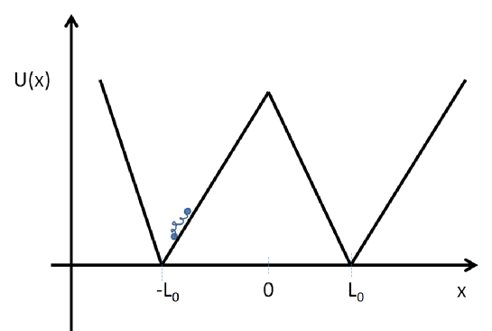
Figure 1: Schematic diagram for a dimer walking on a piecewise linear bistable potential. The potential wells and the barrier top are located at $x=\pm L_{0}$ and $x=0$, respectively. The dimer is initially situated at $x=-L_{0}$.

2 The model and effective potential

We consider a dimer of harmonic chain of two beads (monomers) which undergoes a Brownian motion along a ratchet potential where each bead has a friction coefficient $\gamma$ as shown in Fig. 1. The dynamics of the two beads is governed by the Langevin equation,

$$\gamma{dx_{1}\over dt}=-k(x_{1}-x_{2})-{\partial U(x_{1})\over\partial x_{1}}+\xi_{1}(t)$$ (1)

and

$$\gamma{dx_{2}\over dt}=-k(x_{2}-x_{1})-{\partial U(x_{2})\over\partial x_{2}}+\xi_{2}(t)$$ (2)

where the $k$ is the spring (elastic constant) of the dimer. The random force $\xi_{n}(t)$ is considered to be Gaussian and white noise satisfying

$$\left\langle\xi_{n}(t)\right\rangle=0,~{}~{}~{}\left\langle\xi_{n}(t)\xi_{n}(t+\tau)\right\rangle=2D\gamma\delta(\tau)$$ (3)

where $D=k_{B}T$ is the strength of the thermal noise. The rest length between the two monomer $l$ is assumed to be much less than the potential width, $l\ll 2L_{0}$ where $2L_{0}$ denotes the length of the ratchet potential. The piecewise linear bistable potential energy that the two bead experience is given by

$$U(x_{i})=U_{0}({{x_{i}\over L_{0}}}+1)-2U_{0}({x_{i}\over L_{0}})\Theta(x_{i})$$ (4)

where $i=1,2$ and $\Theta(x_{i})$ is the Heaviside function. The potential minima are located at $x=\pm L_{0}$ while the barrier of height $U_{0}$ is centered at $x=0$. For simplicity, we now introduce dimensionless rescaled barrier height ${\bar{U}_{0}}=U_{0}/D$ and rescaled length ${\bar{x}}=x/L_{0}$. We also introduced a dimensionless coupling strength ${\bar{k}}=kL_{0}^{2}/D$ and time ${\bar{t}}=t/\beta$ where $\beta=\gamma L_{0}^{2}/D$ denotes the relaxation time. In terms of the rescaled parameters Eq. (4) is rewritten as $U(x_{i})=U_{0}({x_{i}}+1)-2U_{0}(x_{i})\Theta(x_{i}).$

The corresponding Fokker Planck equation for Eqs. (1) and (2) is given by

$${\partial\over dt}P(x_{1},x_{2},t)={\partial\over\partial x_{1}}\chi_{1}P(x_{1},x_{2},t)+{\partial\over\partial x_{2}}\chi_{2}P(x_{1},x_{2},t)$$ (5)

where

$$\chi_{1}=k(x_{1}-x_{2})+{\partial U(x_{1})\over\partial x_{1}}+{\partial\over\partial x_{1}}$$ (6)

and

$$\chi_{2}=k(x_{2}-x_{1})+{\partial U(x_{2})\over\partial x_{2}}+{\partial\over\partial x_{2}}.$$ (7)

In large $k$ limit, the center mass motion (CM) $x_{cm}=(x_{1}+x_{2})/2$ of the dimer is significantly slow compared to the relative motion $y=(x_{2}-x_{1})/2$. Our aim is here is to get rid of the fast changing variable and to write an effective CM equation.

Before we do any analysis, next let us rewrite Eq. (5) in terms of the relative $y$ and the center of mass coordinate $x_{cm}$. Noting that for a rigid dimer $U(x_{2})-U(x_{1})\approx 0$, one gets

$${\partial P\over\partial t}={1\over 4}{\partial\over\partial x_{cm}}\left({\partial\over\partial x_{cm}}\left(U(x_{cm}-y)+U(x_{cm}+y)\right)P\right)+{1\over 2}{\partial^{2}P\over\partial x_{cm}^{2}}$$

$$+{1\over 4}{\partial\over\partial y}\left({\partial\over\partial y}\left(U(x_{cm}-y)+U(x_{cm}+y)\right)P\right)+{1\over 2}{\partial^{2}P\over\partial y^{2}}+$$ (8)

$${\partial\over\partial y}\left(kyP\right).$$

Once again ${\partial\over\partial y}\left(U(x_{cm}-y)+U(x_{cm}+y)\right)$ is negligible since for large $k$, $y=(x_{2}-x_{1})/2\approx 0$ and hence Eq. (8) is simplified to

$${\partial P\over\partial t}={1\over 4}{\partial\over\partial x_{cm}}\left({\partial\over\partial x_{cm}}\left(U(x_{cm}-y)+U(x_{cm}+y)\right)P\right)+{1\over 2}{\partial^{2}P\over\partial x_{cm}^{2}}$$

$$+{1\over 2}{\partial^{2}P\over\partial y^{2}}+{\partial\over\partial y}\left(kyP\right).$$ (9)

Introducing a rescaled relative term [5] ${\bar{y}}=y\sqrt{k}$ and ignoring the bar hereafter, the Fokker Planck equation (9) is rewritten as

$${\partial P\over\partial t}={\partial\over\partial x_{cm}}\left(A^{\prime}P\right)+{1\over 2}{\partial^{2}P\over\partial x_{cm}^{2}}+k{\partial\over\partial y}\left(yP+{1\over 2}{\partial P\over\partial y}\right)$$ (10)

where $A^{\prime}=(U^{\prime}(x_{cm}-{y\over\sqrt{k}})+U^{\prime}(x_{cm}+{y\over\sqrt{k}}))/4.$ By integrating out the $y$ degree of freedom, we project $P(x_{cm},y,t)$ into $P(x_{cm},t)$ as $P(x_{cm},t)=\int P(x_{cm},y,t)dy.$ Let us expand

$$P(x_{cm},y,t)=\sum_{n}P_{n}(x_{n},t)\psi_{n}(y,x_{cm})$$ (11)

where $\psi_{n}(y,x_{cm})$ is the Eigenfunction of

$${\partial\over\partial y}\left(y\psi_{n}(y,x_{cm})+{1\over 2}{\partial\over\partial y}\psi_{n}(y,x_{cm})\right)=-\lambda_{n}\psi_{n}(y,x_{cm}).$$ (12)

Here the eigenvalue $\lambda_{0}=0$ and $\lambda_{n}>0$ when $n\neq 0$. Thus

$${\partial\over\partial y}\left(y\psi_{0}(y,x_{cm})+{1\over 2}{\partial\over\partial y}\psi_{0}(y,x_{cm})\right)=0.$$ (13)

Solving for $\psi_{0}(y,x_{cm})$, we get

$$\psi_{0}(y,x_{cm})=\exp\left(-y^{2}\right)/\sqrt{\pi}.$$ (14)

Employing the adiabatic elimination method that explored in the work [5], one writes the effective Fokker Planck equation as

$${\partial P_{0}(x_{cm},t)\over\partial t} = {\partial\over\partial x_{cm}}\left\{\int A^{\prime}\psi_{0}dy\right\}P_{0}(x_{cm},t)+{D\over 2}{\partial^{2}\over\partial x_{cm}^{2}}\left\{\int\psi_{0}dy\right\}P_{0}(x_{cm},t)$$ (15)

$$= {\partial\over\partial x_{cm}}V^{\prime eff}(x_{cm})P_{0}(x_{cm},t)+{D\over 2}{\partial^{2}P_{0}(x_{cm},t)\over\partial x_{cm}^{2}}$$

where

$$V^{\prime eff}(x_{cm})=\int_{-\infty}^{\infty}\psi_{0}(y,x_{cm})A^{\prime}dy.$$ (16)

Here for the ratchet potential that we considered:

$$U\left(x_{cm}-{y\over\sqrt{k}}\right)=U_{0}\left(1+x_{cm}-{y\over\sqrt{k}}\right)-2U_{0}\left(x_{cm}-{y\over\sqrt{k}}\right)\Theta\left[x_{cm}-{y\over\sqrt{k}}\right],$$

$$U\left(x_{cm}+{y\over\sqrt{k}}\right)=U_{0}\left(1+x_{cm}+{y\over\sqrt{k}}\right)-2U_{0}\left(x_{cm}+{y\over\sqrt{k}}\right)\Theta\left[x_{cm}+{y\over\sqrt{k}}\right],$$

$$U^{\prime}\left(x_{cm}-{y\over\sqrt{k}}\right)=U_{0}-2U_{0}\left(x_{cm}-{y\over\sqrt{k}}\right)\delta\left[x_{cm}-{y\over\sqrt{k}}\right]-2U_{0}\Theta\left[x_{cm}-{y\over\sqrt{k}}\right],$$

and

$$U^{\prime}\left(x_{cm}+{y\over\sqrt{k}}\right)=U_{0}-2U_{0}\left(x_{cm}+{y\over\sqrt{k}}\right)\delta\left[x_{cm}+{y\over\sqrt{k}}\right]-2U_{0}\Theta\left[x_{cm}+{y\over\sqrt{k}}\right].$$ (17)

Substituting the above equations in Eq. (16) leads to

$$V^{\prime eff}(x_{cm})=-{U_{0}\over 4}Erf\left[x_{cm}/{\sqrt{k}}\right].$$ (18)

For any arbitrary small $x$, $Erf(x)\approx 2x/\sqrt{\pi}-2x^{3}/(3\sqrt{\pi})$. Hence $k$ is large, $V^{\prime eff}(x_{cm})$ is approximated as

$$V^{\prime eff}(x_{cm})=-{U_{0}\over 4}\left(\frac{2x_{cm}}{\sqrt{k\pi}}-\frac{2x_{cm}^{3}}{3\sqrt{\pi}k^{3/2}}\right).$$ (19)

The effective potential energy

$$V^{eff}(x_{cm}) = \int_{0}^{x_{cm}}V^{\prime eff}(x^{\prime}_{cm})dx^{\prime}_{cm}$$ (20)

$$= {U_{0}x_{cm}^{2}(-6k+x_{cm}^{2})\over 24k^{3/2}\sqrt{\pi}}$$

has potential minima at $x_{cm}=x^{\prime}_{m}=\pm\sqrt{3k}$ and maximum at $x_{cm}=0$. The shape of the effective potential strictly relies on the coupling strength and as well as on the barrier height of the ratchet potential as depicted in Figs. 2a and 2b.

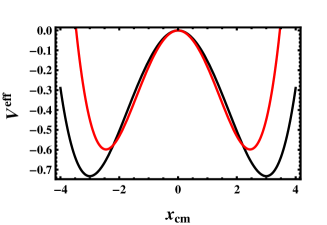
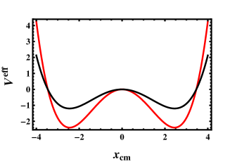
Figure 2: (color online) (a) The effective potential energy as a function of $x_{cm}$ for parameter choice $U_{0}=0.5$. The red and black lines stand for $k=1$ and $k=1.5$, respectively. (b) The effective potential energy as a function of $x_{cm}$ for parameter choice $k=1$ (red line stands for $U_{0}=2$ and black line for $U_{0}=1$)

.

3 The escape rate of the dimer in high barrier limit

Consider a dimeric molecule that initially situated at the potential minima of the bistable ratchet potential. At a frozen background temperature, the chain remains at its initial position and only when the temperature is above the frozen state that the dimer undergoes unbiased random walk along the reaction coordinate. In this case, unlike a point particle, its flexibility has nontrivial effects on its escaping rate. The shape of the potential profile and the strength of the thermal background kicks have also a pronounced effect on its barrier crossing rate.

In order to examine the various features of the rate in the regime of large $k$, we systematically trace out the fast changing relative term which leads to an effective Kramers type potential. For the chain that hops in the Kramers type of effective potential, the crossing rate in high barrier limit $\nabla V^{eff}\gg k_{B}T$ is approximated as [6] as

$$R={\sqrt{|\omega_{0}||\omega_{x_{m}^{{}^{\prime}}}|}\over 2\pi}e^{-2\nabla V^{eff}}.$$ (21)

where the effective barrier height $\nabla V^{eff}$ is the difference between the potential energy at the saddle point and the stable point $\nabla V^{eff}=V^{eff}(0)-V^{eff}(-x_{m})$. After some algebra we get $\nabla V^{eff}=\frac{3\sqrt{k}U_{0}}{8\sqrt{\pi}}$. The parameters $\omega_{0}$ and $\omega_{x_{m}}$ denote the curvature at the barrier top and the well minimum. We find $\omega_{0}=-U_{0}/(2\sqrt{k\pi})$ and $\omega_{x_{m}}=U_{0}/(\sqrt{k\pi})$. Note that limit $\nabla V^{eff}\gg k_{B}T$ for large $k$ and $U_{0}$.

To verify whether the results shown by the adiabatic elimination method holds true, we compute the rate as a function of coupling constant and barrier height via Brownian dynamic simulations. In the simulations, an initially coiled dimer is situated in one of the potential minima of a piecewise linear bistable potential. The trajectory for the center of mass and relative motion is simulated by considering different time steps $t$ and time lengths $t_{max}$. The numerical accuracy is taken care of by taking a large number of ensembles.

In Fig. 3a, we plot the rate as a function of $k$. The dotted line is evaluated via the numerical simulation while the solid line is from analytical prediction. In both cases, the rate monotonously decreases as $k$ steps up which agrees with the work [5]. In the high barrier limit (when $k$ is large), the simulation result approaches to the analytic one as expected. The dependence of the rate on the rescaled barrier height $U_{0}$ is depicted in Fig. 3b. The simulation (dotted line) as well as the approximation (solid line) results reveal that the rate has an optimal value at a certain $U_{0}$. For large $U_{0}$ (high barrier limit), both curves approach to each other.

Figure 3: (a) Dimer crossing rate $R$ as a function of coupling constant $k$ for fixed $U_{0}=6.0$. The dotted line depicts the rate evaluated via simulation while the solid line indicates the rate from analytical prediction. (b) The rate $R$ versus $U_{0}$ for parameter choice $k=3.0$. The dotted and solid lines depict the rate evaluated analytically and via numerical simulation, respectively. The rate attains an optimum value at a certain $U_{0}$.

Note that for sufficiently small $k$, the rate $R$ exhibits an optimal value. However, this regime cannot be conceived by our present approach as it is only valid in the firm $k$ regime. At this point we want also to stress that the flexibility of the dimer experimentally can be altered by various ways. It is known that the hydrogen bonds firmly join the chain of the dimer (kinesin) or polymers. Because the flexibility of the dimer is restricted by the bond forces, breaking the hydrogen bonds may increase the rotational degree of freedom for each atom and thereby increases the macroscopic flexibility of the dimer [25, 26]. Moreover, hydrogen bonds, being the weakest bonds in comparison to the covalent or ionic bonds, they can be easily broken by thermal and chemical denaturalization which dramatically increases the chains elasticity. The method of altering the protein flexibility via ligand binding is also discussed in the work [27]. In addition, the increased flexibility due to attenuated repulsions of some polymers such as DNA is reported in the work [28]. The repulsion between phosphates along the double helix contributes to the stiffness of the DNA. Introducing positively charged surfaces increases the flexibility of DNA as it renormalizes the repulsion between the two helixes. Since, the two lobes of the dimer are mediated by flexible protein, these all novel methods of manipulating the elasticity of the proteins is vital for fabrication of a dimer of a specific coupling strength that can be transported rapidly to a desired region

4 Signal to noise ratio

In the presence of time varying force, the system reaction to the external stimulation may depend on the flexibility of the dimer, shape of the potential profile and on the strength of the noise. Next we study the dependence of the SR on these model parameters employing two state approximation for large coupling constant $k$.

In the presence of periodic signal $A_{0}\cos{(\Omega t)}$, the dynamics of the system is governed by

$$\gamma{dx_{1}\over dt}=-k(x_{1}-x_{2})-{\partial U(x_{1})\over\partial x_{1}}+{\bar{A}}_{0}\cos(\Omega t)+\xi_{1}(t)$$ (22)

and

$$\gamma{dx_{2}\over dt}=-k(x_{2}-x_{1})-{\partial U(x_{2})\over\partial x_{2}}+{\bar{A}}_{0}\cos(\Omega t)+\xi_{2}(t)$$ (23)

where ${\bar{A}}_{0}$ and $\Omega$ denote the amplitude the angular frequency, respectively. Here ${\bar{A}}_{0}=A_{0}L_{0}/D$ and the bar will be dropped from now on.

Employing two state model approach [10, 24], the expression for signal to noise ratio for the chain has been derived in the work [10, 5]. Following the same approach, for sufficiently small amplitude, one finds the signal noise ratio

$$SNR=\pi R(2A_{0})^{2}$$ (24)

where the rate $R$ is evaluated via adiabatic elimination of fast variable.

In Figure 4, the plot of SNR as a function of $U_{0}$ is presented. Both the simulation (dotted line) and the analytic (solid line) findings show that the SNR steps up with $U_{0}$ and manifest a maximum value at a particular $U_{0}$. Further increasing in $U_{0}$ results in a smaller SNR. The same figure depicts that, for large $U_{0}$, both lines approach to each other.

Figure 4: The dependence of $SNR$ as a function of noise strength $U_{0}$ for a given amplitude $A_{0}=0.1$ and $k=3$ (dotted line from simulation while solid line from analytic prediction ). The figure exhibits that the $SNR$ increases as $U_{0}$ increases and then attains an optimal value at an optimal $U_{0}$.

5 Summary and conclusion

In summary, considering an initially coiled dimer which initially situated in the vicinity of the potential minima of a piecewise linear bistable potential, the thermally activated rate is explored as a function a rescaled barrier height $U_{0}$. It is shown that the rate monotonously increases with $U_{0}$ and attains a maximum value. Further increasing in $U_{0}$ leads to a smaller rate. The plot of $R$ as a function of $k$ also shows that when $k$ increases, the rate decreases. Furthermore, the response of the chain to time varying force is explored. In this case utilizing the two state approximation, the dependence of SNR as a function $U_{0}$ and $k$ is explored. In this case SNR exhibits an optimal value at optimal $U_{0}$.

This theoretical study is crucial since the complicated dynamics of most of biological systems can be effectively studied by mapping into two coupled bodies. The result obtained in this theoretical work can be also checked experimentally. One makes negatively charged dimer (coupled proteins), then put the dimer within positively and negatively charged fluidic channel where the fluidic channel is subjected to an external periodic force (AC field). At low temperature, the dimer prefers to stay at a positively charged part of the channel. However, due to thermal fluctuations as well as conformational change of the monomers, the dimer may presumably cross the high potential barrier.

In conclusion, since the dynamics of complicated system such as polymer and membranes not only relies on shape of the external potential but also on their system size, studying their dynamics is quiet complicated. However, one can simplify the problem by reducing the $N$ degree of freedoms into an effective two body problem such as dimer. This implies that the dimer serves as a basic model to understand the complicated dynamics of biological systems. Thus we believe that the present theoretical study is crucial for the fundamental understanding of polymer and membrane physics.

References

- [1] P.J. Park and W. Sung, J. Chem. Phys. 111, 5259 (1999).
- [2] S. Lee and W. Sung, Phys. Rev. E 63, 021115 (2001).
- [3] K.L. Sebastian and Alok K.R. Paul, Phys. Rev. E 62, 927 (2000).
- [4] M. Asfaw , Phys. Rev. E, 82, 021111 (2010).
- [5] M. Asfaw and Y. Shiferaw, JCP 136,025101(2012).
- [6] P. Hänggi, P. Talkner and M. Borkovec, Rev. Mod. Phys. 62, 251 (1990).
- [7] P. Hänggi, F. Marchesoni and P. Sodano, Phys. Rev. Lett. 60, 2563 (1988).
- [8] F. Marchesoni, C. Cattuto and G. Costantini, Phys. Rev. B, 57, 7930 (1998).
- [9] R. Benzi, G. Parisi, A. Sutera and A. Vulpiani, Tellus 34, 10 (1982).
- [10] L. Gammaitoni, P. Hänggi, P. Jung and F. Marchesoni, Rev. Mod. Phys. 70, 223 (1998).
- [11] J. F. Lindner, B. K. Meadows, W. L. Ditto, M. E. Inchiosa, and A. R. Bulsara, Phys. Rev. Lett. 75, 3 (1995); Phys. Rev. E 53, 2081 (1996).
- [12] F. Marchesoni, L. Gammaitoni, and A. R. Bulsara, Phys. Rev. Lett. 76, 2609 (1996).
- [13] Igor E. Dikshtein, Dmitri V. Kuznetsov and Lutz Schimansky-Geier, Phys. Rev. E. 65, 061101 (1996).
- [14] M. Asfaw and W. Sung, EPL, 90, 3008 (2010).
- [15] P. S. Burada, G. Schmid, D. Reguera, M. H. Vainstein, J. M. Rubi, and P. Hänggi, Phys. Rev. Lett. 101, 130602 (2008).
- [16] A. Pototsky, F. Marchesoni, and S. E. Savel ev1, Phys.Rev. E 81,031114 (2010).
- [17] A. Pototsky, N. B. Janson, F. Marchesoni, S.E. Savel eva, Chem. Phys. 375,458 (2010).
- [18] E. Heinsalu, M. Patriarca, and F. Marchesoni, Phys.Rev. E 77,021129 (2008).
- [19] O. M. Braun,R. Ferrando and G. E. Tommei,Phys.Rev. E 68, 051101 (2003).
- [20] C. Fusco, A. Fasolino and T. Janssen Eur. Phys. J. B 31, 95 (2003).
- [21] E. Heinsalu, M. Patriarca, F. Marchesoni, Chem. Phys. 375,410 (2010).
- [22] K. Kaneko, Progress of Theoretical Physics. 66, 129 (1981).
- [23] H. Risken, The Fokker-Planck equation: Methods of solution and applications, 2nd ed., Springer-Verlag, Berlin, Heidelberg, 1989.
- [24] B. McNamara, K. Wiesenfeld, Phy. Rev. A, 39, 4854 (1989).
- [25] B. Schulze, A. Sljoka and W. Whiteley, AIP Proceedings of AMMCS 2011.
- [26] B. M. Hespenheid, A. J. Rader, M. F. Thorpe, L. A. Kuhn, J. Molec. Graphics and Modelling, 21, 195 (2002)
- [27] R. l Najmanovich, J. Kuttner, V. Sobolev, and M. Edelman, PROTEINS: Structure, Function, and Genetics, 39, 261 (2000).
- [28] A. Podest , M. Indrieri , D. Brogioli, G. S. Manning, P. Milani, R. Guerra, L. Finzi, D. Dunlap, Biophysical Journal 89 2558, (2005).