Doorway States in the Random-Phase Approximation

Abstract

By coupling a doorway state to a sea of random background states, we develop the theory of doorway states in the framework of the random-phase approximation (RPA). Because of the symmetry of the RPA equations, that theory is radically different from the standard description of doorway states in the shell model. We derive the Pastur equation in the limit of large matrix dimension and show that the results agree with those of matrix diagonalization in large spaces. The complexity of the Pastur equation does not allow for an analytical approach that would approximately describe the doorway state. Our numerical results display unexpected features: The coupling of the doorway state with states of opposite energy leads to strong mutual attraction.

1 Introduction

In the description of nuclear-structure phenomena, doorway states play an important role. Standard examples are the giant-dipole resonance [1] and, in medium-weight nuclei, low-lying isobaric analogue states [2]. A doorway state occurs when a distinct mode of nuclear excitation of given spin and parity, coupled strongly to the nuclear ground state or to some distinct scattering channel, is mixed with a background of states with the same quantum numbers. The strength of the mixing determines the spreading width of the ensuing resonance. For the giant-dipole resonance in even-even nuclei, the mode has spin/parity $1^{-}$ and is strongly coupled through the dipole operator to the nuclear ground state. The background states also have spin/parity $1^{-}$. The resonance shows up in the cross section for photon absorption. The isobaric analogue state has isospin $T_{0}+1$ and is strongly coupled to the channel for scattering of protons on a target nucleus with one less proton. The background states have isospin $T_{0}$. The isobaric analogue resonance shows up in elastic proton scattering. Doorway states play an important role also in other areas of physics. By way of example we mention quantum information theory, mesoscopic physics, quantum chaos, and molecular physics. Without aiming at completeness, we refer to Refs. [3, 4, 5, 6, 7, 8, 9, 10] and references therein.

In the standard theoretical description (see Ref. [11] and references therein), the doorway mode has energy $E_{0}$ and is coupled through real matrix elements $V_{\mu}$, $\mu=1,\ldots,N$ to $N$ background states. These are governed by a real and symmetric Hamiltonian matrix $h_{\mu\nu}$ with $\mu,\nu=1,\ldots,N$. In matrix form the total Hamiltonian $H$ is given by

$$H=\left(\matrix{E_{0}&V_{\nu}\cr V_{\mu}&h_{\mu\nu}\cr}\right)\ .$$ (1)

(For isobaric analogue resonances, Eq. (1) must be generalized to include the coupling of the analogue state with the background states via the proton channel, see Ref. [11].) Eq. (1) is patterned after the nuclear shell model. There, the dipole mode would be a linear superposition of one-particle one-hole states, the background states would be two-particle two-hole states, and $E_{0}$, the $V_{\mu}$ and the elements $h_{\mu\nu}$ would be determined by the single-particle energies and the residual interaction. For $N\gg 1$ a dynamical theory of the background states is not available in most cases, however, and the Hamiltonian matrix $h$ is replaced by a matrix drawn at random from the Gaussian Orthogonal Ensemble of real symmetric matrices (the GOE). We have addressed the resulting problems in the theory of doorway states in two recent papers. In Ref. [12], we have worked out in a very general framework properties of doorway states as averages over the GOE in the limit $N\to\infty$. Properties of the spreading width that emerge beyond the standard approximation were investigated in Ref. [13]. An essential and generic feature of the doorway state model is that the value of the spreading width is adjustable. Moreover, this value is of order $1/N$ in relation to the overall width of the spectrum of the background states. This last property guarantees that the doorway state is a local spectral phenomenon.

In the present paper we extend the concept and the description of doorway states to the random-phase approximation (RPA). Our extension is motivated by the fact that in nuclear-structure theory, it is often mandatory to replace the shell-model approach embodied in Eq. (1) by the RPA [14]. That is true especially for the treatment of collective motion. The RPA is characterized by symmetries that are radically different from those of the Hamiltonian approach in Eq. (1). Our extension takes account of these symmetries. Specifically, it involves four elements. (i) We need an RPA model for the doorway state as a collective state. (ii) Similar to the replacement of $h_{\mu\nu}$ by the GOE, our RPA model must involve a random-matrix model with RPA symmetries for the background states. (iii) The coupling of the doorway state to the background states (the analogue of the matrix elements $V_{\mu}$) must also possess RPA symmetries. (iv) The value of the spreading width due to that coupling must be an adjustable parameter, and it must be of order $1/N$ in relation to the overall width of the spectrum of the background states. The resulting theory of the doorway phenomenon in RPA turns out to be radically different from the standard approach.

The random-matrix approach to RPA equations has been formulated and investigated in some detail in Ref. [15]. In that paper a follow-up paper was announced that would combine the purely statistical (or “democratic”) description of the background states in terms of a random-matrix model with the highly special dynamical RPA description of a select state, the doorway state. Aside from being an extension of our investigation of the doorway state phenomenon in Refs. [12, 13], the present paper may also be viewed as that follow-up paper. It might, therefore, also carry the title “Random-Matrix Approach to RPA Equations II”. In the paper we are mainly interested in the consequences the RPA symmetry has for the doorway state picture. We do not discuss any applications.

2 RPA

For a set of $N$ degenerate shell-model states with energy $r$, the RPA equations have the form [14]

$${\cal H}^{(0)}X^{\nu}=(E_{\nu}-E_{0})X^{\nu}$$ (2)

where

$${\cal H}^{(0)}=\left(\matrix{r{\bf 1}_{N}+A&C\cr-C^{*}&-r{\bf 1}_{N}-A^{*}\cr}\right)\ .$$ (3)

In Eq. (2) $E_{0}$ ($E_{\nu}$) is the energy of the ground state (one of the excited states, respectively). The eigenvectors $X^{\nu}$ have dimension $2N$. In Eq. (3) ${\bf 1}_{N}$ is the unit matrix in $N$ dimensions. The matrices $A$ and $C$ represent the residual interaction and have dimension $N$ each. For time-reversal invariant systems (orthogonal case), both $A$ and $C$ are real symmetric matrices. If time reversal invariance is violated (unitary case), the matrix $A$ is Hermitean and the matrix $C$ is complex symmetric. The symmetries of the matrices $A$ and $C$ imply that if ${\cal E}_{\nu}=E_{\nu}-E_{0}$ is an eigenvalue of the RPA equations (2), then ${\cal E}^{*}_{\nu}$, $-{\cal E}_{\nu}$, and $-{\cal E}^{*}_{\nu}$ are also eigenvalues. These symmetries of ${\cal H}^{(0)}$ are caused by the RPA approximation. As a consequence, the RPA matrix in Eq. (3) is not Hermitean and, therefore, does not correspond to any Hamiltonian. That is why the random-matrix approach developed in Ref. [15] does not correspond to any of the generalized random-matrix ensembles introduced by Altland and Zirnbauer [16].

We now address point (i) of Section 1 and recall the construction of a collective RPA state. That state will serve as the doorway state. In the schematic model, such a collective state emerges from the set of $N$ degenerate shell-model states if the interaction is separable, i.e., if the RPA matrix in Eq. (3) is of the form

$$\left(\matrix{r\delta_{\mu\nu}+a_{\mu}a^{*}_{\nu}&a_{\mu}a_{\rho}\cr-a^{*}_{\sigma}a^{*}_{\nu}&-r\delta_{\sigma\rho}-a^{*}_{\sigma}a_{\rho}\cr}\right)\ .$$ (4)

The indices $\mu$ and $\nu$ ($\rho$ and $\sigma$) run from $1$ to $N$ (from $N+1$ to $2N$, respectively). The symmetry of the RPA equations implies $a_{\mu}=a_{N+\mu}$ for all $\mu=1,\ldots,N$. The quantities $a_{\mu}$ with $\mu=1,\ldots,N$ are complex in the unitary case and real in the orthogonal case. In the schematic model one often uses a common factor multiplying each of the four separable matrices. The sign of that factor determines whether the energy of the collective state is raised or lowered. We omit that factor in order not to introduce too much complexity. The relative strengths of the four separable matrices are fixed. This is neccessary for the schematic model to yield a truly collective state. It is straightforward to solve the RPA equations for the schematic model (4). The collective state is located at energies $\pm[r^{2}+2r\sum_{\mu=1}^{N}|a_{\mu}|^{2}]^{1/2}$ while the remaining $2(N-1)$ states retain their unperturbed energies $\pm r$.

We turn to point (ii) of Section 1 and recall the random-matrix approach to the RPA of Ref. [15]. There it was assumed that both $A$ and $C$ are random matrices. With the same notation as used for the RPA matrix (4) we write the RPA matrix (3) as

$$\left(\matrix{r\delta_{\mu\nu}+A_{\mu\nu}&C_{\mu\rho}\cr-C^{*}_{\sigma\nu}&-r\delta_{\sigma\rho}-A^{*}_{\sigma\rho}\cr}\right)\ .$$ (5)

The indices $\mu,\nu$ ($\rho,\sigma$) run from $1$ to $N$ (from $N+1$ to $2N$, respectively). Moreover we have $A_{(\mu+N)(\nu+N)}=A_{\mu\nu}$ and $C_{\mu(\nu+N)}=C_{\mu\nu}$. The independent elements of the matrices $A$ and $C$ are assumed to be uncorrelated Gaussian–distributed random variables with zero mean values and second moments given by

$$\langle A_{\mu\nu}A_{\mu^{\prime}\nu^{\prime}}\rangle = \frac{\lambda^{2}}{N}\delta_{\mu\mu^{\prime}}\delta_{\nu\nu^{\prime}}\ {\rm(unitary\ case),\ or}$$

$$\langle A_{\mu\nu}A_{\mu^{\prime}\nu^{\prime}}\rangle = \frac{\lambda^{2}}{N}(\delta_{\mu\mu^{\prime}}\delta_{\nu\nu^{\prime}}+\delta_{\mu\nu^{\prime}}\delta_{\nu\mu^{\prime}})\ {\rm(orthogonal\ case),\ and}$$

$$\langle C_{\mu\nu}C^{*}_{\mu^{\prime}\nu^{\prime}}\rangle = \frac{\gamma^{2}}{N}(\delta_{\mu\mu^{\prime}}\delta_{\nu\nu^{\prime}}+\delta_{\mu\nu^{\prime}}\delta_{\mu^{\prime}\nu})\ ;\ \langle C_{\mu\nu}C_{\mu^{\prime}\nu^{\prime}}\rangle=0\ {\rm(unitary\ case),\ or}$$

$$\langle C_{\mu\nu}C_{\mu^{\prime}\nu^{\prime}}\rangle = \frac{\gamma^{2}}{N}(\delta_{\mu\mu^{\prime}}\delta_{\nu\nu^{\prime}}+\delta_{\mu\nu^{\prime}}\delta_{\nu\mu^{\prime}})\ {\rm(orthogonal\ case)}\ .$$ (6)

In Eqs. (6) all indices run from $1$ to $N$. For $\gamma=0$ and $r>2\lambda$ the average RPA spectrum consists of two semicircles with equal radii $2\lambda$ centered at $\pm r$. Non-zero values of the parameter $\gamma$ cause attraction between states with positive and negative energy and, with increasing $\gamma$, eventually lead to coalescence of a first pair of levels with opposite signs at energy $E=0$. That is the point of instability of the RPA equations. A further increase of $\gamma$ leads to complex eigenvalues. In Ref. [15] values of $\gamma$ at the instability point are given as functions of the parameters $r$ and $\lambda$.

Concerning point (iii) of Section 1 there are two alternative ways of coupling the doorway state emerging from Eqs. (2), (3) and (4) to the background states described by Eqs. (2), (3), (5), and (6).

2.1 Strong-Coupling Model

We combine the schematic model (4) for the doorway state with the random RPA model of Eqs. (5) and (6) and write the $2N$–dimensional RPA matrix ${\cal H}$ as

$${\cal H}=\left(\matrix{r\delta_{\mu\nu}+a_{\mu}a^{*}_{\nu}+A_{\mu\nu}&a_{\mu}a_{\rho}+C_{\mu\rho}\cr-a^{*}_{\sigma}a^{*}_{\nu}-C^{*}_{\sigma\nu}&-r\delta_{\rho\sigma}-a^{*}_{\sigma}a_{\rho}-A^{*}_{\sigma\rho}\cr}\right)\ .$$ (7)

The matrices $A$ and $C$ are taken to be members of the random-matrix ensembles defined in and below Eqs. (6). Eq. (7) can be interpreted by saying that the matrix elements of the two–body interaction in the RPA approach partly factorize, giving rise to the separable matrices $a_{\mu}a^{*}_{\nu}$ etc., while the remaining parts of these matrix elements are replaced by random variables. That seems a very natural choice of introducing both, a distinct doorway state and a random-matrix description of the remaining background states. Moreover, the strong-coupling model of Eq. (7) has the advantage of carrying a small number of parameters. Unfortunately these advantages are overcompensated by the fact that in the strong-coupling model, the spreading width of the doorway state is fixed and given by the radius $2\lambda$ of the semicircle, i.e., of the average spectrum of background states. We demonstrate that fact in the appendix. Because of this shortcoming of the strong-coupling model we devote the remainder of the paper entirely to the variable-coupling model.

2.2 Variable-Coupling Model

In order to accommodate both, a set of $N$ random background states and a collective state with variable coupling to these states, we choose the RPA matrix ${\cal H}$ to have dimension $2N+2$. We label the first row and column with the letter $\alpha$, the following $N$ rows and columns with the indices $\mu,\nu=1,\ldots,N$, the next row and column with the letter $\beta$, and the remaining rows and columns with the indices $\rho,\sigma=N+1,\ldots,2N$. We write

$${\cal H}=\left(\matrix{r+|a|^{2}&v\delta_{\nu 1}&a^{2}&w\delta_{\rho(N+1)}\cr v^{*}\delta_{\mu 1}&r\delta_{\mu\nu}+A_{\mu\nu}&w\delta_{\mu 1}&C_{\mu\rho}\cr-(a^{*})^{2}&-w^{*}\delta_{\nu 1}&-r-|a|^{2}&-v^{*}\delta_{\rho(N+1)}\cr-w^{*}\delta_{\sigma(N+1)}&-C^{*}_{\sigma\nu}&-v\delta_{\sigma(N+1)}&-r\delta_{\sigma\rho}-A^{*}_{\sigma\rho}\cr}\right)\ .$$ (8)

The matrices $A$ and $C$ are random, with the same properties as described above. Comparison with expression (4) shows that the collective state is already in (almost) diagonal form. In the RPA matrix (8) the coupling to the background states is described by the two parameters $v$ and $w$ that occur in the rows and columns labelled $1$ and $N+1$. All other coupling matrix elements vanish. This simplified form of the RPA matrix (8) holds without loss of generality. It follows from the generalized orthogonal (unitary) invariance of the matrices $A$ and $C$. The parameters $v$ and $w$ are real (complex) in the orthogonal (unitary) case. The form of the RPA matrix (8) bears a direct analogy to the matrix on the right-hand side of Eq. (1). There is some similarity between the variable-coupling model of Eq. (8) and the strong-coupling model of Eq. (7) except that in the latter the doorway state is not afforded an extra dimension.

From the results of Ref. [15] we expect that for $C=0$, coalescence of eigenvalues of the variable-coupling model occurs only at $E=0$ and only as a consequence of level repulsion caused by $v$. To check this we put $C=0$. Since $A$ causes level repulsion, we also put $A=0$. In the resulting eigenvalue equation, $N-1$ of the degenerate positive eigenvalues remain located at $r$ while one is changed because of its interaction with the collective state. The same is true of the negative eigenvalues. The relevant part of the secular equation is

$$\det\left(\matrix{r+|a|^{2}-E&v&a^{2}&w\cr v^{*}&r-E&w&0\cr-(a^{*})^{2}&-w^{*}&-r-|a|^{2}-E&-v^{*}\cr-w^{*}&0&-v&-r-E\cr}\right)=0\ .$$ (9)

The solution of this quadratic equation in $E^{2}$ is

$$E^{2}=r^{2}+r|a|^{2}+|v|^{2}-|w|^{2}\pm\sqrt{D}\ .$$ (10)

The discriminant $D$ has the value

$$D=|a|^{4}r^{2}+4|v|^{2}r^{2}+4|v|^{2}|a|^{2}r-2r(a^{2}v^{*}w^{*}+{\rm c.c.})\ .$$ (11)

Two eigenvalues coalesce when $D=0$. For that to happen, the term $(a^{2}v^{*}w^{*}+{\rm c.c.})$ must be positive. With $\phi$ the phase angle between $a^{2}v^{*}$ and $w^{*}$ a zero of $D$ occurs if

$$|w|\cos\phi=\frac{(1/4)r|a|^{4}+|a|^{2}|v|^{2}+r|v|^{2}}{|a|^{2}|v|}\ .$$ (12)

Coalescence of two eigenvalues is physically relevant only if the coalescing eigenvalues are real. That is the case if

$$r^{2}+r|a|^{2}+|v|^{2}-|w|^{2}\geq 0\ .$$ (13)

We use in Eq. (13) the equality sign, take $w,a,v$ to be positive, and solve Eqs. (12) and (13) for $v^{2}$. That yields the two solutions $v^{2}_{1}=(a^{4}/4)(r/(r+2a^{2}))$ and $v^{2}_{2}=a^{4}/4$. Insertion shows that for both $v^{2}_{1}$ and $v^{2}_{2}$, the coinciding energy eigenvalues vanish. But for $v^{2}$ in the interval $v^{2}_{1}<v^{2}<v^{2}_{2}$, the coinciding eigenvalues are real and generically differ from zero. Choosing, for instance, $r=2$ and $a=0.5$, one finds $v_{1}=0.111803$ and $v_{2}=0.125$ so that for $v_{1}<v<v_{2}$ the coinciding eigenvalues differ from zero. For example, for $v=0.12$ one gets $E=0.113713$. The result is somewhat surprising: In the variable-coupling model, coincidence of two non-zero real eigenvalues is possible. This is in contrast to the random RPA model in Eq. (2) where coincidence of two real eigenvalues is possible only at $E=0$. The appearance of coinciding nonzero eigenvalues probably signals another breakdown point of the RPA. Indeed, the values of $w$ corresponding to $v_{1}$ and $v_{2}$ are $w_{1}=2.12426$ and $w_{2}=2.125$, respectively, much larger than $v_{1}$ or $v_{2}$ and, thus, perhaps unphysical.

3 Pastur Equation

We establish properties of the average spectrum of the variable-coupling model with the help of the Pastur equation. We follow Refs. [12, 15, 13] and for simplicity consider the unitary case only.

The Pastur equation is an equation for the average Green function, a matrix of dimension $2N+2$ given by

$$\langle G(E)\rangle=\bigg{\langle}\bigg{(}E^{+}{\bf 1}_{2N+2}-{\cal H}\bigg{)}^{-1}\bigg{\rangle}\ ,$$ (14)

with ${\cal H}$ defined in Eq. (8). The energy $E$ carries a positive imaginary increment. The angular brackets denote the ensemble average. To obtain an equation for $\langle G(E)\rangle$, we define the “unperturbed” Green function $G_{0}(E)$ by omitting from ${\cal H}$ the random matrices $A$ and $C$, and we expand $\langle G(E)\rangle$ around $G_{0}(E)$ in powers of $A$ and $C$. We take a term–by–term ensemble average of the resulting series, omitting terms that are small of order $1/N$, and we resum the result.

The non-statistical part of ${\cal H}$ is given by

$${\cal H}_{0}=\left(\matrix{r+|a|^{2}&v\delta_{\nu 1}&a^{2}&w\delta_{\rho(N+1)}\cr v^{*}\delta_{\mu 1}&r\delta_{\mu\nu}&w\delta_{\mu 1}&0\cr-(a^{*})^{2}&-w^{*}\delta_{\nu 1}&-r-|a|^{2}&-v^{*}\delta_{\rho(N+1)}\cr-w^{*}\delta_{\sigma(N+1)}&0&-v\delta_{\sigma(N+1)}&-r\delta_{\sigma\rho}\cr}\right)\ .$$ (15)

The random part ${\cal H}_{\rm r}$ is correspondingly given by

$${\cal H}_{\rm r}=\left(\matrix{0&0&0&0\cr 0&A_{\mu\nu}&0&C_{\mu\rho}\cr 0&0&0&0\cr 0&-C^{*}_{\sigma\nu}&0&-A^{*}_{\sigma\rho}\cr}\right)\ .$$ (16)

The unperturbed Green function is

$$G_{0}(E)=(E^{+}{\bf 1}_{2N+2}-{\cal H}_{0})^{-1}\ ,$$ (17)

and the Pastur equation reads

$$\langle G(E)\rangle=G_{0}(E)+G_{0}(E)\langle{\cal H}_{r}\langle G(E)\rangle{\cal H}_{r}\rangle\langle G(E)\rangle\ .$$ (18)

We define four projection operators, $Q_{1}$ and $Q_{2}$ as the projectors onto the subspaces spanned by the states labelled $1,2,\ldots,N$ and $N+1,N+2,\ldots,2N$, respectively, and $P_{\alpha}$ and $P_{\beta}$ as the projectors onto the states $\alpha$ and $\beta$, respectively. For $i=1,2$ we define

$$\sigma_{i}(E) = \frac{\lambda}{N}{\rm Trace}\ Q_{i}\langle G(E)\rangle Q_{i}\ ,$$

$$\delta = \frac{\gamma}{\lambda}\ ,$$

$$\Sigma_{i}(E) = \sigma_{i}-\delta^{2}\sigma_{i+1}\ ,$$

$$\sigma_{3} = \sigma_{1}\ .$$ (19)

Moreover we introduce

$$G^{(1)}_{0}(E) = Q_{1}G_{0}(E)+Q_{1}G_{0}(E)Q_{2}\frac{\lambda\Sigma_{2}}{1-\lambda\Sigma_{2}Q_{2}G_{0}(E)Q_{2}}Q_{2}G_{0}(E)\ ,$$

$$G^{(2)}_{0}(E) = Q_{2}G_{0}(E)+Q_{2}G_{0}(E)Q_{1}\frac{\lambda\Sigma_{1}}{1-\lambda\Sigma_{1}Q_{1}G_{0}(E)Q_{1}}Q_{1}G_{0}(E)\ .$$ (20)

Upon projection, the Pastur equation (18) yields the following four equations.

$$P_{\alpha}\langle G(E)\rangle P_{\alpha} = P_{\alpha}G_{0}(E)P_{\alpha}$$

$$\qquad+\lambda\Sigma_{1}P_{\alpha}G_{0}(E)Q_{1}\bigg{(}1-\lambda\Sigma_{1}G^{(1)}_{0}(E)Q_{1}\bigg{)}^{-1}G^{(1)}_{0}(E)P_{\alpha}$$

$$\qquad+\lambda\Sigma_{2}P_{\alpha}G_{0}(E)Q_{2}\bigg{(}1-\lambda\Sigma_{2}G^{(2)}_{0}(E)Q_{2}\bigg{)}^{-1}G^{(2)}_{0}(E)P_{\alpha}\ ,$$

$$P_{\beta}\langle G(E)\rangle P_{\beta} = P_{\beta}G_{0}(E)P_{\beta}$$

$$\qquad+\lambda\Sigma_{1}P_{\beta}G_{0}(E)Q_{1}\bigg{(}1-\lambda\Sigma_{1}G^{(1)}_{0}(E)Q_{1}\bigg{)}^{-1}G^{(1)}_{0}(E)P_{\beta}$$

$$\qquad+\lambda\Sigma_{2}P_{\beta}G_{0}(E)Q_{2}\bigg{(}1-\lambda\Sigma_{2}G^{(2)}_{0}(E)Q_{2}\bigg{)}^{-1}G^{(2)}_{0}(E)P_{\beta}\ ,$$

$$Q_{1}\langle G(E)\rangle Q_{1} = \bigg{(}1-\lambda\Sigma_{1}G^{(1)}_{0}(E)Q_{1}\bigg{)}^{-1}G^{(1)}_{0}(E)Q_{1}\ ,$$

$$Q_{2}\langle G(E)\rangle Q_{2} = \bigg{(}1-\lambda\Sigma_{2}G^{(2)}_{0}(E)Q_{2}\bigg{)}^{-1}G^{(2)}_{0}(E)Q_{2}\ .$$ (21)

Explicit calculation yields

$$(Q_{1}G_{0}(E)Q_{1})_{\mu\nu} = \delta_{\mu\nu}(G_{0}(E))_{\mu\mu}\ ,$$

$$(Q_{2}G_{0}(E)Q_{2})_{\rho\sigma} = \delta_{\rho\sigma}(G_{0}(E))_{\rho\rho}\ ,$$

$$(Q_{1}G_{0}(E)Q_{2})_{\mu\rho} = \delta_{\mu 1}\delta_{\rho(N+1)}(G_{0}(E))_{1(N+1)}\ ,$$

$$(Q_{2}G_{0}(E)Q_{1})_{\rho\mu} = \delta_{\mu 1}\delta_{\rho(N+1)}(G_{0}(E))_{(N+1)1}\ ,$$

$$(P_{\alpha}G_{0}(E)Q_{1})_{\alpha\mu} = \delta_{\mu 1}(G_{0}(E))_{\alpha 1}\ ,$$

$$(P_{\alpha}G_{0}(E)Q_{2})_{\alpha\rho} = \delta_{\rho(N+1)}(G_{0}(E))_{\alpha(N+1)}\ ,$$

$$(P_{\beta}G_{0}(E)Q_{1})_{\beta\mu} = \delta_{\mu 1}(G_{0}(E))_{\beta 1}\ ,$$

$$(P_{\beta}G_{0}(E)Q_{2})_{\beta\rho} = \delta_{\rho(N+1)}(G_{0}(E))_{\beta(N+1)}\ ,$$

$$(Q_{1}G_{0}(E)P_{\alpha})_{\mu\alpha} = \delta_{\mu 1}(G_{0}(E))_{1\alpha}\ ,$$

$$(Q_{2}G_{0}(E)P_{\alpha})_{\rho\alpha} = \delta_{\rho(N+1)}(G_{0}(E))_{(N+1)\alpha}\ ,$$

$$(Q_{1}G_{0}(E)P_{\beta})_{\mu\beta} = \delta_{\mu 1}(G_{0}(E))_{1\beta}\ ,$$

$$(Q_{2}G_{0}(E)P_{\beta})_{\rho\beta} = \delta_{\rho(N+1)}(G_{0}(E))_{(N+1)\beta}\ .$$ (22)

We use Eqs. (22) in Eqs. (20) and (21), define

$$(g_{1})^{-1} = 1-\lambda\Sigma_{1}(G_{0}(E))_{11}$$

$$-\lambda\Sigma_{1}(G_{0}(E))_{1(N+1)}\frac{\lambda\Sigma_{2}}{1-\lambda\Sigma_{2}(G_{0}(E)_{(N+1)(N+1)}}(G_{0}(E))_{(N+1)1}\ ,$$

$$(g_{2})^{-1} = 1-\lambda\Sigma_{2}(G_{0}(E))_{(N+1)(N+1)}$$ (23)

$$-\lambda\Sigma_{2}(G_{0}(E))_{(N+1)1}\frac{\lambda\Sigma_{1}}{1-\lambda\Sigma_{1}(G_{0}(E)_{11}}(G_{0}(E))_{1(N+1)}\ ,$$

and obtain

$$(Q_{1}\langle G(E)\rangle Q_{1})_{\mu\nu}=\delta_{\mu\nu}(1-\delta_{\mu 1})\frac{(G_{0}(E))_{\mu\mu}}{1-\lambda\Sigma_{1}(G_{0}(E))_{\mu\mu}}$$

$$\qquad+\delta_{\mu\nu}\delta_{\mu 1}g_{1}\bigg{(}(G_{0}(E))_{11}$$

$$\qquad+(G_{0}(E))_{1(N+1)}\frac{\lambda\Sigma_{2}}{1-\lambda\Sigma_{2}(G_{0}(E))_{(N+1)(N+1)}}(G_{0}(E))_{(N+1)1}\bigg{)}\ ,$$

$$(Q_{2}\langle G(E)\rangle Q_{2})_{\rho\sigma}=\delta_{\rho\sigma}(1-\delta_{\rho(N+1)})\frac{(G_{0}(E))_{\rho\rho}}{1-\lambda\Sigma_{2}(G_{0}(E))_{\rho\rho}}$$

$$\qquad+\delta_{\rho\sigma}\delta_{\rho(N+1)}g_{2}\bigg{(}(G_{0}(E))_{(N+1)(N+1)}$$

$$\qquad+(G_{0}(E))_{(N+1)1}\frac{\lambda\Sigma_{1}}{1-\lambda\Sigma_{1}(G_{0}(E))_{11}}(G_{0}(E))_{1(N+1)}\bigg{)}\ ,$$

$$\langle G(E)\rangle_{\alpha\alpha}=(G_{0}(E))_{\alpha\alpha}+\lambda\Sigma_{1}(G_{0}(E))_{\alpha 1}g_{1}\bigg{(}(G_{0}(E))_{1\alpha}$$

$$\qquad+(G_{0}(E))_{1(N+1)}\frac{\lambda\Sigma_{2}}{1-\lambda\Sigma_{2}(G_{0}(E))_{(N+1)(N+1)}}(G_{0}(E))_{(N+1)\alpha}\bigg{)}$$

$$\qquad+\lambda\Sigma_{2}(G_{0}(E))_{\alpha(N+1)}g_{2}\bigg{(}(G_{0}(E))_{(N+1)\alpha}$$

$$\qquad+(G_{0}(E))_{(N+1)1}\frac{\lambda\Sigma_{1}}{1-\lambda\Sigma_{1}(G_{0}(E))_{11}}(G_{0}(E))_{1\alpha}\bigg{)}\ ,$$

$$\langle G(E)\rangle_{\beta\beta}=(G_{0}(E))_{\beta\beta}+\lambda\Sigma_{1}(G_{0}(E))_{\beta 1}g_{1}\bigg{(}(G_{0}(E))_{1\beta}$$

$$\qquad+(G_{0}(E))_{1(N+1)}\frac{\lambda\Sigma_{2}}{1-\lambda\Sigma_{2}(G_{0}(E))_{(N+1)(N+1)}}(G_{0}(E))_{(N+1)\beta}\bigg{)}$$

$$\qquad+\lambda\Sigma_{2}(G_{0}(E))_{\beta(N+1)}g_{2}\bigg{(}(G_{0}(E))_{(N+1)\beta}$$

$$\qquad+(G_{0}(E))_{(N+1)1}\frac{\lambda\Sigma_{1}}{1-\lambda\Sigma_{1}(G_{0}(E))_{11}}(G_{0}(E))_{1\beta}\bigg{)}\ .$$ (24)

We take the trace of the first and the second of these equations and use the definitions (19). That yields

$$\sigma_{1}(E) = \frac{N-1}{N}\frac{\lambda}{E-r-\lambda\Sigma_{1}}+\frac{1}{N}\lambda g_{1}\bigg{(}(G_{0}(E))_{11}$$

$$\qquad+(G_{0}(E))_{1(N+1)}\frac{\lambda\Sigma_{2}}{1-\lambda\Sigma_{2}(G_{0}(E))_{(N+1)(N+1)}}(G_{0}(E))_{(N+1)1}\bigg{)}\ ,$$

$$\sigma_{2}(E) = \frac{N-1}{N}\frac{\lambda}{E+r-\lambda\Sigma_{2}}+\frac{1}{N}\lambda g_{2}\bigg{(}(G_{0}(E))_{(N+1)(N+1)}$$ (25)

$$\qquad+(G_{0}(E))_{(N+1)1}\frac{\lambda\Sigma_{1}}{1-\lambda\Sigma_{1}(G_{0}(E))_{11}}(G_{0}(E))_{1(N+1)}\bigg{)}\ .$$

Given the parameters $r,a,v,w$ we can calculate the matrix elements $(G_{0}(E))_{ij}$ with $i,j=\alpha,1,\beta,(N+1)$. Then Eqs. (25) together with the defining Eqs. (23) constitute a pair of non-linear coupled equations for the unknown functions $\sigma_{1}(E)$ and $\sigma_{2}(E)$. Once these are known, $\langle G(E)\rangle_{\alpha\alpha}$ and $\langle G(E)\rangle_{\beta\beta}$ are given by the last two Eqs. (24). The symmetry properties of the solutions of Eqs. (25) are the same as discussed in Section 6 of Ref. [15].

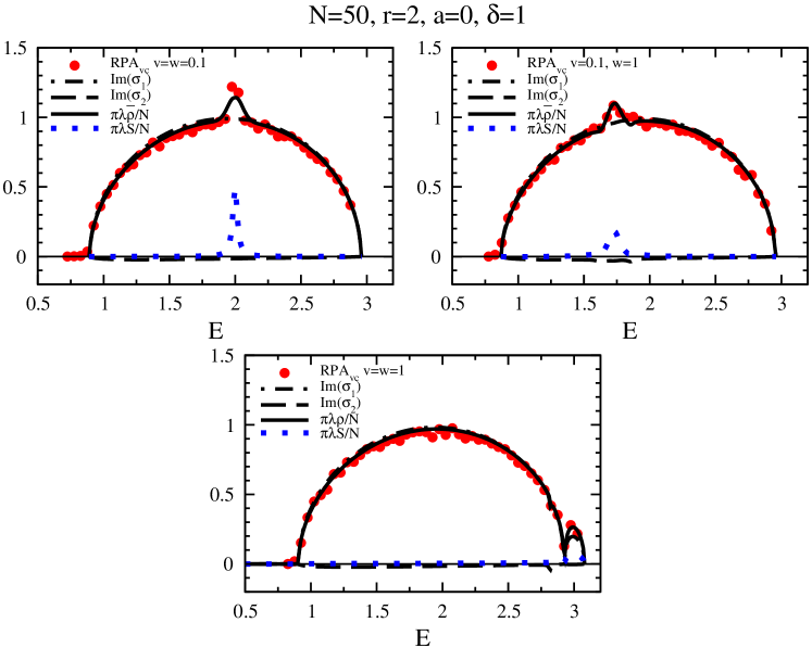
Figure 1: The dimensionless total level density as obtained from the Pastur equation (black line) and from matrix diagonalization (red dots) plus various contributions to the density (see text) for three values of $(v,w)$ as indicated in the figure.

To determine the average level density $\rho(E)=\rho(-E)$, we focus attention on the positive part of the spectrum. We expect that part to consist of up to three pieces, one due to the random part of ${\cal H}$, one due to the level with index $\alpha$, and one due to the level with index $1$. (That last level interacts strongly with level $\alpha$ and may be pushed outside the random part of the spectrum). The average Green function has up to three branch cuts along the positive real $E$ axis, each corresponding to one of these parts. We look for the solutions with negative imaginary parts on each of the cuts. For the solutions with $E<0$ we refer to the discussion in Section 6 of Ref. [15]. For $E>0$ the level density is given by

$$\rho(E)=-\frac{N}{\pi\lambda}\Im\big{(}\sigma_{1}(E)+\sigma_{2}(E)\big{)}+S(E)\ .$$ (26)

Here we allow for the possibility that the imaginary parts of $\sigma_{2}$ and of $\langle G(E)\rangle_{\beta\beta}$ do not vanish for $E>0$. With $\langle G_{\alpha\alpha}(E)\rangle$ and $\langle G_{\beta\beta}(E)\rangle$ given by the last two Eqs. (24), the strength function is

$$S(E)=-\frac{1}{\pi}\Im[\langle G_{\alpha\alpha}(E)\rangle+\langle G_{\beta\beta}(E)\rangle]\ .$$ (27)

The doorway state is expected to lead to a local enhancement of $\rho(E)$ caused by the strength function $S(E)$.

4 Numerical Results

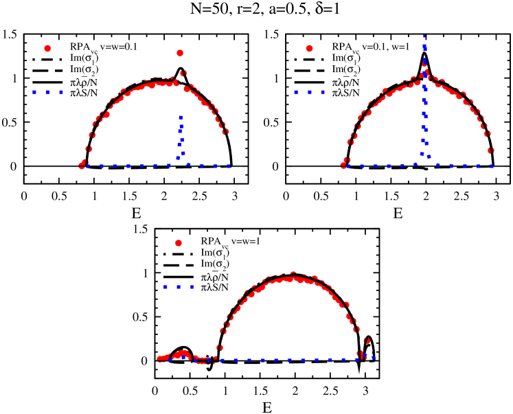
Figure 2: Same as Figure 1 but for $a=0.5$.

In Refs. [12, 13] we have given explicit analytical expressions for the location and the spreading width of the doorway state as functions of the parameters of the underlying dynamical model. In spite of determined efforts we have not been able to derive similarly useful expressions for the RPA approach. The reason is that in comparison to the shell-model case of Eq. (1), the matrix dimension of the RPA approach of Eq. (8) is doubled. In the shell-model case of Eq. (1), the Pastur equation is of second order and lends itself to a straightforward analytical treatment. In contradistinction, the Pastur equations (25) involve two functions $\sigma_{1}(E)$ and $\sigma_{2}(E)$ and are effectively of fourth order. Even within a perturbative treatment of the doorway state, the complexity of the resulting expressions for $\rho(E)$ and $S(E)$ is such that they do not elucidate the physical properties of the doorway state. For these reasons we confine ourselves to a presentation and discussion of the numerical results.

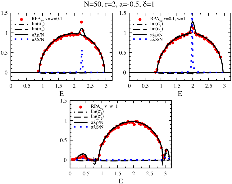
Figure 3: Same as Figure 1 but for $a=-0.5$.

The parameters of the variable-coupling model were chosen as follows. The location of the unperturbed background states was taken at $r=2$, see Eq. (4). The dimension of the random matrices $A$ and $C$ in Eq. (5) was $N=50$, the half width of the spectrum of the random matrix $A$ was chosen as $\lambda=1/2$, see Eqs. (6). These parameters were held fixed for all cases calculated. Without coupling to the doorway state and for $C=0$, the spectrum of $A$ extends from $E=1$ to $E=3$ and from $E=-3$ to $E=-1$. We have done calculations for several values of the parameter $a$ (the unperturbed location of the doorway state in Eq. (8)), $v$ and $w$ (strength of the coupling between the doorway state and the background states in Eq. (8)), and $\delta$ (relative strength of the random matrices $C$ and $A$ as defined in Eqs. (19)). In the figures shown we confine ourselves to values of $a$ such that the unperturbed position of the doorway state is within the spectrum of background states generated by $A$. Only the positive part of the energy spectrum is shown in all figures.

In the case of the numerical diagonalization of the RPA equations, the level density is calculated as number of states per bin. In order to limit statistical fluctuations, the bin width cannot be taken arbitrarily small and it turns out to be typically larger than the doorway state width. Hence, to make a meaningful comparison between the numerical diagonalization and the Pastur results, we have introduced a smoothed strength function $\bar{S}(E)$, obtained by convoluting the strength function (27) with a Gaussian distribution of variance equal to the bin width. For the purpose of comparison, in the figures we display the smoothed dimensionless total level density $\pi\lambda\bar{\rho}(E)/N$, with $\bar{\rho}$ defined as

$$\bar{\rho}(E)=-\frac{N}{\pi\lambda}\Im\big{(}\sigma_{1}(E)+\sigma_{2}(E)\big{)}+\bar{S}(E)\ ,$$ (28)

instead of $\rho$ as given in Eq. (26).

In the figures we also display the contributions due to $-\Im\sigma_{1}$ and $-\Im\sigma_{2}$ as defined in Eqs. (25) and to $\pi\lambda S(E)/N$ with $S(E)$ defined in Eq. (27) (i. e., the strength function as obtained from the Pastur equations). The result of the numerical diagonalization of the RPA equations is shown as red dots.

Figure 4: Same as Figure 1 but for changed values of the parameters as indicated.

The top left panel of Fig. 1, obtained for weak coupling, shows the expected pattern of a doorway state in the center of and superposed over the semicircular spectrum of background states. Due to the coupling matrix $C$ that spectrum is displaced toward the left from its original position for $C=0$. As the strength parameter $w$ is increased (second panel), the doorway state is shifted toward smaller energies. This reflects the increased attraction between states of positive and negative energy already observed in Ref. [15]. Such attraction is due to terms like $w$ or $C$ that connect the positive- and the negative-energy parts of the RPA matrix. Keeping the parameter $w$ fixed and increasing the parameter $v$ (third panel) causes level repulsion and shifts the doorway state outside the spectrum of background states. The same pattern is discernible in Figs. 2 and 3 where the original location of the doorway state is defined by $a=0.5$ and by $a=-0.5$, respectively. In all three figures there appear bumps at small energies for $v=w=1$. We have not investigated these more closely.

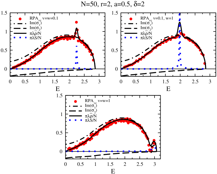
Figure 5: Same as Figure 1 but for changed values of the parameters as indicated.

Figures 4 and 5 show cases where the coupling $\delta$ between positive- and negative-energy states is increased to $\delta=2$. In that case, attraction between the two parts of the spectrum significantly shifts and distorts the semicircular spectrum of the background states, see Ref. [15]. For $a=0$ (Fig. 4) and weak coupling (top left panel) the doorway state is unaffected by this change. However, it completely loses its identity and disappears among the background states when either $w$ or both $v$ and $w$ are significantly increased. That is not the case for $a=0.5$ where the doorway state keeps its identity but moves in a manner similar to that of Figures 1 to 3. The difference is due to the contribution of the doorway state shown in Figures 4 and 5.

In Fig. 6 we display the strikingly different behavior of the doorway state strength function when the position $a$ of the collective state moves out of the background center. For $a=0$ the strength decreases when the coupling to the negative energy states is increased, whereas the opposite happens when the collective state is not centered. This behavior is the reason for the differences between the top right panels of Figures 4 and 5.

Finally, note that the doorway strength is of order $1/N$ with respect to the background (see Eq. (26)), so that for values of $N$ larger than the one employed in the figures ($N=50$) it would become progressively less visible, decreasing its heigth as $1/N$.

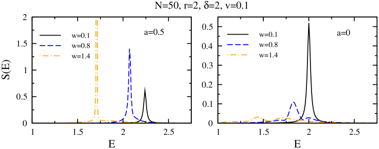
Figure 6: The evolution of the doorway strength function for two different state position varying the strength of the coupling.

5 Conclusions

In the framework of the RPA approximation we have investigated a doorway state coupled to a sea of $N$ background states. The latter are described in terms of the random-matrix model for the RPA equations developed and investigated in Ref. [15]. The symmetry of the RPA equations allows for two possibilities, strong coupling or variable coupling of the doorway state to the background states. We have shown that the first alternative is physically not interesting, and we have not considered it in the paper. For the second alternative we have in the limit $N\to\infty$ derived the Pastur equation for the average level density. That equation has twice the dimension of the standard case. In contrast to the standard situation, that makes it virtually impossible to obtain even approximate expressions for the location and width of the doorway state. Therefore, we have confined ourselves to a numerical approach. We have shown that the solution of the Pastur equation agrees well with the results of matrix diagonalization for $N=50$.

We have shown that the theoretical description of doorway states within the RPA framework is distinctly different from the standard treatment. The two interaction matrix elements $v$ and $w$ that characterize the interaction of the doorway state with the background states play very different roles. While $v$ couples the doorway state to states of the same (positive or negative) energy, $w$ couples the doorway state at positive energy to background states at negative energy and vice versa. The matrix element $v$ causes a spreading of the doorway state and the associated level repulsion, similar to the standard situation. The matrix element $w$ causes level attraction and moves the position of the doorway state rather strongly without discernibly affecting its width.

Acknowledgements. One of us (HAW) is grateful to the late O. Bohigas for discussions that sparked the present investigation.

Appendix: Failure of the Strong-Coupling Model

We show that in the strong-coupling model, the spreading width is of the order of the total width of the spectrum. To that end we display the doorway state in the matrix ${\cal H}$ explicitly. The separable matrix with elements $a_{\mu}a^{*}_{\nu}$ in Eq. (7) has a single non-vanishing eigenvalue $|a|^{2}$ and is diagonalized by a unitary matrix $U$ that obeys $\sum_{\nu}U_{\mu\nu}a_{\nu}=\delta_{\mu 1}a$. We use the transformation

$${\cal H} \to \left(\matrix{U&0\cr 0&U^{*}\cr}\right){\cal H}\left(\matrix{U^{\dagger}&0\cr 0&U^{T}\cr}\right)$$ (29)

$$= \left(\matrix{r\delta_{\mu\nu}&0\cr 0&-r\delta_{\mu\nu}\cr}\right)$$

$$+ \left(\matrix{|a|^{2}\delta_{\mu 1}\delta_{\nu 1}&a^{2}\delta_{\mu 1}\delta_{\rho(N+1)}\cr-(a^{*})^{2}\delta_{\sigma(N+1)}\delta_{\nu 1}&-|a|^{2}\delta_{\sigma(N+1)}\delta_{\rho(N+1)}\cr}\right)$$

$$+ \left(\matrix{(UAU^{\dagger})_{\mu\nu}&(UCU^{T})_{\mu\rho}\cr-(U^{*}C^{*}U^{\dagger})_{\sigma\nu}&-(U^{*}A^{*}U^{T})_{\sigma\rho}\cr}\right)\ .$$

Because of generalized unitary invariance, the transformed matrices $UAU^{\dagger}$ and $UCU^{T}$ belong to the same ensemble as the matrices $A$ and $C$, respectively, and we replace them by the latter without loss of generality. Then the sum of the first and the third terms on the right-hand side of Eq. (29) yields ${\cal H}^{(0)}$ in Eq. (3), and we have

$${\cal H}={\cal H}^{(0)}+\left(\matrix{|a|^{2}\delta_{\mu 1}\delta_{\nu 1}&a^{2}\delta_{\mu 1}\delta_{\rho(N+1)}\cr-(a^{*})^{2}\delta_{\sigma(N+1)}\delta_{\nu 1}&-|a|^{2}\delta_{\sigma(N+1)}\delta_{\rho(N+1)}\cr}\right)\ .$$ (30)

The strong-coupling model has four parameters, the three parameters $r,\lambda,\gamma$ of the stochastic model and the parameter $a$ that determines the position of the collective state. There is no independent parameter that would determine the strength of the coupling between the collective state and the background states. According to Eq. (30) that coupling is mediated by those matrix elements of $A$ and of $C$ that appear in the first and the $N+1$st rows and columns of ${\cal H}^{(0)}$. For a semiquantitative estimate we apply the standard expression $\Gamma^{\downarrow}=2\pi\langle|v|^{2}\rangle\rho(E)$ for the spreading width to our case. Here $\langle|v|^{2}\rangle$ is the mean square matrix element coupling the doorway state and the background states, and $\rho(E)$ is the average level density of the latter. In the present case we have $\langle|v|^{2}\rangle=\langle|A|^{2}_{11}\rangle=\lambda^{2}/N$ and, in the center of the GOE spectrum, $\rho(E)=N/(\pi\lambda)$. Thus, $\Gamma^{\downarrow}=2\lambda$ equals the width of the spectrum of the background states. That feature violates postulate (iv) of Section 1 and is totally unphysical. It implies that the resonance due to the doorway state cannot be distinguished from the spectrum of the background states: There simply is no identifiable doorway state. A more detailed investigation that takes account of the matrices $C$ via the Pastur equation does not modify that conclusion in any essential way since there is no mechanism to reduce the value of the spreading width by a factor $1/N$.

References

- [1] M. N. Harakeh and A. Wooude, Giant Resonances, Oxford University Press, Oxford, 2001.
- [2] N. Auerbach, J. Hüfner, A. F. Kerman, and C. M. Shakin, Rev. Mod. Phys. 44 (1972) 48.
- [3] M. A. Nielsen and I. L. Chuang, Quantumm Computation and Quantum Information, Cambridge University Press, Cambridge (2000).
- [4] T. Gorin, T. Prozen, T. H. Seligman, and M. Znidaric, Phys. Rep. 435 (2006) 33.
- [5] S. Aberg, T. Guhr, M. Miski-Oglu, and A. Richter, Phys. Rev. Lett. 100 (2008) 204101.
- [6] T. Ridley, J. T. Hennessy, R. J. Donovan, K. P. Lawley, S. Wang, P. Brint, and E. Lane, J. Phys. Chem. A 112 (2008) 7170.
- [7] P. Jaquod and C. Petitjean, Adv. Phys. 58 (2009) 67.
- [8] I. Shchatsinin, H.-H. Ritze, C. P. Schulz, and I. V. Hertel, Phys. Rev. A 79 (2009) 053414.
- [9] H. Kohler, H.-J. Sommers, S. Aberg, and T. Guhr, Phys. Rev. E 81 (2010) 050103(R).
- [10] H. Kohler, H.-J. Sommers, and S. Aberg, J. Math. Phys. A: Math. Theor. 43 (2010) 215102.
- [11] H. A. Weidenmüller and G. E., Mitchell, Rev. Mod. Phys. 81 (2009) 539.
- [12] A. De Pace, A. Molinari, and H. A. Weidenmüller, Ann. Phys. 322 (2007) 2446.
- [13] A. De Pace, A. Molinari, and H. A. Weidenmüller, Nucl. Phys. A 849 (2011) 15.
- [14] P. Ring and P. Schuck, The Nuclear Many-Body Problem, Springer-Verlag, Heidelberg, 1980.
- [15] X. Barillier-Pertuisel, O. Bohigas, and H. A. Weidenmüller, Ann. Phys. 324 (2009) 1855.
- [16] A. Altland and M. R. Zirnbauer, Phys. Rev. B 55 (1997) 1142.