A Darling-Erdős-type CUSUM-procedure
for functional data II

Abstract

This article considers testing for mean-level shifts in functional data. The class of the famous Darling-Erdős-type cumulative sums (CUSUM) procedures is extended to functional time series under short range dependence conditions which are satisfied by functional analogues of many popular time series models including the linear functional AR and the non-linear functional ARCH. We follow a data driven, projection-based approach where the lower-dimensional subspace is determined by (long run) functional principal components which are eigenfunctions of the long run covariance operator. This second-order structure is generally unknown and estimation is crucial - it plays an even more important role than in the classical univariate setup because it generates the finite-dimensional subspaces. We discuss suitable estimates and demonstrate empirically that altogether this change-point procedure performs well under moderate temporal dependence.

Moreover, Darling-Erdős-type change-point estimates based on (long run) functional principal components as well as the corresponding »fully-functional« counterparts are provided and the testing procedure is finally applied to publicly accessible electricity data from a German power company.

Keywords

Functional data analysis, Change-point test, Change-point estimates, $L^{\kappa}$-$m$-approximable time series, Darling-Erdős, Long run variance

AMS Subject Classification

62G05, 62G10, 62G20

Introduction

The interest and the research activities in »change-point analysis« for multivariate, high-dimensional and especially for functional data are enormous which is a consequence of the increasingly growing computational capacities. These activities are reflected by the amount and the high frequency of published works and in particular by survey articles that appeared recently. One of the fundamental and most studied problems in change-point analysis is concerned with a simple abrupt change in the mean - the »at most one change« (AMOC) model.

• We consider this problem in the functional setup, i.e. where each observation is a curve and the mean is a deterministic function.

• We want to know whether the overall shapes of the mean-curves have changed over time at some arbitrary time point or not.

Our investigations are based on the work of Berkes et al.​ (2009) who studied the same problem and introduced a (differently weighted) nonparametric CUSUM procedure for detection of changes in the mean of functional observations in the i.i.d. setting. Berkes et al.​ (2009) suggested an intuitive approach which essentially relies on a multivariate CUSUM by projecting the functional time series on a finite dimensional subspace which captures the dynamics of the data in a beneficial manner in order to obtain reasonable power. The authors proposed to select the subspace spanned by functional principal components (FPC’s), i.e. the eigenfunctions of the covariance operator. This approach is motivated by their well known optimality properties regarding dimension reduction (cf. Ramsay & Silverman (2005)). Since then, FPC’s - which play widely known an outstanding role in functional data analysis - have been successfully incorporated into many further functional »stability-testing« procedures under independence as well as more recently under dependence (cf. Horváth & Kokoszka (2012) for an overview and also Berkes et al.​ (2009), Hörmann & Kokoszka (2010) and Aston & Kirch (2012) in particular for the change in the mean setting). Later on, it was realized that long run FPC’s, given as eigenfunctions of the so-called long run covariance operator, are advantageous (cf. Horváth et al.​ (2013, 2014) and Torgovitski (2014)).

In this article we will stick to the latter approach. We pick up and continue the work of Torgovitski (2014) (cf. also Zhou (2011)) extending the results from the $m$-dependent setting to the more challenging and realistic models of weakly dependent time series with a focus on the framework of $L^{\kappa}$-$m$-approximability (cf., e.g., Hörmann & Kokoszka (2010) and Horváth et al.​ (2013)). As in Torgovitski (2014), the procedure will be based on the dimension-reduction approach of Berkes et al.​ (2009). To establish asymptotics we will incorporate several steps outlined in Torgovitski (2014) and combine them with results of Berkes et al.​ (2011, 2013), Horváth et al.​ (2013) and Aue et al.​ (2014).

This article contributes to the massive amount of recent works on change-point testing and estimation in functional (or generally high-dimensional) data and is a revised version of Torgovitski (2014b).

1. On one hand, our results on long run covariance operator estimation »complement« the findings of Hörmann & Kidziński (2015). Their results are slightly stronger but our proof technique is different and thus is of separate interest.

2. On the other hand, our results on the (multivariate) Darling-Erdős limit theorems complement the related discussion of Kamgaing & Kirch (2016). Here, we show additional conditions that emerge due to dimension reduction, i.e. due to the transition from the functional to the multivariate settings. Moreover, we verify conditions for the multivariate Darling-Erdős asymptotics explicitly under the specific dependence concept of $L^{\kappa}$-$m$-approximability.

3. Furthermore, we discuss the relation of projection-based and fully-functional estimates for change-points. This contributes to the investigation of some related estimates in the recent work of Aue et al.​ (2015).

4. Finally, we demonstrate the performance of the Darling-Erdős-type CUSUM procedure in Monte Carlo simulations and conduct an analysis of a real-life »electricity dataset«. Note that the »synthetic« simulations presented here and in the previous version Torgovitski (2014b) are used for comparison by Sharipov et al.​ (2015).

Notation 1.

In order to formalize the testing problem we have to introduce some notation first. We consider functional data $X(\cdot)$ as a random element on some probability space $(\Omega,{\cal A},P)$ with the state space $L^{2}[0,1]$. Throughout, let $L^{2}[0,1]$ denote the space of square-integrable functions with respect to the Lebesgue measure on $[0,1]$ equipped with the usual inner product and the corresponding norm, denoted by $\langle v,w\rangle=\int\!v(t)w(t)dt$ or $\|v\|$ for $v,w\in L^{2}[0,1]$, respectively. We also assume product measurability of $X(t)=X(t,\omega)$ with respect to $(t,\omega)\in[0,1]\times\Omega$. The mean of $X(\cdot)$ is defined as the unique function $\mu(\cdot)$, such that $\int\!x(t)\mu(t)dt=E\int\!x(t)X(t)dt$ holds true for all $x\in L^{2}[0,1]$ given that $E\|X\|<\infty$.

We assume that the observable sequence $\{X_{i}(\cdot)\}_{i\in\mathbb{Z}}$ consists of $L^{2}[0,1]$-valued random elements which are given by the functional »signal plus noise« model

$$X_{i}(t)=\mu_{i}(t)+Y_{i}(t),\qquad t\in[0,1],$$ (1.1)

with mean functions $\mu_{i}(\cdot)\in L^{2}[0,1]$ and with innovations fulfilling our basic (M), below. The dependence structure of the innovations will be specified later on. We want to test retrospectively the null hypothesis of no change in the mean, i.e.

$$H_{0}:\qquad \mu_{1}(\cdot)=\ldots=\mu_{n}(\cdot)$$

against the alternative of a change in the mean

$$H_{A}:\qquad \mu_{1}(\cdot)=\ldots=\mu_{\lfloor n\theta\rfloor}(\cdot)\neq\mu_{\lfloor n\theta\rfloor+1}(\cdot)=\ldots=\mu_{n}(\cdot)$$

at some unknown time point characterized by some (unknown) constant change parameter $\theta\in(0,1)$.

Assumption (M).

• The functional innovation sequence $\{Y_{i}\}_{i\in\mathbb{Z}}$ is centered and strictly stationary;

• $E\|Y_{1}\|^{\nu}<\infty$ for some $\nu>2$.

The structure of this article is as follows: In Section 2 we formulate the dependence concept of $L^{\kappa}$-$m$-approximability for our observations. In Section 3 we present the testing procedure together with the asymptotics under the null hypothesis and under the alternative. Section 4 focuses on estimation of long run FPC’s. The performance is finally demonstrated in Section 5 including an application example. All proofs are postponed to Section 6.

Weakly dependent time series

We consider the »mathematically convenient« concept of $L^{\kappa}$-$m$-approximable time series which is currently of major interest in univariate, multivariate and functional settings and covers many relevant time series models (cf., e.g., amongst many others Aue et al.​ (2009), Hörmann & Kokoszka (2010), Aston & Kirch (2012), Horváth et al.​ (2013, 2014), Jirak (2012, 2013), Berkes et al.​ (2013), Chochola et al.​ (2013) and Hörmann & Kidziński (2015)). Hörmann & Kokoszka (2010) and Berkes et al.​ (2011) contain extensive discussions and comparisons to other related dependence concepts.

We formulate the dependence concept in general real and separable Hilbert spaces $H$ but having the special cases $H=L^{2}[0,1]$ and $H=\mathbb{R}^{d}$ in mind. The reason for this is that we will use the notion of $L^{\kappa}$-$m$-approximability in both spaces because we will also deal with appropriate $\mathbb{R}^{d}$-valued approximations of the original $L^{2}[0,1]$ valued time series in our proofs. For a moment, let $\|\cdot\|_{H}$ denote a norm in the space $H$ and recall that $E(\|X\|_{H}^{\kappa})^{1/\kappa}$ is the $L^{\kappa}(\Omega,P)$-norm for the real-valued random variable $\|X\|_{H}$. Later on we will write $\|\cdot\|$ for the $L^{2}$ norm or $|\cdot|$ for the Euclidean norm, respectively.

Definition 2.1.

The $H$-valued sequence $\{Y_{i}\}_{i\in\mathbb{Z}}$, defined on some common probability space $(\Omega,{\cal A},P)$, is $L^{\kappa}$-$m$-approximable with rate $\delta(m)=o(1)$, $\delta(m)\geq 0$ and with $\kappa\geq 2$ iff $E[\|Y_{0}\|_{H}^{\kappa}]<\infty$ and the following conditions hold true:

• The $Y_{i}$’s admit a »Bernoulli shift« representation, i.e.

  $$Y_{i}=f(\ldots,\varepsilon_{i+1},\varepsilon_{i},\varepsilon_{i-1},\ldots),$$ (2.1)

  where the innovations $\varepsilon_{i}$ are i.i.d. $S$-valued random elements, $S$ is some measurable space and $f$ is a measurable mapping $f:S^{\infty}\rightarrow H$.

• The $Y_{i}$’s are approximated by $m$-dependent random variables in the sense that, as $m\rightarrow\infty$,

  $$E(\|Y_{0}-Y_{0}^{(m)}\|^{\kappa}_{H})^{1/\kappa}={\mathcal{O}}(\delta(m)),$$ (2.2)

  where $Y_{i}^{(m)}$ are $m$-dependent copies of $Y_{i}$ defined via

  $$Y^{(m)}_{i}=f(\ldots,\varepsilon^{(m,i)}_{i+M},\varepsilon_{i+(M-1)},\ldots,\varepsilon_{i},\ldots,\varepsilon_{i-(M-1)},\varepsilon^{(m,i)}_{i-M},\ldots)$$ (2.3)

  with $M=\max\{\lfloor m/2\rfloor,1\}$ for all integer $m\geq 0$ and where the family

  $$\{\varepsilon_{r},\varepsilon_{i}^{(k,j)},\;i,j,r,k\in\mathbb{Z},\;k\geq 0\}$$

  is i.i.d.

• If $\{Y_{i}\}$ is function-valued with $H=L^{2}[0,1]$ then $({\cal B}_{[0,1]}\otimes{\cal A})-{\cal B}_{\mathbb{R}}$ measurability is assumed.

Typical conditions on the rate $\delta(m)$ are summability $\sum_{m=1}^{\infty}\delta(m)<\infty$, polynomial decay $\delta(m)={\mathcal{O}}(m^{-\nu})$ for some $\nu>2$ or exponential decay $\delta(m)={\mathcal{O}}(\exp(-cm))$ with some $c>0$, where the latter is here the strongest condition but already satisfied for many models such as, e.g., the $H$-valued AR(1).

Remark 2.2.

We are interested in the causal case of $L^{\kappa}$-$m$-approximability, i.e. that $Y_{i}=f(\varepsilon_{i},\varepsilon_{i-1},\ldots)$ holds true. This is a special case of (2.1) but the two-sided »noncausal« representation (2.1) appears to be useful in the proofs, where we will deal with time-inversed $L^{\kappa}$-$m$-approximable time series $\{Y_{-i}\}_{i\in\mathbb{Z}}$. Therefore, observe that

$$Y_{-i}=f(\varepsilon_{-i},\varepsilon_{-(i+1)},\varepsilon_{-(i+2)},\ldots)$$

is noncausal but still $L^{\kappa}$-$m$-approximable according to the two-sided Definition 2.1, above.

Remark 2.3.

Note that some recent literature (e.g. Berkes et al.​ (2013) and Horváth et al.​ (2014)) works with a slightly modified condition (2.2) where the left-hand side of (2.2) is substituted by $\smash{E(\|Y_{0}-Y_{0}^{(m)}\|^{\kappa}_{H})^{1/\tilde{\kappa}}}$ with some $\tilde{\kappa}>\kappa$.

The testing procedure

For the sake of generality and clarity, the testing procedure will be described in a unifying functional framework where we separate and highlight those conditions which essentially allow us to derive suitable asymptotics without a priori specifying a particular time series model or a dependence concept. The conditions presented below in this section were (to some degree) implicitly contained in Torgovitski (2014). Here, the theoretical focus will be more on verification of all stated conditions for $L^{\kappa}$-$m$-approximable time series.

The CUSUM procedure, which will be presented below, belongs to the class of »FPC-based approaches« and utilizes the second-order structure of the time series for an appropriate data-driven subspace selection. As mentioned in the introduction, we will assume a functional time series $\{X_{i}\}$ with functional innovations $\{Y_{i}\}$ and work with long run FPC’s following, e.g., Horváth et al.​ (2013, 2014) and Torgovitski (2014). Those are eigenfunctions of the long run covariance operator ${\cal C}$ of $\{Y_{i}\}_{i\in\mathbb{Z}}$ which, given (M), can be formally defined as an integral operator

$$\big{(}{\cal C}x\big{)}(t)=\int{\!\zeta(t,s)x(s)}ds,$$

$t\in[0,1]$, $x\in L^{2}[0,1]$, $\int:=\int_{0}^{1}$ with kernel

$$\zeta(t,s)=\sum_{r\in\mathbb{Z}}E[Y_{0}(t)Y_{r}(s)].$$ (3.1)

This operator is well-defined if

$$\zeta\in L^{2}([0,1]\times[0,1])$$ (3.2)

holds true in which case it is symmetric Hilbert-Schmidt and positive. Hence, ${\cal C}$ can be written using the spectral decomposition as

$$({\cal C}x)(t)=\sum_{j=1}^{\infty}\lambda_{j}\Big{[}\int\!x(s)v_{j}(s)ds\Big{]}v_{j}(t),$$ (3.3)

$t\in[0,1]$, $x\in L^{2}[0,1]$, with real eigenvalues $\lambda_{1}\geq\lambda_{2}\geq\ldots\geq 0$ in descending order and corresponding orthonormal eigenfunctions $v_{1}(t),v_{2}(t),\ldots$. The convergence of the series (3.1) and (3.3) above is meant in the $L^{2}([0,1]\times[0,1])$ or $L^{2}[0,1]$ sense, respectively. Clearly, the eigenvalues are non-negative due to the positiveness of ${\cal C}$.

Remark 3.1.

Notice, that the decomposition (3.3) is obviously ambiguous. One reason are signs: each eigenvalue $\lambda_{j}$ is always associated at least with two eigenfunctions $v_{j}$ and $-v_{j}$; Another source of ambiguity is the geometric multiplicity of $\lambda_{j}$ being larger than one. The statistic will be constructed in such a way that it will turn out to be invariant under changes of signs. Also, conditions will be imposed (cf. (4.2) below) to ensure that relevant eigenspaces are only one-dimensional - both is standard practice for FPC-based statistics. (In the following we tacitly restrict ourselves to $\lambda_{d}>0$, i.e. the functional data is at least $d$-dimensional.)

For testing of $H_{0}$ against $H_{A}$ we will work with the following CUSUM statistic

$$\begin{split}T_{n}(X;v,\lambda)=\max_{1\leq k<n}w(k/n)\left(\frac{\eta^{2}_{k,1}}{\lambda_{1}}+\ldots+\frac{\eta^{2}_{k,d}}{\lambda_{d}}\right)^{1/2}\end{split}$$ (3.4)

with scores

$$\eta_{k,r}=\eta_{k,r}(X;v)=n^{-1/2}\int\!\sum_{i=1}^{k}[X_{i}(t)-\bar{X}_{n}(t)]v_{r}(t)dt$$

where $w(t)=(t(1-t))^{-1/2}$ is a suitable weight function related to the variance of a Brownian bridge and $d\in\mathbb{N}$ is a fixed positive integer specifying the dimension of the subspace chosen for projecting. Notice, that in (3.4) $X$, $v$ or $\lambda$ represent $\{X_{i}\}_{i\in\mathbb{N}}$, $\{v_{i}\}_{i\in\mathbb{N}}$ or $\{\lambda_{i}\}_{i\in\mathbb{N}}$, respectively. The right-hand side of (3.4) can also be written compactly using vector-notation as

$$T_{n}(X;v,\lambda)=\max_{1\leq k<n}w(k/n)|n^{-1/2}\sum_{i=1}^{k}(\mathbf{X}_{i}-\bar{\mathbf{X}}_{n})|_{\mathbf{\Sigma}},$$

with the norm $|\cdot|_{{\mathbf{\Sigma}}}=|{\mathbf{\Sigma}}^{-1/2}\cdot|$ and where ${\mathbf{\Sigma}}(\lambda)={\rm diag}(\lambda_{1},\ldots,\lambda_{d})$ is a proper standardization matrix (cf. Torgovitski (2014) and 3.2 below). This presentation emphasizes that our CUSUM is based on the multivariate »projected version« of the data (1.1), i.e. on

$$\mathbf{X}_{i}=\boldsymbol{\mu}_{i}+\mathbf{Y}_{i},$$ (3.5)

where the $r$-th components of these vectors are

• the data scores $\mathbf{X}_{i,r}=\int\!X_{i}(t)v_{r}(t)dt$,

• the innovation scores $\mathbf{Y}_{i,r}=\int\!Y_{i}(t)v_{r}(t)dt$

• and the projected means $\boldsymbol{\mu}_{i,r}=\int\!\mu_{i}(t)v_{r}(t)dt$

for $r=1,\ldots,d$, respectively.

Remark 3.2.

The matrix ${\mathbf{\Sigma}}(\lambda)$ is the long run covariance matrix of the projected time series $\{\mathbf{Y}_{i}\}_{i\in\mathbb{Z}}$ which can be seen utilizing the orthonormality of the eigenfunctions:

$$\sum_{k\in\mathbb{Z}}E[\mathbf{Y}_{0,i}\mathbf{Y}_{k,j}]=\int\!\left(\int\!\zeta(t,s)v_{j}(s)ds\right)v_{i}(t)dt=\lambda_{j}\delta_{i,j}.$$

The diagonality of ${\mathbf{\Sigma}}$ is hereby one of the main advantages of working with the long run covariance operator ${\cal C}$. Also, the existence of ${\mathbf{\Sigma}}$ is inherited from the existence of the functional counterpart ${\cal C}$.

In applications, especially in the functional setup, the covariance structure, e.g. in our case the covariance operator ${\cal C}$, will be rarely known. Hence, the associated quantities such as the eigenelements $\{v_{i}\}_{i\in\mathbb{N}}$ and $\{\lambda_{i}\}_{i\in\mathbb{N}}$, are therefore also usually unknown and have to be estimated. Therefore, let $\{\hat{v}_{i}\}_{i\in\mathbb{N}}$ be orthonormal functions which together with non-negative scalars $\{\hat{\lambda}_{i}\}_{i\in\mathbb{N}}$, $\hat{\lambda}_{1}\geq\hat{\lambda}_{2}\geq\ldots\geq 0$, denote some generic estimates which will be specified later on. Thus, instead of working with $T_{n}=T_{n}(X;v,\lambda)$ we will consider

$$\begin{split}\hat{T}_{n}&=T_{n}(X;\hat{v},\hat{\lambda})=\max_{1\leq k<n}w(k/n)\left(\frac{\hat{\eta}^{2}_{k,1}}{\hat{\lambda}_{1}}+\ldots+\frac{\hat{\eta}^{2}_{k,d}}{\hat{\lambda}_{d}}\right)^{1/2}\end{split}$$ (3.6)

with estimated scores

$$\hat{\eta}_{k,r}=\eta_{k,r}(X;\hat{v})=n^{-1/2}\int\!\sum_{i=1}^{k}[X_{i}(t)-\bar{X}_{n}(t)]\hat{v}_{r}(t)dt$$

having in mind that formally $\hat{T}_{n}=\infty$ if $\hat{\lambda}_{r}=0$ for some $1\leq r\leq d$. The vector notation in the estimated case is given by $\hat{T}_{n}=\max_{1\leq k<n}w(k/n)|n^{-1/2}\sum_{i=1}^{k}(\hat{\mathbf{X}}_{i}-\bar{\hat{\mathbf{X}}}_{n})|_{\hat{{\mathbf{\Sigma}}}}$ where each component of the projected time series $\{\hat{\mathbf{X}}_{i}\}$ is $\hat{\mathbf{X}}_{i,r}=\int\!X_{i}(t)\hat{v}_{r}(t)dt$ and where $\hat{{\mathbf{\Sigma}}}={\rm diag}(\hat{\lambda}_{1},\ldots,\hat{\lambda}_{d})$. A natural estimate for the change-point is given analogously to (3.4) and (3.6) through

$$\hat{k}(\hat{v},\hat{\lambda},d)=\operatorname*{arg\,max}_{1\leq k<n}w(k/n)\left(\frac{\hat{\eta}^{2}_{k,1}}{\hat{\lambda}_{1}}+\ldots+\frac{\hat{\eta}^{2}_{k,d}}{\hat{\lambda}_{d}}\right)^{1/2}.$$

We will discuss some related estimates in 3.9, below.

The following conditions (L), (P1), (P2), (A1), (A2) and (B1), (B2) are the main »building blocks« which allow us to prove the limiting distribution of $\hat{T}_{n}$ under the null hypothesis and consistency under the alternative. Recall that (M) is always tacitly assumed. We proceed with conditions under the null hypothesis where the first (L) states the availability of a multivariate Darling-Erdős-type limit theorem for $T_{n}$ which will be a cornerstone for our further considerations. (See Berkes et al.​ (2009), Hörmann & Kokoszka (2010) and Aston & Kirch (2012) for related CUSUM procedures based on multivariate functional central limit theorems.)

Assumption (L).

It holds that, as $n\rightarrow\infty$,

$$\lim_{n\rightarrow\infty}P\left(a(\log n)T_{n}(Y;v,\lambda)-b_{d}(\log n)\leq x\right)=\exp(-2\exp(-x))$$ (3.7)

for all $x\in\mathbb{R}$, where $a(t)=(2\log t)^{1/2}$ and $b_{d}(t)=2\log t+(d/2){\log\log t}-\log\Gamma(d/2)$ denote the well known normalizing functions.

In the i.i.d. setting (L) is immediately implied by Csörgő & Horváth (1997, Theorem 1.3.1) if (ii) of (M) and (3.2) holds true. For strictly stationary $m$-dependent sequences (L) follows analogously using strong invariance principles derived in Horváth et al.​ (1999) (cf. Torgovitski (2014)). Verification of (L) under $L^{\kappa}$-$m$-approximability will be carried out further below but has now to be based on strong approximations derived recently in Aue et al.​ (2014). Further conditions (e.g. of mixing-type) which ensure (3.7) are briefly discussed in Kamgaing & Kirch (2016).

Remark 3.3.

It is worth noting, that strictly stationary $m$-dependent sequences, as considered in Horváth et al.​ (1999) or in Torgovitski (2014), are generally either not $L^{\kappa}$-$m$-approximable or that the rate function is unknown. As pointed out by Berkes et al.​ (2011, Section 3.1), they do not necessarily possess representation (2.1).

The following conditions on maxima of weighted (backward) partial sums of the innovations together with the subsequent conditions on rates for $\{\hat{v}_{i}\}_{i\in\mathbb{N}}$ and $\{\hat{\lambda}_{i}\}_{i\in\mathbb{N}}$ will ensure a proper »interplay« between the functional data and the multivariate statistic $\hat{T}_{n}$.

Assumption (P1).

It holds that, as $n\rightarrow\infty$,

$$\max_{1\leq k<n}k^{-1/2}\|\sum_{i=1}^{k}Y_{i}\| ={\mathcal{O}}_{P}(g(n)),$$

$$\max_{1\leq k<n}k^{-1/2}\|\sum_{i=1}^{k}Y_{-i}\| ={\mathcal{O}}_{P}(g(n)),$$

where the rate function $g(n)$ will be specified later on.

Assumption (A1).

Under $H_{0}$ it holds that, as $n\rightarrow\infty$,

$$\max_{i=1,\ldots,d}|\hat{\lambda}_{i}-\lambda_{i}|=o_{P}((\log\log n)^{-1}).$$

Assumption (A2).

Under $H_{0}$ it holds that, as $n\rightarrow\infty$,

$$\max_{i=1,\ldots,d}|\hat{v}_{i}-s_{i}v_{i}|=o_{P}((\log\log n)^{-1/2}/g(n)),$$

where $s_{i}$’s are random with $s_{i}\in\{1,-1\}$ and the rate function $g(n)$ is the same as in (P1).

The random $s_{i}$’s are typical in the functional setup and show up essentially due to the non-uniqueness of eigenfunctions but apparently do not affect the statistic (3.4). As already indicated, above assumptions are sufficient to obtain the limiting distribution of $\hat{T}_{n}$ which is stated in the next proposition and allows us to obtain critical values.

Theorem 3.4.

Let Assumptions (3.2), (L), (P1), (A1), (A2) and $\lambda_{d}>0$ hold true. Then under $H_{0}$ it holds that, as $n\rightarrow\infty$,

$$\lim_{n\rightarrow\infty}P\left(a(\log n)\hat{T}_{n}-b_{d}(\log n)\leq x\right)=\exp(-2\exp(-x))$$ (3.8)

for all $x\in\mathbb{R}$.

Remark 3.5.

By considering the univariate analogue of (A2) we note that $g(n)=(\log\log n)^{1/2}$ is the best possible rate (cf., e.g. Csörgő & Horváth (1997, Theorem A.4.1) for the famous Darling-Erdős asymptotics for i.i.d. random variables) and if such a rate holds true in (P1), then the rates in (A1) and (A2) coincide and are both of order $o_{P}((\log\log n)^{-1})$. In this article we will discuss results that allow us »a mathematically convenient derivation« of logarithmic rates $g(n)$ which are slightly weaker than $(\log\log n)^{1/2}$ but more than sufficient for our »practical« purposes (cf. 3.11, 3.12 and 3.13).

Before proceeding with the verification of conditions (L) - (A2), we turn to the alternative and state the conditions which ensure that the procedure detects changes

$$\Delta(t)=\mu_{n}(t)-\mu_{1}(t)$$ (3.9)

with $\Delta\neq 0$ in $L^{2}[0,1]$ with probability tending to 1, as $n\rightarrow\infty$. Analogous to (P1), we need a bound on partial sums and conditions on estimates $\hat{\lambda}_{j}$ and $\hat{v}_{j}$.

Assumption (P2).

The weak law of large numbers holds true, i.e. it holds that $\|\sum_{i=1}^{n}Y_{i}\|=o_{P}(n)$ as $n\rightarrow\infty$.

Estimates $\hat{\lambda}_{j}$ appear in the denominator of (3.6) and therefore need to be bounded. Recall, that we tacitly assume that all estimates are non-negative and in a decreasing order.

Assumption (B1).

Under $H_{A}$ it holds that $\hat{\lambda}_{1}=o_{P}(n/(\log\log n))$ as $n\rightarrow\infty$.

Assumption (B2).

Under $H_{A}$ it holds that, as $n\rightarrow\infty$,

$$|\int{\!\Delta(t)\hat{v}_{r}(t)}dt|\stackrel{{\scriptstyle P}}{{\longrightarrow}}\xi,$$ (3.10)

for some $1\leq r\leq d$ and some $\xi>0$. The change-function $\Delta(t)$ is defined in (3.9).

In order to obtain consistency for the change estimate $\hat{k}$ we state a condition that extends Csörgő & Horváth (1997, Theorem 2.8.1, disp. (2.8.7)) to projection-based estimates in the functional framework.

Assumption (E1).

Under $H_{A}$ it holds that, as $n\rightarrow\infty$,

$$\frac{n}{g^{2}(n)}\left(\hat{\lambda}_{d}/\hat{\lambda}_{1}\right)\stackrel{{\scriptstyle P}}{{\longrightarrow}}\infty,$$ (3.11)

where the rate function $g(n)$ is the same as in (P1).

Note that $|\hat{\lambda}_{1}/\hat{\lambda}_{d}|$ is the condition number of $\hat{{\mathbf{\Sigma}}}$ with respect to the Euclidean norm. Hence, one possible interpretation is that (3.11) excludes ill-conditioned estimates.

Remark 3.6.

Condition (3.10) has an intuitive interpretation in terms of (3.5). Therefore, notice that the condition $\int\!\Delta(t)v_{r}(t)dt=0$ for all $1\leq r\leq d$ is equivalent to $\boldsymbol{\mu}_{1}=\ldots=\boldsymbol{\mu}_{n}$, i.e. there would be »asymptotically« no change in the projected times series $\{\mathbf{X}_{i}\}$. Hence, (3.10) means that the change $\Delta$ has to be »asymptotically visible« in the projected time series $\{\hat{\mathbf{X}}_{i}\}$ in (3.5).

The above conditions are sufficient to state the following consistency results.

Theorem 3.7.

Let Assumptions (3.2), (L), (P2), (B1), (B2) and $\lambda_{d}>0$ hold true. Then under $H_{A}$ it holds that, as $n\rightarrow\infty$,

$$(\log\log n)^{-1/2}\hat{T}_{n}\stackrel{{\scriptstyle P}}{{\longrightarrow}}\infty.$$ (3.12)

Theorem 3.8.

Let Assumptions (3.2), (P1), (B2), (E1) and $\lambda_{d}>0$ hold true. Then under $H_{A}$ it holds that, as $n\rightarrow\infty$,

$$\hat{k}(\hat{v},\hat{\lambda},d)/n\stackrel{{\scriptstyle P}}{{\longrightarrow}}\theta.$$ (3.13)

Remark 3.9 (Fully-functional estimates).

An obvious drawback of projection-based approaches are the assumptions on the eigenstructure and on the visibility of projected changes. These assumptions can be »relaxed« in two steps:

1. First, note that Theorem 3.8 may be immediately restated for the estimate

   $$\hat{k}(\hat{v},1,d):=\operatorname*{arg\,max}_{1\leq k<n}w(k/n)\left(\hat{\eta}^{2}_{k,1}+\ldots+\hat{\eta}^{2}_{k,d}\right)^{1/2}$$

   without any assumptions on the eigenvalue estimates, without requiring $\lambda_{d}>0$ and such that (E1) simplifies to $g^{2}(n)/n\rightarrow 0$. However, we still need the visibility of the projected changes of (B2).

2. One possibility to avoid this issue is shown recently by Aue et al.​ (2015) in a closely related context. They considered fully-functional estimates of the change point to overcome problems with »high-frequency« changes. Those changes are »difficult« to detect with the principal component approach since they require a large dimension $d$ to satisfy (B2). Working with large $d$’s in turn requires to estimate small eigenvalues $\lambda_{d}\approx 0$, i.e. the change point estimation becomes »unstable«. Hence, it is worth mentioning that relying only on (M) and on (P1) with $g^{2}(n)/n\rightarrow 0$ it is straightforward to show (3.13) for the fully-functional Darling-Erdős type estimate

   $$\hat{k}(\hat{v},1,\infty) :=\operatorname*{arg\,max}_{1\leq k<n}w(k/n)\lim_{d\rightarrow\infty}\left(\hat{\eta}^{2}_{k,1}+\ldots+\hat{\eta}^{2}_{k,d}\right)^{1/2}$$

   $$=\operatorname*{arg\,max}_{1\leq k<n}w(k/n)\big{\|}n^{-1/2}\sum_{i=1}^{k}(X_{i}-\bar{X}_{n})\big{\|}.$$

   This follows by going through the proof of Theorem 3.8 or of the underlying result in Csörgő & Horváth (1997, Theorem 2.8.1).

Theorem 3.7 and Theorem 3.8 rely on (B2). The latter is verified under $H_{A}$ typically via the relation

$$\Big{|}|\int\!\Delta(t)\hat{v}_{r}(t)dt|-|\int\!\Delta(t)w_{r}(t)dt|\Big{|}={\mathcal{O}}_{P}\big{(}\|\hat{v}_{r}-c_{r}w_{r}\|\big{)}=o_{P}(1)$$ (3.14)

on showing that $\|\hat{v}_{r}-c_{r}w_{r}\|=o_{P}(1)$ for appropriate $w_{1},\ldots w_{r}\in L^{2}[0,1]$ (where $c_{r}\in\{0,1\}$ are random) together with $\int\!\Delta(t)w_{r}(t)dt\neq 0$ for some $1\leq r\leq d$. In the i.i.d. setting natural estimates $\hat{v}_{r}$ are given by the functional empirical principal components (cf. Berkes et al.​ (2009)) and it is shown that they converge (up to signs) to eigenfunctions $w_{r}$ of a contaminated operator (cf. also Aston & Kirch (2012) and Torgovitski (2014)). Therefore, however, technical conditions on the eigenstructure of the contaminated operator together with the orthogonality condition $\int\!\Delta(t)w_{r}(t)dt\neq 0$ for some $1\leq r\leq d$ have to be additionally imposed. In our setup, estimates $\hat{v}_{r}$ can always be chosen such that $\int\!\Delta(t)w_{r}(t)dt\neq 0$ (and therefore (B2)) is fulfilled even with $r=1$ where $w_{1}=\Delta/\|\Delta\|$. This is stated in 4.3 and has been observed by Horváth et al.​ (2014) in a related context.

We turn to the verification of the conditions stated in Assumptions (L), (P1) and (P2) in case of $L^{\kappa}$-$m$-approximability as described in Section 2. Conditions of (A1) and (A2) as well as of (B1) and (B2) concerning estimation will be verified separately in the next section.

Theorem 3.10.

Let $\{Y_{i}\}_{i\in\mathbb{Z}}$ be causal and $L^{\kappa}$-$m$-approximable with $\kappa>2$ and a rate $\delta(m)=m^{-\gamma}$ for some $\gamma>2$. Then Assumptions (3.2), (L) and (P2) are fulfilled.

The next proposition applies the famous work of Móricz (1976) which, in combination with a result of Tómács and Líbor (2006), will allow us to establish (P1).

Proposition 3.11.

Assume that for some constant $\kappa>2$, it holds that, as $n\rightarrow\infty$,

$$\left[E\big{\|}\sum_{i=1}^{n}Y_{i}\big{\|}^{\kappa}\right]^{1/\kappa}={\mathcal{O}}(n^{1/2}).$$ (3.15)

Then, it holds that, as $n\rightarrow\infty$,

$$\max_{1\leq k\leq n}k^{-1/2}\big{\|}\sum_{i=1}^{k}Y_{i}\big{\|}={\mathcal{O}}_{P}((\log n)^{1/\kappa}).$$

Now, in order to verify (P1), it is sufficient to show (3.15) for $\{Y_{i}\}_{i\in\mathbb{Z}}$ and $\{Y_{-i}\}_{i\in\mathbb{Z}}$. For $L^{\kappa}$-$m$-approximable and causal time series, (3.15) follows from Berkes et al.​ (2013, Theorem 3.3) given that $\kappa\in(2,3)$. In this article we verify (3.15) for $L^{\kappa}$-$m$-approximable noncausal time series based directly on Berkes et al.​ (2011, Proposition 4).

Proposition 3.12.

Let $\{Y_{i}\}_{i\in\mathbb{Z}}$ be $L^{\kappa}$-$m$-approximable (not necessarily causal) with $\kappa\in[2,3)$ and $\sum_{m=1}^{\infty}\delta(m)<\infty$. Then, as $n\rightarrow\infty$, it holds that

$$\left[E\big{\|}\sum_{i=1}^{n}Y_{i}\big{\|}^{\kappa}\right]^{1/\kappa}={\mathcal{O}}(n^{1/2}).$$

A combination of 3.11 and 3.12 immediately yields the following result.

Corollary 3.13.

Let $\{Y_{i}\}_{i\in\mathbb{Z}}$ be $L^{\kappa}$-$m$-approximable with $\kappa>2$ and causal with $\sum_{m=1}^{\infty}\delta(m)<\infty$, then (P1) is fulfilled with rate $g(n)=(\log n)^{1/2}$.

Altogether, Theorem 3.10 and 3.13 verify conditions (3.2), (L), (P1) and (P2) under $L^{\kappa}$-$m$-approximability with $\delta(m)={\mathcal{O}}(m^{-\gamma})$ for $\gamma>2$. The remaining Assumptions (A1), (A2), (B1) and (B2) ensure the validity of (3.8) and of (3.13), in view of Theorem 3.4 and Theorem 3.7. All these assumptions can be verified using suitable estimates which will be shown in the next section.

Estimation of the eigenstructure

In this section we discuss suitable estimates $\{\hat{v}_{i}\}$ and $\{\hat{\lambda}_{i}\}$ for $\{v_{i}\}$ and $\{\lambda_{i}\}$ which, as pointed out by Horváth et al.​ (2013), is an intricate problem. One possibility to obtain such estimates, suggested by the latter, is to consider the eigenstructure of Bartlett-type estimators $\hat{{\cal C}}$ for ${\cal C}$ of the following general form

$$\big{(}\hat{{\cal C}}x\big{)}(t)=\int{\!\hat{\zeta}(t,s)x(s)}ds,$$

where $x\in L^{2}[0,1]$, $t\in[0,1]$. The kernel $\hat{\zeta}$ is given by

$$\hat{\zeta}(t,s)=\sum_{r=-n}^{n}K(r/h_{n})\hat{\zeta}_{r}(t,s),\qquad t,s\in[0,1],$$ (4.1)

with covariance estimators

$$\hat{\zeta}_{r}(t,s)=\begin{cases}\frac{1}{n}\sum_{i=1}^{n-r}\left(X_{i}(t)-\bar{X}_{n}(t)\right)\left(X_{i+r}(s)-\bar{X}_{n}(s)\right),&r\geq 0,\\ \hat{\zeta}_{-r}(s,t),&r<0,\end{cases}$$

a symmetric, bounded and compactly supported kernel function $K(x)$ with $K(0)=1$ and a bandwidth $h_{n}\rightarrow\infty$ fulfilling $h_{n}=o(n)$. (Notice that, due to the compact support of $K(x)$, the summation in (4.1) is only up to $\lfloor ch_{n}\rfloor$ for some $c>0$.) These estimates were explored by Horváth et al.​ (2013) under $L^{\kappa}$-$m$-approximability in the context of a related two-sample problem.

We restrict ourselves now to the framework of $L^{\kappa}$-$m$-approximable time series. For the sake of simplicity we consider exponential decay rates $\delta(m)=\exp(-cm)$, $c>0$. This is not very restrictive and already covers important time series models, in particular the functional AR($p$) time series, and will be sufficient for our purposes. Notice that $\hat{{\cal C}}$ is symmetric Hilbert-Schmidt, hence has a spectral decomposition

$$(\hat{{\cal C}}x)(t)=\sum_{j=1}^{\infty}\hat{\lambda}_{j}\Big{[}\int\!x(s)\hat{v}_{j}(s)ds\Big{]}\hat{v}_{j}(t)$$

with real eigenvalues $\hat{\lambda}_{1}\geq\hat{\lambda}_{2}\geq\ldots$ and corresponding orthonormal eigenfunctions $\hat{v}_{1}(t),\hat{v}_{2}(t),\ldots$. Generally, the estimates of the eigenvalues may be negative but (at least under $H_{0}$) become eventually positive as $n\rightarrow\infty$. Subsequently, we use the same notation for the eigenstructure as used for generic estimates before. This should not lead to any confusion.

The following Theorem 4.1 is an extension of Theorem 2 of Horváth et al.​ (2013), where consistency has been shown (under weaker assumptions). We consider the case of $L^{4}$-$m$-approximable time series which allows us to work with the variances of the estimates.

Theorem 4.1.

Let $\{Y_{i}\}_{i\in\mathbb{Z}}$ be $L^{4}$-$m$-approximable with $\delta(m)=\exp(-cm)$, $c>0$, and not necessarily causal. Assume that, as $x\rightarrow 0$,

$$|K(x)-1|={\mathcal{O}}(x^{\rho})$$

for some $\rho\geq 1$. Then under $H_{0}$, it holds that, $\|\hat{\zeta}-\zeta\|={\mathcal{O}}_{P}((h_{n}/n)^{1/2}h_{n}+1/h_{n}^{\rho})$, as $n\rightarrow\infty$, using a bandwidth $h_{n}=\lfloor c^{\prime}n^{1/\gamma}\rfloor$ with some $\gamma>3$ and $c^{\prime}>0$.

As one would expect, the rate of convergence in Theorem 4.1 reflects that a higher smoothness of the kernel $K(x)$ at $x=0$ reduces the contribution of the »bias«. Admissible values for the »smoothness parameter« $\rho$ are, e.g.,

• $\rho=1$ for the Bartlett kernel $K(x)=(1-|x|)1_{[-1,1]}(x)$,

• $\rho=2$ for the Parzen kernel

• and arbitrary large $\rho$ for the flat-top kernels.

The main implication of this Theorem 4.1 for us is that a polynomial rate $\|\hat{\zeta}-\zeta\|$$=\smash{O_{P}(n^{-\varepsilon})}$ holds true for some $\varepsilon>0$. This allows a convenient verification of (A1) and (A2) via 3.13 together with Lemmas 2.2 and 2.3 of Horváth & Kokoszka (2012). For (A2) we have to assume additionally, as common in the functional setup, that the first $d$ eigenvalues of ${\cal C}$ are simple, i.e. that

$$\lambda_{1}>\lambda_{2}>\ldots>\lambda_{d}>\lambda_{d+1}$$ (4.2)

holds true. Hence, decomposition (3.3) is unique up to signs.

Proposition 4.2.

Under $H_{0}$ and the assumptions of Theorem 4.1 the (A1) holds true. If additionally (4.2) is assumed, then (A2) also holds true.

We conclude this section by an observation, which follows in view of (3.14) and due to the Lemma B.2 of Horváth et al.​ (2014) (cf. also (3.5) and (3.6) therein).

Proposition 4.3.

Let $\{Y_{i}\}_{i\in\mathbb{Z}}$ be $L^{4}$-$m$-approximable and causal. Under $H_{A}$ and the assumptions of Theorem 4.1 the (B1) and (B2) hold true.

As already mentioned in 2.3 the dependence condition in Horváth et al.​ (2014, disp. (2.4)) is slightly different. However, Lemma B.2 can be restated under our conditions due to Jirak (2013, Theorem 1.2).

Simulations

Monte Carlo simulation

We proceed with a Monte Carlo simulation of the finite sample behavior. In order to describe our setting and implementation details we recall that $X_{i}(t)=\mu_{i}(t)+Y_{i}(t)$.

Simulation setup:

The signal $\mu_{i}$ is set to $\mu_{i}(t)\equiv 0$ for $i=1,\ldots,n$ under the null hypothesis and

$$\mu_{i}(t)=\begin{cases}0,&i=1,\ldots,\lfloor n/2\rfloor,\\ \sin(t),&i=\lfloor n/2\rfloor+1,\ldots,n\end{cases}$$ (5.1)

under the alternative. The innovations follow the formal functional AR($1$) model

$$Y_{i}(t)=\int\!\Psi(t,s)Y_{i-1}(s)ds+\varepsilon_{i}(t),$$ (5.2)

for $t\in[0,1]$ and $i\in\mathbb{Z}$, where the shocks $\{\varepsilon_{i}\}$ are assumed to be Gaussian. Under the assumption of $\|\Psi\|<1$ this equation is known to have a unique $L^{\kappa}$-$m$-approximable solution where $\kappa\geq 2$ is arbitrary (due to Gaussianity of $\varepsilon_{i}$’s) and where the decay rate $\delta(m)$ is exponential according to Hörmann & Kokoszka (2010). We will analyze the performance using two different kernels

$$\Psi_{G}(t,s)=C_{G}\exp((t^{2}+s^{2})/2),\qquad\Psi_{W}(t,s)=C_{W}\min(t,s)$$

normalized by constants $C_{G},C_{W}\geq 0$, such that $\|\Psi\|=\psi$ for a prescribed value $\psi\in[0,1)$. These kernels are common benchmarks in the functional data change-point literature where $\Psi_{G}$ and $\Psi_{W}$ are usually referred to as »Gaussian« or »Wiener« kernels, respectively (cf. Horváth & Kokoszka (2012)).

Implementation details:

We have implemented the procedure in R using the »fda-package«. The shocks $\varepsilon_{i}(\cdot)$ are generated as paths of Brownian bridges on $[0,1]$ and are represented as functional objects via the fda-function Data2fd(...) by using a »$B$-Spline basis« of 25 functions. The same basis is also used to represent the kernel $\Psi$ and the innovations $Y_{i}(\cdot)$. More precise, the bivariate function $\Psi(t,s)$ is discretized on an equidistant grid $0=t_{1}<t_{2}<\ldots<t_{T}=1$ and for each $k=1,\ldots,T$ the univariate function $\Psi(t_{k},\cdot)$ is then represented as a functional object. Next,

$$I_{i}(t_{k})=\int\!\Psi(t_{k},s)Y_{i-1}(s)ds$$

are computed for all $k=1,\ldots,T$ and $I_{i}(\cdot)$ itself is represented as a functional object with domain $[0,1]$, again, using the same $B$-Spline basis as in the previous steps. Having computed $I_{i}$ we are in the position to add up $Y_{i}(\cdot)=I_{i}(\cdot)+\varepsilon_{i}(\cdot)$. The correct representation of the dependence structure is ensured by using a so-called »burn-in period« of length $N_{B}=100$, i.e. $Y_{1},\ldots Y_{n}$ are generated iteratively according to (5.2) beginning with $Y_{-{N_{B}}+1}:=\varepsilon_{-{N_{B}}+1}$ where, finally, the first $N_{B}$ observations $Y_{-{N_{B}}+1},\ldots,Y_{0}$ are discarded. The desired observations $X_{1},\ldots X_{n}$ are then created according to the signal plus noise representation $X_{i}=\mu_{i}+Y_{i}$ via (5.1).

The computation of the long run covariance estimator is carried out following Horváth et al.​ (2011) by using 25 orthonormal »Fourier basis« functions. For simplicity we make use of a plain kernel $K(x)=1_{[-1,1]}(x)$, which yields satisfactory results. The overall picture remains comparable if one chooses e.g. a flat-top kernel as in Horváth et al.​ (2013, disp. (4.1)) or a Bartlett kernel, instead.

Critical values:

The convergence in (3.8) is rather slow. For that reason, we follow the idea investigated by Csörgő & Horváth (1997), also successfully applied in a functional setting by Torgovitski (2014), by using quantiles of

$$V_{n}=\sup_{t\in I_{n}}\frac{|\mathbf{B}^{d}(t)|}{(t(1-t))^{1/2}},$$ (5.3)

where $\{\mathbf{B}^{d}(t),0\leq t\leq 1\}$ is a $d$-dimensional Gaussian process with components given by independent standard Brownian bridges $\{B_{i}(t),0\leq t\leq 1\}$ and e.g.  $I_{n}=[h_{n},1-h_{n}]$ with $h_{n}=(\log n)^{3/2}/n$. Asymptotic correctness of this choice follows from (3.8) (cf. Csörgő & Horváth (1997, Corollary 1.3.1) and the proof of Torgovitski (2014, Corollary 4.3)). An essential advantage of (5.3) is that quantiles can be computed using the expansion

$$P\left(V_{n}\geq x\right)=\frac{x^{d}\exp(-x^{2}/2)}{2^{d/2}\Gamma(d/2)}\left\{\left(1-\frac{d}{x^{2}}\right)\log\frac{(1-h_{n})^{2}}{h_{n}^{2}}+\frac{4}{x^{2}}+{\mathcal{O}}(x^{-4})\right\}.$$ (5.4)

This representation is well known as »Vostrikova’s tail approximation« (see Vostrikova (1981, disp. (18)) and also Csörgő & Horváth (1997, disp. (1.3.26))).

Dimension and bandwidth selection:

Parameters $d$ and $h=h_{n}$ remain to be specified where especially the selection of $h$ is known to be a complex problem in practice. For example $d$ can be chosen according to the generalized CPV-Criterion (cf. Section 4.1 of Horváth et al.​ (2014)) and $h$ could be specified (in appropriate cases) guided by rules from scalar time series as demonstrated by Hörmann & Kokoszka (2010). However, both issues are not the focus of our research and therefore an overview for a range of parameters is presented in the tables below.

Brief summary of simulations:

The behavior under $H_{0}$ or under $H_{A}$, respectively, is demonstrated in Table 1 - Table 4 (based on 1000 repetitions). For moderate dependence and moderate sample sizes the procedure performs rather well and comparable for both kernels $\Psi_{W}$, $\Psi_{G}$. Moreover, it shows overall robustness with respect to the selection of various (small) dimensions $d$ and bandwidths $h$. With increasing sample size the »bias« due to the dependencies fades out which is in accordance with the nonparametric nature of the procedure.

Table 1: Empirical sizes for functional AR(1) with Gaussian kernel $\Psi_{G}$; nominal level of $10\%$.

$n$	$\|\Psi_{G}\|$	$\bf{d}$	1	2	3	4	5		1	2	3	4	5
			$h=1$						$h=2$
50	0.1		7.2	6.9	5.1	3.4	3.9		9.9	6.7	4.9	5.1	5.2
	0.2		8.7	6.2	4.3	3.6	2.6		8.2	6.5	5.9	6.2	5.8
	0.4		8.7	5.3	3.4	3.9	2.3		7.0	5.8	5.3	5.3	5.7
	0.6		8.9	5.2	3.2	2.8	2.3		4.7	2.3	3.1	3.2	4.0
	0.8		11.8	7.9	4.7	2.9	2.9		6.4	3.1	3.0	3.1	3.8
100	0.1		11.5	10.1	9.7	8.6	6.5		9.8	9.4	7.9	6.1	5.9
	0.2		7.8	7.0	5.5	5.4	4.6		9.0	7.3	6.0	5.1	4.8
	0.4		9.3	6.8	5.6	5.9	4.9		6.7	4.6	5.1	3.8	3.3
	0.6		14.6	9.3	8.8	6.1	4.8		6.7	4.9	3.9	4.5	4.0
	0.8		16.1	11.1	8.2	7.0	5.2		7.1	6.0	4.6	4.1	3.5
300	0.1		10.8	10.5	12.1	10.8	9.6		11.1	9.3	7.6	6.9	7.8
	0.2		9.6	10.1	8.9	8.5	8.2		9.0	9.8	8.0	7.7	7.0
	0.4		10.9	10.0	9.5	9.6	9.3		9.7	10.9	8.5	7.8	8.5
	0.6		14.4	12.0	9.1	8.4	8.2		7.4	6.9	6.4	6.5	6.7
	0.8		20.2	15.2	12.9	12.8	9.8		10.1	8.8	7.9	8.1	7.4
500	0.1		10.8	9.3	9.4	9.0	8.9		10.1	8.8	8.3	7.9	9.1
	0.2		9.7	9.1	9.0	9.7	9.6		8.1	8.3	6.8	6.4	7.1
	0.4		11.7	11.2	10.8	10.2	10.1		9.5	9.5	9.9	9.0	8.4
	0.6		15.5	12.7	11.1	11.3	10.2		10.3	9.2	8.3	7.8	7.8
	0.8		20.6	18.1	15.6	14.1	13.0		12.4	9.1	10.3	9.1	8.3
			$h=3$						$h=4$
50	0.1		10.0	8.3	7.2	8.1	8.5		9.7	8.0	9.7	11.3	11.9
	0.2		9.1	6.3	7.1	7.2	8.3		9.3	7.3	8.7	9.1	10.2
	0.4		6.5	4.0	5.1	6.6	8.4		7.2	6.1	6.6	7.4	10.1
	0.6		4.8	3.4	3.1	3.4	3.7		5.9	5.3	5.8	6.8	9.5
	0.8		2.7	2.3	2.3	2.5	4.9		4.3	4.1	5.0	5.8	8.3
100	0.1		9.8	7.1	6.3	6.2	6.1		9.2	8.1	6.6	6.1	7.0
	0.2		8.7	7.9	7.4	7.6	7.4		9.3	8.4	7.3	7.5	7.6
	0.4		8.2	5.5	5.0	5.7	5.9		6.7	5.3	6.7	6.1	7.7
	0.6		5.5	3.7	4.1	3.9	4.3		7.1	5.7	5.0	4.5	5.0
	0.8		5.9	3.8	3.6	3.5	5.6		4.1	3.0	3.4	4.1	4.8
300	0.1		9.5	10.6	9.7	8.3	8.6		10.6	10.0	10.6	9.2	7.5
	0.2		7.5	10.0	9.7	9.0	8.5		8.5	7.9	8.3	8.2	7.5
	0.4		8.5	7.3	6.6	5.3	5.4		9.1	10.0	9.1	7.6	6.7
	0.6		6.9	6.8	7.3	6.5	6.8		8.5	7.1	7.6	6.5	5.3
	0.8		6.7	7.8	7.7	6.9	7.1		6.7	4.7	7.4	6.5	6.1
500	0.1		11.6	9.8	7.7	8.5	8.8		10.3	10.7	9.3	9.2	8.1
	0.2		9.5	8.7	7.5	8.1	6.7		9.9	9.7	8.1	7.9	8.5
	0.4		7.9	7.9	7.0	6.3	7.7		7.2	8.6	8.6	8.2	7.9
	0.6		7.4	6.7	7.7	7.5	7.4		8.6	7.1	6.7	6.8	6.5
	0.8		7.2	6.4	7.2	6.0	7.1		7.3	7.9	7.7	6.9	5.9

Table 2: Empirical sizes for functional AR(1) with Wiener kernel $\Psi_{W}$; nominal level of $10\%$.

$n$	$\|\Psi_{W}\|$	$\bf{d}$	1	2	3	4	5		1	2	3	4	5
			$h=1$						$h=2$
50	0.1		9.6	7.6	4.6	3.9	2.9		10.1	8.0	6.8	6.4	5.9
	0.2		9.8	5.9	4.6	2.8	2.8		8.0	4.4	4.0	4.8	5.1
	0.4		9.9	5.7	3.8	2.9	2.3		5.2	3.5	2.8	2.4	3.1
	0.6		11.2	5.2	2.7	2.1	1.8		4.8	3.3	2.5	2.7	3.2
	0.8		20.6	11.0	4.8	3.0	2.5		3.8	1.9	1.4	2.1	2.1
100	0.1		8.6	8.1	6.5	6.7	6.5		9.0	8.7	6.6	7.1	6.0
	0.2		8.8	8.0	7.9	6.0	5.8		8.5	6.7	6.1	5.1	4.9
	0.4		10.6	8.6	6.1	5.1	5.0		5.7	7.1	4.5	4.4	2.9
	0.6		13.9	10.3	7.4	4.8	3.9		6.0	4.6	3.2	2.8	2.7
	0.8		28.6	19.6	13.6	9.7	7.5		11.5	7.0	6.1	4.1	3.3
300	0.1		10.5	9.4	9.1	8.7	7.3		10.5	9.9	9.0	6.8	7.0
	0.2		9.6	10.3	10.0	8.5	8.9		9.2	8.5	8.3	7.6	7.2
	0.4		10.3	9.8	10.0	8.5	6.9		7.0	6.9	7.3	5.7	5.7
	0.6		19.1	15.5	12.7	9.9	8.5		8.9	8.2	7.7	6.4	6.0
	0.8		33.4	25.5	20.7	18.6	15.4		15.7	12.5	10.5	9.7	7.6
500	0.1		12.5	10.2	9.0	8.6	8.6		10.8	10.5	10.3	9.3	9.4
	0.2		10.8	10.0	8.9	10.1	8.4		9.5	8.8	8.3	7.4	6.9
	0.4		13.7	13.3	11.3	9.9	8.9		9.3	8.5	9.3	8.4	7.9
	0.6		18.2	14.3	12.8	11.7	10.9		11.4	9.5	7.9	7.5	8.6
	0.8		37.9	29.0	22.4	19.1	16.7		17.9	12.7	9.9	9.9	8.7
			$h=3$						$h=4$
50	0.1		10.5	7.6	8.2	7.9	7.9		8.4	8.3	8.9	10.3	12.3
	0.2		9.2	7.8	6.4	6.4	7.5		10.2	8.0	9.0	9.9	10.2
	0.4		5.5	4.4	3.9	6.3	5.7		6.0	6.2	6.0	8.1	9.2
	0.6		4.0	2.8	3.5	4.1	3.9		3.4	4.2	5.2	5.0	6.1
	0.8		1.9	3.3	3.1	3.9	3.4		2.4	2.8	3.1	3.5	5.4
100	0.1		9.3	8.3	7.7	6.7	7.1		10.9	6.9	7.5	7.8	9.3
	0.2		9.0	5.5	5.4	4.9	5.5		8.5	6.5	6.6	6.2	7.0
	0.4		7.3	4.1	4.0	3.9	4.5		7.2	4.9	5.3	5.8	6.3
	0.6		5.5	4.3	4.1	4.1	4.0		5.1	3.4	3.3	4.2	4.8
	0.8		5.8	3.9	3.1	3.3	3.2		2.8	3.3	2.9	4.3	4.7
300	0.1		9.7	8.4	7.4	6.5	6.2		9.2	9.0	7.5	6.8	6.8
	0.2		9.3	9.1	7.9	6.8	6.9		10.1	9.1	8.2	7.1	6.4
	0.4		7.7	8.1	5.7	5.8	5.0		7.2	8.3	6.7	6.7	7.0
	0.6		8.9	7.0	6.4	6.6	5.7		6.2	5.4	5.7	4.8	5.8
	0.8		9.7	7.7	7.1	7.1	6.1		6.2	7.3	4.7	6.0	5.5
500	0.1		10.8	9.8	7.7	8.4	8.0		9.6	8.6	9.7	8.5	7.5
	0.2		7.4	8.4	7.0	6.8	5.9		7.8	8.6	7.0	8.4	8.8
	0.4		9.8	8.9	7.2	7.1	6.5		6.3	7.9	7.6	8.7	8.0
	0.6		9.1	8.1	6.3	5.7	5.7		6.7	6.9	8.8	7.4	6.4
	0.8		10.7	8.8	7.3	7.9	7.4		8.5	7.8	7.3	7.0	7.6

Table 3: Empirical power for functional AR(1) with Gaussian kernel $\Psi_{G}$; $\mu_{1}\equiv 0$ and $\mu_{n}(t)=\sin(t)$; nominal level of $10\%$.

$n$	$\|\Psi_{G}\|$	$\bf{d}$	1	2	3	4	5		1	2	3	4	5
			$h=1$						$h=2$
50	0.1		99.4	99.9	99.9	99.1	52.4		95.2	40.8	3.3	4.0	4.0
	0.2		99.3	99.8	99.8	98.6	52.1		91.8	37.5	2.0	2.2	3.0
	0.4		94.8	99.7	99.1	96.2	45.0		83.0	28.5	1.5	1.8	2.8
	0.6		89.3	98.7	98.9	94.7	40.6		68.5	23.0	1.8	1.7	2.2
	0.8		81.1	97.6	96.1	91.2	38.7		54.0	18.9	0.6	0.7	1.7
100	0.1		100	100	100	100	100		100	100	100	100	100
	0.2		100	100	100	100	100		100	100	100	100	100
	0.4		100	100	100	100	100		100	100	100	100	100
	0.6		99.7	100	100	100	100		99.5	100	100	100	100
	0.8		98.7	100	100	100	100		95.4	100	100	100	100
300	0.1		100	100	100	100	100		100	100	100	100	100
	0.2		100	100	100	100	100		100	100	100	100	100
	0.4		100	100	100	100	100		100	100	100	100	100
	0.6		100	100	100	100	100		100	100	100	100	100
	0.8		100	100	100	100	100		100	100	100	100	100
500	0.1		100	100	100	100	100		100	100	100	100	100
	0.2		100	100	100	100	100		100	100	100	100	100
	0.4		100	100	100	100	100		100	100	100	100	100
	0.6		100	100	100	100	100		100	100	100	100	100
	0.8		100	100	100	100	100		100	100	100	100	100
			$h=3$						$h=4$
50	0.1		45.3	1.9	2.8	4.2	5.3		1.1	2.2	2.7	4.5	6.3
	0.2		37.4	2.1	2.7	3.7	4.3		1.2	2.3	4.0	4.4	6.5
	0.4		28.2	1.9	2.8	3.8	5.3		1.1	2.7	3.9	4.2	7.2
	0.6		15.8	1.0	2.0	3.0	3.7		0.4	1.6	2.4	4.3	5.5
	0.8		9.7	0.7	1.0	2.0	3.4		1.0	1.2	2.9	4.3	5.8
100	0.1		100	100	100	13.6	3.8		99.9	93.2	2.2	3.0	2.8
	0.2		100	100	99.1	12.7	4.6		99.9	91.6	2.3	3.0	3.7
	0.4		99.9	100	98.9	9.3	2.9		99.3	86.5	2.5	3.4	3.9
	0.6		99.0	100	97.6	8.9	1.9		93.8	81.0	2.8	3.9	4.1
	0.8		91.5	99.7	95.8	8.9	2.6		82.1	72.3	0.6	2.2	2.2
300	0.1		100	100	100	100	100		100	100	100	100	100
	0.2		100	100	100	100	100		100	100	100	100	100
	0.4		100	100	100	100	100		100	100	100	100	100
	0.6		100	100	100	100	100		100	100	100	100	100
	0.8		100	100	100	100	100		100	100	100	100	100
500	0.1		100	100	100	100	100		100	100	100	100	100
	0.2		100	100	100	100	100		100	100	100	100	100
	0.4		100	100	100	100	100		100	100	100	100	100
	0.6		100	100	100	100	100		100	100	100	100	100
	0.8		100	100	100	100	100		100	100	100	100	100

Table 4: Empirical power for functional AR(1) with Wiener kernel $\Psi_{W}$; $\mu_{1}\equiv 0$ and $\mu_{n}(t)=\sin(t)$; nominal level of $10\%$.

$n$	$\|\Psi_{W}\|$	$\bf{d}$	1	2	3	4	5		1	2	3	4	5
			$h=1$						$h=2$
50	0.1		99.0	99.9	99.7	98.2	54.3		93.3	36.6	2.2	3.5	4.1
	0.2		97.9	99.7	99.3	97.2	53.1		91.3	31.4	2.3	3.1	3.4
	0.4		93.0	98.8	99.0	95.4	43.4		73.7	22.4	2.0	2.7	2.7
	0.6		81.1	93.4	94.7	90.9	36.4		57.1	12.9	1.4	1.2	1.5
	0.8		73.2	81.9	89.1	84.6	40.3		37.3	9.5	1.5	1.3	1.6
100	0.1		100	100	100	100	100		100	100	100	100	100
	0.2		100	100	100	100	100		100	100	100	100	100
	0.4		99.9	100	100	100	100		99.6	100	100	100	100
	0.6		98.3	100	100	100	100		96.9	100	100	100	100
	0.8		93.4	99.7	100	100	100		85.2	98.0	99.9	100	100
300	0.1		100	100	100	100	100		100	100	100	100	100
	0.2		100	100	100	100	100		100	100	100	100	100
	0.4		100	100	100	100	100		100	100	100	100	100
	0.6		100	100	100	100	100		100	100	100	100	100
	0.8		100	100	100	100	100		100	100	100	100	100
500	0.1		100	100	100	100	100		100	100	100	100	100
	0.2		100	100	100	100	100		100	100	100	100	100
	0.4		100	100	100	100	100		100	100	100	100	100
	0.6		100	100	100	100	100		100	100	100	100	100
	0.8		100	100	100	100	100		100	100	100	100	100
			$h=3$						$h=4$
50	0.1		40.1	1.7	2.6	3.1	4.6		1.2	2.1	4.1	4.6	7.0
	0.2		31.6	1.5	2.2	3.2	4.4		0.8	1.7	2.1	3.2	6.0
	0.4		21.0	2.1	2.4	2.8	3.8		0.8	2.1	3.6	5.0	7.8
	0.6		10.5	1.5	2.2	2.2	3.3		0.5	1.6	1.6	2.3	5.0
	0.8		2.8	0.5	1.1	1.6	2.5		0.9	1.0	1.4	1.6	3.0
100	0.1		100	100	99.8	10.5	3.5		99.9	92.5	3.0	3.6	4.8
	0.2		99.9	100	99.4	10.5	3.5		99.7	90.0	2.5	3.4	3.3
	0.4		99.3	99.7	97.7	10.9	3.2		97.2	76.7	2.9	2.6	2.8
	0.6		93.0	98.1	95.4	9.0	2.9		81.4	56.3	1.7	1.8	2.9
	0.8		69.3	92.4	88.0	9.2	2.4		50.1	46.3	1.6	1.7	2.0
300	0.1		100	100	100	100	100		100	100	100	100	100
	0.2		100	100	100	100	100		100	100	100	100	100
	0.4		100	100	100	100	100		100	100	100	100	100
	0.6		100	100	100	100	100		100	100	100	100	100
	0.8		99.9	100	100	100	100		99.8	100	100	100	100
500	0.1		100	100	100	100	100		100	100	100	100	100
	0.2		100	100	100	100	100		100	100	100	100	100
	0.4		100	100	100	100	100		100	100	100	100	100
	0.6		100	100	100	100	100		100	100	100	100	100
	0.8		100	100	100	100	100		100	100	100	100	100

Application to Load Profiles

As a »real-life« example we take a closer look at electricity consumption data. This is inspired by the analysis of electricity data of Horváth & Rice (2015). We consider load profiles for the low voltage electricity network of the German electricity distribution company E.ON Mitte AG (now »EnergieNetz Mitte«) for 2012.

Data description:

The load profiles are based on quarter-hourly measurements (in kW), i.e. each of 366 days consists of 96 highly correlated observations. We split the original time series into segments corresponding to days and view each daily record as a curve, that is treat it as functional data (cf. Figure 1).

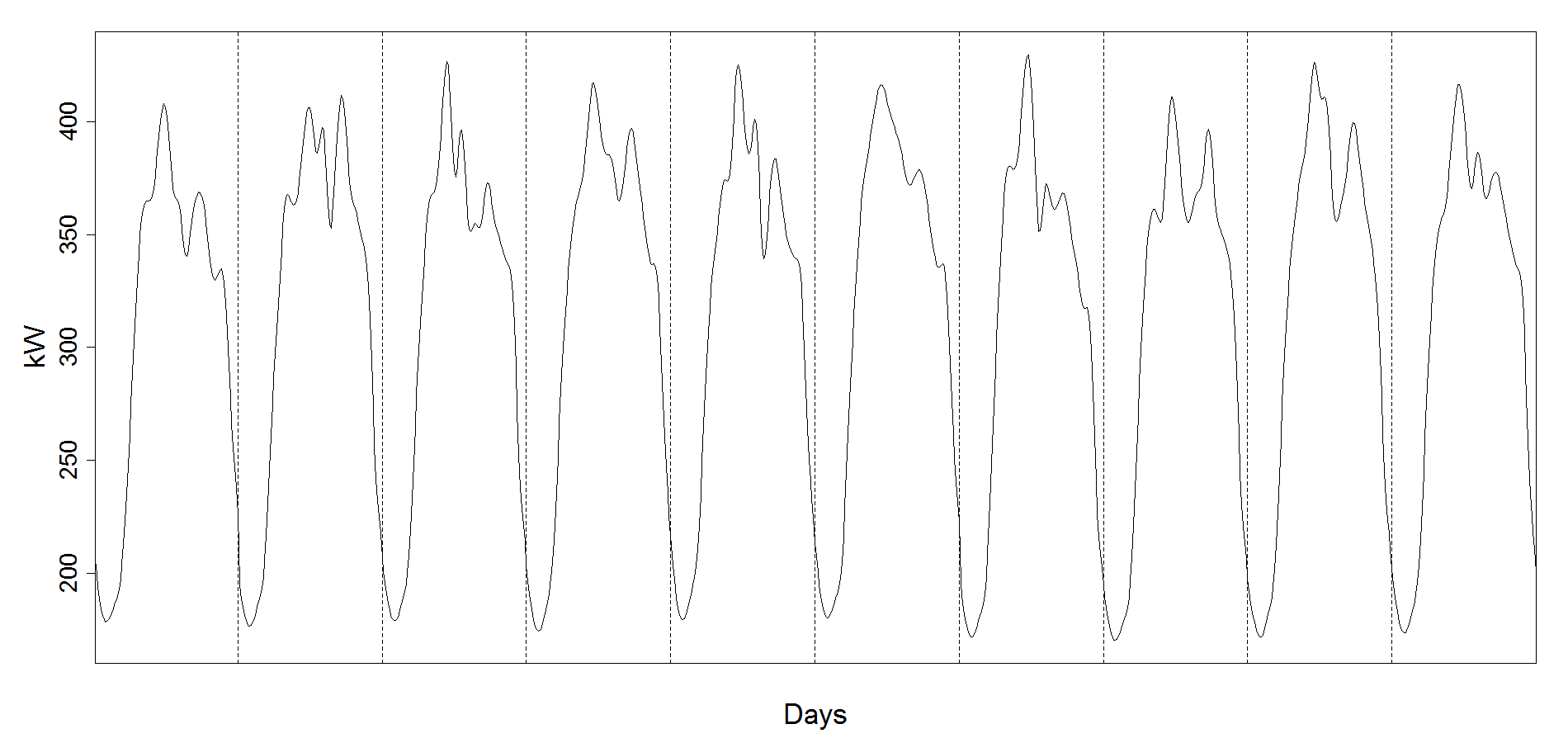
Figure 1: 10 consecutive daily load curves $X_{115}(t),\ldots,X_{124}(t)$ without weekends.

In order to apply the testing procedure we proceed as described in Section 5 and represent the discrete daily records as functional objects in rescaled time $t\in[0,1]$ using 25 $B$-Spline basis-functions, hereby smoothing the data. In the next step, in view of the obviously different stochastic pattern, we remove all curves which correspond to weekends. The remaining dataset consists of 261 curves $X_{1}(t),\ldots,X_{261}(t)$ corresponding to workdays (cf. Figure 2). Now, to gain stationarity, all curves are $\log$-transformed via

$$\tilde{X}_{i}(t)=\log(X_{i}(t)/X_{i}(0)).$$

For a discussion on this transformation we refer to Horváth & Rice (2015). In a third step, we discard the observations $\tilde{X}_{1}(t),\ldots,\tilde{X}_{100}$ (i.e. the data before May 21st) which show a somewhat too erratic behavior to be reasonable for our analysis.

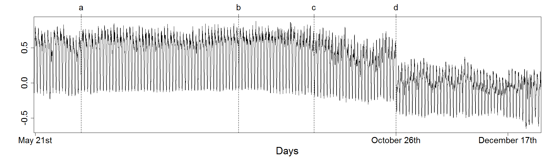
Figure 2: Consecutive daily $\log$-transformed load curves $\tilde{X}_{101}(t),\ldots,\tilde{X}_{261}(t)$ corresponding to workdays in the time period May 21st - December 31st in 2012.

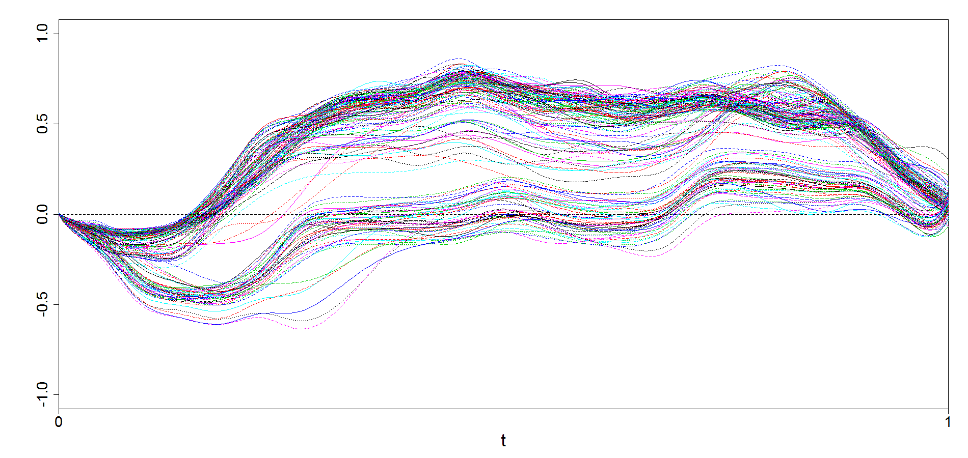
Figure 3: Daily $\log$-transformed load curves $\tilde{X}_{i}(t)$ for the low voltage electricity grid corresponding to workdays in the time period May 21st - December 31st in 2012. Lower curves correspond to the winter months. This is the »functional representation« of the time series from Figure 2.

The remaining observations $\tilde{X}_{101}(t),\ldots,\tilde{X}_{261}(t)$ exhibit an obvious large abrupt change in the mean at $\tilde{X}_{216}$, i.e. at line »d« in Figure 2, and a quite stationary behavior before and after the jump.

Data analysis:

Due to the large jump, we expect the procedure to reject the null hypothesis distinctly (the slight trend in segment »c - d« of Figure 2 should not affect the performance), which is confirmed in Table 5: the procedure rejects the null hypothesis for a wide range of parameters (where the $p$-values are based on approximation (5.4)). The tests are carried out using a plain kernel $K(x)=1_{[-1,1]}(x)$, different bandwidths $h=0,\ldots,4$ and various subspace dimensions $d=1,\ldots,6$. (Recall that we divide by $h$ in (4.1) and $h=0$ is thus formally prohibited. Here, we set $\hat{\zeta}(t,s)=\hat{\zeta}_{0}(t,s)$ for $h=0$.) Note that $\hat{T}_{n}$ is largest (or vice versa the $p$-values are smallest) for $h=0$, i.e. when the dependence structure is not taken into account. However, the results for $h>0$ should be more reliable since there seem to be indicators of dependencies in the data described in the following. We performed a basic analysis and checked for independence using the functional »Portmanteau Test of Independence« of Gabrys & Kokoszka (2007) which is also based on a dimension-reduction approach using (static) functional principal components. First, note that this procedure already requires mean zero data. Therefore, to minimize the influence of obvious large changes and of less obvious smaller trends we restrict our considerations to the rather homogeneous segment $\tilde{X}_{115}(t),\ldots,\tilde{X}_{190}(t)$ (i.e. segment »a - c« in Figure 2) and center this subsample by its sample mean. The test for this sample yields small $p$-values $<10^{-10}$ for a range of parameters $d$ (number of principal components) and $\tilde{H}$ (maximum lag). We obtain somewhat larger, but still small, $p$-values (cf. Table 6) if we restrict ourselves further to the segment $\tilde{X}_{115}(t),\ldots,\tilde{X}_{165}(t)$, (i.e. segment »a - b« in Figure 2.)

Table 5: Values of $\hat{T}_{n}$ for the load profile dataset. $p$-values are given in brackets.

$d$		$h=0$	$h=1$	$h=2$	$h=3$	$h=4$
1		$12.09\;(<0.0001)$	$7.08\;(<0.0001)$	$5.53\;(<0.0001)$	$4.70\;(0.0001)$	$4.17\;(0.0014)$
2		$12.17\;(<0.0001)$	$7.14\;(<0.0001)$	$5.58\;(<0.0001)$	$4.75\;(0.0007)$	$4.23\;(0.0057)$
3		$12.18\;(<0.0001)$	$7.14\;(<0.0001)$	$5.80\;(<0.0001)$	$4.75\;(0.0025)$	$4.23\;(0.0179)$
4		$12.34\;(<0.0001)$	$7.22\;(<0.0001)$	$5.91\;(<0.0001)$	$5.37\;(0.0005)$	$5.09\;(0.0018)$
5		$12.38\;(<0.0001)$	$7.43\;(<0.0001)$	$5.92\;(<0.0001)$	$5.43\;(0.0011)$	$5.20\;(0.0029)$
6		$12.62\;(<0.0001)$	$7.51\;(<0.0001)$	$5.96\;(0.0002)$	$5.48\;(0.0021)$	$5.29\;(0.0048)$

Table 6: $p$-values from the Portmanteau Test of Independence of Gabrys & Kokoszka (2007) applied to the segment $\tilde{X}_{115}(t),\ldots,\tilde{X}_{165}(t)$ of the load profile dataset. $d$ represents the number of principal components and $\tilde{H}$ denotes the maximum lag used for the test.

$\tilde{H}$		$d=1$	$d=2$	$d=3$	$d=4$
1		$0.0011$	$0.0228$	$0.0002$	$0.0023$
2		$<0.0001$	$0.0025$	$<0.0001$	$<0.0001$
3		$<0.0001$	$0.0021$	$<0.0001$	$<0.0001$

Remark 5.1.

Note that the curves in Figure 2 and Figure 3 which correspond to the winter months are below those corresponding to summer moths, due to the »functional rescaling« $X_{i}(t)/X_{i}(0)$ for $t\in[0,1]$: The electricity demand during morning and daytime in winter and summer months is comparable. However, in the winter the demand in the evening and especially at midnight, i.e. at $X_{i}(0)$, is much higher. Hence, the observed change is in accordance with the fact that electricity consumption in the winter is higher than in the summer and is most likely due to a switch in the »supply regime«.

Proofs

Proof of Theorem 3.4.

We outline the important steps, thereby following the proof of Torgovitski (2014, Theorem 4.1), which in turn is largely based on considerations of Berkes et al.​ (2009).

First, we replace the eigenfunctions with their estimates. Going through the proofs of Lemmas 6.4 and 6.5 of Torgovitski (2014) we see that (P1) and (A2) ensure that, as $n\rightarrow\infty$,

$$|T_{n}(X;\hat{v},\lambda)-T_{n}(Y;v,\lambda)|=o_{P}((\log\log n)^{-1/2})$$ (6.1)

and therefore, taking (L) into account

$$\lim_{n\rightarrow\infty}P\left(a(\log n)T_{n}(X;\hat{v},\lambda)-b_{d}(\log n)\leq x\right)=\exp(-2\exp(-x))$$ (6.2)

holds true. Next, we replace the population eigenvalues with their empirical versions. (A1) implies that $\lim_{n\rightarrow\infty}P(\hat{\lambda}_{d}>c)=1$, for some $c>0$, and that $\max_{i=1,\ldots,d}|\hat{\lambda}^{-1/2}_{i}-\lambda^{-1/2}_{i}|=o_{P}((\log\log n)^{-1})$ hold true. Following the arguments of Torgovitski (2014, Lemma 6.7) we see that (6.2) and (A1) imply that

$$|T_{n}(X;\hat{v},\hat{\lambda})-T_{n}(X;\hat{v},\lambda)|=o_{P}((\log\log n)^{-1/2}).$$

The assertion follows immediately by using (6.1) and (L). ∎

Proof of Theorem 3.7.

Let $m={\lfloor n\theta\rfloor}$. It is clear that

$$\sum_{i=1}^{k}\Big{(}X_{i}(t)-\bar{X}_{n}(t)\Big{)}=\sum_{i=1}^{k}\Big{(}Y_{i}(t)-\bar{Y}_{n}(t)\Big{)}-\frac{k}{n}(n-m)\Delta(t)$$ (6.3)

holds true for $1\leq k\leq m$. Hence, using standard arguments we obtain that

$$\hat{T}_{n} \geq c_{1}w(m/n)\bigg{\{}\Big{|}\int\!n^{-1/2}\sum_{i=1}^{m}(X_{i}(t)-\bar{X}_{n}(t))\hat{v}_{r}(t)dt\Big{|}\bigg{\}}/\hat{\lambda}^{1/2}_{r}$$

$$\geq c_{2}w(\theta)\bigg{\{}\bigg{|}\big{|}\int\!n^{-1}\sum_{i=1}^{m}(Y_{i}(t)-\bar{Y}_{n}(t))\hat{v}_{r}(t)dt\big{|}$$

$$-\bigg{[}|\int\!\Delta(t)\hat{v}_{r}(t)dt|-\xi\bigg{]}m(n-m)/\big{(}n^{3/2}n^{1/2}\big{)}$$

$$\quad+\xi m(n-m)/n^{2}\bigg{|}\bigg{\}}\times\bigg{[}(\log\log n)^{1/2}n^{1/2}/\big{(}(\log\log n)^{1/2}\hat{\lambda}_{r}^{1/2}\big{)}\bigg{]}$$

$$=:c_{2}w(\theta)\big{|}A_{1}+A_{2}+A_{3}\big{|}(\log\log n)^{1/2}\big{(}(\hat{\lambda}_{r}\log\log n)/n\big{)}^{-1/2}$$

for some $c_{1},c_{2}>0$. We get $A_{1}=o_{P}(1)$ in view of (P2), $\|\hat{v}_{r}\|=1$ and due to the Cauchy-Schwarz inequality. Further, $A_{2}=o_{P}(1)$ holds true on account of (B2). The third term $A_{3}$ converges towards a nonzero (positive) constant, again due to $\xi>0$ in (B2). The assertion follows now in view of (B1). ∎

Proof of Theorem 3.8.

We carry over and adapt the arguments of Csörgő & Horváth (1997, Theorem 2.8.1) to our functional setting. (E1) particularly implies that $P(\hat{\lambda}_{d}>0)$ is tending to 1 under $H_{A}$. Thus, for convenience we tacitly restrict the consideration to the set where $\hat{\lambda}_{d}>0$ holds true.

Following the notation in (3.5) we write $\hat{\mathbf{X}}_{i}$, $\hat{\mathbf{Y}}_{i}$ and $\hat{\boldsymbol{\mu}}_{i}$ for vectors where the $r$-th components are the scores $\hat{\mathbf{X}}_{i,r}=\int\!X_{i}(t)\hat{v}_{r}(t)dt$, $\hat{\mathbf{Y}}_{i,r}=\int\!Y_{i}(t)\hat{v}_{r}(t)dt$ and $\hat{\boldsymbol{\mu}}_{i,r}=\int\!\mu_{i}(t)\hat{v}_{r}(t)dt$. Furthermore, we set $\hat{\boldsymbol{\Delta}}=\hat{\boldsymbol{\mu}}_{n}-\hat{\boldsymbol{\mu}}_{1}$. Using the Cauchy-Schwarz inequality and (P1) we have

$$\max_{1\leq k<n}w(k/n)\bigg{|}\int\!n^{-1/2}\sum_{i=1}^{k}(Y_{i}(t)-\bar{Y}_{n}(t))\hat{v}_{r}(t)dt\bigg{|}$$

$$\leq\|\hat{v}_{r}\|\max_{1\leq k<n}w(k/n)\Big{\|}n^{-1/2}\sum_{i=1}^{k}(Y_{i}-\bar{Y}_{n})\Big{\|}={\mathcal{O}}_{P}(g(n))$$

for all $1\leq r\leq d$. The rate $g(n)$ follows by using the same arguments as in (Torgovitski, 2014, Lemma 6.2), i.e. relying on stationarity of the innovations and using the symmetry of the test statistic. Hence, as a direct consequence we get

$$\max_{1\leq k<n}w(k/n)|n^{-1/2}\sum_{i=1}^{k}(\hat{\mathbf{Y}}_{i}-\bar{\hat{\mathbf{Y}}}_{n})|_{\hat{{\mathbf{\Sigma}}}}=\hat{\lambda}_{d}^{-1/2}{\mathcal{O}}_{P}(g(n)).$$

for the projected counterpart. Set $m={\lfloor n\theta\rfloor}$ as before and observe that

$$\max_{1\leq k<m-\lfloor n\alpha\rfloor}\left(\frac{k}{n-k}\right)\begin{cases}=m/(n-m),&\alpha=0,\\ \leq(m-n\alpha)/(n-m),&0<\alpha<\theta.\end{cases}$$ (6.4)

Now, on one hand, by taking (6.3) and $w(k/n)k/n=(k/(n-k))^{1/2}$ into account and by considering the square root version of (6.4) we get

$$\max_{1\leq k<m-\lfloor n\alpha\rfloor}w(k/n)|\sum_{i=1}^{k}(\hat{\mathbf{X}}_{i}-\bar{\hat{\mathbf{X}}}_{n})|_{\hat{{\mathbf{\Sigma}}}}$$

$$\leq\max_{1\leq k<m}w(k/n)|\sum_{i=1}^{k}(\hat{\mathbf{Y}}_{i}-\bar{\hat{\mathbf{Y}}}_{n})|_{\hat{{\mathbf{\Sigma}}}}+|\hat{\boldsymbol{\Delta}}|_{\hat{{\mathbf{\Sigma}}}}\max_{1\leq k<m-n\alpha}w(k/n)\frac{k}{n}(n-m)$$

$$={\mathcal{O}}_{P}\left(n^{1/2}g(n)/\hat{\lambda}_{d}^{1/2}\right)+(n-m)^{1/2}(m-n\alpha)^{1/2}|\hat{\boldsymbol{\Delta}}|_{\hat{{\mathbf{\Sigma}}}}$$

for $\alpha\in[0,\theta)$. Whereas, on the other hand, we arrive at

$$\max_{1\leq k<m}w(k/n)|\sum_{i=1}^{k}(\hat{\mathbf{X}}_{i}-\bar{\hat{\mathbf{X}}}_{n})|_{\hat{{\mathbf{\Sigma}}}}$$

$$\geq\bigg{|}\max_{1\leq k<m}w(k/n)|\sum_{i=1}^{k}(\hat{\mathbf{Y}}_{i}-\bar{\hat{\mathbf{Y}}}_{n})|_{\hat{{\mathbf{\Sigma}}}}-|\hat{\boldsymbol{\Delta}}|_{\hat{{\mathbf{\Sigma}}}}\max_{1\leq k<m}w(k/n)\frac{k}{n}(n-m)\bigg{|}$$

$$=\bigg{|}A_{1}-|\hat{\boldsymbol{\Delta}}|_{\hat{{\mathbf{\Sigma}}}}(n/w(m/n))\bigg{|},$$

where $A_{1}={\mathcal{O}}_{P}\left(n^{1/2}g(n)/\hat{\lambda}_{d}^{1/2}\right)$, as before. (E1) and (B2) ensure that

$$\frac{n^{1/2}g(n)/\hat{\lambda}_{d}^{1/2}}{|\hat{\boldsymbol{\Delta}}|_{\hat{{\mathbf{\Sigma}}}}(n/w(m/n))}\leq\frac{c}{\big{|}\int\!\Delta(t)\hat{v}_{r}(t)dt\big{|}}\frac{g(n)}{n^{1/2}}\Bigg{[}\frac{\hat{\lambda}_{1}}{\hat{\lambda}_{d}}\Bigg{]}^{1/2}=o_{P}(1)$$

for some $c>0$ since $|\hat{\boldsymbol{\Delta}}|^{-1}_{\hat{{\mathbf{\Sigma}}}}\geq\hat{\lambda}_{1}^{-1/2}|\int\!\Delta(t)\hat{v}_{j}(t)dt|$ for $j=1,\ldots,d$. Altogether, we obtain

$$\frac{\max_{1\leq k<m-\lfloor n\alpha\rfloor}w(k/n)|\sum_{i=1}^{k}(\hat{\mathbf{X}}_{i}-\bar{\hat{\mathbf{X}}}_{n})|_{\hat{{\mathbf{\Sigma}}}}}{|\hat{\boldsymbol{\Delta}}|_{\hat{{\mathbf{\Sigma}}}}(n/w(m/n))}\begin{cases}=1+o_{P}(1),&\alpha=0\\ \leq(1-\alpha/\theta)^{1/2}+o_{P}(1),&0<\alpha<\theta\end{cases}$$

which completes this proof. ∎

Proof of Theorem 3.10.

Property (3.2) is stated in Theorem 1 of Horváth et al.​ (2013) and (P2) follows from ergodicity and stationarity. However, note that (P2) is also immediately implied by Berkes et al.​ (2013, Theorem 3.3). We proceed with the verification of (L). Going carefully through the proof of Csörgő & Horváth (1997, Theorem 4.1.3) and taking Schmitz (2011, Theorem 2.1.4) into account - replacing all considerations for univariate time series with multivariate analogues - we see that it suffices to show the conditions (C1), (C2) and (C3) below (cf. also Kamgaing & Kirch (2016, Theorem 1.2.1)). Hereby, it is crucial that $L^{\kappa}$-$m$-approximable time series fulfill (M) by definition. For one thing, we need an approximation of the projected innovations $\{\mathbf{Y}_{i}\}$ (see (3.5)) by centered multivariate Brownian motions $\{\mathbf{W}_{1}(n)\}$, $\{\mathbf{W}_{2}(n)\}$ with covariance matrix ${\mathbf{\Sigma}}$ (cf. 3.2). More precise, we need that

$$\Big{|}\sum_{i=1}^{n}\mathbf{Y}_{i}-\mathbf{W}_{1}(n)\Big{|} ={\mathcal{O}}(n^{1/2-\eta})\qquad\text{a.s.},$$ (C1)

$$\Big{|}\sum_{i=1}^{n}\mathbf{Y}_{-i}-\mathbf{W}_{2}(n)\Big{|} ={\mathcal{O}}(n^{1/2-\eta})\qquad\text{a.s.}$$ (C2)

for some $\eta>0$. (We do not impose any restriction on the dependence structure between $\{\mathbf{W}_{1}(n)\}$ and $\{\mathbf{W}_{2}(n)\}$). For another thing, we need the asymptotic independence as well as the exact asymptotic distributions of

$$A_{n}^{*} :=a(\log n)A_{n}-b_{d}(\log n),$$

$$B_{n}^{*} :=a(\log n)B_{n}-b_{d}(\log n)$$

with

$$A_{n} =\max_{1\leq k\leq n/\log n}k^{-1/2}\bigg{|}\sum_{i=1}^{k}\mathbf{Y}_{i}\bigg{|},$$

$$B_{n} =\max_{n-n/\log n\leq k<n}(n-k)^{-1/2}\bigg{|}\sum_{i=k+1}^{n}\mathbf{Y}_{i}\bigg{|},$$

i.e. that

$$\begin{split}\lim_{n\rightarrow\infty}P(A^{*}_{n}\leq s,B^{*}_{n}\leq t)&=\lim_{n\rightarrow\infty}P(A^{*}_{n}\leq s)P(B^{*}_{n}\leq t)\\ &=\exp(-\exp(-s))\exp(-\exp(-t))\end{split}$$ (C3)

holds true for all $s,t\in\mathbb{R}$.

These conditions (C1), (C2) and (C3) are analogous to conditions A.3 (i)-(iii) of Kamgaing & Kirch (2016, Theorem 1.2.1). Condition (C1) replaces Assumption A.3 (i), (C2) corresponds to Assumption A.3 (ii) of Kamgaing & Kirch (2016) and condition (C3) corresponds to Assumption A.3 (iii) (up to normalizing sequences $a(\log n)$ and $b_{d}(\log n)$, cf. Csörgő & Horváth (1997, Theorem 4.1.3)). Notice that the additional Assumption A.1 of Kamgaing & Kirch (2016) is trivially fulfilled in our setting, due to the shape of our test statistic.

We begin by discussing and verifying $\eqref{C1}$. It is easy to see, that the projected time series $\{\mathbf{Y}_{i}\}_{i\in\mathbb{Z}}$ remains $L^{\kappa}$-$m$-approximable (now in $\mathbb{R}^{d}$) with same $\kappa>2$ and same rate $\delta(m)$. In particular $E\|Y_{0}\|^{\kappa}<\infty$, $\kappa>2$, holds true and ${\mathbf{\Sigma}}$ is obviously positive definite due to $\lambda_{d}>0$ (cf. also 3.2). Hence, $\eqref{C1}$ follows immediately from Theorem A.1 of Aue et al.​ (2014, cf. Theorem S2.1 in the supplement) taking Csörgő & Horváth (1997, disp. (A.1.16)) into account. Furthermore, a careful examination of the proof of Aue et al.​ (2014, Theorem A.1) shows that their arguments do not rely on causality and their strong approximation in Theorem A.1 could be restated for general (noncausal) $L^{\kappa}$-$m$-approximable multivariate time series using 2.1 with $H=\mathbb{R}^{d}$ and $\delta(m)=m^{-\gamma}$ for some $\gamma>2$. Note that in the proof of Theorem A.1 of Aue et al.​ (2014), coupling expressions like, e.g.,

$$E[\mathbf{Y}_{0,r}\mathbf{Y}_{j,r}]=E\big{[}\mathbf{Y}_{0,r}(\mathbf{Y}_{j,r}-\mathbf{Y}_{j,r}^{(j)})\big{]},$$

are only valid under causality, since $E[\mathbf{Y}_{0,r}\mathbf{Y}_{j,r}^{(j)}]=0$ is necessary. However, relation $\smash{E[\mathbf{Y}^{(j)}_{0,r}\mathbf{Y}_{j,r}^{(j)}]=0}$ is valid under noncausality and it is known that the above expression can be easily replaced by

$$E[\mathbf{Y}_{0,r}\mathbf{Y}_{j,r}]=E\big{[}\mathbf{Y}_{j,r}(\mathbf{Y}_{0,r}-\mathbf{Y}_{0,r}^{(j)})\big{]}+E\big{[}\mathbf{Y}^{(j)}_{0,r}(\mathbf{Y}_{j,r}-\mathbf{Y}_{j,r}^{(j)})\big{]}.$$ (6.5)

Now, observe that after time inversion $\{\mathbf{Y}_{-i}\}_{i\in\mathbb{Z}}$ remains $L^{\kappa}$-$m$-approximable (in the sense of 2.1) with the same $\kappa$, the same rate $\delta(m)$ and with the same long run covariance matrix ${\mathbf{\Sigma}}$. Hence, according to previous considerations, (C2) holds true, as well.

Finally, we verify (C3). In the setting of linear processes, Csörgő & Horváth (1997, Theorem 4.1.3) have shown asymptotic independence of $A_{n}$ and $B_{n}$ by replacing the $\mathbf{Y}_{i}$’s in $B_{n}$ by truncated approximations (cf. Csörgő & Horváth (1997, p.308)). We adapt this approach in a straightforward manner by considering $m$-dependent copies $\mathbf{Y}_{i}^{(m)}$ (cf. (2.3)) and defining

$$B_{n}^{\prime}:=\max_{n-n/\log n\leq k<n}(n-k)^{-1/2}|\sum_{i=k+1}^{n}\mathbf{Y}_{i}^{(m_{n})}|,$$

where $m_{n}:=n-3n/\log n$. The representation of $\mathbf{Y}_{i}$’s as a shift of i.i.d. random variables and the construction of the $\mathbf{Y}^{(m_{n})}_{i}$’s ensures that $Z_{k,r}:=\mathbf{Y}_{k,r}-\mathbf{Y}_{k,r}^{(m_{n})}$ are equally distributed for all $k$. Hence, it holds that

$$E|Z_{k,r}|^{2}=E|Z_{0,r}|^{2}={\mathcal{O}}(m_{n}^{-2\gamma})$$

for all $k\in\mathbb{Z}$ and $r=1,\ldots,d$. Furthermore,

$$|B_{n}-B_{n}^{\prime}| \leq\max_{n-n/\log n\leq k<n}(n-k)^{-1/2}\Big{|}\sum_{i=k+1}^{n}\left(\mathbf{Y}_{i}-\mathbf{Y}_{i}^{(m_{n})}\right)\Big{|}$$

$$\leq d\sum_{r=1}^{d}\left(\max_{n-n/\log n\leq k<n}(n-k)^{-1/2}\big{|}\sum_{i=k+1}^{n}Z_{i,r}\big{|}\right).$$

An application of the Hájeck-Rényi type inequality of Kounias & Weng (1969, Theorem 2) yields that

$$P\bigg{(}\max_{n-n/\log n\leq k<n}(n-k)^{-1/2}\big{|}\sum_{i=k+1}^{n}Z_{i,r}\big{|}>(\log n)^{-1/2}\bigg{)}$$

$$\leq\bigg{(}(\log n)^{1/2}\sum_{k=n-n/\log n}^{n-1}(n-k)^{-1/2}\big{(}E|Z_{k,r}|^{2}\big{)}^{1/2}\bigg{)}^{2}$$

$$=(\log n)E|Z_{0,r}|^{2}\bigg{(}\sum_{k=1}^{n/\log n}k^{-1/2}\bigg{)}^{2}={\mathcal{O}}\left((\log n)m_{n}^{-2\nu}\frac{n}{\log n}\right)={\mathcal{O}}(n^{1-2\nu}),$$

which implies

$$B_{n}=B_{n}^{\prime}+o_{P}(a(\log n)^{-1}).$$

Now, observe that $B_{n}^{\prime}$ and $A_{n}$ are independent because the sets $\{\mathbf{Y}_{i},i\leq n/\log n\}$ and $\smash{\{\mathbf{Y}_{i}^{(m_{n})},i\geq n-n/\log n,\;m_{n}=n-3n/\log n\}}$ are obviously independent for sufficiently large $n$. Finally, (C3) follows from Horváth (1993, Lemma 2.2) taking Davidson (1994, Lemma 29.5) into account. ∎

Proof of 3.11.

The well known results of Móricz (1976) show that moment inequalities for partial sums yield analogous moment inequalities for maxima of partial sums. Furthermore, in Tómács and Líbor (2006) it is shown that inequalities for maxima of partial sums yield inequalities for weighted maxima of partial sums and vice versa. Carefully inspecting the proofs of Móricz (1976, Theorem 1) and of Tómács and Líbor (2006, Theorem 2.1) we observe that the same results can be restated in our functional setting with $\kappa>2$, as well. Therefore, Móricz (1976, Theorem 1) together with assumption (3.15) and Markov’s inequality yield

$$x^{\kappa}P\left(\max_{1\leq k\leq n}\big{\|}\sum_{i=1}^{k}Y_{i}\big{\|}\geq x\right)\leq E\bigg{[}\max_{1\leq k\leq n}\big{\|}\sum_{i=1}^{k}Y_{i}\big{\|}^{\kappa}\bigg{]}\leq c_{1}n^{\kappa/2}$$ (6.6)

for all $x>0$, $n\in\mathbb{N}$ and some $c_{1}>0$. Next, we use $n^{\kappa/2}={\mathcal{O}}(\sum_{k=1}^{n}k^{\kappa/2-1})$ and apply Tómács and Líbor (2006, Theorem 2.1) to obtain,

$$x^{\kappa}P\left(\max_{1\leq k\leq n}k^{-1/2}\big{\|}\sum_{i=1}^{k}Y_{i}\big{\|}\geq x\right)\leq c_{2}\sum_{k=1}^{n}k^{-1}\leq c_{3}\log n,$$

for all $x>0$, $n\in\mathbb{N}$ and some $c_{2}$, $c_{3}>0$. The conclusion follows on setting $x=c_{4}(\log n)^{1/\kappa}$ with a suitable constant $c_{4}>0$. ∎

Remark 6.1.

In the previous proof we applied Móricz (1976, Theorem 1) with $g(F_{b,n})=n^{\alpha}$, $b=0$ and $\alpha=\kappa/2>1$. In case of $\kappa=2$ (i.e. $\alpha=1$) an additional logarithmic term would appear on the right-hand side of (6.6) (cf. Móricz (1976, Theorem 3)).

We proceed with the proof of 3.12. Berkes et al.​ (2011, Proposition 4) have shown the corresponding result in the univariate setting and their techniques, slightly modified, are directly applicable to the functional setting, as shown below. Here, we demonstrate that Proposition 4 of Berkes et al.​ (2011) is extensible to noncausal centered $L^{\kappa}$-$m$-approximable functional time series $\{Y_{i}\}_{i\in\mathbb{Z}}$. We want to emphasize that another, more sophisticated extension - yet for causal centered $L^{\kappa}$-$m$-approximable time series -, has been developed by Berkes et al.​ (2013, cf. Theorems 3.1, 3.3 and Remark 3.2).

Proof of 3.12.

We want to point out that - up to the functional setting - the proof presented here is for most parts identical with Berkes et al.​ (2011, Proposition 4) and that we stay very close to their exposition. To avoid misunderstandings and for the convenience of the reader, we restate their proof in the functional setting, emphasizing the necessary modifications. In adaption to our situation, the major difficulty stems from the relations (37) - (39) of Berkes et al.​ (2011) which are not clear in the functional setting for arbitrary $\kappa>2$ and therefore are substituted by (6.13) below. This is done using a result of Berkes et al.​ (2013) which is, however, restricted to $\kappa\in(2,3)$.

Let $S_{n}=\sum_{i=1}^{n}Y_{i}$ denote the partial sums, let $\psi_{2}>0$, $\psi_{\kappa}>0$ be arbitrary constants and let

$$D_{\kappa}:=\sum_{m=0}^{\infty}(E\|X_{0}-X_{0}^{(m)}\|^{\kappa})^{1/\kappa}<\infty,$$

where the finiteness holds true in view of $\sum_{m=1}^{\infty}\delta(m)<\infty$. The cases $\kappa=2$ and $2<\kappa<3$ are treated separately, where the former one can be seen as follows: Via the decomposition

$$Y_{0}(t)Y_{j}(s)=\Big{(}Y_{0}(t)-Y_{0}^{(j)}(t)\Big{)}Y_{j}(s)+Y^{(j)}_{0}(t)\Big{(}Y_{j}(s)-Y_{j}^{(j)}(s)\Big{)}+Y_{0}^{(j)}(t)Y_{j}^{(j)}(s),$$

using stationarity and $D_{2}<\infty$ we obtain

$$E\|S_{n}\|^{2}=\sum_{k=1}^{n}E\int\!Y_{k}(t)Y_{k}(t)dt+2\!\!\sum_{1\leq k<l\leq n}E\int\!Y_{k}(t)Y_{l}(t)dt\leq nC_{2}$$ (6.7)

for some $C_{2}>D_{2}/\psi_{2}$ and all $n\in\mathbb{N}$, which finishes the proof for $\kappa=2$. For more details cf. Berkes et al.​ (2011). For the latter case, i.e. $2<\kappa<3$, the idea is to show, that for any $n_{0}\in\mathbb{N}$ there is some $C_{\kappa}(n_{0})$ such that:

$$E\|S_{n}\|^{\kappa}\leq C_{\kappa}n^{\kappa/2}\quad\forall n\leq n_{0}\qquad\Rightarrow\qquad E\|S_{n}\|^{\kappa}\leq C_{\kappa}n^{\kappa/2}\quad\forall n\leq 2n_{0}.$$ (6.8)

Hence, by induction, it is possible to conclude that $C_{\kappa}$ does not depend on $n_{0}$ which then completes the proof.

Now, (6.8) can be verified by selecting an arbitrary $n_{0}\in\mathbb{N}$ and choosing $C_{\kappa}(n_{0})$ large enough, such that on the one hand

$$E\|S_{n}\|^{\kappa}\leq C_{\kappa}(n_{0})n^{\kappa/2}$$ (6.9)

for all $n\leq n_{0}$ and on the other hand $C^{1/\kappa}_{\kappa}(n_{0})>D_{\kappa}/\psi_{\kappa}$. Using Jensen’s inequality we have

$$E\|Y_{k}-Y_{k}^{(n-k)}\|\leq(E\|Y_{k}-Y_{k}^{(n-k)}\|^{\kappa})^{1/\kappa},$$

which, via basic inequalities for norms, yields that

$$E\|S_{2n}\|^{\kappa}\leq\left(2D_{\kappa}+\left(E\bigg{[}\|Z_{n}+W_{n}\|^{\kappa}\bigg{]}\right)^{1/\kappa}\right)^{\kappa}$$ (6.10)

where

$$Z_{n}=\sum_{k=1}^{n}Y_{k}^{(n-k)},\qquad W_{n}=\sum_{k=1}^{n}Y_{n+k}^{(k-1)}$$

(cf. Berkes et al.​ (2011, disp. (36))). Next, observe that

$$E\|Z_{n}\|^{p}\leq\left(\bigg{(}E\|S_{n}\|^{p}\bigg{)}^{1/p}+D_{p}\right)^{p}$$

for $p=2$ or $p=\kappa$, respectively, and that the same holds true if we replace $W_{n}$ by $Z_{n}$. Hence, in view of (6.9), we arrive at

$$\begin{split}E\|Z_{n}\|^{\kappa}&\leq n^{\kappa/2}C_{\kappa}(1+\psi_{\kappa})^{\kappa},\\ E\|W_{n}\|^{\kappa}&\leq n^{\kappa/2}C_{\kappa}(1+\psi_{\kappa})^{\kappa},\\ \end{split}$$ (6.11)

for $n\leq n_{0}$. Furthermore, due to (6.7) it holds also that

$$\begin{split}E\|Z_{n}\|^{2}&\leq nC_{2}(1+\psi_{2})^{2},\\ E\|W_{n}\|^{2}&\leq nC_{2}(1+\psi_{2})^{2},\end{split}$$ (6.12)

for all $n\in\mathbb{N}$ (cf. Berkes et al.​ (2011)). Recall that $C^{1/2}_{2}>D_{2}/\psi_{2}$ and that no restriction on $n$ is needed here due to (6.7). Observe that $Z_{n}$ and $W_{n}$ are mean zero and independent. Therefore, by Berkes et al.​ (2013, Lemma 3.1) we have for $2<\kappa<3$ that

$$\begin{split}E\|Z_{n}+W_{n}\|^{\kappa}&\leq E\|Z_{n}\|^{\kappa}+E\|W_{n}\|^{\kappa}\\ &\quad+E\|Z_{n}\|^{2}(E\|W_{n}\|^{2})^{\kappa/2-1}\\ &\quad+E\|W_{n}\|^{2}(E\|Z_{n}\|^{2})^{\kappa/2-1}.\end{split}$$ (6.13)

Now, combining (6.11), (6.12) and (6.13) yields

$$E\|Z_{n}+W_{n}\|^{\kappa}\leq 2(1+\psi_{\kappa})^{\kappa}C_{\kappa}n^{\kappa/2}+2\left((1+\psi_{2})^{2}C_{2}n\right)^{\kappa/2}$$ (6.14)

for all $n\leq n_{0}$, which is a simple but significant modification of Berkes et al.​ (2011, disp. (37)). Consequently, from (6.10) and (6.14) we obtain

$$E\|S_{2n}\|^{\kappa} \leq\left\{2D_{\kappa}+\left(E\|Z_{n}+W_{n}\|^{\kappa}\right)^{1/\kappa}\right\}^{\kappa}$$

$$\leq\left\{2D_{\kappa}+\left(2(1+\psi_{\kappa})^{\kappa}C_{\kappa}n^{\kappa/2}+2\left((1+\psi_{2})^{2}C_{2}n\right)^{\kappa/2}\right)^{1/\kappa}\right\}^{\kappa}$$

$$\leq C_{\kappa}(n\Psi)^{\kappa/2}$$

where

$$\Psi(\psi_{\kappa},\psi_{2},C_{\kappa},C_{2}):=2\psi_{\kappa}+\left[2(1+\psi_{\kappa})^{\kappa}+2(1+\psi_{2})^{\kappa}C_{2}^{\kappa/2}C_{\kappa}^{-1}\right]^{1/\kappa}\downarrow 2^{1/\kappa}<2$$

as $(\psi_{2},\psi_{\kappa},C_{\kappa}^{-1})\rightarrow 0$ (cf. Berkes et al.​ (2011, disp. (38))). Copying the final arguments of Berkes et al.​ (2011, Proof of Proposition 4) completes the proof. ∎

Next, we take a closer look at the estimation of the eigenstructure of ${\cal C}$.

Proof of Theorem 4.1.

Due to the symmetry of $K(x)$ the estimator $\hat{\zeta}$ can be rewritten as

$$\hat{\zeta}=\hat{\zeta}_{0}(t,s)+\sum_{i=1}^{n}K(i/h_{n})\hat{\zeta}_{i}(t,s)+\sum_{i=1}^{n}K(i/h_{n})\hat{\zeta}_{i}(s,t).$$ (6.15)

Note that in view of Hörmann & Kokoszka (2010, Theorem 3.1) the covariance estimation is of order

$$\iint(\hat{\zeta}_{0}(t,s)-E[Y_{0}(t)Y_{0}(s)])^{2}dtds={\mathcal{O}}_{P}(n^{-1}).$$ (6.16)

(Their arguments carry over to our case of noncausality in a straightforward manner using modifications similar to (6.5).) It remains to investigate the long run part of the estimate, where due to symmetry it suffices to consider the second term of (6.15). We define a centered version of the second expression of (6.15)

$$\hat{c}_{1,n}(t,s)=\sum_{i=1}^{n}K(i/h_{n})\hat{\gamma}_{i}(t,s)$$

with $\hat{\gamma}_{i}(t,s)=n^{-1}\sum_{j=1}^{n-i}Y_{j}(t)Y_{j+i}(s)$ and take into account that the difference between the original expression and its centered counterpart is of order

$$\iint\left(\sum_{i=1}^{n}K(i/h_{n})\hat{\zeta}_{i}(t,s)-\hat{c}_{1,n}(t,s)\right)^{2}dtds={\mathcal{O}}_{P}(h_{n}^{2}/n)$$ (6.17)

(cf. Horváth et al.​ (2013, proof of Theorem 2), as before, with straightforward modifications in view of noncausality). The centered version can be decomposed as follows:

$$\hat{c}_{1,n}-c_{1}=\left[\hat{c}_{1,n}-\hat{c}^{(m_{n})}_{1,n}\right]+\left[\hat{c}^{(m_{n})}_{1,n}-E\hat{c}^{(m_{n})}_{1,n}\right]+\left[E\hat{c}^{(m_{n})}_{1,n}-c^{(m_{n})}_{1}\right]+\left[c^{(m_{n})}_{1}-c_{1}\right],$$

where

$$c_{1}(t,s) =\sum_{i=1}^{\infty}E[Y_{0}(t)Y_{i}(s)],$$

$$c^{(m_{n})}_{1}(t,s) =\sum_{i=1}^{m_{n}}E[Y^{(m_{n})}_{0}(t)Y^{(m_{n})}_{i}(s)],$$

$$\hat{c}^{(m_{n})}_{1,n}(t,s) =\sum_{i=1}^{n}K(i/h_{n})\hat{\gamma}^{(m_{n})}_{i}(t,s),$$

$$\hat{\gamma}^{(m_{n})}_{i}(t,s) =n^{-1}\sum_{j=1}^{n-i}Y^{(m_{n})}_{j}(t)Y^{(m_{n})}_{j+i}(s)$$

and $(m_{n})$ indicates the $m_{n}$-dependent versions. The sequence $m_{n}$ needs to fulfill $m_{n}=o(h_{n})$ and $m_{n}\rightarrow\infty$, as $n\rightarrow\infty$. The main extension of the proof of Horváth et al.​ (2013) is the introduction of the additional term $E[\hat{c}^{(m_{n})}_{1,n}(t,s)]$ and that we allow for an increase in the dependency of $\hat{c}^{(m_{n})}_{1,n}(t,s)$ with increasing sample size $n\rightarrow\infty$. We proceed by observing that

$$\begin{split}&\bigg{|}{\rm Var}\bigg{(}\sum_{i=1}^{n}K(i/h_{n})\hat{\gamma}^{(m_{n})}_{i}(t,s)\bigg{)}\bigg{|}\\ &=\bigg{|}\sum_{i,j=1}^{n}{\rm Cov}\bigg{(}K(i/h_{n})\hat{\gamma}^{(m_{n})}_{i}(t,s),K(j/h_{n})\hat{\gamma}^{(m_{n})}_{j}(t,s)\bigg{)}\bigg{|}\\ &\leq c_{1}\sum_{i,j=1}^{n}\left|{\rm Cov}\left(\hat{\gamma}^{(m_{n})}_{i}(t,s),\hat{\gamma}^{(m_{n})}_{j}(t,s)\right)\right|\\ &\leq n^{-2}c_{1}\sum_{i,j=1}^{n}\sum_{k,r=1}^{n}\left|{\rm Cov}\left(Y^{(m_{n})}_{k}(t)Y^{(m_{n})}_{k+i}(s),Y^{(m_{n})}_{r}(t)Y^{(m_{n})}_{r+j}(s)\right)\right|\end{split}$$ (6.18)

for some $c_{1}>0$. Hence, (6.18), stationarity and $m_{n}$-dependence yield, by counting the independent terms and taking into account that $K(x)\equiv 0$ for $x>c$ for some $c>0$,

$$n^{2}\iint\bigg{|}{\rm Var}\left[\sum_{i=1}^{n}K(i/h_{n})\hat{\gamma}^{(m_{n})}_{i}(t,s)\right]\bigg{|}dtds={\mathcal{O}}(1)\sum_{i,j=1}^{\lfloor ch_{n}\rfloor}\sum_{k,r=1}^{n}\delta_{k,r}^{i,j},$$

where

$$\delta_{k,r}^{i,j}:=\begin{cases}0,&r-(k+i)\geq m_{n},r\geq k,\\ 0,&k-(r+j)\geq m_{n},r\leq k,\\ 1,&r-(k+i)\leq m_{n},r\geq k,\\ 1,&k-(r+j)\leq m_{n},r\leq k,\end{cases}\quad=\leavevmode\nobreak\ \begin{cases}1,&0\leq r-k\leq m_{n}+i,\\ 1,&0\leq k-r\leq m_{n}+j,\\ 0,&\text{else}.\end{cases}$$

Due to stationarity, the values $\delta_{k,r}^{i,j}$ depend only on $i$, $j$ and on the difference of $k-r$. Hence, we have

$$\sum_{i,j=1}^{\lfloor ch_{n}\rfloor}\sum_{k,r=1}^{n}\delta_{k,r}^{i,j} =\sum_{i,j=1}^{\lfloor ch_{n}\rfloor}\sum_{z=1}^{n}\left\{\sum_{q=0}^{n}\delta_{z,z+q}^{i,j}+\sum_{q=0}^{n}\delta_{z+q,z}^{i,j}\right\}$$

$$=\sum_{i,j=1}^{\lfloor ch_{n}\rfloor}\sum_{z=1}^{n}\left\{\sum_{q=0}^{n}\delta_{0,q}^{i,j}+\sum_{q=0}^{n}\delta_{q,0}^{i,j}\right\}$$

$$\leq n\sum_{i,j=1}^{\lfloor ch_{n}\rfloor}(m_{n}+i+j)\leq 3c^{\prime}nh_{n}^{3}$$

for some $c^{\prime}>0$. From above considerations we obtain

$$\begin{split}&E\iint\left(\hat{c}^{(m_{n})}_{1,n}(t,s)-E\hat{c}^{(m_{n})}_{1,n}(t,s)\right)^{2}dtds\\ &=\iint{\rm Var}[\hat{c}^{(m_{n})}_{1,n}(t,s)]dtds={\mathcal{O}}(h^{3}/n).\end{split}$$ (6.19)

Next, using standard arguments and stationarity we see that

$$\begin{split}&\left(\iint\left\{E\hat{c}^{(m_{n})}_{1,n}(t,s)-c^{(m_{n})}_{1}(t,s)\right\}^{2}dtds\right)^{1/2}\\ &=\left(\iint\left\{\sum_{i=1}^{m_{n}}\big{(}K(i/h_{n})(n-i)/n-1\big{)}E[Y^{(m_{n})}_{0}(t)Y^{(m_{n})}_{i}(s)]\right\}^{2}dtds\right)^{1/2}\\ &={\mathcal{O}}\bigg{(}n^{-1}\sum_{i=1}^{m_{n}}i\left(\iint\left\{E[Y^{(m_{n})}_{0}(t)Y^{(m_{n})}_{i}(s)]\right\}^{2}dtds\right)^{1/2}\\ &+\bigg{\{}\max_{i=1,\ldots,m_{n}}|K(i/h_{n})-1|(h_{n}/i)^{\rho}\bigg{\}}\\ &\times\bigg{\{}h_{n}^{-\rho}\sum_{i=1}^{m_{n}}i^{\rho}\left(\iint\left\{E[Y^{(m_{n})}_{0}(t)Y^{(m_{n})}_{i}(s)]\right\}^{2}dtds\right)^{1/2}\bigg{\}}\bigg{)}\\ &={\mathcal{O}}\bigg{(}h_{n}^{-\rho}\sum_{i=1}^{m_{n}}i^{\rho}\left(\iint\left\{E[Y_{0}(t)Y_{i}(s)]\right\}^{2}dtds\right)^{1/2}+m_{n}/\exp(cm_{n})\bigg{)}\end{split}$$ (6.20)

for some $c>0$. The last line follows since $m_{n}={\mathcal{O}}(h_{n})={\mathcal{O}}(n)$ and by decomposing as follows

$$\begin{split}&Y^{(m)}_{0}(t)Y^{(m)}_{i}(s)-Y_{0}(t)Y_{i}(s)\\ &=Y^{(m)}_{0}(t)\left(Y^{(m)}_{i}(s)-Y_{i}(s)\right)+\left(Y^{(m)}_{0}(t)-Y_{0}(t)\right)Y_{i}(s).\end{split}$$ (6.21)

Now, by Horváth et al.​ (2013, proof of Theorem 2) and the exponential decay of $\delta(m)$ we observe that

$$\begin{split}E\|\hat{c}_{1,n}-\hat{c}^{(m_{n})}_{1,n}\|&={\mathcal{O}}\Big{(}m_{n}\left\{E\|Y_{0}-Y_{0}^{(m_{n})}\|^{2}\right\}^{1/2}\\ &\quad+\sum_{i=m_{n}+1}^{\infty}\left\{E\|Y_{0}-Y_{0}^{(i)}\|^{2}\right\}^{1/2}\Big{)}={\mathcal{O}}(m_{n}/\exp(cm_{n}))\end{split}$$ (6.22)

for some $c>0$. Using decomposition (6.21), stationarity and again the exponential decay of $\delta(m)$ we get

$$\begin{split}\|c^{(m_{n})}_{1}-c_{1}\|&\leq\left(\iint\left(\sum_{i=1}^{m_{n}}E[Y^{(m_{n})}_{0}(t)Y^{(m_{n})}_{i}(s)-Y_{0}(t)Y_{i}(s)]\right)^{2}dtds\right)^{1/2}\\ &\quad+\left(\iint\left(\sum_{i=m_{n}+1}^{\infty}E[Y_{0}(t)Y_{i}(s)]\right)^{2}dtds\right)^{1/2}\\ &={\mathcal{O}}\left(m_{n}\left\{E\|Y_{0}-Y_{0}^{(m_{n})}\|^{2}\right\}^{1/2}\right)\\ &\quad+\bigg{(}\iint\bigg{(}\sum_{i=m_{n}+1}^{\infty}E\Big{[}\big{(}Y_{0}(t)-Y^{(i)}_{0}(t)\big{)}Y_{i}(s)\\ &\quad+Y^{(i)}_{0}(t)\big{(}Y_{i}(s)-Y^{(i)}_{i}(s)\big{)}\Big{]}\bigg{)}^{2}dtds\bigg{)}^{1/2}\\ &={\mathcal{O}}(m_{n}/\exp(cm_{n}))\end{split}$$ (6.23)

for some $c>0$. Combining (6.15) - (6.23), we get

$$\|\hat{\zeta}-\zeta\|={\mathcal{O}}_{P}\left((h_{n}/n)^{1/2}h_{n}+h_{n}^{-\rho}\sum_{i=1}^{m_{n}}i^{\rho}\delta(i)+m_{n}/\exp(cm_{n})\right).$$

Setting $m_{n}:=\lfloor(\log n)/c\rfloor$ the last term becomes negligible (in comparison to the first term) and we obtain the desired rate. ∎

References

- Aston & Kirch (2012) Aston J.A.D., Kirch C. (2012) Detecting and estimating changes in dependent functional data. Journal of Multivariate Analysis, 109:204–220
- Aue et al. (2009) Aue A., Hörmann S., Horv áth L., Reimherr M. (2009) Break detection in the covariance structure of multivariate time series models. The Annals of Statistics, 37(6B):4046–4087
- Aue et al. (2014) Aue A., Hörmann S., Horv áth L., Huškov á M. (2014) Dependent functional linear models with applications to monitoring structural change. Statistica Sinica: Supplement, 24(3):S1–S13
- Aue & Horváth (2013) Aue A., Horv áth L. (2013) Structural breaks in time series. Journal of Time Series Analysis, 34(1):1–16
- Aue et al. (2015) Aue A., Rice G., Sönmez O. (2015) Dating structural breaks in functional data without dimension reduction. arXiv: 1511.04020v1, 1–30. Preprint.
- Berkes et al. (2009) Berkes I., Gabrys R., Horv áth L., Kokoszka P. (2009) Detecting changes in the mean of functional observations. Journal of the Royal Statistical Society: Series B, 71(5):927–946
- Berkes et al. (2013) Berkes I., Horv áth L., Rice G. (2013) Weak invariance principles for sums of dependent random functions. Stochastic Processes and their Applications, 123(2):385–403
- Berkes et al. (2015) Berkes I., Horv áth L., Rice G. (2015) On the asymptotic normality of kernel estimators of the long run covariance of functional time series. arXiv: 1503.00741v2, 1–37. Preprint, second version.
- Berkes et al. (2011) Berkes I., Hörmann S., Schauer J. (2011) Split invariance principles for stationary processes. The Annals of Probability, 39(6):2441–2473
- Csörgő & Horváth (1997) Csörgő M., Horv áth L. (1997) Limit Theorems in Change-Point Analysis. Wiley, Chichester.
- Chochola et al. (2013) Chochola O., Huškov á M., Práškov á Z., Steinebach, J.G. (2013) Robust monitoring of CAPM portfolio betas. Journal of Multivariate Analysis, 115:374–395
- Davidson (1994) Davidson J. (1994) Stochastic Limit Theory: An Introduction for Econometricians. Oxford university press, New York.
- Gabrys & Kokoszka (2007) Gabrys R., Kokoszka P. (2007) Portmanteau test of independence for functional observations. Journal of the American Statistical Association, 102(480):1338–1348
- Gombay & Horváth (1996) Gombay E., Horv áth L. (1996) On the rate of approximations for maximum likelihood tests in change-point models. Journal of Multivariate Analysis, 56(1):120–152
- Hörmann & Kidziński (2015) Hörmann S., Kidziński Ł. (2015) A note on estimation in Hilbertian linear models. Scandinavian Journal of Statistics, 42(1):43–62
- Hörmann & Kokoszka (2010) Hörmann S., Kokoszka P. (2010) Weakly dependent functional data. The Annals of Statistics, 38(3):1845–1884
- Horváth (1993) Horv áth L. (1993) The maximum likelihood method for testing changes in the parameters of normal observations. The Annals of Statistics, 21(2):671–680
- Horváth & Kokoszka (2012) Horv áth L., Kokoszka P. (2012) Inference for Functional Data with Applications. Springer Series in Statistics. Springer, New York.
- Horváth et al. (2011) Horv áth L., Kokoszka P., Reeder R. (2011) Estimation of the mean of functional time series and a two-sample problem. arXiv: 1105.0019v1, 1–32. Preprint of Horváth et al. (2013), first version.
- Horváth et al. (2013) Horv áth L., Kokoszka P., Reeder R. (2013) Estimation of the mean of functional time series and a two-sample problem. Journal of the Royal Statistical Society: Series B, 75(1):103–122
- Horváth et al. (2014) Horv áth L., Kokoszka P., Rice G. (2014) Testing stationarity of functional time series. Journal of Econometrics, 179(1):66–82
- Horváth et al. (1999) Horv áth L., Kokoszka P., Steinebach J.G. (1999) Testing for changes in multivariate dependent observations with an application to temperature changes. Journal of Multivariate Analysis, 68(1):96–119
- Horváth & Rice (2014) Horv áth L., Rice G. (2014) Extensions of some classical methods in change point analysis. TEST, 23(2):219–255
- Horváth & Rice (2015) Horv áth L., Rice G. (2015) Testing equality of means when the observations are from functional time series. Journal of Time Series Analysis, 36(1):84–108
-
Horváth et al. (2014)
Horv áth L., Rice G., Whipple S. (2014)
Adaptive bandwidth selection in the long run covariance estimator of functional time series. Computational Statistics and Data Analysis, 1–18 - Jirak (2012) Jirak M. (2012) Change-point analysis in increasing dimension. Journal of Multivariate Analysis, 111:136–159
- Jirak (2013) Jirak M. (2013) On weak invariance principles for sums of dependent random functionals. Statistics and Probability Letters, 83(10):2291–2296
- Kamgaing & Kirch (2016) Kamgaing J.T., Kirch C. (2016) Detection of change points in discrete valued time series. In: Handbook of Discrete Valued Time series. Handbooks of Modern Statistical Methods. Chapman & Hall/CRC.
- Kokoszka (2012) Kokoszka P. (2012) Dependent functional data. ISRN Probability and Statistics, 2012:1–30
- Kounias & Weng (1969) Kounias E. G., Weng T. (1969) An inequality and almost sure convergence. The Annals of Mathematical Statistics, 40(3):1091–1093
- Móricz (1976) Móricz F. (1976) Moment inequalities and the strong laws of large numbers. Probability Theory and Related Fields, 35(4):299–314
- Ramsay & Silverman (2005) Ramsay J., Silverman B. (2005) Functional Data Analysis. Springer, New York.
- Schmitz (2011) Schmitz A. (2011) Limit theorems in change-point analysis for dependent data. PhD Thesis, University of Cologne.
- Sharipov et al. (2015) Sharipov O., Tewes J., Wendler M. (2015) Sequential block bootstrap in a Hilbert space with application to change point analysis. arXiv: 1412.0446v2. Preprint.
- Tómács and Líbor (2006) Tómács T., Líbor Z. (2006) A Hájek–Rényi type inequality and its applications. Annales Mathematicae et Informaticae, 33:141–149
- Torgovitski (2014) Torgovitski L. (2014a) A Darling-Erdős-type CUSUM-procedure for functional data. Metrika, 78(1):1–27, Online version published in 2014. Printed version appeared in 2015.
- Torgovitski (2014b) Torgovitski L. (2014b) A Darling-Erdős-type CUSUM-procedure for functional data II. arXiv: 1407.3625v1. Preprint.
- Vostrikova (1981) Vostrikova L. (1981) Detection of a “disorder” in a Wiener process. Theory of Probability and Its Applications, 26(2):356–362
- Zhou (2011) Zhou J. (2011) Maximum likelihood ratio test for the stability of sequence of Gaussian random processes. Computational Statistics and Data Analysis, 55(6):2114–2127