Performance Comparison between Network Coding in Space and Routing in Space

Abstract

Network coding in geometric space, a new research direction also known as $Space~{}Information~{}Flow$, is a promising research field which shows the superiority of network coding in space over routing in space. Present literatures proved that given six terminal nodes, network coding in space is strictly superior to routing in space in terms of single-source multicast in regular (5+1) model, in which five terminal nodes forms a regular pentagon centered at a terminal node. In order to compare the performance between network coding in space and routing in space, this paper quantitatively studies two classes of network coding in space and optimal routing in space when any terminal node moves arbitrarily in two-dimensional Euclidean space, and $cost$ $advantage$ is used as the metric. Furthermore, the upper-bound of $cost$ $advantage$ is figured out as well as the region where network coding in space is superior to routing in space. Several properties of $Space$ $Information$ $Flow$ are also presented.

I Introduction

$Network$ $Information$ $Flow$ (NIF)[1], studying $network$ $coding$ $in$ $graphs$, was proposed in 2000. NIF can improve the throughput of a network and reduce the complexity of computing the optimal transmission scheme [2]. The ratio of maximum throughput of network coding over that of routing is known as $coding$ $advantage$[3].

$Space$ $Information$ $Flow$ (SIF)[2], studying $network$ $coding$ $in$ $space$, was proposed by Li $et$ $al$. The $space$ here refers to the geometric space. In this paper, we focus on two-dimensional Euclidean geometric space. In the SIF model, information flows are free to propagate along any trajectories in the space and may be encoded wherever they meet. The purpose is to minimize natural $network$ $volume$, which can support end-to-end unicast and multicast communication demands among terminals in the space, and $network$ $volume$ represents the cost of constructing a network. Taking the unique encoding ability of information flows into account, SIF models the fundamental problem of information network design, which deserves more research attention. The ratio of the minimum routing cost and minimum network coding cost in terms of required throughput is known as $cost$ $advantage$ (CA)[3]. CA is used as the metric in the study of SIF. Furthermore, $cost$ $advantage$ and $coding$ $advantage$ are dual.

Yin $et$ $al$.[4] studied the properties of SIF, such as Convexity property and Convex Hull property. The literature[4] proved that if the number of given terminal nodes is three, CA is always equal to one. However, the cases where the number of the given terminal nodes is greater than three have not been discussed. Xiahou $et~{}al$.[5] proposed a unified geometric framework in space to investigate the Li-Li conjecture on multiple unicast network coding in undirected graphs. Huang $et$ $al$.[6] proposed a two-phase heuristic algorithm for approaching the optimal SIF and constructed the Pentagram model. Furthermore, the literature [6] proved that the value of CA is 1.0158 in the Pentagram network. Huang $et~{}al$.[7] studied the regular (n+1) model in which n terminal nodes formed a regular polygon centered at another terminal node, and proved that only when n=5, network coding in space can be superior to routing in space. The pentagram network is equivalent to the regular (5+1) model. However, the cases where any given terminal node is allowed to move arbitrarily, also called the $irregular$ (5+1) $model$, have not been discussed. Zhang $et$ $al$.[8] discussed the region where CA$\geq$1 in the irregular (5+1) model, when only one terminal node is placed on the vertex of the regular pentagon is allowed to move along the circumcircle. Wen $et$ $al$.[9] discussed the region where CA$\geq$1 in the irregular (5+1) model, when only one terminal node that is placed on the vertex of the regular pentagon is allowed to move in space arbitrarily. But the case where the center terminal node is allowed to move arbitrarily as well as the properties associated with this case have not been discussed. This paper studies two classes of irregular (5+1) Model and compares their differences and similarities in order to study the performance of network coding in space and the properties of SIF.

The $contribution$ of this paper is that we quantitatively compare the performance between network coding in space and routing in space through studying two classes of irregular (5+1) Model, and we obtain some properties of SIF, the upper bound of CA and the region where CA$\geq$1.

The organizations of this paper are as follows. Model and definitions are described in Section II. The performance of network coding in space and routing in space are studied in Section III and Section IV, respectively. The numerical analysis and results are presented in Section V. Some properties of network coding in space are discussed in Section VI. Lastly, the conclusions are given in Section VII.

II Model and Definitions

The purpose is to find the min-cost of multicast network coding in space. The cost is defined as $\sum_{e}(\|e\|f_{e})$[2] where $\|e\Arrowvert$ is the length of link $e$[2] and $f_{e}$ is the flow rate of link $e$.

Definition 1

(Cost Advantage (CA)[3]) CA is defined as the ratio of the minimum routing cost and minimum network coding cost in terms of required throughput. CA is used as the metric to quantitatively compare the performance between network coding in space and routing in space.

Definition 2

(Regular (5+1) model[6]) Given (5+1) terminal nodes in two-dimensional Euclidean space, five terminal nodes $A\sim E$ are the vertices of a regular polygon, whose circumcenter is the terminal node $O$ (See Fig.2). The center terminal node $O$ is considered as the source terminal node, and the remaining five terminal nodes are sink terminal nodes.

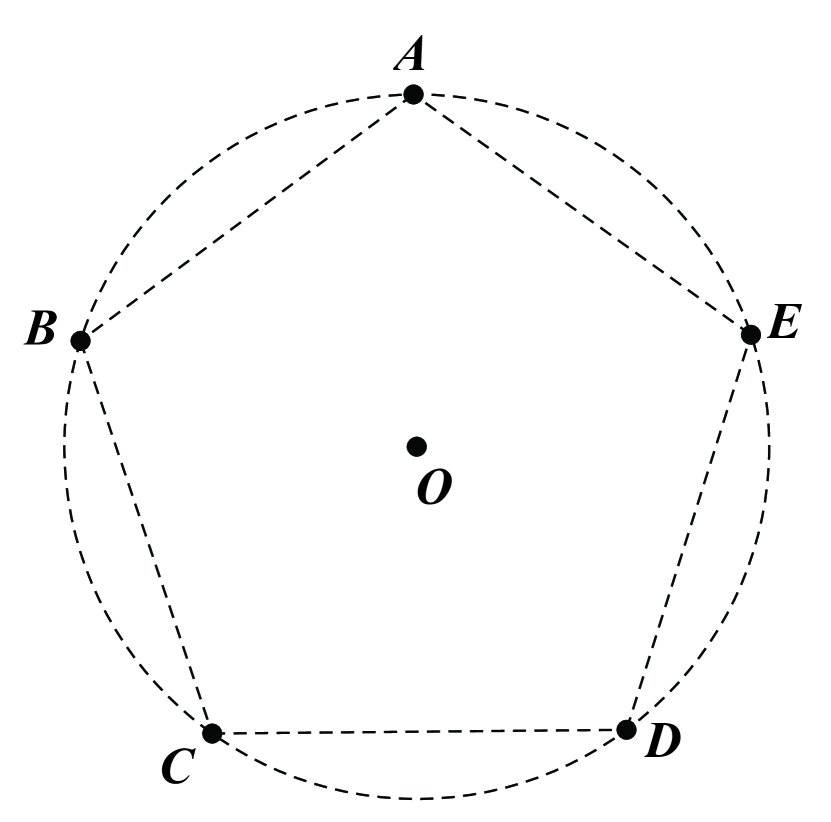
Figure 1: Regular (5+1) model

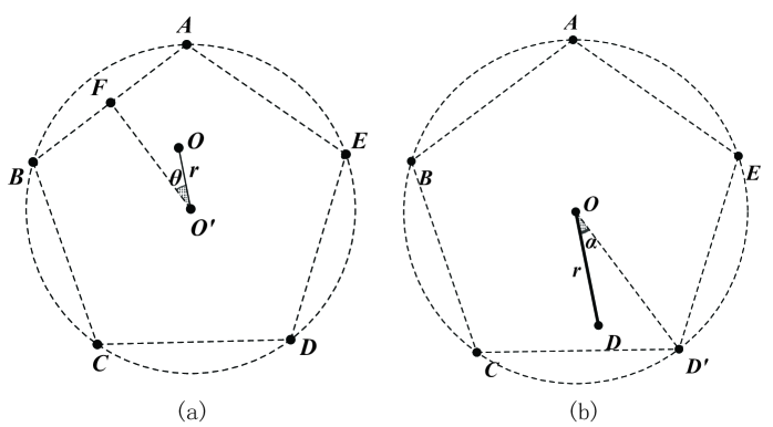
Figure 2: Irregular (5+1) model:
(a) Node Class I; (b) Node Class II

Definition 3

(Irregular (5+1) Model) One of the terminal nodes in the regular (5+1) model deviates from its original position. There are mainly two classifications: Node Class I and Node Class II. The terminal node $O$ denotes the single source terminal node and the terminal nodes $A\sim E$ denote five sink terminal nodes (See Fig.2).

Definition 4

(Node Class I) The terminal node at the circumcenter is allowed to move arbitrarily inside the circle. In this Node Class, the terminal node $O$ is the center terminal node that is allowed to move arbitrarily, while node $O^{\prime}$ is the center of the circumcircle that is fixed. $r$ is depicted as the distance between the center terminal node $O$ and node $O^{\prime}$, and $\theta$ is denoted as $\angle OO^{\prime}F$ where $F$ is the midpoint of the line $AB$ (See Fig.2 (a)).

Definition 5

(Node Class II) One of the five terminal nodes on the circumcircle is allowed to move arbitrarily. In this Node Class, node $D^{\prime}$ is at the place of one sink terminal node in regular model. $r$ is depicted as the distance between the terminal nodes $O$ and $D$, and $\alpha$ is denoted as $\angle DOD^{\prime}$ (See Fig.2 (b)).

III Performance of Network Coding in Space

III-A Cost of Network Coding in space for Node Class I

The construction of network coding in space is depicted in Fig.3 (a), and the hollow nodes are relay nodes.

The shaded region where network coding in space works when $0\leq\theta\leq 36\textordmasculine$ and $r\geq 0$ is shown in Fig.3 (b). Only the case that $\theta$ ranges from 0 to 36º clockwise is necessarily the one to be discussed about because of the symmetry and $\angle AO^{\prime}B$= 72º. $\angle BOA$ should be smaller than 120º according to the Lune property[10], otherwise SIF can not help. As shown in Fig.3 (b), $\angle AOB\geq$120º when the terminal node $O$ moves into arc $\wideparen{AGB}$ where $\angle AGB=120\textordmasculine$.

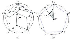
Figure 3: Network coding model for Node Class I:
(a) construction of network coding in space;
(b) region where network coding in space works

Four source flows in space alternately transmit messages $a$ and $b$ while one coding flow transmits the encoded message $a\bigoplus b$, as shown in Fig.3 (a). Consequently, five sink terminal nodes receive two bits of different messages simultaneously, and $f_{e}$ =$\frac{1}{2}$ under the assumption that the maximum flow of each sink is unit. Thus the cost of network coding in space can be calculated as follows:

$L_{NC-I}=\frac{1}{2}\times\sum_{e}(\bigparallel e\bigparallel)=\\ ~{}~{}~{}\frac{1}{2}\times\sqrt{r^{2}-4\sin 66\textordmasculine r\cos\theta+4\sin^{2}66\textordmasculine}\\ +\frac{1}{2}\times\sqrt{r^{2}-4\sin 66\textordmasculine r\cos(\theta+72\textordmasculine)+4\sin^{2}66\textordmasculine}\\ +\frac{1}{2}\times\sqrt{r^{2}-4\sin 66\textordmasculine r\cos(\theta+144\textordmasculine)+4\sin^{2}66\textordmasculine}\\ +\frac{1}{2}\times\sqrt{r^{2}-4\sin 66\textordmasculine r\cos(144\textordmasculine-\theta)+4\sin^{2}66\textordmasculine}\\ +\frac{1}{2}\times\sqrt{r^{2}-4\sin 66\textordmasculine r\cos(72\textordmasculine-\theta)+4\sin^{2}66\textordmasculine}$

III-B Cost of Network Coding in space for Node Class II

The construction of network coding in space is depicted in Fig.4 (a).

The shaded region where network coding in space works when $0\,^{\circ}\leq\alpha\leq 48\,^{\circ}~{}$and $r\geq 0$ is shown in Fig.4 (b). $\angle DOE$, $\angle OCD$ and $\angle CDO$ should be smaller than 120º according to the Lune property [10], otherwise, SIF can not help. From Fig.4 (b), $\angle DOE\geq$120º when the terminal node $D$ moves across the dashed line $OD^{\prime\prime}$ where $\angle D^{\prime\prime}OD^{\prime}=48\textordmasculine$; $\angle OCD\geq 120\textordmasculine$ when the terminal node $D$ moves across the dashed line $CF$ where $\angle OCF=120$º; and $\angle CDO\geq 120\textordmasculine$ when the terminal node $D$ moves inside arc $\wideparen{ORC}$ where $\angle ORC=120$º.

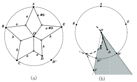
Figure 4: Network coding model for Node Class II:
(a) construction of network coding in space;
(b) region where network coding in space works

The cost of network coding in space can be calculated as follows[9]:
$L_{NC-II}=3\cos{24\,^{\circ}}+$
$\frac{1}{2}\times\sqrt{1+r^{2}-2r\cos{(132\,^{\circ}-\alpha)}}+\frac{1}{2}\times\sqrt{1+r^{2}-\cos{(132\,^{\circ}+\alpha)}}$

IV Performance of Routing in Space

IV-A Cost of Routing in Space for Node Class I

The cost of routing in space for Node Class I can be obtained by the exact algorithms[11] of Euclidean Steiner Minimum Tree (ESMT). The main steps are as follows. First, generate all the constructions of Full Steiner Tree (FST). Second, enumerate all the possible Steiner Trees which are the concatenations of FSTs. Third, calculate the cost of the Steiner Trees and choose the minimum one as ESMT.

IV-A1 Generation of FSTs

Generate all the possible FSTs of the six terminal nodes in the irregular (5+1) model.

IV-A2 Concatenations of FSTs

We mainly consider the concatenation of one FST with three terminal nodes and another FST with four terminal nodes, and the reasons are similar to[8][9]. Moreover, the intersection of FSTs must be the center terminal node $O$ rather than any of the terminal nodes on the circumcircle. All the cases where the intersection of FSTs is the terminal node on the circumcircle can be represented by the three cases shown in Fig.5.

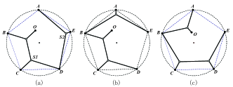
Figure 5: Three cases that should be pruned:
(a) OBCD+DAE; (b) ODCB+BAE; (c) BCDE+ABO

According to [10], if two FSTs share a node $z$, then the two edges meet at $z$ and make at least 120$\textordmasculine$ with each other. However, when two FSTs share the terminal node $D$ (See Fig.5 (a)), $\angle S_{1}DS_{2}<\angle CDE=108\textordmasculine<120\textordmasculine$. Hence, Fig.5 (a) should be pruned. In addition, similar proof can be applied to Fig.5 (b) and Fig.5 (c).

The concatenations of FSTs can be divided into five cases, as shown in Fig.6, Fig.7 and Fig.8. The subcases shown in Fig.7 (b) and Fig.7 (c) are the degenerations of Fig.7 (a), and the subcases shown in Fig.8 (b) and Fig.8 (c) are the degenerations of Fig.8 (a).

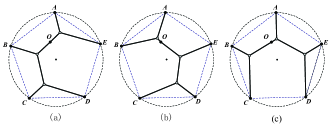
Figure 6: First three cases:
(a) OBCD+OAE; (b) OCDE+OAB; (c) OADE+OBC

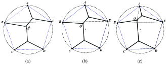
Figure 7: The fourth case OABE+OCD has three subcases:
(a) node O is nondegenerate;
(b) node O degenerates and is below the line BE;
(c) node O degenerates and is above the line BE

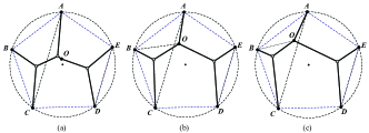
Figure 8: The fifth case OABC+ODE has three subcases:
(a) node O is nondegenerate;
(b) node O degenerates and is on the right of the line AC;
(c) node O degenerates and is on the left of the line AC

In the fourth case, the terminal node $O$ is nondegenerate as shown in Fig.7 (a), when it moves inside the shaded region shown in Fig.10. As shown in Fig.11, $\triangle AFE$ and $\triangle BMO$ are two equilateral triangles constructed to find the FST, and the bold-solid lines construct the FST, in which node $S$ is a Steiner node. We construct the arc $\wideparen{BNF}$ that satisfies $\angle BNF$=120º. As every Steiner node of a Steiner Tree has exactly three lines meeting at 120º[10], node $S$ is on the arc $\wideparen{BNF}$ when the terminal node $O$ moves outside the arc $\wideparen{BNF}$ as shown in Fig.11 (a). However, when the terminal node $O$ moves on the arc $\wideparen{BNF}$ as shown in Fig.11 (b), $\angle BOF$=120º and the terminal node $O$ degenerates into a Steiner node. Furthermore, when the terminal node $O$ moves inside the arc $\wideparen{BNF}$, $\angle BOF$$>$120º, and the terminal node $O$ also degenerates.

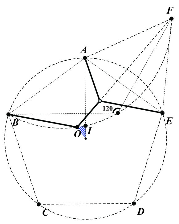
Figure 9: Region that the terminal node O does not degenerate

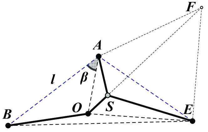
Figure 10: the Steiner node $S$ should lie in $\triangle AOE$

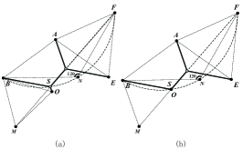
Figure 11: Two cases with supplementary lines:
(a) node $O$ lies outside arc $\wideparen{BNF}$;
(b) node $O$ is on the arc $\wideparen{BNF}$

The terminal node $O$ degenerates as shown in Fig.7 (b), when it moves below the line BE and is outside the shaded region shown in Fig.10. As the terminal node $O$ is below the line BE, terminal nodes $A,~{}B,~{}O,~{}E$ form a convex quadrilateral, and according to[9][10], Fig.7 (b) is obtained.

In addition, the terminal node $O$ degenerates as shown in Fig.7 (c), when it moves above the line BE and is outside the shaded region shown in Fig.10. When the terminal node $O$ is above the line BE and forms a concave quadrilateral $ABOE$, the Steiner node should lie in triangle $\triangle AOE$ rather than in triangle $\triangle AOB$. As shown in Fig.10, $\angle AOE<\angle AOB$. Let $\angle BAO=\beta$, then $\angle EAO=108\textordmasculine-\beta$. Suppose $\angle AOB\leq 120\textordmasculine$, otherwise no Steiner node could possibly exist in $\triangle AOB$[10]. Let $AO=x$, $AB=AE=l$, then $OE=\sqrt{x^{2}+l^{2}-2xl\cos(108\textordmasculine-\beta)}$, $BO=\sqrt{x^{2}+l^{2}-2xl\cos\beta}$.
(1) If the Steiner node $S$ lies inside $\triangle AOE$, ${L_{1}}$ denotes the cost of the FST and it is given by:
${L_{1}}$=$\sqrt{x^{2}+l^{2}-2xl\cos(168\textordmasculine-\beta)}$+$\sqrt{x^{2}+l^{2}-2xl\cos\beta}$,
(2) else if the Steiner node $S$ lies inside $\triangle AOB$, ${L_{2}}$ denotes the cost of the FST and it is given by:
${L_{2}}$=$\sqrt{x^{2}+l^{2}-2xl\cos(\beta+60\textordmasculine)}$+$\sqrt{x^{2}+l^{2}-2xl\cos(108\textordmasculine-\beta)}$.

Let $F(\beta)={L_{1}}-{L_{2}}$ $(0\leq\beta\leq 54\textordmasculine)$. Calculations show that $F^{\prime}(\beta)\geq$0, $F(\beta)_{max}$=$F(54\textordmasculine)$ =0. Hence, ${L_{1}}\leq{L_{2}}$, and the Steiner node should lie in triangle $\triangle AOE$ and Fig.7 (c) is obtained.

The fifth case has three subcases shown in Fig.8, similarly to the fourth case.

IV-A3 Computations of ESMT

Computations of ESMT are divided into five cases, and ESMT is the one that has the minimum cost.

(1) The first case: $OBCD+OAE$ (See Fig.12)

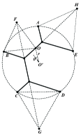
Figure 12: Detailed calculation of the first case OBCD+OAE

$\triangle OBF,~{}\triangle CDG$ and $\triangle AEH$ are three equilateral triangles, and node $O^{\prime}$ is the circumcenter, as shown in Fig.12.

In $\triangle BO^{\prime}O$, $\angle BO^{\prime}O=36\textordmasculine+\theta=\alpha$, $OO^{\prime}=r$ and $O^{\prime}A$=1. According to the law of cosines, $BO^{2}=1+r^{2}-2r\cos\alpha$, $\cos(\angle O^{\prime}BO)=(1-r\cos\alpha)/BO$. In addition, we can obtain $\sin(\angle O^{\prime}BO)=r\sin\alpha/BO$,  $\tan(\angle O^{\prime}BO)=r\sin\alpha/(1-r\cos\alpha)$ by using the law of sines.

In $\triangle BO^{\prime}G$, $\angle BO^{\prime}G=108\textordmasculine$, $O^{\prime}G=2\sin 66\textordmasculine=\beta$ . Similarly we can obtain $\tan(\angle GBO^{\prime})=(\beta\sin 108\textordmasculine)/(1-\beta\cos 108\textordmasculine)$, $\cos(\angle GBO^{\prime})=(1-\beta\cos 108\textordmasculine)/GB$, $\sin(\angle GBO^{\prime})=(\beta\sin 108\textordmasculine)/GB$.

In $\triangle FBG$, $FB^{2}=1+r^{2}-2r\cos\alpha$, $BG^{2}=1+\beta^{2}-2\beta\cos 108\textordmasculine$, $\cos(\angle FBG)=\cos(60\textordmasculine+\angle OBO^{\prime}+\angle O^{\prime}BG)=1/(BK\times GB)[0.5-r\sin(\alpha+30\textordmasculine)-\beta\sin 138\textordmasculine+\beta r\sin(138\textordmasculine+\alpha)]$. By using the law of cosines, $\cos\angle FBG=(FB^{2}+BG^{2}-FG^{2})/(2FB\times BG)$. As a result, $FG^{2}=1+r^{2}+2r\sin(\theta+6\textordmasculine)+4r\sin(\theta-6\textordmasculine)\sin 66\textordmasculine+4(\sin^{2}66\textordmasculine)-4\sin 66\textordmasculine\cos 168\textordmasculine$.

In $\triangle O^{\prime}OH$, $\angle OO^{\prime}H=36\textordmasculine$, $O^{\prime}O=r$, $O^{\prime}H=\beta=2\sin 66\textordmasculine$. According to the law of cosines, $OH^{2}=r^{2}-4r\sin 66\textordmasculine\cos(72\textordmasculine-\theta)+4\sin^{2}66\textordmasculine$.

Hence, ${L_{I-1}}=FG+OH$.
${L_{I-1}}=[r^{2}-4\sin 66\textordmasculine rcos(72\textordmasculine-\theta)+4\sin^{2}66\textordmasculine]^{\frac{1}{2}}+$
$[1+r^{2}+2r\sin(\theta+6\textordmasculine)+4\sin 66\textordmasculine r\sin(\theta-6\textordmasculine)+4\sin^{2}66\textordmasculine-4\sin 66\textordmasculine\cos 168\textordmasculine]^{\frac{1}{2}}$

(2) The second case: $OCDE+OAB$ (See Fig.6 (b))
${L_{I-2}}=[r^{2}-4\sin 66\textordmasculine r\cos\theta+4\sin^{2}66\textordmasculine]^{\frac{1}{2}}+[1+r^{2}-2r\cos(168\textordmasculine-\theta)+4\sin 66\textordmasculine r\sin(66\textordmasculine-\theta)+4\sin^{2}66\textordmasculine-4\sin 66\textordmasculine\cos 168\textordmasculine]^{\frac{1}{2}}$

(3) The third case: $OADE+OBC$ (See Fig.6 (c))
$L_{I-3}=[r^{2}-4\sin 66\textordmasculine r\cos(\theta+72\textordmasculine)+4\sin^{2}66\textordmasculine]^{\frac{1}{2}}+[1+r^{2}-2r\sin(\theta-6\textordmasculine)-4\sin 66\textordmasculine r\sin(\theta+6\textordmasculine)+4\sin^{2}66\textordmasculine-4\sin 66\textordmasculine\cos 168\textordmasculine]^{\frac{1}{2}}$

(4) The fourth case: $OABE+OCD$ (See Fig.7)

When the terminal node $O$ is nondegenerate, then $\angle BOF$$<$120º, i.e. $r\cos(36\textordmasculine-\theta)<\cos 72\textordmasculine$ and $\cos(\angle BOF)=$
$\frac{1+2r^{2}-2r\cos(36\textordmasculine+\theta)+4\sin^{2}66\textordmasculine-4r\sin 66\textordmasculine\cos(72\textordmasculine-\theta)-16\sin^{2}36\textordmasculine\sin^{2}84\textordmasculine}{8\times\sqrt{1+r^{2}-2r\cos(36\textordmasculine+\theta)}\times\sqrt{r^{2}-4r\sin 66\textordmasculine\cos(72\textordmasculine-\theta)+4\sin^{2}66\textordmasculine}}>-\frac{1}{2}$,
$L_{I-4-1}=[1+r^{2}-2r\cos(36\textordmasculine+\theta)]^{\frac{1}{2}}+[r^{2}-4\sin 66\textordmasculine r\cos(72\textordmasculine-\theta)+4\sin^{2}66\textordmasculine]^{\frac{1}{2}}+[r^{2}-4\sin 66\textordmasculine r\cos(\theta+144\textordmasculine)+4\sin^{2}66\textordmasculine]^{\frac{1}{2}}$

When the terminal node $O$ degenerates and is below the line $BE$, then $\angle BOF\geq$120º, i.e. $r\cos(36\textordmasculine-\theta)<\cos 72\textordmasculine$ and $\cos(\angle BOF)=$
$\frac{1+2r^{2}-2r\cos(36\textordmasculine+\theta)+4\sin^{2}66\textordmasculine-4r\sin 66\textordmasculine\cos(72\textordmasculine-\theta)-16\sin^{2}36\textordmasculine\sin^{2}84\textordmasculine}{8\times\sqrt{1+r^{2}-2r\cos(36\textordmasculine+\theta)}\times\sqrt{r^{2}-4r\sin 66\textordmasculine\cos(72\textordmasculine-\theta)+4\sin^{2}66\textordmasculine}}\leq-\frac{1}{2}$,
$L_{I-4-2}=[r^{2}-4\sin 66\textordmasculine r\cos(144\textordmasculine+\theta)+4\sin^{2}66\textordmasculine]^{\frac{1}{2}}+[1+r^{2}-2r\sin(66\textordmasculine+\theta)-4\sin 66\textordmasculine r\sin(102\textordmasculine-\theta)+4\sin^{2}66\textordmasculine-4\sin 66\textordmasculine\cos 168\textordmasculine]^{\frac{1}{2}}$

When the terminal node $O$ degenerates and is above the line $BE$, i.e. $r\cos(36\textordmasculine-\theta)\geq\cos 72\textordmasculine$,
$L_{I-4-3}=[r^{2}-4\sin 66\textordmasculine r\cos(\theta+144\textordmasculine)+4\sin^{2}66\textordmasculine]^{\frac{1}{2}}+[1+r^{2}-2r\sin(66\textordmasculine+\theta)-4\sin 66\textordmasculine r\sin(102\textordmasculine-\theta)+4\sin 66\textordmasculine\cos 168\textordmasculine]^{\frac{1}{2}}$

(5) The fifth case: $OABC+ODE$ (See Fig.8)

When the terminal node $O$ is nondegenerate:
$L_{I-5-1}=[1+r^{2}-2r\cos(36\textordmasculine-\theta)]^{\frac{1}{2}}+[r^{2}-4\sin 66\textordmasculine r\cos(\theta+72\textordmasculine)+4\sin^{2}66\textordmasculine]^{\frac{1}{2}}+[r^{2}-4\sin 66\textordmasculine r\cos(144\textordmasculine-\theta)+4\sin^{2}66\textordmasculine]^{\frac{1}{2}}$

When the terminal node $O$ degenerates and is on the right of the line $AC$:
$L_{I-5-2}=[1+r^{2}-2r\cos(36\textordmasculine-\theta)]^{\frac{1}{2}}+[r^{2}-4\sin 66\textordmasculine r\cos(\theta+72\textordmasculine)+4\sin^{2}66\textordmasculine]^{\frac{1}{2}}+[r^{2}-4\sin 66\textordmasculine r\cos(144\textordmasculine-\theta)+4\sin^{2}66\textordmasculine]^{\frac{1}{2}}$

When the terminal node $O$ degenerates and is on the left of the line $AC$:
$L_{I-5-3}=[r^{2}-4\sin 66\textordmasculine r\cos(144\textordmasculine-\theta)+4\sin^{2}66\textordmasculine]^{\frac{1}{2}}+[1+r^{2}-2r\sin(66\textordmasculine-\theta)-4\sin 66\textordmasculine r\sin(102\textordmasculine+\theta)+4\sin^{2}66\textordmasculine-4\sin 66\textordmasculine\cos 168\textordmasculine]^{\frac{1}{2}}$

IV-B Cost of Routing in Space for Node Class II

Methods are similar with Section IV-$A$. Details refer to [9].

V Numerical Analysis and Results

V-A Node Class I

The functional relation of CA and ($x,y$) in three-dimensional is shown in Fig.13 (a), where only CA$\geq$1 is figured out and cartesian coordinates ($x,y$) are obtained from polar coordinates ($r,~{}\theta$). Furthermore, Fig.13 (a) shows that CA achieves its maximum value of 1.0158 when $r=0$.

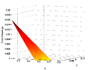
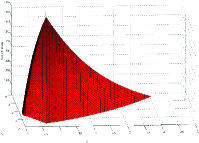
Figure 13: Cost advantage $\geq$1 (3-D):
(a) Node Class I; (b) Node Class II

The two-dimensional region where $CA\geq$1 is shown in Fig.14 (a), and it is obtained by projecting Fig.13 (a) to $XY$ plane. When projected to $XY$ plane, Fig.13 (a) turns out to be a sector whose angle is 36º and its radius is between 0.20 and 0.24. Taking the symmetry of the Node Class I model into consideration, the final projection in two-dimensional is shown in Fig.14 (a). The performance of network coding in space is superior to routing in space in the shaded region, and the maximum value of CA is achieved when the terminal node $O$ is at the center of the circumcircle (i.e. $r=0$).

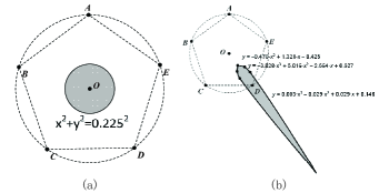
Figure 14: Region where cost advantage $\geq$1 (2-D):
(a) Node Class I; (b) Node Class II

Furthermore, it can be proved that the region where network coding in space outperforms routing in space is a circle, and the maximum value of CA can be achieved when the terminal node $O$ is at the centre of the circumcircle. First, transform the problem of CA$\geq$1 to the problem of $L_{NC-I}\leq min\{L_{I-i}\}~{}(i=1,2,...,5)$, and make sure there is no discontinuity point in the region where CA$\geq$1. Here $L_{I-4}$ and $L_{I-5}$ represents the minimum value of $L_{I-4-j}~{}(j=1,2,3)$, and $L_{I-5}$ represents the minimum value of $L_{I-5-k}~{}(k=1,2,3)$. Second, when $\theta$ is fixed, study the monotonicity of function $f(r,\theta)=L_{NC-I}-min\{L_{I-i}\}$ in order to confirm that the region where CA$\geq$1 is not an annulus or something similar. Third, when $r$ is fixed, study the monotonicity of function $f(r,\theta)=L_{NC-I}-min\{L_{I-i}\}$ in order to confirm that the region where CA$\geq$1 is a circle.

ESMT should be one of the five cases. Furthermore, the problem of obtaining the region where CA$\geq$1 is equivalent to the the problem of obtaining the region where $L_{NC-I}\leq min\{L_{I-i}\}$. $L_{NC-I}$ and $L_{I-1}$ to $L_{I-5}$ are all continuous functions, because they are the linear combinations of some basic functions. As a result, function $Y_{i}=L_{I-i}-L_{NC-I}$ (i=1,2,…,5)  is also a continuous function. In addition, $f(r,\theta)\geq$0 is a three-dimensional curved surface and as a result its projection on the $XY$ Plane is continuous, which means that there exists no discontinuity point in the region where CA$\geq$1.

From equations $L_{I-1}~{}to~{}L_{I-5}$, we can calculate it as follows:

$\frac{d(L_{NC-I})}{dr}=\frac{0.25}{\sqrt{r^{2}-4r\sin 66\textordmasculine\cos\theta+4\sin^{2}66\textordmasculine}}+\frac{0.25}{\sqrt{r^{2}-4r\sin 66\textordmasculine\cos(\theta+72\textordmasculine)+4\sin^{2}66\textordmasculine}}+\frac{0.25}{\sqrt{r^{2}-4r\sin 66\textordmasculine\cos(\theta+144\textordmasculine+4\sin^{2}66\textordmasculine)}}+\frac{0.25}{\sqrt{r^{2}-4r\sin 66\textordmasculine\cos(144\textordmasculine-\theta)+4\sin^{2}66\textordmasculine}}+\frac{0.25}{r^{2}-4r\sin 66\textordmasculine\cos(72\textordmasculine-\theta)+4\sin^{2}66\textordmasculine}$ ,

$\frac{d(L_{I-1})}{dr}=\frac{r+\sin(\theta+6\textordmasculine)+4\sin 66\textordmasculine\sin(\theta-6\textordmasculine)}{\sqrt{1+r^{2}+2r\sin(\theta+6\textordmasculine)+4\sin 66\textordmasculine r\sin(\theta-6\textordmasculine)+4\sin^{2}66\textordmasculine-4\sin 66\textordmasculine\cos 168\textordmasculine}}\\ +\frac{r-2\sin 66\textordmasculine\cos(72\textordmasculine-\theta)}{\sqrt{r^{2}-4\sin 66\textordmasculine r\cos(72\textordmasculine-\theta)+4\sin^{2}66\textordmasculine}}$

Let $y_{1}=\frac{d(L_{NC-I})}{dr}-\frac{d(L_{I-1})}{dr}$, when $\theta=\theta_{0}~{}(\theta_{0}\in[0,36\textordmasculine])$, $r\in$[0,0.24]. $r$ is restricted to [0,0.24] according to the projection of Fig.13 (a). By matlab, we find that $\forall r\in[0,0.24]$, $y_{1}\geq$0. Similar results can be obtained when we calculate the other four functions $y_{2}=\frac{d(L_{NC-I})}{dr}-\frac{d(L_{I-2})}{dr}$ to $y_{5}=\frac{d(L_{NC-I})}{dr}-\frac{d(L_{I-5})}{dr}$, which means that $Y_{i}=L_{NC-I}-L_{I-i}$ (i=1,2,…,5) are all monotonous increasing. As mentioned above, the function $f(r,\theta)=L_{NC-I}-min\{L_{I-i}\}$ is continuous, thus the function $f(r,\theta_{0})=L_{NC-I}-min\{L_{I-i}\}$ is also monotonous increasing when $\theta$ is fixed. The significance of this result is that if $\exists~{}r_{0}$, when $r=r_{0}$, $f(r_{0},\theta_{0})=L_{NC-I}-min\{L_{I-i}\}$=0, then $r_{0}$ is the only parameter that can satisfy the equation $L_{NC-I}=min\{L_{I-i}\}$. In other words, the region where CA$\geq$1 is not an annulus. In addition, we find that when $r$=0, $CA$=1.0158.

Let $f(r_{0},\theta)=L_{NC-I}-min\{L_{I-i}\}$ (i=1,2,…,5), when $r=r_{0}~{}(r_{0}\in[0.20,0.24])$, $\theta\in[0,36\textordmasculine]$. Calculations show that when $r~{}(0.20\leq r\leq 0.24)$ is fixed, $\frac{df(r_{0},\theta)}{d\theta}\geq$0, which means that if $\exists~{}r_{1}\in[0.20,0.24],~{}f(r_{1},0)=0$ and $f(r_{1},36\textordmasculine)$=0, then $f(r_{1},\theta)$=0 satisfies all of the possibilities when $\theta$ ranges from 0 to 36º, which means the region that satisfies $CA\geq$1 is a circle. Furthermore, $r_{1}$ indeed exists and $r_{1}$=0.225 by matlab.

V-B Node Class II

The functional relation of CA and ($x,y$) for Node Class II in three-dimensional is shown in Fig.13 (b), where only CA$\geq$1 is depicted, and cartesian coordinates ($x,y$) are obtained from polar coordinates ($r,~{}\alpha$). Furthermore, Fig.13 (b) shows that CA achieves its maximum value of 1.0158 when ($r,\alpha$)=(1,0). The coordinates of node $D^{\prime}$ in the irregular (5+1) model is ($r,\alpha$)=(1,0). From Fig.13 (b), the closer the terminal node $D$ moves to the node $D^{\prime}$, the greater the value of CA gets. CA achieves its maximum value when the terminal node $D$ coincides with the node $D^{\prime}$.

The two-dimensional region where CA$\geq$1 for Node Class II is shown in Fig.14 (b).

VI Properties and Discussion

Different from that of routing in space, some properties of SIF can be described as follows: (1) Either the center terminal node or one terminal node on the circumcircle moves arbitrarily, the maximum value of CA is achieved when the irregular (5+1) model turns back to the regular (5+1) model.  (2) The number of relay nodes can be greater than $n-2$ in SIF while this number can not be greater than $n-2$ in ESMT.  (3) A given terminal node can have a degree which can be greater than three while the degree can not be greater than three in ESMT.

Furthermore, the center terminal node $O$ (for Node Class I) can only move in the dashed circle shown in Fig.15, whose diameter is around 0.450. The minimum distance between one terminal node on the circumcircle and the center terminal node $O$ is around 0.450 (i.e. if the terminal node $D$ for Node Class II moves inside the solid-line circle shown in Fig.15, CA will be less than one), which is nearly equal to the diameter mentioned above. Thus, we conjecture Position Independence Property. From Fig.15, whatever the position of any terminal node outside the solid circle, or if any terminal node does move anywhere outside the solid circle, the distance between the moving node and the center terminal node $O$ will always be greater than the minimum distance of 0.450 required to achieve CA$\geq$1. The maximum moving distance of the center terminal node is equivalent to the minimum distance between the center terminal node and any other terminal nodes on the circumcircle. Thus, the position of the terminal node does not influence the performance of SIF. In addition, any two terminal nodes can not move too close to each other, otherwise SIF can not help. For example, if the terminal node $O$ moves outside the dashed circle and gets too close to the terminal nodes $A$ and $B$, then it will be too far from the terminal nodes $C$, $D$ and $E$, which will make routing in space superior to network coding in space, meaning that SIF can not help.

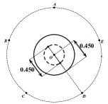
Figure 15: Position Independence

There are following interesting questions to answer: When any two terminal nodes are allowed to move arbitrarily, does CA achieve its maximum value only when the irregular (5+1) model turns back to the regular (5+1) model? When any three terminal nodes are allowed to move arbitrarily, does CA achieve its maximum value only when the irregular (5+1) model turns back to the regular (5+1) model? What if any four terminal nodes are allowed to move arbitrarily? What if any five terminal nodes in this regular (5+1) model are allowed to move arbitrarily, which is equivalent to all the terminal nodes are allowed to move arbitrarily? Furthermore, if given six terminal nodes whose positions are arbitrary, when and how is SIF superior to routing in space? In other words, when given n terminal nodes in space arbitrarily, does SIF help when n=6? Does CA achieve its maximum value only when the six terminal nodes form the regular (5+1) model? It is known that Yin $et~{}al$[4] proposed questions whether SIF can help when n=4 or n=5. Furthermore, Yin has already proved that SIF does not help when n=3.

VII Conclusions

This work compares the performance between network coding in space and routing in space based on two classes of irregular (5+1) model, which are Node Class I and Node Class II. Furthermore, CA in both irregular models achieves its maximum value of 1.0158 only when the irregular (5+1) model turns back into regular (5+1) model. The ongoing work is to answer above questions in order to study SIF properties.

References

- [1] R. Ahlswede, N. Cai, S.Y.R. Li, and R.W. Yeung. Network information Flow. IEEE Trans. on Information Theory, 46(4):1204-1216, 2000.
- [2] Z. Li, B. Li, and L. C. Lau. On achieving maximum multicast throughput in undirected networks. IEEE Trans. on Information Theory, 52(6):2467-2485, 2006.
- [3] S. Maheshwar, Z. Li, and B. Li. Bounding the coding advantage of combination network coding in undirected networks. IEEE Trans. on Information Theory, 58(2):570-584, 2012.
- [4] X. Yin, Y. Wang, X. Wang, X. Xue, Z. Li, Min-Cost Multicast Networks in Euclidean Space. IEEE International Symposium on Information Theory (ISIT), 2012.
- [5] T. Xiahou, C. Wu, J. Huang, Z. Li, A Geometric Framework for Investigating the Multiple Unicast Network Coding Conjecture. Netcod, 2012.
- [6] J. Huang, X. Yin, X. Zhang, X. Du and Z. Li, On Space Information Flow: Single Multicast. Netcod, 2013.
- [7] J. Huang, F. Yang, K. Jin, Z. Li, Network Coding in Two-dimension Euclidean Space. Journal of Chongqing University of Posts and Telecommunications (Natural Science Edition) Oct. 2012.
- [8] X. Zhang and J. Huang, Superiority of Network Coding in Space for Irregular Polygons. IEEE 14th International Conference on Communication Technology (ICCT), 2012.
- [9] T. Wen, X. Zhang, X. Huang, J. Huang, Cost Advantage of Network Coding in Space for Irregular 5+1 Model. IEEE 11th International Conference on Dependable, Autonomic and Secure Computing (ICDASC), 2013.
- [10] E.N. Gilbert and H.O. Pollak. Steiner Minimal Trees. SIAM Journal on Applied Mathematics, 16(1): 1-29, 1968
- [11] P. Winter and M. Zachariasen, Exact Algorithms for Plane Steiner Tree Problems: A Computational Study. Combinatorial Optimization Volume 6, 2000, pp 81-116.